the Creative Commons Attribution 4.0 License.
the Creative Commons Attribution 4.0 License.
 | 01 Sep 2021
The Antarctic Coastal Current in the Bellingshausen Sea
Andrew F. Thompson
Kevin Speer
Lena Schulze Chretien
Yana Bebieva
The ice shelves of the West Antarctic Ice Sheet experience basal melting induced by underlying warm, salty Circumpolar Deep Water. Basal meltwater, along with runoff from ice sheets, supplies fresh buoyant water to a circulation feature near the coast, the Antarctic Coastal Current (AACC). The formation, structure, and coherence of the AACC has been well documented along the West Antarctic Peninsula (WAP). Observations from instrumented seals collected in the Bellingshausen Sea offer extensive hydrographic coverage throughout the year, providing evidence of the continuation of the westward flowing AACC from the WAP towards the Amundsen Sea. The observations reported here demonstrate that the coastal boundary current enters the eastern Bellingshausen Sea from the WAP and flows westward along the face of multiple ice shelves, including the westernmost Abbot Ice Shelf. The presence of the AACC in the western Bellingshausen Sea has implications for the export of water properties into the eastern Amundsen Sea, which we suggest may occur through multiple pathways, either along the coast or along the continental shelf break. The temperature, salinity, and density structure of the current indicates an increase in baroclinic transport as the AACC flows from the east to the west, and as it entrains meltwater from the ice shelves in the Bellingshausen Sea. The AACC acts as a mechanism to transport meltwater out of the Bellingshausen Sea and into the Amundsen and Ross seas, with the potential to impact, respectively, basal melt rates and bottom water formation in these regions.
- Article
(11252 KB) - Full-text XML
- BibTeX
- EndNote


The Antarctic continental slope in West Antarctica, spanning the West Antarctic Peninsula (WAP) to the western Amundsen Sea, is characterized by a shoaling of the subsurface temperature maximum, which allows warm, salty Circumpolar Deep Water (CDW) greater access to the continental shelf. This leads to an increase in the oceanic heat content over the shelf in this region compared to other Antarctic shelf seas (Schmidtko et al., 2014). Some of the largest basal melt rates experienced by Antarctic ice shelves occur in the Amundsen and Bellingshausen seas due to the flow of warm CDW towards the coast and into ice shelf cavities (The IMBIE team, 2018; Paolo et al., 2015; Pritchard et al., 2012). Over most of the satellite record, there is evidence for increased basal melting throughout West Antarctica (e.g., Jenkins et al., 2018), although there is also evidence for significant interannual variability (Holland et al., 2019) and a reduction in melt rates in recent years (Paolo et al., 2018; Adusumilli et al., 2020).
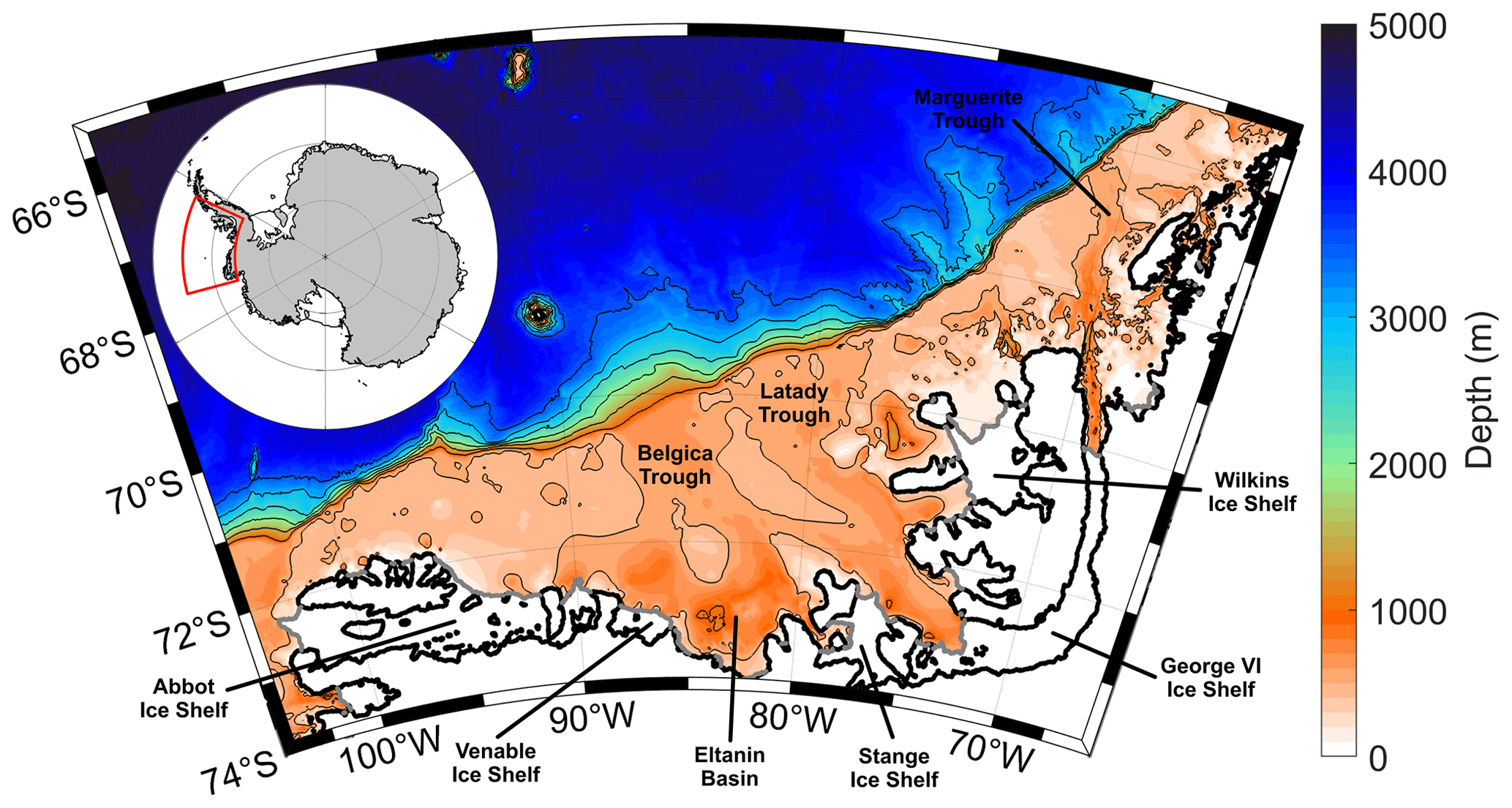
Figure 1Bathymetry of the Bellingshausen Sea and West Antarctic Peninsula continental shelves (red box in the inset plot) as given by the RTopo2 data product (Schaffer et al., 2016). Thin black contours delineate isobaths between 0 and 3000 m, with a 500 m interval. Thick black and gray lines indicate the coastline and the edge of permanent ice shelves, respectively. Key geographic features are labeled.
The delivery of warm CDW to the base of Antarctica's floating ice shelves depends on an intricate continental shelf circulation that, under the influence of topography, is largely organized into frontal currents. Significant attention has been devoted to understanding how the frontal structure at the Antarctic shelf break and its associated westward flow, referred to as the Antarctic Slope Front (ASF) and the Antarctic Slope Current (ASC), respectively, enables heat transport onto the continental shelf (Whitworth et al., 1998; Thompson et al., 2018). Over the continental shelf itself, a major circulation feature is the Antarctic Coastal Current (AACC), which also flows westward along the coast of the Antarctic continent. While the ASF is typically defined by a strong gradient in temperature, marked by the southernmost extent of unmodified CDW (Whitworth et al., 1998), the AACC is typically characterized by a strong gradient in salinity. The first observations of the AACC were recorded by Sverdrup (1953) in the Weddell Sea in which he noted that a westward-flowing current split around 0∘, with one branch continuing along the coastline into the Weddell Sea.
Throughout this study, the AACC will be defined as the current bounded on the shoreward side by either the coastline or the face of ice shelves. Similar to the ASC, the AACC may arise in response to both surface mechanical and buoyancy forcing, and the relative importance of these two may impact the current's vertical structure. The AACC in the Weddell Sea is characterized as being primarily a barotropic current, where wind is the main factor in its barotropic variability (Núñez-Riboni and Fahrbach, 2009). Closer to the Weddell–Scotia Confluence, Heywood et al. (2004) described the AACC as a fast and shallow flow in the continental shelf region. Moffat et al. (2008) describe the coastal flow on the WAP as being a baroclinic current driven by strong density gradients, generated by buoyancy input from meltwater and runoff, although they also acknowledged the importance of wind forcing. A coastal current is also found along the WAP in wind-forced numerical simulations controlled by the prevailing easterly winds (Holland et al., 2010), despite the absence of runoff and weak meltwater forcing. Thus, the flow of the AACC throughout West Antarctica and its variability is linked to both wind and buoyancy forcing (Moffat et al., 2008; Holland et al., 2010; Kim et al., 2016; Kimura et al., 2017).
Focusing specifically on West Antarctica, the AACC shows regional differences in its formation and maintenance. Smith et al. (1999) described the AACC as a result of northeasterly winds piling water along the coast. The current then becomes more strongly baroclinic as meltwater is introduced near Marguerite Trough (Smith et al., 1999). This study also suggested that the current could continue into the Bellingshausen Sea, but there was insufficient data to support this suggestion. Moffat et al. (2008) emphasized seasonal variations in the coastal current, which they referred to as the Antarctic Peninsula Coastal Current. We will show below that this circulation feature extends well beyond the Antarctic Peninsula; hence, we will refer to this extensive coastal current system as the Antarctic Coastal Current (AACC). Moffat et al. (2008) argued that the AACC forms during the spring and summer ice-free season, and that it disappears during the winter when sea ice formation and a reduction in meltwater fluxes reduces lateral density gradients. The AACC has been studied in the Bellingshausen Sea using coupled models and connecting the current in the WAP to the Amundsen Sea (Assmann et al., 2005; Holland et al., 2010). Assmann et al. (2005) used a coupled ice–ocean model to reveal a westward flow of sea ice along the coastline that is part of a large cyclonic circulation that flows from the WAP, through the Bellingshausen Sea into the Amundsen and Ross seas. Sea ice drift in this model primarily occurs due to wind forcing, but surface ocean currents also push the sea ice to the west. Holland et al. (2010), through the use of a wind forced ice–ocean–atmosphere model, revealed that in summer and autumn a coastal current starts in the WAP and flows southwestward into the Bellingshausen Sea and exits as a strong westward flow to the north of the Abbot and Venable ice shelves. The authors speculated that this coastal current is a continuation of the current found in Moffat et al. (2008), and that it most likely continues into the Amundsen Sea (Holland et al., 2010).
Direct ship-based measurements of the AACC over the continental shelf in the Bellingshausen Sea region (Fig. 1) are limited. Jenkins and Jacobs (2008) studied the flow under the George VI Ice Shelf, noting that warm CDW floods the continental shelf, causing melting beneath the ice shelf, which escapes to the south. There is a cyclonic circulation in each of the major troughs in the Bellingshausen Sea, where warm CDW flows shoreward along the eastern boundary of the troughs up to the ice shelves (Schulze Chretien et al., 2021). Subsequent ice shelf melt introduces freshwater, creating modified CDW that then flows away from the shore along the western boundary of the troughs (Zhang et al., 2016; Thompson et al., 2020; Schulze Chretien et al., 2021). However, there have been no direct observations of the AACC in the Bellingshausen Sea. In the western Amundsen Sea, the AACC has been identified as being a strong westward current generated by easterly winds, with a variable baroclinic component (Kim et al., 2016). Kimura et al. (2017) explain that a high volume of meltwater is introduced from the ice shelves in the region, establishing a strong baroclinic flow to the west. This flow then exits along the northwestern side of the Amundsen Sea and flows towards the Ross Sea (Assmann et al., 2005; Kim et al., 2016; Kimura et al., 2017; Nakayama et al., 2020). Through the connection between the WAP and the Amundsen Sea, the presence of the AACC in the Bellingshausen Sea has been implied, but not demonstrated, using direct observations.
The AACC provides an important transport pathway that connects various regional seas throughout West Antarctica and potentially even further to the west (Nakayama et al., 2020). The AACC may also play a key role in the overturning circulation over the continental shelf by modifying the vertical stratification. Silvano et al. (2018) showed that freshwater fluxes into the surface ocean stratify the upper ocean, reducing heat loss to the atmosphere and enhancing the transfer of heat to the base of ice shelves. Similar stratification responses and a warming of shelf waters have been highlighted in recent numerical studies (Bronselaer et al., 2018; Golledge et al., 2019; Moorman et al., 2020), although the full potential for feedbacks has not been explored due to either the coarse resolution of these simulations or their lack of ice shelf cavities. Flowing along the face of the major ice shelves in West Antarctica, the AACC has an important role for establishing the partitioning of vertical and lateral heat transport and provides a key link between regional forcing and remote responses.
The purpose of this study is to investigate the horizontal and vertical distribution of temperature, salinity, and density over the continental shelf of the Bellingshausen Sea with a view to mapping the structure and evolution of the AACC. Here we used hydrographic observations obtained from instrumented elephant seals, i.e., a data set that enables the generation of gridded, horizontal maps of hydrographic properties. The frontal structure of the AACC is explored by creating composite hydrographic sections from the seal data. The strength and spatial evolution of the AACC will be considered by diagnosing dynamic height, geostrophic velocities, and volume transports.
Data collected from instrumented southern elephant seals provide the basis for this investigation of the physical properties and circulation on the shelf in the Bellingshausen Sea (Roquet et al., 2017). This study makes use of nearly 20 000 seal profiles from the Bellingshausen Sea that were originally analyzed by Zhang et al. (2016) and an additional 10 000 profiles that extend further to the northeast over the WAP. Figure 2 shows the spatial extent of the available seal data in the Bellingshausen Sea region. The seal data span the years 2007 to 2014, although there is a gap in observations between 2010 and 2013. Just over 22 000, or 73 % of the profiles were collected during “winter” months (April–September), as compared to “summer” months (October–March), thus predominantly showing properties when sea ice covers most of the shelf. Critically, this a period when ship-based observations in the region are almost completely unavailable.
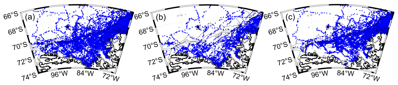
Figure 2Distribution of (a) all seal data, (b) seal data in summer months (October–March), and (c) seal data in winter months (April–September) from the Marine Mammals Exploring the Oceans Pole to Pole (MEOP-CTD) database within the Bellingshausen Sea. Contours are the same as in Fig. 1.
2.1 Southern elephant seal data
In this study, hydrographic data from instrumented elephant seals are analyzed, a subset of which was previously analyzed by Zhang et al. (2016, Fig. A1). We accessed data from the Marine Mammals Exploring the Oceans Pole to Pole (MEOP-CTD; Conductivity–Temperature–Depth) database where CTD–Satellite Relay Data Loggers (CTD–SRDL) are deployed on elephant seals (Roquet et al., 2013). A total of 29 967 hydrographic profiles were analyzed in the Bellingshausen Sea and the WAP. This represents an increase over the 19 893 profiles analyzed by Zhang et al. (2016) due to the additional data along the WAP. These data cover periods from 2005 to May 2006, 2007 to 2010, the austral summer of 2013 and 2014, and June 2015, giving it broad coverage both spatially and temporally. The majority of the seal dives were collected during austral autumn and winter. Figure 2b and c show the seasonal differences in seal sampling in the Bellingshausen Sea. During summer (Fig. 2b), the seal profiles tend to be focused near the coast and over the continental shelf, whereas during winter (Fig. 2c), the seal profiles are more concentrated in the northeastern part of the shelf and along the shelf break. This is an important distinction due to the potential for seasonality in the AACC, although we note that near-coastal observations are not completely absent in winter months. Throughout this study, we report the median properties of the AACC using all available data. Data were produced for both mean and median quantities, but there were not significant differences between the two quantities.
For each profile, we follow the method described in Zhang et al. (2016) where properties are linearly interpolated onto a vertical, nonuniform grid with 52 depth bins. All data have undergone temperature and salinity calibration. Following the MEOP standard, calibration was conducted based on historical data in nearby regions (Roquet et al., 2011). The calibrated data have estimated uncertainties of ±0.02 ∘C for temperature and a ±0.02 practical salinity unit (psu) for salinity. Additional information about data calibration can be found in Zhang et al. (2016).
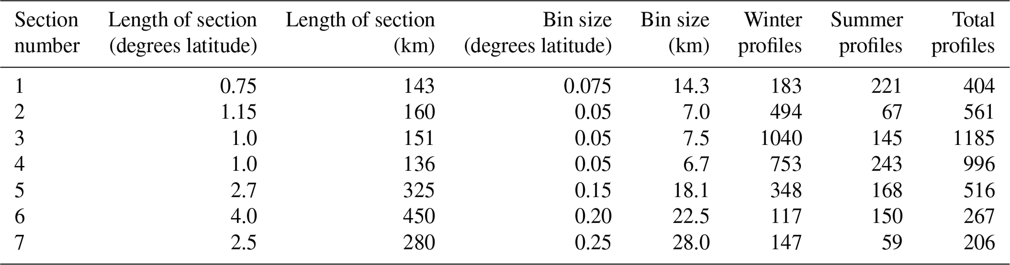
Table 1Length of section (degrees latitude; kilometers), number of winter (April–September), summer (October–March), total profiles, and the averaging length (degrees latitude; kilometers) for each of the seven hydrographic sections shown in Fig. 3.
2.2 Horizontal maps
To assess the horizontal variability in the physical properties in the Bellingshausen Sea shelf region, the seal data were mapped onto a 1∘ longitude by 0.5∘ latitude grid (Fig. 4a). This grid size was chosen to provide the highest resolution on the shelf, while maintaining an adequate number of grid cells that contain at least one data point. We note that if the AACC is narrower than our grid, then the front would look broader than it actually is; in some regions, the AACC has been observed to be a narrow feature of roughly 20 km (Moffat et al., 2008). However, the horizontal maps, and the subsequent dynamic height plot, are important for documenting the structure and extent of the AACC. In each grid cell, and for each depth bin, the median values of temperature and salinity were calculated from the seal dives in that cell, as well as the variance. Separate calculations for summer and winter months were also completed. The dynamic height, referenced to 400 m, was calculated from the median values.
2.3 Hydrographic sections
A total of seven composite hydrographic sections, spanning the continental shelf break to the coast, were created to examine how the vertical structure of physical properties in the Bellingshausen Sea changes from east to west. All of the sections, with the exception of section 1, have more winter profiles than summer profiles, which biases the properties on the shelf in each section towards winter values. Of the sections, two are located in the WAP to compare the seal data with the AACC observations reported in Moffat et al. (2008). The other five sections are located in the Bellingshausen Sea (Fig. 3). A moving median of the seal profiles was taken using a different length scale for each section, based on the available data. For example, in section 1, the length of the section is 0.75∘ of latitude and the medians of the properties were taken every 0.075∘ of latitude. The length scale over which the median was calculated was similar across various sections but was allowed to vary to ensure that each section avoided gaps with unavailable data. A varying bin width did not qualitatively or quantitatively change our results. We chose to use degrees of latitude for convenience because the distance in kilometers is slightly different in each section. Table 1 provides details about the number of profiles, length, and averaging length for each of the seven sections.
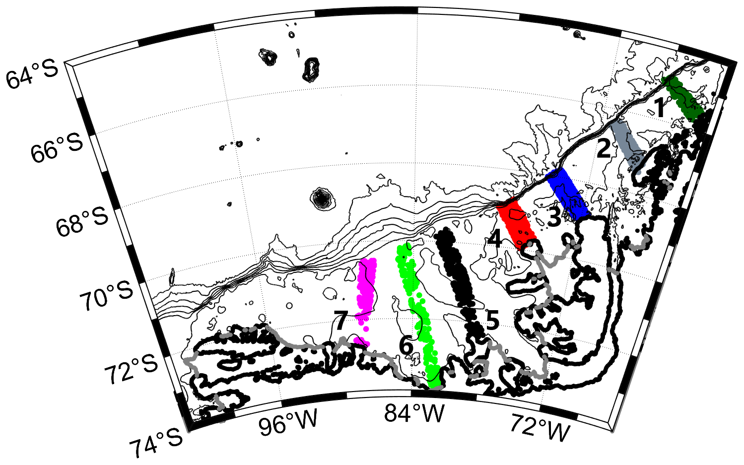
Figure 3Distribution of profiles from instrumented seals used to construct composite, cross-shelf hydrographic sections. The transects are numbered consecutively from 1, at the most northeastern end over the West Antarctic Peninsula shelf (see Appendix; Fig. A1), to 7, at the western edge of the Bellingshausen Sea. Contours are the same as in Fig. 1.
To characterize the strength of the AACC, geostrophic velocities and transports perpendicular to each section were calculated based on the density structure. In order to calculate the total geostrophic velocity and transport, a reference level, or level of no motion, must be selected. A reference level of 400 m was applied to ensure that the full depth of the AACC was captured. This depth roughly marks the lower boundary of the water column exhibiting significant freshwater anomalies that we attribute to meltwater. Some sections reveal a slight flow reversal below our reference level; however, the bulk of the baroclinic coastal current is above this reference level. We have opted to keep the level of no motion consistent across all composite hydrographic sections to limit the impact of varying topography. In Sect. 4, we also present the geostrophic transport referenced to 200 m for comparison with the velocity structure in Moffat et al. (2008), who found a zero crossing for velocity based on shipboard acoustic Doppler current profiler (ADCP) data close to 200 m. Regardless of the reference level applied, the volume transport of the AACC was defined as the vertical integral of the referenced geostrophic velocities between the sea surface and the depth of the 34.4 psu isohaline, as in Moffat et al. (2008). In order to define the offshore extent of the AACC for each section, we first found the center of the AACC by calculating where the gradient in net transport was greatest. We then searched in the offshore direction for the location where the depth-integrated velocity was 15 % of the value at the center of the AACC. We chose to use 15 % of the maximum value because it returned locations that corresponded with a leveling off of the net transport for each section.
To provide an estimate of the error in the velocity/transport calculations, we applied a bootstrapping approach (Efron and Tibshirani, 1994). Along each section, 1000 different composite hydrographic sections were created by randomly selecting only 40 % of the profiles in each cross-shelf bin. Geostrophic velocities and geostrophic transports were calculated for each of these 1000 sections, and error bars are reported as the root mean square (RMS) of these values. The RMS values are taken as the difference from the mean composite section using all the data.
Water properties in the Bellingshausen Sea can be broadly categorized in terms of the following four main water masses: Antarctic Surface Water (AASW), CDW, winter water (WW), and meltwater. The temperature of AASW is directly influenced by surface heat fluxes, but the salinity of AASW can be modified by a broad range of processes, including precipitation/evaporation, runoff from land, sea ice formation and melt, and glacial meltwater (Meredith et al., 2013; van Wessem et al., 2017). Only the latter has a subsurface expression when it is sourced from the base of floating ice shelves, and it appears as a mixture of pure meltwater with other properties, giving rise to a glacially modified version of CDW and/or WW (Fig. 5) (Castro-Morales et al., 2013; Schulze Chretien et al., 2021). Each of these freshwater sources have distinct isotopic signatures (Meredith et al., 2008) but are difficult to distinguish with the tracers provided by the instrumented seals. Due to these limitations, we do not explicitly discuss the distribution of meltwater fractions in this study. Recent studies of the meltwater distribution in the Bellingshausen Sea can be found in Schulze Chretien et al. (2021) and Ruan et al. (2021).
AASW, which represents the surface mixed layer, has potential temperatures ranging from −1.8 to 1 ∘C and salinity ranges from 33 to 34 psu. During austral winter, surface heat loss leads to a deeper mixed layer. In summer, surface heating and freshening from sea ice melt restratifies the surface ocean and leads to shallower mixed layers (Jenkins and Jacobs, 2008; Whitworth et al., 1998). Remnant properties of the wintertime deep mixed layer comprise the WW water mass that is expressed as a temperature minimum layer from −1.8 to −1.5 ∘C and a salinity of about 34.1 psu. WW typically ranges from σ0=27.2 to 27.4 kg m−3, where σ0 is potential density referenced to the surface. Below the pycnocline lies CDW, which is relatively warm and salty, with values from 1 to 1.5 ∘C and 34.7 and 34.85 psu, respectively. CDW occupies the water column from the seafloor to the base of the pycnocline. Since CDW occupies a large portion of the water column, it is an important source of heat over the continental shelf and drives basal melting of ice shelves (Dutrieux et al., 2014; Schmidtko et al., 2014). Basal melting produces meltwater that may entrain both CDW and WW as it rises along the base of ice shelves and exits the ice shelf cavity. Meltwater layers have been identified in the southern Bellingshausen Sea at depths associated with the draft of the ice shelf faces (Schulze Chretien et al., 2021).
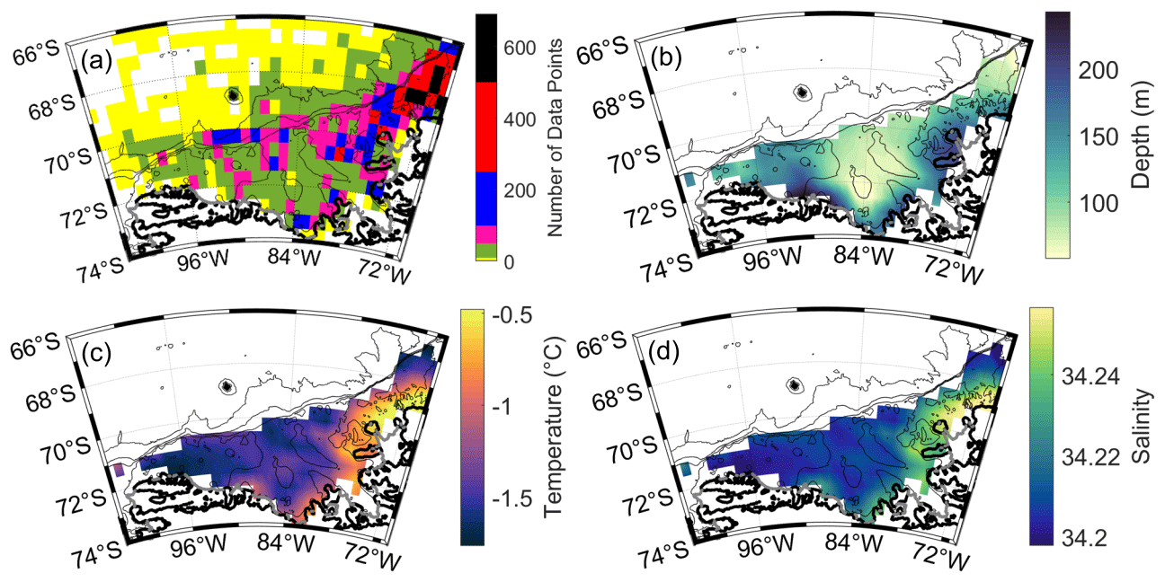
Figure 4Mean spatial distribution of winter water (WW) properties in the Bellingshausen Sea. The map is constructed using a grid spacing of 0.5∘ latitude and 1∘ longitude. (a) The number of data points within each grid cell (white represents a grid cell with no data). (b–d) Depth (meters), potential temperature (degrees Celsius), and salinity, respectively, on the 27.4 kg m−3 isopycnal.
3.1 Horizontal distributions
Due to the broad coverage of the seal profiles, this data set offers a unique opportunity to construct horizontal mean fields that may be constructed either along isobars or isopycnals. We focus on the latter in the following subsections. These maps provide a more complete picture of hydrographic variations than is typically permitted from discrete hydrographic sections (e.g., Castro-Morales et al., 2013). Summer melting of sea ice freshens and cools the surface layers, which, combined with heating later in the summer, forms the fresher and warmer seasonal thermocline. In the winter, sea ice formation increases salinity through brine rejection, resulting in mixing and deepening of the mixed layer. Thus, AASW shows the most variability in properties due to seasonal surface forcing variations (Whitworth et al., 1998). Our focus in the following is on layers below the surface, or water masses below AASW. We define these water masses based on density surfaces, which slightly differ over the span of the Bellingshausen Sea, to support our goal of describing how the properties change along the path of the AACC.
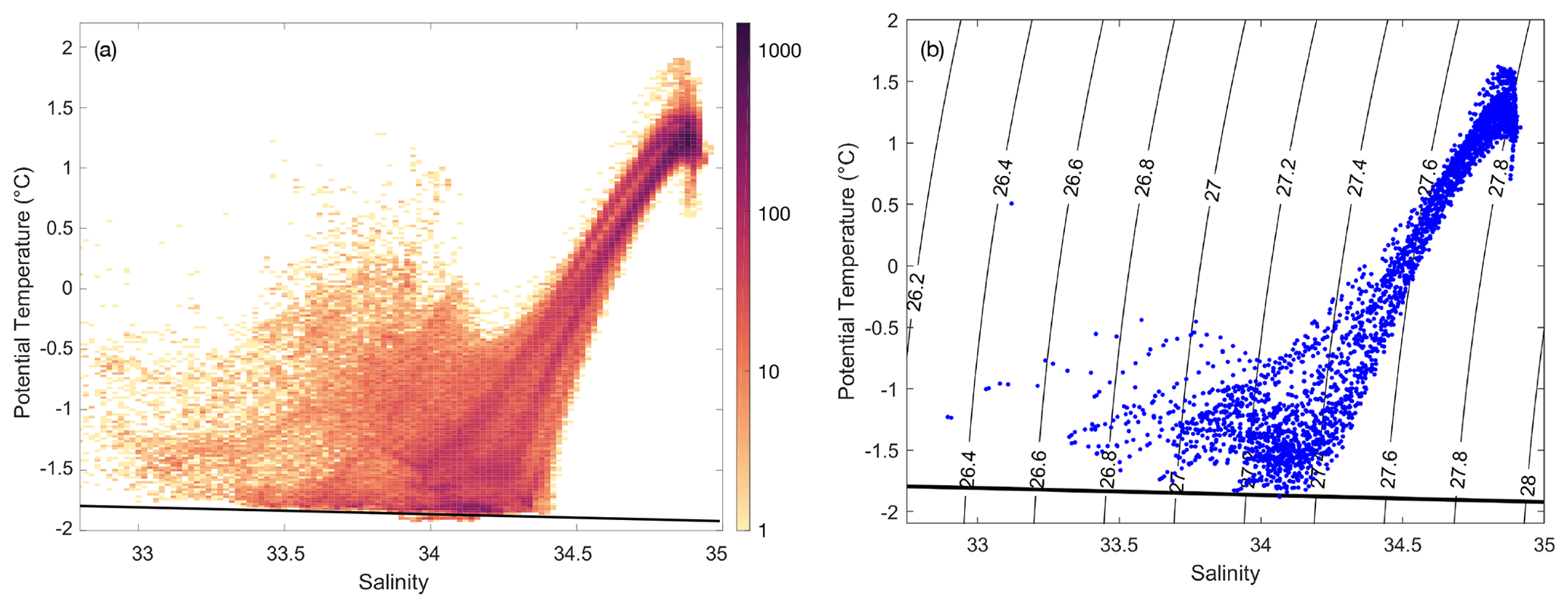
Figure 5Potential temperature–salinity plots as measured by instrumented seals in the Bellingshausen Sea. (a) A two-dimensional histogram of all the seal data over the continental shelf, using salinity and temperature intervals of 0.02 psu and 0.02 ∘C, respectively. The scale is logarithmic. (b) The distribution of potential temperature and salinity from the composite hydrographic sections is listed in Table 1. The thin black contour lines are of potential density. The thick black line is the freezing line.
3.1.1 Winter water
We illustrate the properties of the WW layer on the σ0=27.4 kg m−3 surface (Fig. 4b–d), with median values of isopycnal layer depth, temperature, and salinity taken from all available seal data. Properties of the continental shelf have been removed in panels (b–d) to better highlight variations over the continental shelf. Seasonal variations in the WW properties (divided into 6-month periods) are provided in the Appendix (Fig. A2). A key feature of the WW layer is its downward slope along the entire coast of the Bellingshausen Sea, indicating a baroclinic, westward geostrophic current, under the assumption that the velocity decays with depth (Fig. 4b). The shape of the 27.4 kg m−3 surface highlights the boundary-trapped nature of the AACC up to the western limit of the Bellingshausen Sea shelf, where the deeper excursion of the isopycnal surface extends away from the coast toward the shelf break. The offshore spatial gradient in the depth of the WW layer, calculated perpendicular to the coastline, appears as a narrow and relatively weak gradient in the east. The isopycnal depth gradient widens, and its magnitude increases south of the Wilkins Ice Shelf and into the central Bellingshausen Sea. The region of isopycnal tilt broadens again to the west in front of Abbot Ice Shelf. The potential temperature of the WW layer (Fig. 4c) is considerably warmer in the eastern Bellingshausen Sea as compared to the west, with a difference of roughly 1.15 ∘C.
Close to the coast, the temperature on this density surface is warmer than what is typically associated with WW, which may be due to upward mixing of warm CDW, as these regions are associated with large polynyas (Tamura et al., 2008). Lateral changes in temperature within the coastal boundary current are smaller, but the trend shows a consistent cooling from east to west. Similarly, the salinity of the WW layer varies, freshening from east to west, both broadly over the continental shelf and in the boundary current (Fig. 4d). The difference in the salinity from east to west has a magnitude of roughly 0.055. This cooling and freshening signal in the boundary current is related to an introduction of meltwater from the ice shelves in the Bellingshausen Sea.
Comparing summer and winter properties of the WW layer reveals that there are larger horizontal gradients in summer compared to the winter months (Fig. A2). Temperature, salinity, and isopycnal layer depth all have larger lateral gradients in summer than in winter in the region from 70∘ W to the George IV inlet. The temperature, on average, along the western front of the Wilkins Ice Shelf is roughly 0.2 ∘C higher in winter than in summer, and the salinity is roughly 0.015 psu greater in the winter than in the summer. The depth of the WW layer only varies by about 10 m between winter and summer. The smaller gradients from east to west in the winter could result from weaker advection from the AACC in the WAP. Moffat et al. (2008) defined the AACC as a strong coastal current in the summer, which weakens in winter. The AACC would provide an influx of warm, salty water into the Bellingshausen Sea in the summer, which would tend to strength gradients in summer, as compared to winter.
3.1.2 Transitional layer
On the σ0=27.65 kg m−3 layer that lies between the WW and CDW layers, the water is a mixture of WW, CDW, and glacial meltwater (Fig. A3). This layer roughly aligns with the pycnocline and the base of the AACC; thus, it is important to document its evolution along the coast. The horizontal gradient in isopycnal depth, perpendicular to the coast, has a similar pattern to this gradient in the WW layer. In the eastern Bellingshausen Sea, it is narrow and progressively becomes wider as the AACC moves along the Wilkins Ice Shelf. In the central Bellingshausen Sea, it again becomes narrow, but the magnitude increases before becoming wider again as the AACC exits the western Bellingshausen Sea. The potential temperature of the transitional layer (Fig. A3b) is warmer than the overlying WW layer, with warmer water in the east and colder water in the west, although the change in temperature from 70∘ W to the entrance of the George VI Ice Shelf is not as strong as for the WW layer, with a magnitude of roughly 0.54 ∘C. Instead, this layer has a more consistent shift to colder waters in the west. Salinity is higher in the east, at about 34.65, and transitions to lower values in the west, at about 34.61.
The differences between summer and winter months for the transition layer are similar to the WW layer (Fig. A3d–i). The temperature shows larger gradients in the Wilkins Ice Shelf region in summer compared to winter. The larger gradient in summer is due to warmer temperatures in the east, at around 72∘ W, compared to winter. In the east, the salinity gradients are larger in the summer than in the winter, where the salinity in the east is higher in summer compared to winter. The property changes between seasons are less clear farther to the west due to a lack of seal data.
3.1.3 Circumpolar deep water
Properties of the CDW layer are given by values interpolated onto the σ0=27.75 kg m−3 isopycnal (Fig. A4). This isopycnal slopes down towards the coast, similar to the WW and transitional layers (Fig. A4a). As in the other layers, this change in the depth of the isopycnal layer is much broader in the western Bellingshausen Sea, as compared to the central and eastern regions. The potential temperature in this layer is warmer and less variable than the overlying layers (Fig. A4), with a difference from east to west of only 0.22 ∘C. However, there is a large-scale spatial distribution with warmer waters in the east and cooler waters in the west. The modification of temperature and salinity within the boundary current is less evident in the CDW layer as compared to the WW and transitional layers, which again highlights the likely importance of meltwater leaving the ice shelf cavities at depths shallower than CDW (Schulze Chretien et al., 2021). A similar pattern can be seen in salinity, with saltier waters in the east and fresher waters in the west (Fig. A4), and a difference between these two regions of roughly 0.019. The near-absence of localized variability along the coast suggests that the AACC is less of a factor in water modification in this layer.
The CDW layer does not show notable differences between winter and summer months, consistent with this layer being largely isolated from surface forcing. In the east, the temperature in summer is slightly cooler than in winter; however, the gradients from east to west are of similar magnitude in both times of the year. Salinity variations between winter and summer are even weaker than temperature, although we note that the comparison of seasonal property changes in the western region of the Bellingshausen Sea is difficult due to the lack of observations in winter.
3.2 Vertical distributions
The composite hydrographic sections across the shelf of the Bellingshausen Sea are used next to display the median vertical structure of hydrographic properties. The overall vertical structure in each section is similar, starting with a more variable surface water layer, then a WW layer characterized by a temperature minimum, and below that a warm CDW layer that extends to the seafloor. Surface temperatures along each of the composite sections in the Bellingshausen Sea vary only slightly from the coast to the shelf break, whereas there is greater variability in surface temperatures in the eastern composite sections over the WAP continental shelf. Surface salinity variations are similar over both the Bellingshausen Sea and the WAP continental shelves, showing fresher water near the coast and saltier water near the shelf break. In total, seven hydrographic sections were constructed to show the evolution of properties and transports along the ice shelf front (Fig. 3). Note the change in scale for the different panels, to span the different distances, with the along-section distance indicated above the potential temperature. The 34.4 psu isohaline is also included in the geostrophic velocity panels in Fig. 9.
We used all available data for each composite section. Since there are considerably more data from winter months, the properties are more strongly weighted to winter seasons. For this reason, the distinction between AASW and WW water masses in each section is reduced. We begin by providing a detailed discussion of hydrographic section 3, which marks the eastern boundary of the Bellingshausen Sea and is largely representative of the other sections. For subsequent sections, we mainly highlight key differences from hydrographic section 3.
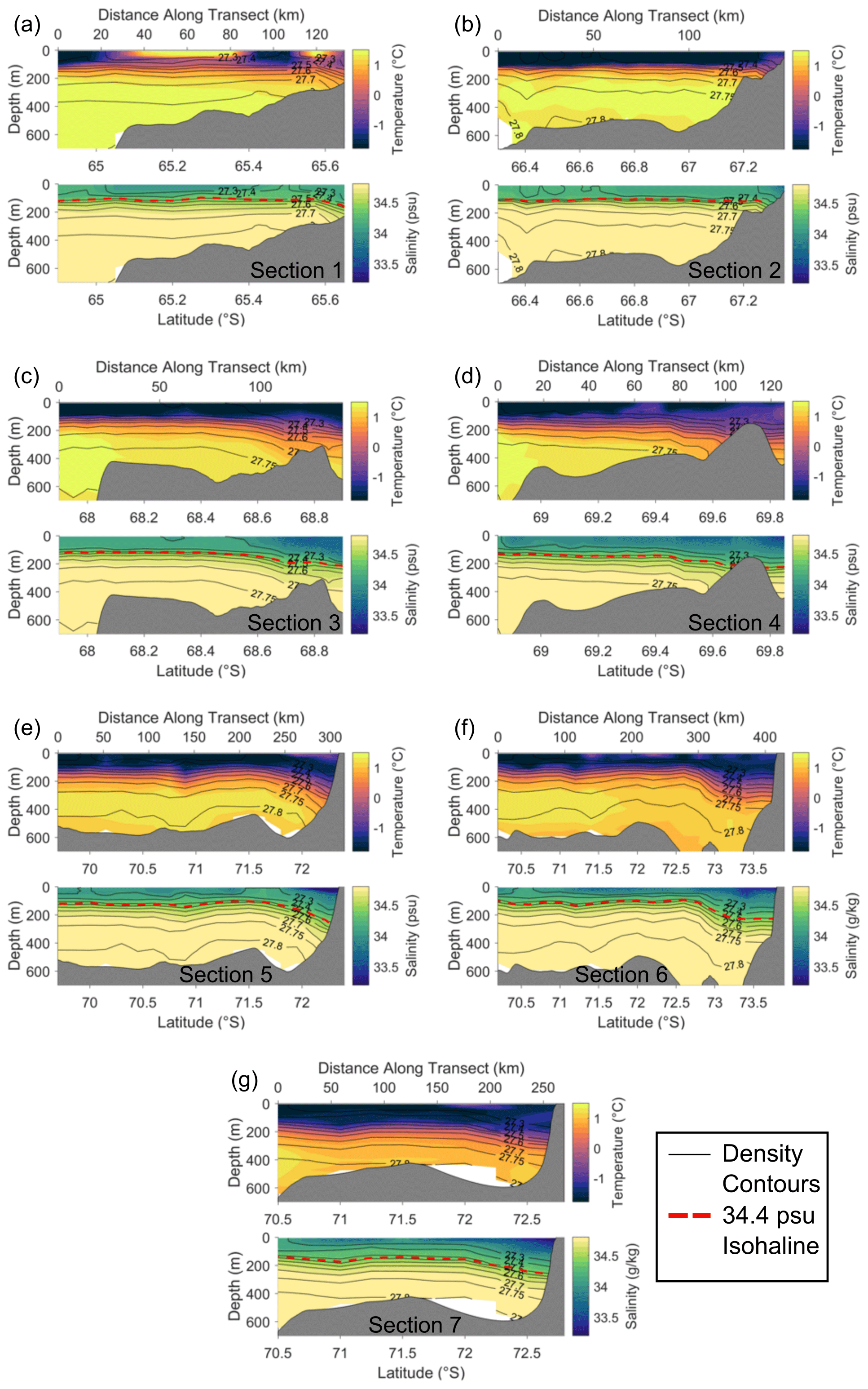
Figure 6Vertical hydrographic sections of potential temperature (top) and salinity (bottom) in the upper 700 m for each section in Fig. 3. Distance along the section is provided along the top of the temperature panels; note that sections are not of equal length.
Hydrographic section 3 (Fig. 6c) marks the boundary between the WAP continental shelf and the Bellingshausen Sea. This section is also located west of Marguerite Trough (Fig. 3, a key route for warm CDW to access the continental shelf and the northern extent of the George IV Ice Shelf (Venables et al., 2017; Brearley et al., 2019). In the composite section, the surface temperature varies only slightly from the coast to the shelf break (Fig. 6c), with an average temperature of −1.5 ∘C. In contrast to temperature, the surface salinity (Fig. 6c) shows substantial lateral variations along section 3, with a shallow fresh layer that extends from the coast to roughly 68.6∘ S, increasing from 33.7 psu near the coast to 34 psu near the shelf break. Below this surface layer, the vertical (composite) stratification peaks at roughly 150 m depth. The vertical stratification is set by the salinity as temperature increases almost uniformly throughout the water column, increasing from −1.4 ∘C above the halocline to 0.5 ∘C below the halocline. At the shelf break, near 68∘ S, a warm core of CDW is found between 250 and 500 m, with temperatures exceeding 1.5 ∘C. This structure is consistent with warm waters observed over the shelf modified from offshore sources through some combination of mixing processes, surface forcing, and interactions with ice shelves.
Isopycnals are aligned with salinity contours and are nearly flat offshore of 68.4∘ S. Onshore of this latitude, the salinity and the density contours slope down towards the coast. This downward tilt of the isopycnals is a common feature across all the composite sections and gives rise to the baroclinic structure of the AACC flowing southwestward in the WAP and westward in the Bellingshausen Sea.
The easternmost section (section 1; Fig. 6a) shows two near-surface cores of warm water with temperatures exceeding 1 ∘C. These cores are bounded by colder waters where the surface approaches the freezing temperature. Section 1 is the only composite section where summertime profiles exceed the number of wintertime profiles, which is why surface temperatures are warmer than other sections. The salinity shows surface variations, initially fresher at 34 psu and increasing to 34.2 psu at the first temperature minimum. The potential density contours of 27.3 and 27.4 kg m−3 extend towards the surface (Fig. 6a) at the temperature minima. This structure is likely a remnant of winter ice freezing on the shelf. Below the surface layer, the temperature is more uniform across the shelf and shelf break compared to hydrographic section 3 (Fig. 6a). Beneath the thermocline, the temperature is close to 1.3 ∘C across the entire section, increasing to about 1.5 ∘C at the bottom. Salinity increases from 34.5 psu at the top of the halocline to 34.7 psu at the bottom of the halocline. The salinity reaches a maximum of roughly 34.8 psu at the bottom. Density follows the salinity and slopes down towards the coast near 65.55∘ S. This structure is similar to the hydrographic sections presented in Moffat et al. (2008).
Hydrographic section 2 (Fig. 6b) shows structure more typical of the water column over the rest of the shelf. The surface mixed layer, consisting of AASW and WW, shows a temperature minimum from about 67.25∘ S to the northern extent of the section. From 67.25∘ S, the temperature increases from −1.8 to −1.28 ∘C at the coast. Near the coast the salinity is 33.71 psu and increases to 34.1 psu at 67.25∘ S. North of this latitude, the salinity varies between 34.1 and 34.2 psu, with maximum values close to the shelf edge. The thermocline and halocline occur around 125 m depth. The temperature profile beneath the thermocline increases to an average maximum temperature of 1.4 ∘C at 400 m. Pockets of warmer water exist in cores around 400 m, reaching 1.52 ∘C. The salinity below the halocline increases from about 34.65 to 34.75 psu at the bottom. The density on level surfaces decreases towards the coast at roughly 67.25∘ S, indicating the presence of the AACC.
Moving west of section 3, into the Bellingshausen Sea shelf region, the temperature near the surface appears warmer, particularly near the coast. The salinity at the surface progressively decreases, and this fresher water extends farther away from the coast. We believe that this occurs due to the continued entrainment of meltwater by the AACC from the melting ice shelves (Schulze Chretien et al., 2021). The thermocline and halocline are found at somewhat deeper levels, from a depth of 150 m in section 3 to a depth of 200 m in section 7. The isopycnal tilt near the coast strengthens somewhat from east to west but, more importantly, extends to a greater distance away from the coast, indicating that the baroclinic portion of the AACC intensifies (Sect. 4).
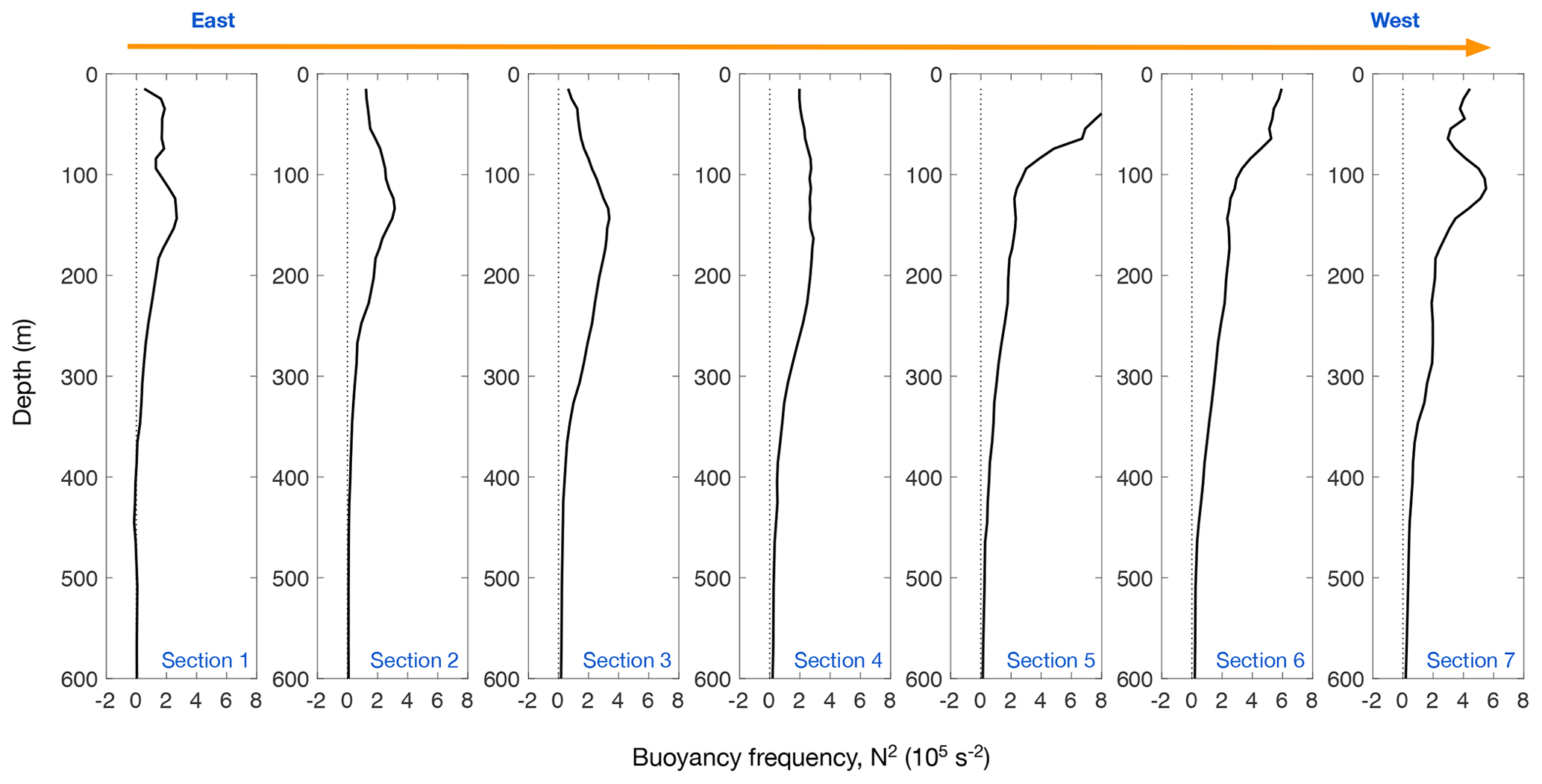
The vertical structure of properties is important for understanding the evolution of the AACC. At the surface, the temperature becomes slightly warmer near the coast, but the most noticeable change is a reduction in salinity, which has a larger effect on density. The thermocline and halocline are depressed and found deeper in the west compared to in the east. The vertical stratification near the coast also undergoes an evolution from east to west (Fig. 7). Over the WAP shelf (sections 1–3), the stratification, given in terms of the buoyancy frequency , where g is gravity, and ρ0=1027 kg m−3 is a reference density, peaks at a value of s−2 at a depth of 150 m. Once entering the Bellingshausen Sea, the AACC stratification changes in two important ways; first, the near-surface (upper 100 m) becomes much more stratified, and the stratification deepens with N2 exceeding s−2 below 300 m in sections 6 and 7 (Fig. 7). The increase in surface stratification due to freshening points to an influx of freshwater either from runoff, sea ice melt, or buoyant meltwater convection near the face of ice shelves. The deeper change in the stratification is likely due to the outflow of glacially modified CDW and marks the base of the AACC (Ruan et al., 2021; Schulze Chretien et al., 2021).
From the hydrographic data discussed in Sect. 3, a dynamic height field was constructed in the Bellingshausen Sea, showing the surface values relative to 400 m depth. Dynamic height is elevated near the coast throughout the Bellingshausen Sea (Fig. 8), consistent with a pressure gradient directed offshore, and balanced by the Coriolis force to support a mean, near-surface, westward, along-coast flow. This flow is discussed in more detail below by constructing composite sections of geostrophic velocity (Fig. 9). In the eastern Bellingshausen Sea, dynamic height indicates that a coastal flow enters from the WAP as a narrow boundary current. The value is largest near the coast and changes by 0.6 m2 s−2 across an offshore distance of roughly 100 km. As the AACC flows around the Wilkins Ice Shelf, the region of strong dynamic height gradient widens to 140 km, but the difference in dynamic height increases to 0.8 m2 s−2. In the central Bellingshausen Sea, the region of strong dynamic height gradient becomes narrower, occupying a region of only 70 km, and the difference in dynamic height across this boundary current continues to increase to 0.9 m2 s−2. Here the velocity of the AACC has its greatest magnitude in the Bellingshausen Sea. The difference in dynamic height across the boundary current continues to increase through the Venable Ice Shelf, until, on its western side, the region of strong gradient widens to over 200 km with a difference of 0.8 m2 s−2. West of the Venable Ice Shelf, the dynamic height contours suggest that the path of the AACC divides, with some component of the flow directed toward the shelf break and another component along the face of the Abbot Ice Shelf.

Figure 8Spatial map of surface dynamic height (square meters per second; m2 s−2), referenced to 400 m. The red contours have an interval of 0.2 m2 s−2.
We next use the composite hydrographic sections to construct geostrophic velocities perpendicular to the section and, therefore, largely oriented parallel to the shelf break and the coastline. Figure 9 shows the geostrophic velocity and cumulative volume transport for each of the hydrographic sections (negative values are directed westward). The transport is calculated by integrating the velocities with respect to depth between the 34.4 isohaline and the surface and with distance from the coast, such that the transport at the outer limit is equivalent to the net along-shelf volume transport in Sverdrups (1 Sv=106 m3 s−1). Table 2 summarizes the results for each of the seven hydrographic sections.
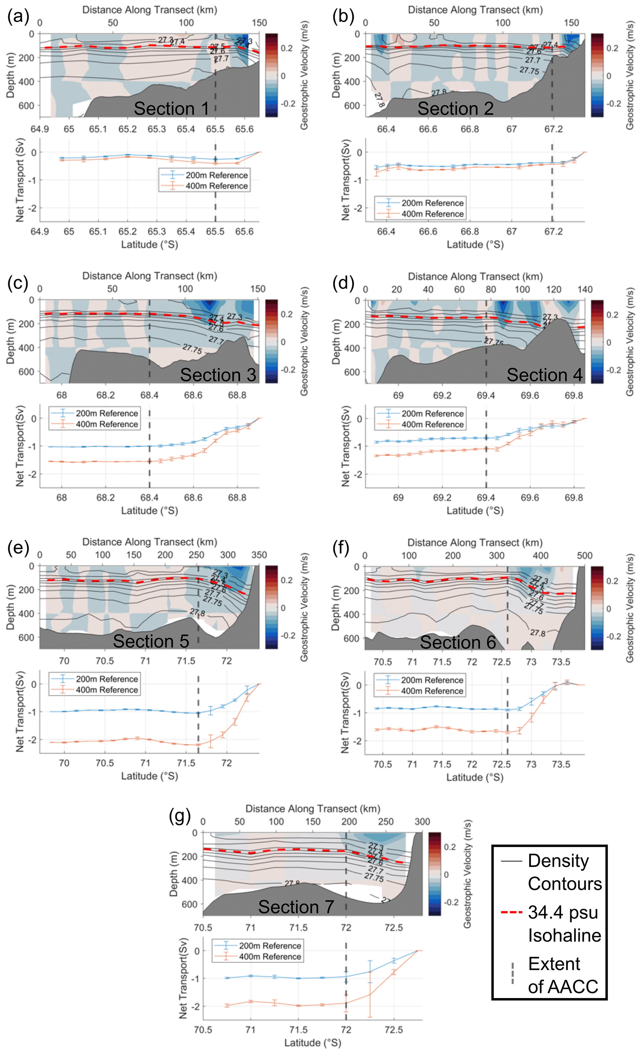
Figure 9Geostrophic velocity (meters per second – m s−1; referenced to 400 m; top) and geostrophic transport (Sv; bottom) for all sections in Fig. 3. Transport values are given for both the 200 and 400 m reference level, and transports are cumulative from the coast and calculated by integrating from the surface to the 34.4 psu isohaline (red dashed curve). Negative (positive) values indicate westward (eastward) transport and flow.
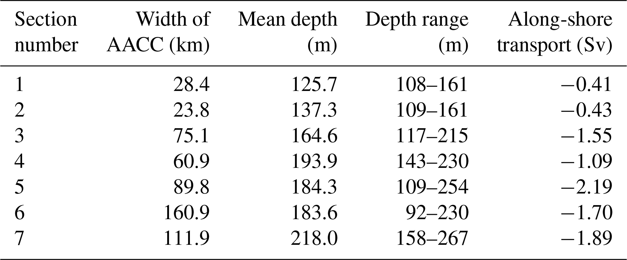
Table 2Width (kilometers), mean depth (meter), range of depth (meters) and along-shore transport for the AACC in each of the seven hydrographic sections shown in Fig. 3.
In order to arrive at an absolute geostrophic velocity, a reference level of no motion must be selected. Here, we apply a 200 m reference level of no motion to calculate the volume transports for sections 1–3 and compare these to the volume transport calculated by Moffat et al. (2008), located between sections 1 and 2, and shown in Fig. 10a. Section 1 (Figs. 3 and 10a), located to the north and east of the Moffat et al. (2008) section, has a transport of Sv. Recall that these transports represent the flow confined to the AACC as determined by the location where depth-integrated velocity is 15 % of the value at the center of the current (see Sect. 2.3 and the vertical dashed lines in Fig. 9). Section 2 is located to the south and west of the Moffat et al. (2008) section, and the transport is Sv. For comparison, the transport of the Moffat et al. (2008) section was reported to be Sv. Moving along the coast to the west, volume transports increase. Jenkins and Jacobs (2008) found that a transport of −0.24 Sv flows south through the Marguerite Trough. This additional transport explains a jump in transport between our sections 2 and 3, where, in the latter section, the AACC transport is Sv. The comparison with the estimate from Moffat et al. (2008), using a 200 m reference level, gives us confidence that our velocity and transport estimates are reasonable. For the remainder of the section, we will report geostrophic velocities and transports using a 400 m reference level, as discussed in Sect. 2.3.
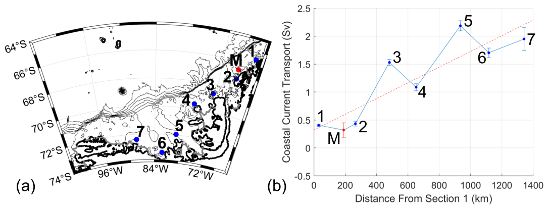
Figure 10(a) Location of AACC transport estimates based on the hydrographic transects labeled as in Fig. 3, and (b) the values of transport (Sv; 1 Sv=106 m3 s−1) along the AACC. The transport increases as the AACC flows westward. The transport estimate from Moffat et al. (2008) in the WAP is included in both panels and indicated by the red dot labeled M. All of the transport values, except for the Moffat et al. (2008) section, are with respect to a level of no motion at 400 m. The red dashed line shows a linear trend of 2 Sv per 1000 km. The blue dots in panel (a) indicate the midpoint of the AACC in each section.
Throughout the WAP and Bellingshausen Sea there is westward flow along the coast. The extent of the AACC is defined as the region between the coast and the location where depth-integrated velocity is 15 % of the value at the center of the current, indicated by the vertical dashed lines in Fig. 9. In section 1, the geostrophic velocity in the AACC has a peak value of −0.21 m s−1 and an average velocity of −0.06 m s−1. Section 2, similarly, shows the AACC tightly confined to the coast, with a similar peak westward velocity of −0.20 m s−1 and an average of −0.057 m s−1. The peak velocities in sections 1 and 2 are similar to the surface velocities found in the fall by the mooring in (Moffat et al., 2008), which they found to range from −0.15 to −0.20 m s−1. Across section 3, the first section in the Bellingshausen Sea, the velocity of the AACC has an average value of −0.056 m s−1, with a maximum value of −0.26 m s−1. Here, the AACC occupies a much larger area than in the previous sections (Fig. 9c). In section 4, the average velocity decreases to −0.04 m s−1, and the maximum velocity is −0.26 m s−1. The decrease in average velocity in section 4 is associated with the current splitting into three different cores seen in Fig. 9d. As the AACC enters into the central Bellingshausen Sea, the average velocity increases, in section 5, to −0.05 m s−1. The velocity maximum in this section is −0.20 m s−1, which is a decrease in magnitude from the previous two sections. The next section sees the average velocity decrease to −0.026 m s−1 and a maximum velocity of −0.11 m s−1. The final section, section 7 in the western Bellingshausen Sea, has an average velocity of −0.041 m s−1 and a maximum of −0.12 m s−1. As we discuss below, part of the variability in the average geostrophic velocity is tied to a broadening of the AACC that is better captured by the changing geostrophic transport.
The magnitude of the geostrophic velocity is variable across the various composite sections, which could result from a number of factors, including surface forcing effects (modifying the sea surface height) and width of the AACC. Note that the “average” velocity across the AACC, reported above, was selected as a simple diagnostic of the flow and should be interpreted with some caution. Even with the weak stratification of the waters on the Antarctic continental shelf, the AACC may be tied to flow over particular isobaths as it reaches a geostrophic equilibrium where offshore Ekman transport of the boundary current at the bottom is zero (Lentz and Helfrich, 2002). If the current moves offshore to follow a particular isobath, the AACC would appear wider, even if the core remains narrow (e.g., section 4). The along-coast transport, on the other hand, provides a clearer picture of the evolution of the AACC. The striking feature is a nearly linear trend in volume transport extending from the WAP through the western Bellingshausen Sea. Values along the WAP show that the AACC carries roughly 0.5 Sv of transport, which increases to more than 1 Sv in the eastern Bellingshausen Sea and is ultimately close to 2 Sv in the western Bellingshausen Sea (Fig. 10). Using a Monte Carlo error analysis, we also estimated error bars for the transport (shown as vertical bars in Fig. 10), supporting the presence of a significant trend.
Throughout the Bellingshausen Sea continental shelf, the density structure near the coast is consistent with a baroclinic, vertically sheared flow that is westward near the surface. Additionally, the lateral density gradients intensify and extend further away from the coast as the AACC moves towards the west, suggesting a strengthening of the AACC. Thus, the evolution of the AACC, inferred from hydrographic properties through dynamic height, geostrophic velocity, and transport estimates, shows a consistent picture of a connected circulation feature that extends from the WAP through the western Bellingshausen Sea.
The Bellingshausen Sea region shows higher salinities and temperatures in the east near the surface, whereas, toward the west, both temperature and salinity decrease. This change can be attributed to the following two processes: (i) the enhanced basal melting in the ice shelf cavities of the Bellingshausen Sea that produces more meltwater, and (ii) the circulation in the AACC and the accumulation of meltwater as the AACC flows westward. The basal melt rates of Bellingshausen Sea ice shelves are amongst the highest throughout Antarctica (Paolo et al., 2015; Walker and Gardner, 2017; Adusumilli et al., 2020), which introduces meltwater mixtures with a lower temperature and salinity. Polynyas, associated with brine rejection due to sea ice formation, persist almost year round but do not lead to penetrative convection to the seafloor (Tamura et al., 2008; Holland et al., 2010). However, there is not an accompanying increase in salinity from east to west that would be associated with accumulating brine rejection in areas of sea ice formation. The increased salinity from ice formation in polynyas, where they are present, counteracts to some extent the decrease seen in salinity from east to west. But this effect is overwhelmed by the entrainment of glacial meltwater. Local sea ice variability may also play a factor in modifying the properties of the water through ocean–atmosphere heat fluxes (Walker and Gardner, 2017).
The density field is consistent with a dominant baroclinic structure of the AACC. The geostrophic velocities in Fig. 9 provide details of the AACC flow. As the AACC transitions from the WAP to the Bellingshausen Sea, the transport increases as the warm water below the current enters the ice cavity and produces meltwater, creating a plume of entrained CDW which, in turn, feeds the along-shore flow. The average velocity of the AACC remains relatively constant in the transition from the WAP to the eastern Bellingshausen Sea. Within the central and western Bellingshausen Sea, the average velocity varies from section to section, but a widening of the AACC causes the transport to steadily increase. Wind forcing may also influence the AACC structure and is coupled to the presence of almost year-round polynyas near the coast (Assmann et al., 2005; Holland et al., 2010). However, the strength and orientation of the wind stress close to the coast is not well determined due to the lack of observations to validate reanalysis products. The introduction of meltwater from the melting ice shelves is the most likely explanation for the growing transport of the AACC, consistent with the observed along-coast trends in temperature and salinity.

Figure 11Drifter tracks for two drifters released as part of the Long Term Ecological Research (LTER) program and offering additional support that the AACC provides a connection between the WAP and the Amundsen Sea. Drifter 54 160 was released on 1 January 2007 and recorded positions through 24 December 2007. Drifter 70 579 recorded positions between 27 January and 24 November 2007; there is a gap in the data for this drifter during 18–27 May (around 74∘ W). Large black dots indicate the beginning and end of each drifter track.
Independent evidence provided by surface drifters provides further support for a continuous coastal current that spans the Bellingshausen Sea; surface drifter trajectories were also key in early studies that identified the AACC along the WAP (Beardsley et al., 2004). Figure 11 shows the tracks of two surface drifters that were released in 2007 as part of the Long Term Ecological Research (LTER) program (https://scienceweb.whoi.edu/coastal/LTER_Drifter/index.html, last access: 4 February 2021). Both of these drifters show a westward flow pattern consistent with a continuous AACC. These drifters provided high-frequency position fixes with a separation of only about 27 min; we have not averaged the data. Drifter 54 160, (blue curve in Fig. 11) was released in the eastern Bellingshausen Sea and was advected into the eastern Amundsen Sea before it stopped sending back data. This drifter was deployed on 1 January 2007 and reached the central Bellingshausen Sea, defined here as 82.5∘ W, on 15 March with an average speed over that time span of 0.30 m s−1. This drifter then reached the Abbot Ice Shelf, defined as crossing 91.5∘ W, on 28 March. The average speed of drifter 54 160 during this stretch of time was 0.41 m s−1. The drifter then entered into the Amundsen Sea, providing at least anecdotal evidence that the AACC in the Bellingshausen Sea is connected to the Amundsen Sea. The last recording for drifter 54 160 was on 24 December in the Amundsen Sea. From 28 March to 24 December, the average speed was 0.22 m s−1. Drifter 70 579, in red, was released near the coast on the WAP on 21 January 2007 and then entered into the eastern Bellingshausen Sea, defined as crossing 71∘ W, on 9 March with an average velocity of 0.38 m s−1 over that time span. There was a gap in the drifter data between 18 and 27 May, but the velocity between the two data points that are on either side of the gap was 0.15 m s−1. The final data point for drifter 70 579 is 24 November in the central Bellingshausen Sea. The average velocity from 27 May to 24 November was 0.26 m s−1. It is notable that these drifters persisted for nearly 12 months, suggesting that an open-water pathway along the coast is maintained over much of the year.
The AACC could have as many as three separate pathways from the Bellingshausen Sea into the Amundsen Sea. First, near the Venable Ice Shelf and the eastern extent of the Abbot Ice Shelves, a branch of the AACC appears to deflect to the north, likely steered by topography on the western side of the Belgica Trough, and flows offshore where it eventually joins the ASF. Observations over the continental shelf and slope suggest that this is the primary route for the export of meltwater from the Bellingshausen Sea (Thompson et al., 2020; Schulze Chretien et al., 2021), and once part of the ASF, these waters may flow along the shelf break into the Amundsen Sea (Mallett et al., 2018; Thompson et al., 2020). An alternative route of the AACC is to continue along the coast in front of the Abbot Ice Shelf. Here two possibilities present themselves: (i) flow along the ice shelf face and around Thurston Island or (ii) flow under the Abbot Ice Shelf and into the eastern Amundsen Sea. The path around Thurston Island is described by drifter 54 160 (Fig. 11) and may be the more likely route since the AACC is largely a surface-trapped feature, shallower than the draft of the Abbot Ice Shelf. If part of the AACC were to flow under the Abbot Ice Shelf, it would re-emerge from under the ice shelf considerably further south in the Amundsen Sea and contribute to water properties that interact with the Pine Island and Thwaites ice shelves. Much farther downstream, evidence for the influence of the AACC, beyond the Amundsen, is suggested by heat and fresh water budgets on the shelf in the Ross Sea. In particular, Porter et al. (2019) note that a flux of cool water into the Ross Sea is provided by the AACC; this was also noted by Orsi and Wiederwohl (2009).
Using hydrographic data collected from seals equipped with CTD-SRDLs, the structure of the coastal circulation in the Bellingshausen Sea and the southern WAP were investigated. The observations were used to produce maps on density layers to understand the horizontal distribution of physical properties. The vertical distribution of properties was investigated by creating multiple composite hydrographic sections, spanning the coast to the shelf break, which reveal a steady evolution of coastal properties between the WAP and the western Bellingshausen Sea.
Along the coast, there is a consistent cooling and freshening trend from east to west in the upper 200 m of the water column. Additionally, the pycnocline deepens progressively across these sections from the WAP to the western Bellingshausen Sea, which we attribute to an entrainment of glacial meltwater. The meltwater fills an upper, buoyant layer and depresses the thermocline and halocline along with the warmer, saltier water below. The deepening on this pycnocline enhances local lateral density gradients, resulting in a stronger AACC with a greater volume transport, which increases from 0.5 Sv along the WAP to roughly 2 Sv in the western Bellingshausen Sea.
The large number of hydrographic profiles also allowed us to map the large-scale structure of the AACC using dynamic height. This product reveals that the AACC in the Bellingshausen Sea is connected to both the WAP in the east (what has previously been referred to as the Antarctic Peninsula Coastal Current in Moffat et al., 2008) and the Amundsen Sea to the west. The inflow into the Bellingshausen Sea from the north is confined to a narrow southward-flowing boundary current along the coast, an orientation that is opposite to the northeastward flow of the AACCs southern boundary at the shelf break. The pathway of the AACC out of the Bellingshausen Sea to the west is less clear. In the western Bellingshausen Sea, the flow at the shelf break has a westward component (Nakayama et al., 2014; Thompson et al., 2020), such that both coastal and shelf break routes of the AACC towards the Amundsen may be possible. The increase in volume transport of the AACC is likely due to changes in stratification linked to the addition of meltwater flowing out of ice shelf cavities. The direct input of meltwater itself is too small to account for the increased volume transport of the AACC, but the entrainment of waters flowing on to the Bellingshausen Sea continental shelf and towards the coast, within the Latady and Belgica troughs, supplies much of the mass that upwells under the ice shelves (Thompson et al., 2020; Schulze Chretien et al., 2021).
The AACC emerges as a key component of the larger cyclonic West Antarctic circulation system that connects the WAP, Bellingshausen, Amundsen, and Ross seas. As meltwater is introduced into the AACC, the near-surface temperature and salinity decreases, and the vertical stratification is also modified. These changes can feed back on a number of processes, i.e., surface fluxes in polynyas, the formation of sea ice, and vertical and lateral heat and freshwater fluxes within the water column. These implications highlight the need for further consideration of both local and nonlocal impacts of enhanced meltwater input into the AACC, especially for the lateral heat transport towards ice shelves and for bottom water formation rates.
In this Appendix, we provide additional figures to support and expand upon the results in the main text. Figure A1 shows an expanded view of the seal data that were used in this study that include data from the WAP (Fig. 4). The dots in blue are the same as the ones displayed in Fig. 2. Figures A2–A4 provide additional background on the seasonal cycle of properties compared to the typical (median) conditions. We present these figures in this Appendix since they help to provide the broader context for the key results presented in the main text.
Figure A2 complements Fig. 4 by separating the properties of WW (27.4 kg m−3 density surface) into summer (October–March) and winter (April–September) months. The main results of this figure are discussed in the main text. Figures A3 and A4 also show a seasonal decomposition on the transition layer and CDW layer (27.65 and 27.75 kg m−3 density surfaces, respectively). Only the mean WW properties are presented in the main text because this is where the largest along-isopycnal gradients are found in hydrographic properties. Therefore, Figs. A3 and A4 include panels to show the median values as described previously.
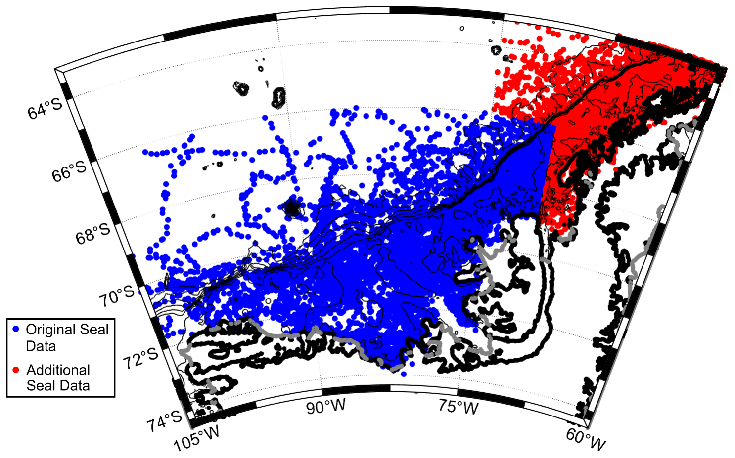
Figure A1Map showing the position of hydrographic profiles from the instrumented seals divided into the Bellingshausen Sea (blue) and the West Antarctic Peninsula (red). The red data include an additional 10 074 profiles separate from those in Fig. 2 that were used to construct composite hydrographic sections 1 and 2 (Fig. 3).
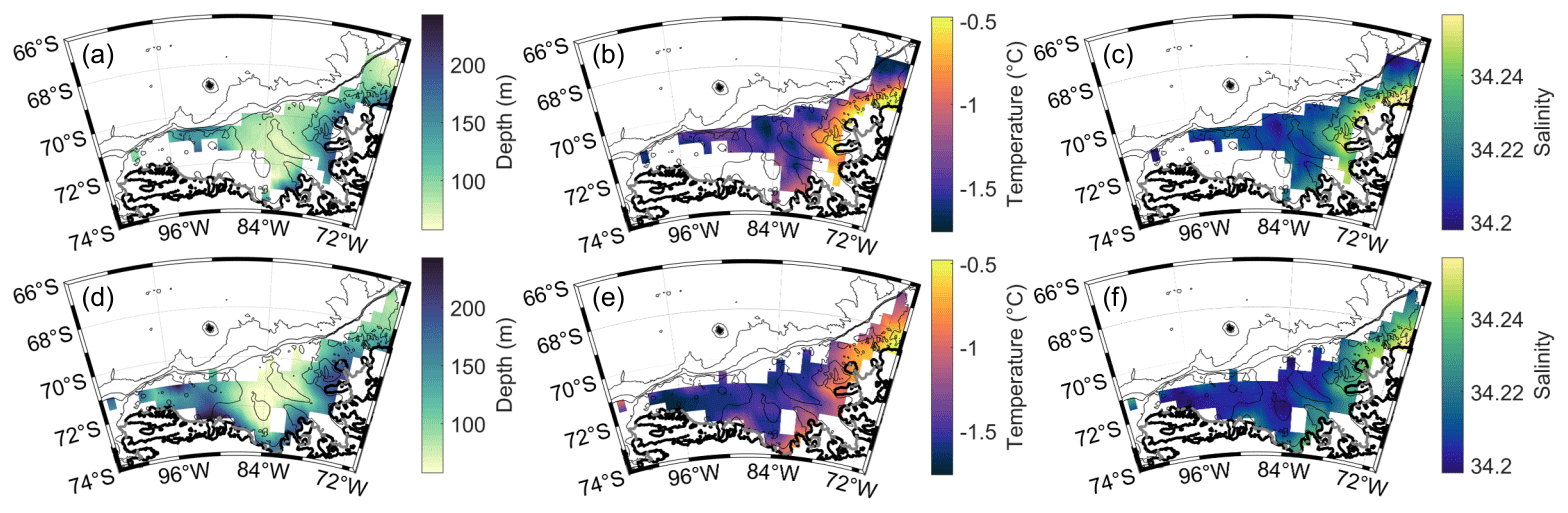
Figure A2The distribution of properties on the WW potential density layer (σ0=27.4 kg m−3), divided into (a–c) winter (April–September) and (d–f) summer (October–March) months. (a, d) Depth of the density layer (meters), (b, e) potential temperature (degrees Celsius), and (c, f) salinity are shown.
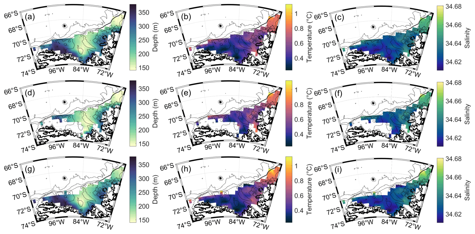
Figure A3The distribution of properties on the transitional potential density layer (σ0=27.65 kg m−3), divided into (a–c) median, (d–f) winter (April–September), and (g–i) summer (October–March) months. (a, d, g) Depth of the density layer (meters), (b, e, h) potential temperature (degrees Celsius), and (c, f, i) salinity are shown.
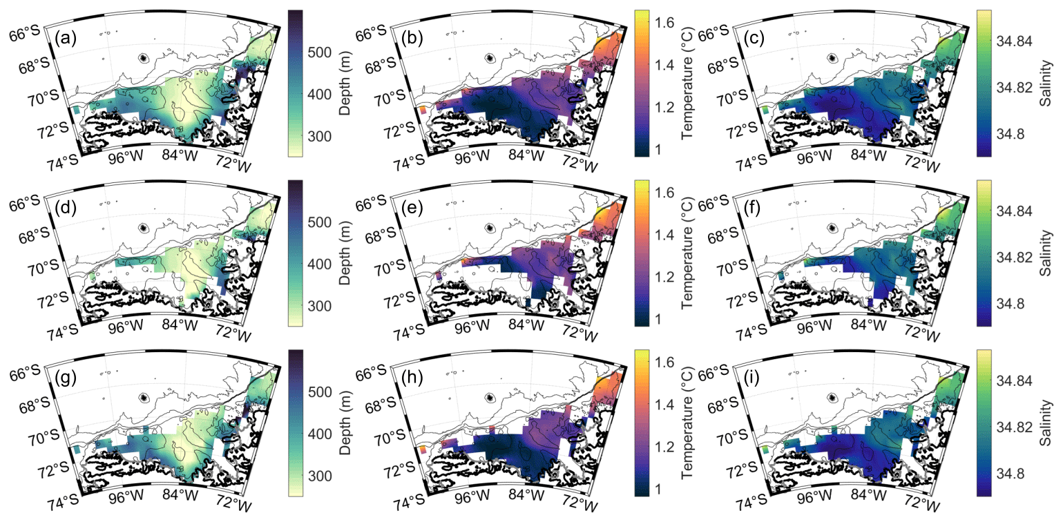
Figure A4The distribution of properties on the CDW potential density layer (σ0=27.75 kg m−3), divided into (a–c) median, (d–f) winter (April–September), and (g–i) summer (October–March) months. (a, d, g) Depth of the density layer (meters), (b, e, h) potential temperature (degrees Celsius), and (c, f, i) salinity are shown.
All analysis and figures were created using MATLAB. Analysis scripts are available upon request from Ryan Schubert. The instrumented seal data were obtained from the publicly available MEOP database, which can be found at https://meop.net/database/meop-databases/density-of-data.html (Treasure et al., 2017).
KS and AFT conceived and designed the study. RS performed the analysis and wrote the paper. YB and LSC assisted with the data analysis.
The authors declare that they have no conflict of interest.
Publisher's note: Copernicus Publications remains neutral with regard to jurisdictional claims in published maps and institutional affiliations.
We gratefully acknowledge all of the scientists who have contributed to the MEOP project through their seal tagging and data processing efforts. In particular, we thank Fabien Roquet, who assisted with processing of the seal data previously. The marine mammal data were collected and made freely available by the International MEOP Consortium and the national programs that contribute to it (http://www.meop.net, last access: 31 September 2021).
This research has been supported by the Office of Polar Programs (grant nos. 1643679 and 1644172) and the Division of Ocean Sciences (grant no. 1658479).
This paper was edited by Nicolas Jourdain and reviewed by two anonymous referees.
Adusumilli, S., Fricker, H. A., Medley, B., Padman, L., and Siegried, M. R.: Interannual variations in meltwater input to the Southern Ocean from Antarctic ice shelves, Nat. Geosci., 13, 616–620, 2020. a, b
Assmann, K., Hellmer, H. H., and Jacobs, S. S.: Amundsen Sea ice production and transport, J. Geophys. Res., 110, C12013, https://doi.org/10.1029/2004JC002797, 2005 a, b, c, d
Beardsley, R. C., Limeburner, R., and Owens, W. B.: Drifter measurements of surface currents near Marguerite Bay on the western Antarctic Peninsula shelf during austral summer and fall, 2001 and 2002, Deep-Sea Res. Pt. II, 51, 1947–1964, 2004. a
Brearley, J. A., Moffat, C., Venables, H. J., Meredith, M. P., and Dinniman, M. S.: The role of eddies and topography in the export of shelf waters from the West Antarctica Peninsula shelf, J. Geophys. Res., 124, 7718–7742, 2019. a
Bronselaer, B., Winton, M., Griffies, S. M., Hurlin, W. J., Rodgers, K. B., Sergienko, O. V., Stouffer, R. J., and Russell, J. L.: Change in future climate due to Antarctic meltwater, Nature, 564, 53–58, 2018. a
Castro-Morales, K., Cassar, N., Shoosmith, D. R., and Kaiser, J.: Biological production in the Bellingshausen Sea from oxygen-to-argon ratios and oxygen triple isotopes, Biogeosciences, 10, 2273–2291, https://doi.org/10.5194/bg-10-2273-2013, 2013. a, b
Dutrieux, P., De Rydt, J., Jenkins, A., Holland, P. R., Ha, H. K., Lee, S. H., Steig, E. J., Ding, Q., Abrahamsen, E. P., and Schröder, M.: Strong sensitivity of Pine Island ice-shelf melting to climatic variability, Science, 343, 174–178, 2014. a
Efron, B. and Tibshirani, R. J.: An introduction to the bootstrap, CRC press, Boca Raton, Florida, 1994. a
Golledge, N. R., Keller, E. D., Gomez, N., Naughten, K. A., Bernales, J., Trusel, L. D., and Edwards, T. L.: Global environmental consequences of twenty-first-century ice-sheet melt, Nature, 566, 65–72, 2019. a
Heywood, K. J., Naveira Garabato, A. C., Stevens, D. P., and Muench, R. D.: On the fate of the Antarctic Slope Front and the origin of the Weddell Front, J. Geophys. Res.-Oceans, 109, C06021, https://doi.org/10.1029/2003JC002053, 2004. a
Holland, P. R., Jenkins, A., and Holland, D. M.: Ice and ocean processes in the Bellingshausen Sea, Antarctica, J. Geophys. Res., 115, C05020, https://doi.org/10.1029/2008JC005219, 2010. a, b, c, d, e, f, g
Holland, P. R., Bracegirdle, T. J., Dutrieux, P., Jenkins, A., and Steig, E. J.: West Antarctic ice loss influenced by internal climate variability and anthropogenic forcing, Nat. Geosci., 12, 718–724, 2019. a
Jenkins, A. and Jacobs, S.: Circulation and melting beneath George VI ice shelf, Antarctica, J. Geophys. Res, 113, C04013, https://doi.org/10.1029/2007JC004449, 2008. a, b, c
Jenkins, A., Shoosmith, D., Dutrieux, P., Jacobs, S., Kim, T. W., Lee, S. H., Ha, H. K., and Stammerjohn, S.: West Antarctic Ice Sheet retreat in the Amundsen Sea driven by decadal oceanic variability, Nat. Geosci., 11, 733–738, 2018. a
Kim, C.-S., Kim, T.-W., Cho, K.-H., Ha, H. K., Lee, S., Kim, H.-C., and Lee, J.-H.: Variability of the Antarctic Coastal Current in the Amundsen Sea, Estuar. Coast. Shelf S., 181, 123–133, 2016. a, b, c
Kimura, S., Jenkins, A., Regan, H., Holland, P. R., Assmann, K. M., Whitt, D. B., Wessem, M. V., van de Berg, W. J., Reijmer, C. H., and Dutrieux, P.: Oceanographic controls on the variability of ice-shelf basal melting and circulation of glacial meltwater in the Amundsen Sea Embayment, Antarctica, J. Geophys. Res., 122, 10,131–10,155, 2017. a, b, c
Lentz, S. J. and Helfrich, K. R.: Buoyant gravity currents along a sloping bottom in a rotating fluid, J. Fluid Mech., 464, 251–278, 2002. a
Mallett, H. K. W., Boehme, L., Heywood, K. J., Stevens, D. P., and Roquet, F.: Variation in the distribution and properties of circumpolar deep water in the eastern Amundsen Sea, on seasonal timescales, using seal-borne tags, Geophys. Res. Lett., 45, 4982–4990, 2018. a
Meredith, M. P., Brandon, M. A., Wallace, M. I., Clarke, A., Leng, M. J., Renfrew, I. A., van Lipzig, N. P. M., and King, J. C.: Variability in the freshwater balance of northern Marguerite Bay, Antarctic Peninsula: results from δ18O, Deep-Sea Res. Pt. II, 55, 309–322, 2008. a
Meredith, M. P., Venables, H. J., Clarke, A., Ducklow, H. W., Erickson, M., Leng, M. J., Lenaerts, J. T. M., and van den Broeke, M. R.: The freshwater system west of the Antarctic Peninsula: Spatial and temporal changes, J. Climate, 26, 1669–1684, 2013. a
Moffat, C., Beardsley, R. C., Owens, B., and van Lipzig, N.: A first description of the Antarctic Peninsula Coastal Current, Deep-Sea Res. Pt. II, 55, 277–293, 2008. a, b, c, d, e, f, g, h, i, j, k, l, m, n, o, p, q, r, s, t
Moorman, R., Morrison, A. K., and Hogg, A. M.: Thermal responses to Antarctic ice shelf melt in an eddy-rich global ocean-sea ice model, J. Climate, 33, 6599–6620, 2020. a
Nakayama, Y., Timmermann, R., Rodehacke, C. B., Schröder, M., and Hellmer, H. H.: Modeling the spreading of glacial meltwater from the Amundsen and Bellingshausen Seas, Geophys. Res. Lett., 41, 7942–7949, 2014. a
Nakayama, Y., Timmermann, R., and H. Hellmer, H.: Impact of West Antarctic ice shelf melting on Southern Ocean hydrography, The Cryosphere, 14, 2205–2216, https://doi.org/10.5194/tc-14-2205-2020, 2020. a, b
Núñez-Riboni, I. and Fahrbach, E.: Seasonal variability of the Antarctic Coastal Current and its driving mechanisms in the Weddell Sea, Deep-Sea Res. Pt. I, 56, 1927–1941, 2009. a
Orsi, A. H. and Wiederwohl, C. L.: A recount of Ross Sea waters, Deep-Sea Res. Pt. II, 56, 778–795, 2009. a
Paolo, F., Fricker, H., and Padman, L.: Volume loss from Antarctic ice shelves is accelerating, Science, 348, 327–331, 2015. a, b
Paolo, F. S., Padman, L., Fricker, H. A., Adusumilli, S., Howard, S., and Siegried, M. R.: Response of Pacific-sector Antarctic ice shelves to the El Niño/Southern Oscillation, Nat. Geosci., 11, 121–126, 2018. a
Porter, D. F., Springer, S. R., Padman, L., Fricker, H. A., Tinto, K. J., Riser, S. C., Bell, R. E., and Team, R.-I.: Evolution of the seasonal surface mixed layer of the Ross Sea, Antarctica, observed with autonomous profiling floats, J. Geophys. Res., 124, 4934–4953, 2019. a
Pritchard, H. D., Ligtenberg, S. R. M., Fricker, H. A., Vaughan, D., Van den Broeke, M. R., and Padman, L.: Antarctic ice-sheet loss driven by basal melting of ice shelves, Nature, 484, 502–505, 2012. a
Roquet, F., Charrassin, J.-B., Marchand, S., Boehme, L., Fedak, M., Reverdin, G., and Guinet, C.: Delayed-mode calibration of hydrographic data obtained from animal-borne satellite relay data loggers, J. Atmos. Ocean. Tech., 28, 787–801, 2011. a
Roquet, F., Wunsch, C., Forget, G., Heimbach, P., Guinet, C., Reverdin, G., Charrassin, J.-B., Bailleul, F., Costa, D. P., Huckstadt, L. A., Goetz, K. T., Kovacs, K. M., Lydersen, C., Biuw, M., Nøst, O. A., Bornemann, H., Ploetz, J., Bester, M. N., McIntyre, T., Muelbert, M. C., Hindell, M. A., McMahon, C. R., Williams, G., Harcourt, R., Field, I. C., Chafik, L., Nicholls, K. W., Boehme, L., and Fedak, M. A.: Estimates of the Southern Ocean general circulation improved by animal-borne instruments, Geophys. Res. Lett., 40, 6176–6180, 2013. a
Roquet, F., Boehme, L., Block, B., Charrassin, J.-B., Costa, D., Guinet, C., Harcourt, R. G., Hindell, M. A., Hückstädt, L. A., McMahon, C. R., Woodward, B., and Fedak, M. A.: Ocean observations using tagged animals, Oceanography, 30, p. 139, 2017. a
Ruan, X., Speer, K., Thompson, A. F., Chretien, L. M. S., and Shoosmith, D. R.: Ice-shelf meltwater overturning in the Bellingshausen Sea, J. Geophys. Res., 126, e2020JC016957, https://doi.org/10.1029/2020JC016957, 2021. a, b
Schaffer, J., Timmermann, R., Arndt, J. E., Kristensen, S. S., Mayer, C., Morlighem, M., and Steinhage, D.: A global, high-resolution data set of ice sheet topography, cavity geometry, and ocean bathymetry, Earth Syst. Sci. Data, 8, 543–557, https://doi.org/10.5194/essd-8-543-2016, 2016. a
Schmidtko, S., Heywood, K. J., Thompson, A. F., and Aoki, S.: Multidecadal warming of Antarctic waters, Science, 346, 1227–1231, 2014. a, b
Schulze Chretien, L. M., Thompson, A. F., Speer, K., Oelerich, R., Swaim, N., Ruan, X., Schubert, R., LoBuglio, C., and Heywood, K. J.: The circulation of the Bellingshausen Sea: heat and meltwater transports, J. Geophys. Res., 126, e2020JC016871, https://doi.org/10.1029/2020JC016871, 2021. a, b, c, d, e, f, g, h, i, j
Silvano, A., Rintoul, S. R., Peña-Molino, B., Hobbs, W. R., van Wijk, E., Aoki, S., Tamura, T., and Williams, G. D.: Freshening by glacial meltwater enhances melting of ice shelves and reduces formation of Antarctic Bottom Water, Science Advances, 4, eaap9467, https://doi.org/10.1126/sciadv.aap9467, 2018. a
Smith, D. A., Hofmann, E. E., Klinck, J. M., and Lascara, C. M.: Hydrography and circulation of the West Antarctic Peninsula Continental Shelf, Deep-Sea Res. Pt. I, 46, 925–949, 1999. a, b
Sverdrup, H. U.: The currents off the coast of Queen Maud Land, Norsk Geogr. Tidsskr., 14, 239–249, 1953. a
Tamura, T., Ohshima, K. I., and Nihashi, S.: Mapping of sea ice production for Antarctic coastal polynyas, Geophys. Res. Lett., 35, L07606, https://doi.org/10.1029/2007GL032903, 2008. a, b
The IMBIE team: Mass balance of the Antarctic Ice Sheet from 1992 to 2017, Nature, 558, 219–222, 2018. a
Thompson, A. F., Stewart, A. L., Spence, P., and Heywood, K. J.: The Antarctic Slope Current in a changing climate, Rev. Geophys., 56, 741–770, 2018. a
Thompson, A. F., Speer, K. G., and Chretien, L. M. S.: Genesis of the Antarctic Slope Current in West Antarctica, Geophys. Res. Lett., 47, e2020GL087802, https://doi.org/10.1029/2020GL087802, 2020. a, b, c, d, e
Treasure, A. M., Roquet, F., Ansorge, I. J., Bester, M. N., Boehme, L., Bornemann, H., Charrassin, J.-B., Chevallier, D., Costa, D. P., Fedak, M. A., Guinet, C., Hammill, M. O., Harcourt, R. G., Hindell, M. A., Kovacs, K. M., Lea, M.-A., Lovell, P., Lowther, A. D., Lydersen, C., McIntyre, T., McMahon, C. R., Muelbert, M. M. C., Nicholls, K.,, Picard, Reverdin, G., Trites, A. W., Williams, G. D., and de Bruyn, P. J. N.: Marine Mammals Exploring the Oceans Pole to Pole: A review of the MEOP consortium, Oceanography, 30, 132–138, https://doi.org/10.5670/oceanog.2017.234, 2017. a
van Wessem, J. M., Meredith, M. P., Reijmer, C. H., van den Broeke, M. R., and Cook, A. J.: Characteristics of the modelled meteoric freshwater budget of the western Antarctic Peninsula, Deep-Sea Res. Pt. II, 139, 31–39, 2017. a
Venables, H. J., Meredith, M. P., and Brearley, J. A.: Modification of deep waters in Marguerite Bay, western Antarctic Peninsula, caused by topographic overflows, Deep-Sea Res. Pt. II, 139, 9–17, 2017. a
Walker, C. C. and Gardner, A. S.: Rapid drawdown of Antarctica's Wordie Ice Shelf glaciers in response to ENSO/Southern Annular Mode-driven warming in the Southern Ocean, Earth Planet. Sc. Lett., 476, 100–110, 2017. a, b
Whitworth, T., Orsi, A. H., Kim, S.-J., Nowlin, W. D., and Locarnini, R. A.: Water masses and mixing near the Antarctic Slope Front, in: Ocean, ice, and atmosphere: interactions at the Antarctic continental margin, in: Antarctic Research Series, vol. 75, edited by: Ray, S. S. and Weiss, F., American Geophysical Union, Washington D.C., 1–27, 1998. a, b, c, d
Zhang, X., Thompson, A. F., Flexas, M. M., Roquet, F., and Bornemann, H.: Circulation and meltwater distribution in the Bellingshausen Sea: From shelf break to coast, Geophys. Res. Lett., 43, 6402–6409, 2016. a, b, c, d, e, f