MOSAiC drift expedition from October 2019 to July 2020: sea ice conditions from space and comparison with previous years

We combine satellite data products to provide a first and general overview of the physical sea ice conditions along the drift of the international Multidisciplinary drifting Observatory for the Study of Arctic Climate (MOSAiC) expedition and a comparison with previous years (2005–2006 to 2018–2019). We find that the MOSAiC drift was around 20 % faster than the climatological mean drift, as a consequence of large-scale low-pressure anomalies prevailing around the Barents–Kara–Laptev sea region between January and March. In winter (October–April), satellite observations show that the sea ice in the vicinity of the Central Observatory (CO; 50 km radius) was rather thin compared to the previous years along the same trajectory. Unlike ice thickness, satellite-derived sea ice concentration, lead frequency and snow thickness during winter months were close to the long-term mean with little variability. With the onset of spring and decreasing distance to the Fram Strait, variability in ice concentration and lead activity increased. In addition, the frequency and strength of deformation events (divergence, convergence and shear) were higher during summer than during winter. Overall, we find that sea ice conditions observed within 5 km distance of the CO are representative for the wider (50 and 100 km) surroundings. An exception is the ice thickness; here we find that sea ice within 50 km radius of the CO was thinner than sea ice within a 100 km radius by a small but consistent factor (4 %) for successive monthly averages. Moreover, satellite acquisitions indicate that the formation of large melt ponds began earlier on the MOSAiC floe than on neighbouring floes.

1 Introduction

In October 2019, the icebreaker Polarstern operated by the Alfred Wegener Institute Helmholtz Centre for Polar and Marine Research (AWI, 2017), was moored to an ice floe north of the Laptev Sea (4 October at 85^∘ N, 136^∘ E). Scientists from 16 different nations on board Polarstern embarked on a 1-year-long journey along the Transpolar Drift towards Fram Strait (Fig. 1). The goal of the international Multidisciplinary drifting Observatory for the Study of Arctic Climate (MOSAiC) project is to better understand and quantify relevant processes within the coupled atmosphere–ice–ocean system and ecological and biogeochemical feedbacks, ultimately leading to much improved climate and Earth system models. The Central Observatory (CO) with comprehensive instrumentation was set up on an ice floe measuring roughly 2.8 km × 3.8 km. The floe was part of a loose assembly of pack ice, less than a year old, which had survived the 2019 summer melt season (Krumpen et al., 2020). Around the CO, a distributed network (DN) of autonomous buoys was installed in a 40 km radius on 55 additional residual ice floes of similar age (Krumpen and Sokolov, 2020).

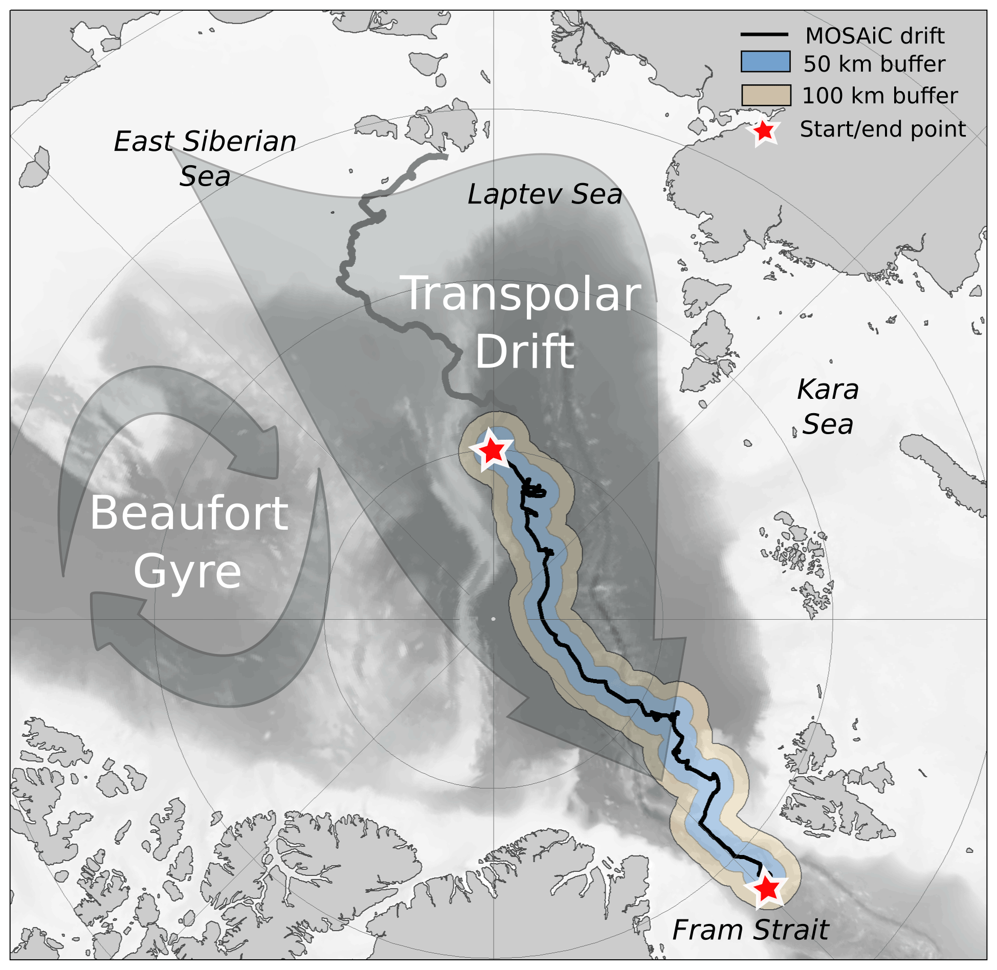
Figure 1 The MOSAiC drift (black line; the Central Observatory, CO) with a 50 km (blue) and 100 km (orange) buffer. The start (4 October 2019) and end points (31 July 2020) of the first MOSAiC expedition phase are indicated by red stars. Following Krumpen et al. (2020), the MOSAiC floe originated from the New Siberian Islands (thick gray line). The bathymetry of the Arctic Ocean (gray shading in the background) is based on Jakobsson et al. (2012).

Ice conditions found on site at the start of the drift experiment were exceptional to begin with. Record temperatures in summer and strong offshore-directed ice drift in winter resulted in the second longest ice-free summer period since reliable instrumental records began. As a result, ice thickness was unusually thin compared to the previous 26 years (Krumpen et al., 2020). However, by the time the MOSAiC floe reached the Fram Strait (around 300 d later), it had grown to a thickness typical for the region in summer in the past decade (results from IceBird airborne surveys; Fig. 1 in Belter et al., 2021).

Satellite data played a decisive role in the campaign. Using a combination of satellite images acquired prior to the start, Krumpen et al. (2020) were able to follow the ice floe back to its place of origin, namely the shallow shelf of the New Siberian Islands (Fig. 1). During the drift itself, satellite images were continuously taken over the ship and the extended surroundings to support scientific objectives and logistic needs. Especially during the polar nights, these data became the only systematic source of information about the ice conditions in the wider area. In this paper, we make use of satellite data records collected along the drift track to categorize the different ice conditions and most prominent events that shaped and characterized the floe and surroundings from 4 October 2019 to 31 July 2020. A comparison with previous years is made whenever possible for the reference period 2005–2006 to 2018–2019. The reference period was chosen such that it includes as many data products as possible. The aim of this analysis is to provide a very first and general overview of on-site conditions for upcoming physical, biogeochemical and ecological MOSAiC studies.

Below, we introduce the different satellite products used to describe the sea ice conditions along the drift. A short description of the large-scale atmospheric pattern and its impact on the Transpolar Drift is provided. A more detailed description of the atmospheric conditions is given in Dethloff et al. (2021) and Rinke et al. (2021). Hereafter, we analyse the drift itself and reconstruct the course that the ship would have taken in previous years. This is followed by an analysis of ice concentration, ice thickness, snow thickness and deformation and lead openings along the drift. Finally, we take a first glimpse at the distribution of melt ponds on the MOSAiC floe using high-resolution Sentinel-2 data collected before the CO entered the Fram Strait and started to disintegrate. At the end of each section, key research questions are identified that should be addressed in future studies. In closing, we summarize the main findings.

2 Material and methods

The Transpolar Drift carried Polarstern with the MOSAiC CO from its initial position on 4 October 2019 (85^∘ N, 136^∘ E) to the Fram Strait (31 July 2020, 78.9^∘ N, 2^∘ E) within 303 d. Hereafter, the ship was relocated to a position near the North Pole (87.7^∘ N, 104^∘ E on 21 August 2020), an area with limited satellite coverage. In this paper, we, therefore, exclusively focus on the first phase of the MOSAiC expedition.

The 303 d long drift is reconstructed using GPS data from different sensors. From 4 October 2019 to 15 May 2020, we use the ship's GPS. Because Polarstern had to leave the CO temporarily from mid-May until 18 June for the purpose of crew exchange, this period was bridged with GPS data provided by a surface buoy deployed on the CO prior to departure (buoy ID P225; https://www.meereisportal.de/, last access: 22 June 2021). For the remaining period until 31 July, we again use the ship's GPS data. In the following, the data products utilized to describe the ice conditions in the vicinity of the MOSAiC floe are introduced. An overview of the different products and their spatial and temporal resolution is given in Table 1. Where possible, we compare data in the full resolution of the respective satellite with mean values formed over a 50 and 100 km radius (Fig. 1; buffer).

Table 1 List of parameters and products investigated along the MOSAiC trajectory, with their respective satellite platforms and data distributors, as well as their resolution (temporal and spatial), investigated radii and corresponding terminology.

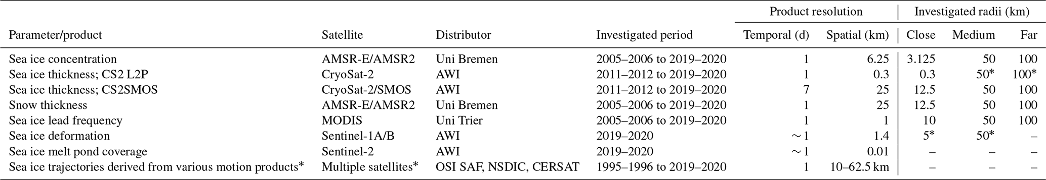
^* See Sect. 2 for details. AWI – Alfred Wegener Institute; OSI SAF – Ocean and Sea Ice Satellite Application Facility; NSDIC – National Snow and Ice Data Center; CERSAT – Centre d'Exploitation et de Recherche SATellitaire; AMSR-E – Advanced Microwave Scanning Radiometer for EOS; AMSR2 – Advanced Microwave Scanning Radiometer 2; SMOS – Soil Moisture and Ocean Salinity.

2.1 Lagrangian sea ice tracking

To investigate whether the 2019–2020 drift was comparable to previous years, we made use of satellite sea ice motion data to reconstruct the pathways the ship would have taken if the experiment had started in one of the previous 14 years (October 2005–2018) instead. The satellite-based sea ice pathways were determined with a drift analysis system called IceTrack. The system traces sea ice forward in time using a combination of satellite-derived, low-resolution drift products (Krumpen et al., 2019, 2020; Belter et al., 2021; Wilson et al., 2021). In summary, IceTrack uses a combination of the following three different ice drift products for the tracking of sea ice: (i) motion estimates based on a combination of scatterometer and radiometer data provided by the Centre for Satellite Exploitation and Research (CERSAT; Girard-Ardhuin and Ezraty, 2012; 62.5 × 62.5 km grid spacing), (ii) the OSI-405-c motion product from the Ocean and Sea Ice Satellite Application Facility (OSI SAF; Lavergne, 2016; Lavergne et al., 2010; 62.5 × 62.5 km grid spacing), and (iii) Polar Pathfinder Daily Motion Vectors (v.4) from the National Snow and Ice Data Center (NSIDC; Tschudi et al., 2020; 25 × 25 km grid spacing). The IceTrack algorithm first checks for the availability of CERSAT motion data, since CERSAT provides the most consistent time series of motion vectors starting from 1991 to present and has shown reliable performance (Rozman et al., 2011; Krumpen et al., 2013). During the summer months (June–July), when drift estimates from CERSAT are missing, motion information is bridged with the OSI SAF product (2012 to present). Prior to 2012, or if no valid OSI SAF motion vector is available within the search range, NSIDC data are applied. The reconstruction of “virtual” floes for these 14 years works as follows: sea ice at the starting position of the CO is traced forward in time on a daily basis starting on 4 October (1996 to 2019) until 31 July (303 d). Tracking is discontinued if sea ice concentration at a specific location along the trajectory drops below 50 %, which the algorithm defines as the position at which the ice melted. The applied sea ice concentration product is provided by CERSAT (Ezraty et al., 2007) on a 12.5 km grid and is based on 85 GHz Special Sensor Microwave/Imager (SSM/I) brightness temperatures, using the ARTIST Sea Ice (ASI) algorithm (Kaleschke et al., 2001).

To assess the accuracy of this Lagrangian tracking approach, Krumpen et al. (2019) reconstructed the pathways of 56 GPS buoys deployed between 2011 and 2016 in the central Arctic Ocean. The displacement between real and virtual tracks is approximately 36 × 20 km after 200 d and considered to be in an acceptable range. To assess the accuracy of IceTrack in 2019–2020, we reconstruct the drift of the CO and 23 additional DN buoys (Krumpen and Sokolov, 2020). A comparison of Fig. 2a with b shows that the reconstructed drift of the CO and other buoys is in close agreement with the observed drift. However, when the CO entered the Fram Strait (red box), the reconstructed track lags behind the real one. The study of Krumpen et al. (2019) indicates that the limited performance of IceTrack in the Fram Strait is likely the result of a general underestimation of drift speeds by low-resolution satellite products in this area. It becomes particularly evident when looking at the reconstructed drift of the additional 23 DN buoys deployed in the vicinity of the CO (Fig. 2c). Within the first 200 d, the reconstructed DN trajectories deviate only slightly from observed tracks (28 × 15 km after 200 d), but once the DN reaches the Fram Strait (south of 82.5^∘ N after 250 d), the distance between real and reconstructed pathways increases exponentially. The comparison of the CO drift with the drift of the previous 14 years is therefore limited to the first 250 d.

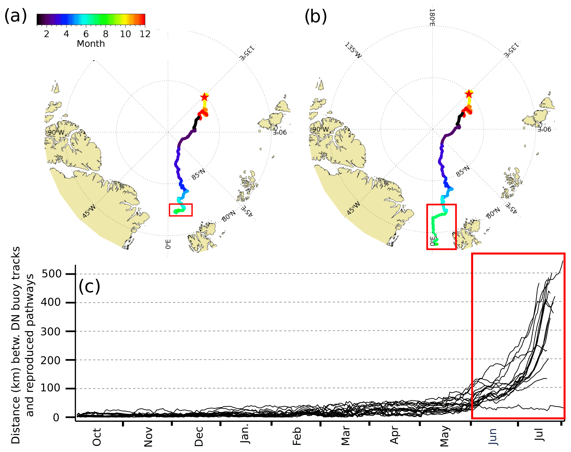
Figure 2 Comparison of MOSAiC CO and DN buoy tracks with IceTrack results. (a) Reproduced pathway of the CO with IceTrack. (b) Real (GPS-based) track of the CO. (c) Distance between 23 DN buoys (source: https://seaiceportal.de, last access: 18 August 2021) deployed on sea ice in the vicinity of the CO at the beginning of October2019 and their reconstructed trajectories. Deviation between real and virtual tracks is small. Only once buoys enter the Fram Strait (beginning of June (day 240) at 82.5^∘ N), does the distance gradually increase (red box).

2.2 Sea ice concentration

A time series of sea ice concentration along the MOSAiC trajectory between October to July (daily resolution) is obtained from the 89 GHz channels of the Advanced Microwave Scanning Radiometer for EOS (AMSR-E) and Advanced Microwave Scanning Radiometer 2 (AMSR2) on the NASA Aqua and the Japan Aerospace Exploration Agency (JAXA) Global Change Observation Mission – Water (GCOM-W) satellites, respectively (Table 1, Spreen et al., 2008; Melsheimer and Spreen, 2019a, b). Data are available from https://meereisportal.de and https://seaice.uni-bremen.de (last access: 15 February 2021). The spatial resolution of the data set is 6.25 km grid spacing (the footprint sizes of the two sensors are, with 4 and 5 km, even smaller). The conditions in larger surroundings are determined by averaging all grid points falling within a 50 and 100 km radius (compare Table 1). For comparison with previous years, we extracted sea ice concentration along the MOSAiC trajectory for the years 2005–2006 to 2019–2020. The year 2011–2012 is left out due to a gap between AMSR-E and AMSR2. Uncertainties (accuracy and precision) are usually below 5 % for individual grid cells in winter and in the high ice concentration regime. In summer and at low ice concentration, uncertainties can be significantly larger (up to 25 %; Spreen et al., 2008). Also, atmospheric influences like cloud liquid water and water vapour can affect the sea ice concentration retrieved from 89 GHz channels. However, these are uncertainties of individual grid cells and mean biases for the averaged 50 and 100 km radii are lower if they are not affected by larger-scale phenomena or summer melt. In summer or during warm air intrusions, sea ice concentration underestimation due to wetted ice surfaces, ice lenses or higher liquid water content in the snow or melt ponds might occur. Such a period is observed during MOSAiC from mid-April to May 2020 and discussed below. During that time period, we show, for comparison, sea ice concentration from an inverse multiparameter retrieval based on AMSR2 data using optimal estimation (Scarlat et al., 2017, 2020). It uses all frequency channels from 7 to 89 GHz to retrieve seven surface and atmospheric parameters (including cloud liquid water and water vapour), which can potentially mitigate some of the effects, like atmospheric influence causing wrong sea ice concentrations for traditional single-parameter satellite retrievals like the one introduced above. The spatial resolution of this data set is approximately 40 km. During and following the warm air intrusion and the associated drizzle-on-snow event, it shows more correct ice concentrations but is yet not available for the previous years and, thus, cannot be used as a primary data set here.

Based on the 89 GHz sea ice concentration data set, we also calculate the closest distance from the MOSAiC CO to the ice edge. To remove small openings in the ice, we first smooth the sea ice concentration data set by convolution with a 4×4 (25 km) grid cell kernel; then the distances from the CO grid cell to all grid cells with zero sea ice concentration are calculated, and the shortest distance is selected as distance to the ice edge.

2.3 Sea ice thickness

Sea ice thickness (SIT) along the MOSAiC drift track during the Arctic winter season from October 2019 through April 2020 is analysed using two satellite remote sensing data sets. The first data set is based on radar altimeter data from the CryoSat-2 (CS2) mission of the European Space Agency (ESA). We use SIT retrievals generated at the full resolution of the altimeter with an approximate point spacing of 300 m and swath width of 1650 m along the ground track of the satellite (Table 1). The method of the SIT retrieval for each radar waveform is based on Ricker et al. (2014), with updates described in Hendricks and Ricker (2020). The data set is named the Alfred Wegener Institute (AWI) CryoSat-2 sea ice thickness product version 2.3, and it is accessible through the website https://meereisportal.de (last access: 15 February 2021). In this study, we use the level 2 pre-processed (L2P) product between 1 October 2019 and 30 April 2020. This processing level contains data from CryoSat-2 radar echoes along the ground tracks of all orbits within 1 d, and SIT information is provided for each radar footprint of approximately 300 m × 1600 m in the along- and across-track direction respectively. Spatial averaging is necessary to reduce the significant retrieval noise for the individual radar echoes but is not applied to the L2P data. Instead, subsets of all orbit data points within 1 d are generated based on their distance to the noon (universal coordinated time – UTC) position of the CO. For each subset, we compute the mean SIT, the interquartile (IQR) and interdecile (ICR) SIT range, as well as the number of data points in each daily subset. According to the study logic, the search radius for the SIT subsets is chosen as 50 and 100 km, and we only use individual orbits that provide at least 50 data points within the specified search radii. Both the number of L2P data points per day and their minimum distance to the Polarstern noon position are variable. The number of CS2 L2P data points for the 50 km (100 km) search radii varies from approximately 50 (300) at lower latitude to approximately 900 (2000) close to the maximum orbit coverage of CS2 at 88^∘ N. No data within a short period in February 2020 are found at the 50 km search radius when the centre position of the search radius was above 88^∘ N, while the 100 km search radius is sufficiently large to match CS2 orbits. We do not show data from a smaller (e.g. 5 km) search radius, as very few orbits were close enough to the CO. For the same reason we also refrain from comparing short segments of L2P data to local observations on the CO, not only because of the lower temporal coverage but also because the retrieval noise in the L2P SIT data will dominate on the scale of the local SIT observations.

The second data set used for the SIT estimation is the merged CryoSat-2 and Soil Moisture and Ocean Salinity (SMOS; collectively CS2SMOS, version 203) SIT product (Ricker et al., 2017). CS2SMOS provides gridded SIT data at a resolution of 25 km, which is significantly lower than the CS2 L2P data; however, the underlying optimal interpolation provides gapless SIT information, also north of the CS2 orbit limit of 88^∘ N. CS2SMOS SIT estimates at the CO position during the short period when Polarstern drifted north of 88^∘ N are thus based on a spatial extension of SIT gradients measured at the CS2 orbit limit. Each daily updated CS2SMOS SIT field is based on an observation period of 7 d, and we use the centre of this period as the reference time to subset SIT data around the CO position at the selected radii. CS2SMOS data are based on CS2 L2P and SMOS SIT data. The SMOS retrieval provides thickness information of thin sea ice, which complements the CS2 L2P data. The data merging use a background field extending 2 weeks before and after the observation period; thus, the temporal coverage is shorter than that of the CS2 L2P data and ranges from 18 October 2019 to 12 April 2020. In addition, the selection of SIT observations in the CS2SMOS data may vary from the CS2 L2P regional coverage as we use the grid cell centre positions within 50 and 100 km radius around the CO to compute the daily mean CS2SMOS SIT value. The number of selected CS2SMOS SIT observations depends on the position of the CO relative to local grid cell coordinates. The number varies between 10 and 14 grid cells for the 50 km and between 47 and 52 for the 100 km search radius. We do not expect this variability to cause a selection bias due to the smoothness of the CS2SMOS SIT data.

2.4 Snow depth

Low-resolution snow depth along the MOSAiC trajectory is retrieved from the 7 and 19 GHz channels of the AMSR-E and AMSR2 microwave radiometer, following the method from Rostosky et al. (2018). Data are available via Rostosky et al. (2019a, b). Following Rostosky et al. (2020), uncertainties are based on Monte Carlo simulations using varying input parameters for a snow and sea ice (Microwave Emission Model of Layered Snowpacks – MEMLS; Tonboe et al., 2006) and atmosphere (Passive and Active Microwave radiative TRAnsfer – PAMTRA; Mech et al., 2020) microwave emission model. Most sea ice, snow and atmosphere properties are not known to the satellite snow depth retrieval (only information about the ice type, multi-year or first-year is provided; based on Ye et al., 2016a, b). Thus, by varying these properties and evaluating the influence on the snow depth retrieval, an estimate of the uncertainty caused by their unknown state can be obtained. The uncertainty range for snow depth on multi-year ice is between 5 to 10 cm on average (for individual grid cells it can be larger). The mean uncertainty estimate specifically for the MOSAiC data set is 8 cm. The grid size of the snow depth data is 25 km. The snow depth retrieval for multi-year ice areas is currently limited to March and April, while for first-year ice it can be retrieved all winter (see Rostosky et al., 2018). As the MOSAiC ice floe was in an area of predominantly second-year ice, which radiometrically is considered multi-year ice for the snow depth retrieval, snow depth for MOSAiC is only available for March and April. Here we present snow depth data for the grid cell centred at the CO (12.5 km radius) in addition to radii of 50 and 100 km averages (compare Table 1). A comparison with previous years is made with snow depth data extracted along the MOSAiC drift path from 2005 until 2019.

2.5 Lead detection based on optical data

Sea ice leads, i.e. lead frequencies and lead fractions along the MOSAiC drift track, are derived from Moderate-Resolution Imaging Spectroradiometer (MODIS) thermal infrared data and Collection 6 (C6) of ice surface temperatures (Hall and Riggs, 2019). In order to detect whether a lead is present in a certain pixel, we employ the local surface temperature anomaly, which is expected to exhibit significant positive deviations when a lead is present during winter (November to April). This general procedure is followed by the application of a fuzzy inference system that assigns individual retrieval uncertainties to each detected lead pixel. Using this approach, we obtain daily categorical lead maps with separate classes for clouds, sea ice, leads and artefacts, with the latter comprising detected leads with an uncertainty exceeding 30 %. The full approach and the resulting products are described in Reiser et al. (2020). From this data set, we use daily lead data with a spatial resolution of 1 km for the months of November to April for the years of 2005–2006 to 2018–2019 (as the reference period) and for the winter of 2019–2020 (for MOSAiC, compare Table 1). The daily lead data can only be derived for winter months as the retrieval relies on a significant surface temperature contrast between leads and sea ice. The derived lead frequency is a temporally integrated quantity that indicates how often a lead is found at a certain position within a defined period, while the lead fraction is a spatially integrated quantity that provides the fraction of an area that was covered by leads. Note that days with a cloud fraction above 50 % are excluded from the analysis.

2.6 Sea ice deformation from high-resolution radar images

In this study, we quantify sea ice deformation based on sequential Synthetic Aperture Radar (SAR) scenes obtained by ESA's Sentinel-1A/B satellites along the drift track of the CO. Deformation is the consequence of divergence (opening), convergence (closing) and shear (sliding alongside) between ice floes. Regularly gridded sea ice drift and deformation fields with a spatial resolution of 1.4 km are retrieved following the method described in von Albedyll et al. (2021). More details about the drift algorithm are provided in Thomas et al. (2008, 2011) and Hollands and Dierking (2011). As input for the applied algorithm, we use HH-polarized scenes with a spatial resolution of 50 m. Images over the CO were taken during the entire MOSAiC drift, except for the period between 14 January and 15 March 2020, when the ship was north of the satellite coverage. The temporal resolution is typically one image per day (with few exceptions). Spatial derivates are calculated from the gridded velocity field and used to derive divergence, convergence and shear (see von Albedyll et al., 2021 for details). To quantify deformation in the vicinity of the CO, we average all grid cells located within a 5 km radius around the ship. Exceptionally strong deformation events are defined as events with a magnitude exceeding 2 standard deviations of the 5 km average time series. To compare deformation in the vicinity of the ship with deformation over a larger area (50 km), averages are computed for 61 5 km circles arranged within a radius of 50 km around the ship (see illustration in Fig. 3). In this way, we avoid biases due to scaling effects.

Figure 3 To compare deformation in the vicinity of the ship (5 km) with deformation on larger scales (50 km), averages were computed for 61 5 km circles arranged within a radius of 50 km around the ship. Example of divergence, convergence (a) and shear (b) derived from two consecutive Sentinel-1 SAR images acquired on 14 April (07:26:14 UTC) and 15 (08:07:03 UTC) 2020. Sea ice motion is displayed as black arrows. The image pair shows the strongest deformation event observed. Within 24 h, a 2.5 km wide north–south-oriented lead opened up ∼ 25 km away from the CO.

2.7 Characterization of melt pond coverage using optical Sentinel-2 data

To provide a first quantification of the spatial distribution and temporal development of large melt ponds on the MOSAiC floe, we downloaded all available Sentinel-2 (S2, ESA) satellite images (https://scihub.copernicus.eu/dhus/, last access: 10 February 2021) taken over the ship between the end of May and 31 July 2020. Prior to the end of May, the Sun elevation was not high enough for passive optical remote sensing. A total of eight completely or partially cloud-free scenes could be identified. For the detection of melt ponds, we selected five scenes that are temporally equally spaced, namely 21 June, 1 July, 7 July, 22 July and 27  July 2020. Next, the MOSAiC floe was clipped, and a pond index was calculated by means of a normalized spectral index (e.g. Gignac et al., 2017; Watson et al., 2018) using S2 bands 4 (665 nm) and 8 (842 nm) as input. The pond index is used to differentiate between water and ice/snow. Note that only ponds larger than the spatial resolution of the S2 sensor (10 m) can be detected. We, therefore, assume that the actual pond cover is significantly underestimated, and that the method is only suitable for providing estimates of the timing and relative changes in pond coverage.

2.8 Reanalysis and ship weather data

Mean sea level pressure, 2 m air temperature and 10 m wind speed data for the time period 2005–2020 are taken from the newest version of the European Centre for Medium-Range Weather Forecasts (ECMWF) global reanalysis, ERA5 (Hersbach et al., 2020). Hourly values along the MOSAiC trajectory in 2019–2020 and in the preceding 14 years along the same trajectory are extracted by linear interpolation in time and space after triangulation of the rectangular 0.25^∘ ERA5 grid. The 2019–2020 trajectory data are evaluated against corresponding standard meteorological observations on board the Polarstern (https://www.awi.de/nc/en/science/long-term-observations/atmosphere/polarstern.html, last access: 22 February 2021). The ship measurements are, however, taken at non-standard heights (wind – 39 m; air temperature – 29 m; pressure – 16 m, reduced to sea level) so the evaluation is rather qualitative. More stringent comparisons of MOSAiC in situ meteorological observations, not just from the ship but from a large number of sensors across the CO and DN, are beyond the scope of this paper but will be conducted elsewhere.

3 Results and discussion

3.1 Atmospheric conditions and the Transpolar Drift in 2019–2020

Large-scale surface air pressure and associated anomalies in 10 m wind speed (shown in Fig. 4) determined the course of the MOSAiC drift and its deviation from the long-term average. October, November and December were characterized by moderate monthly mean circulation anomalies, oriented mostly such that the winds (and thus the drift) were westward rather than northward, thereby preventing the MOSAiC floe from reaching the North Pole (note that Fig. 4 shows wind anomalies, whereas the drift path is the actual drift). Starting in January, large-scale low pressure entered the Arctic from the European sector, resulting in an intensification of the Transpolar Drift in January, February and March (Fig. 5), with the low-pressure region gradually moving towards the Beaufort Sea. Correspondingly, these months were associated with an exceptionally high positive Arctic Oscillation (AO) index (see Dethloff et al., 2021, and Rinke et al., 2021, for a more detailed description). In April, the decaying low-pressure centre was located over the Beaufort Sea, resulting in a drift of the MOSAiC floe towards the Barents Sea. Next, the reversed air pressure gradient in May, with a high-pressure anomaly over the Beaufort Sea, pushed the MOSAiC floe towards northeastern Greenland until it entered the Fram Strait area (June–July).

Figure 4 Monthly mean sea level air pressure (shading) and 10 m wind (arrows) anomalies with respect to the reference period of 2005–2019 for each month of the MOSAiC drift from October 2019 to July 2020. The complete drift path is denoted by cyan lines; the drift during the respective month is denoted by blue arrows.

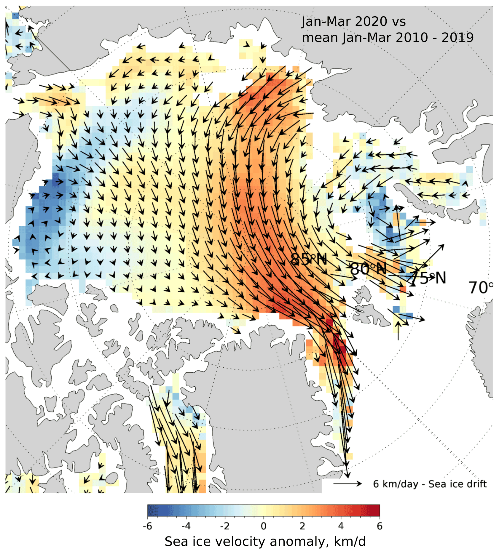
Figure 5 The 3-month (January–March) sea ice velocity anomalies in 2020 with respect to the reference period 2010–2019. Anomalies were computed from the OSI-405-c motion product provided by the Ocean and Sea Ice Satellite Application Facility (OSI SAF; Lavergne, 2016). The vectors plotted on top indicate the average daily sea ice motion for the same period (reprinted from Dethloff et al., 2021).

Figure 6 compares ERA5-based atmospheric conditions along the MOSAiC drift trajectory with conditions in the preceding 14 years. The circulation anomalies from January through May (Fig. 4) led to positive air temperature anomalies in northern Siberia and in the Kara and Laptev seas, in particular in February (up to +10 K; not shown). In contrast, air temperature anomalies at the MOSAiC floe were rather moderate most of the time (Fig. 6; middle). Moderate warmer-than-average periods occurred in mid-November, late February, mid-April and late May, whereas colder-than-average periods occurred in early November and early March, with absolute minima around −35 ^∘C. Wintertime cold (warm) anomalies were typically associated with high (low) surface air pressure anomalies (Fig. 6; bottom). The positive AO months of January, February, March and April were accompanied by low-pressure anomalies at the MOSAiC floe (Fig. 6 bottom). High wind speeds were encountered in particular in these months but also in late November and early December (Fig. 6 top). Apart from these exceptions, meteorological conditions at the MOSAiC floe can be considered average compared to previous years.

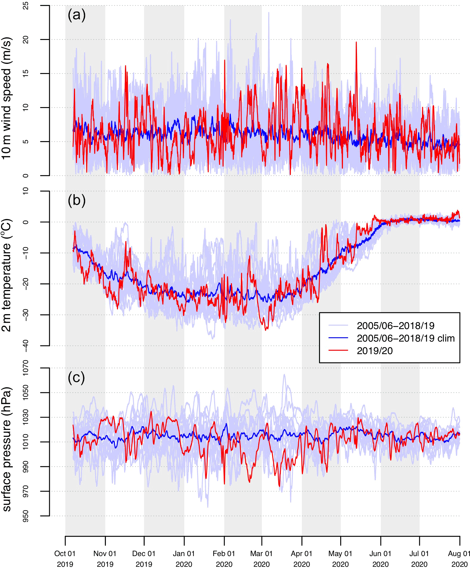
Figure 6 Hourly atmospheric conditions along the MOSAiC drift trajectory according to ERA5 in 2019–2020 (red) and in the preceding 14 years (light blue; average in dark blue). Panels show the (a) 10 m wind speed, (b) 2 m air temperature and (c) surface air pressure, respectively. See Fig. 7 for a comparison with corresponding ship observations.

The ERA5 data along the MOSAiC trajectory in 2019–2020 agree well with co-located ship observations (Fig. 7), in particular regarding surface air pressure. Wind speed tends to be slightly lower in ERA5, although it should be noted that the comparison with the raw on-board observations (e.g. winds are measured at 39 m instead of 10 m) has limitations. However, the winter warm bias in ERA5 over Arctic sea ice of the order of 2–3 K (Fig. 7) is consistent with previous assessments (e.g. Batrak and Müller, 2019). Note that the true 2 m air temperature bias might be even larger because the ship air temperatures might be overestimated due to (i) local heat sources and (ii) higher temperatures at the measurement height of 29 m compared to 2 m in typical cases of near-surface inversion. Given that these differences are likely systematic and, thus, similar in other years, the anomalies discussed above are likely not strongly affected.

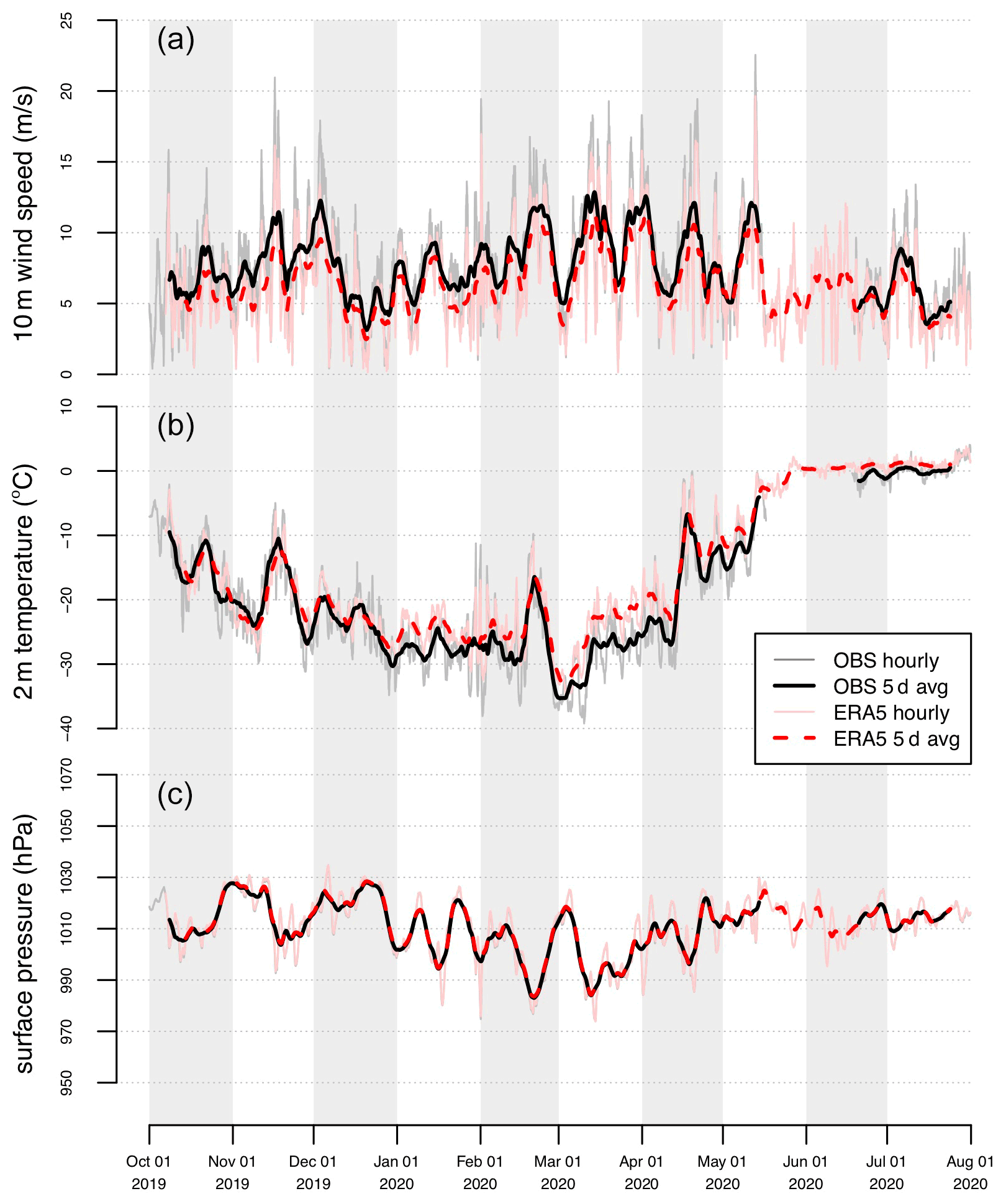
Figure 7 Atmospheric conditions along the MOSAiC drift trajectory in 2019–2020 according to ERA5 (red and light red) and according to ship measurements (black and gray). Hourly data are depicted in light red and gray; the 5 d averages are depicted in red (dashed) and black. Panels show the (a) 10 m wind speed, (b) 2 m air temperature and (c) surface air pressure, respectively.

3.2 The MOSAiC drift and a comparison to previous years

We compared the drift of the MOSAiC floe with the course the CO would have taken if the experiment had started in any of the previous 14 years (October 2005–2018). The underlying satellite-based Lagrangian tracking approach is introduced in Sect. 2.1. Figure 8 summarizes the results of this analysis. Figure 8a shows the reproduced MOSAiC trajectory (multicoloured line) together with trajectories from previous years (gray lines). The large differences between the tracks show how difficult it is to accurately predict the course of a drifting platform and how large the spread of possible endpoints can be. Figure 8b provides the averaged satellite-derived daily displacement rates of the MOSAiC CO during the first 250 d as compared to the previous 14 years. With 8.52 km/d, the drift speed in 2019–2020 is around 20 % higher than the mean over the period from 2005 to 2018 (7.14 km/d × 0.75). Only 2008–2009 shows an even higher average displacement rate (8.79 km/d), although the Fram Strait is reached a few days later due to a more northerly route. Another striking year is 2018–2019, with only average daily displacement rates but a strong westward drift component, which would have carried the ship even faster toward Fram Strait than in 2019–2020. A trend towards a faster Transpolar Drift, as reported by Spreen et al. (2011) or Krumpen et al. (2019), cannot be deduced from this rather simple and spatially limited analysis. However, results shown here are in line with these studies.

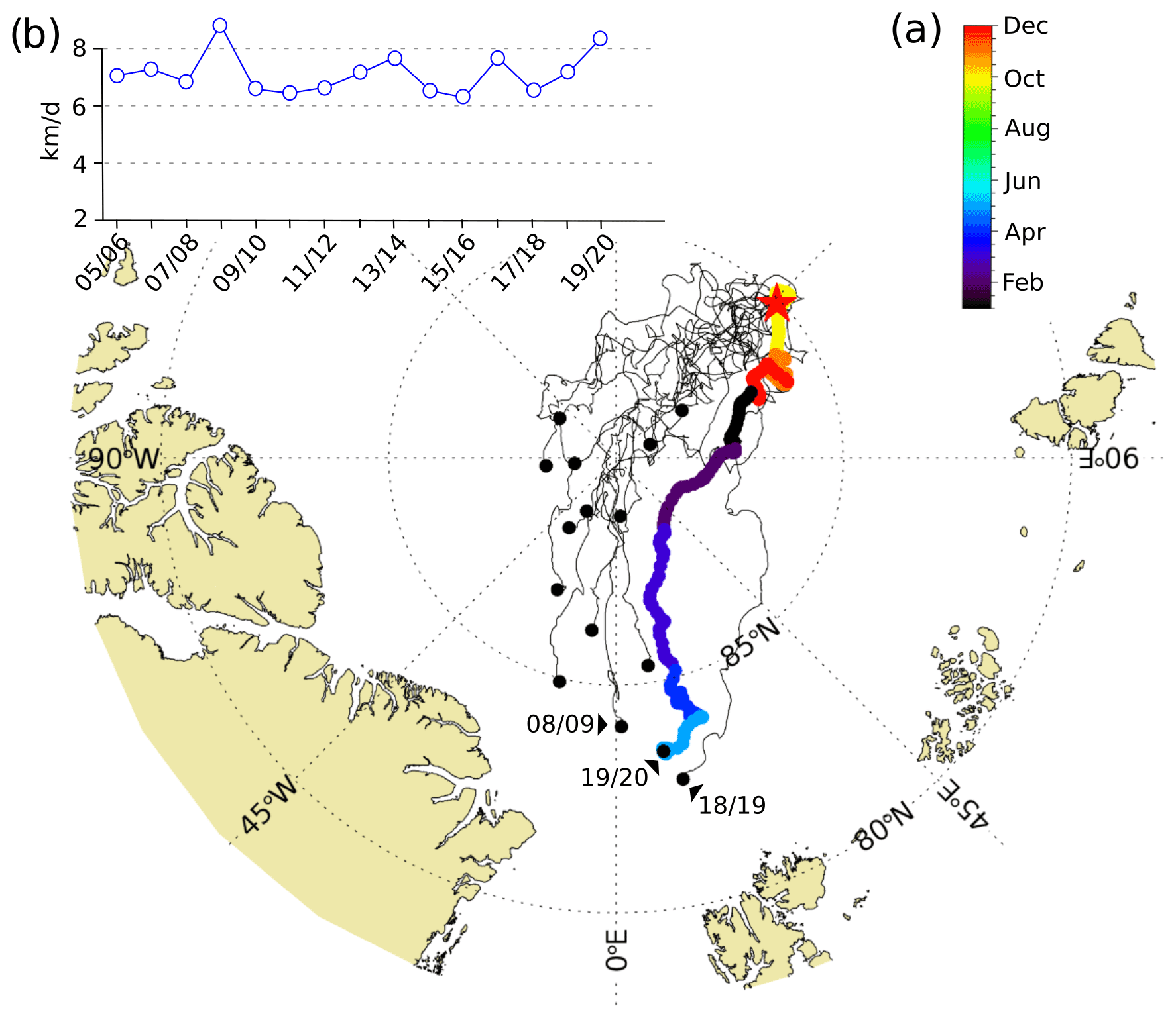
Figure 8 A comparison of the MOSAiC drift with the drift of previous years. (a) Results from a forward-tracking experiment. Sea ice was traced 14 times in a forward direction for a period of 250 d, starting on 4 October (2005–2019) from the position where the Polarstern drift started (red star). The multicoloured trajectory line, with colours corresponding to the month of year, indicates the reproduced drift of the MOSAiC CO (Central Observatory). All other years (2005–2018) are shown as black lines. The end nodes of the individual tracks are marked by a black circle. (b) Averaged displacement of sea ice per day (kilometres) for individual years.

3.3 Sea ice concentration

Sea ice concentration along the MOSAiC drift trajectory in 2019–2020 and the reference period (2005–2006 to 2018–2019) is shown in Fig. 9. The average sea ice concentration between 4 October 2019 and 31 July 2020 amounts to 97 % (based on the 89 GHz sea ice concentration – shown with the black line – i.e. containing the underestimation in April discussed below; Spreen et al., 2008). The seasonal evolution is characterized by a substantial temporal variability over the course of the 303 d long drift. This variability is almost independent of the spatial scale used with only minor differences (±0.5 % deviation from mean) between the sea ice concentration values determined from the 3, 50 and 100 km radius (Fig. 10).

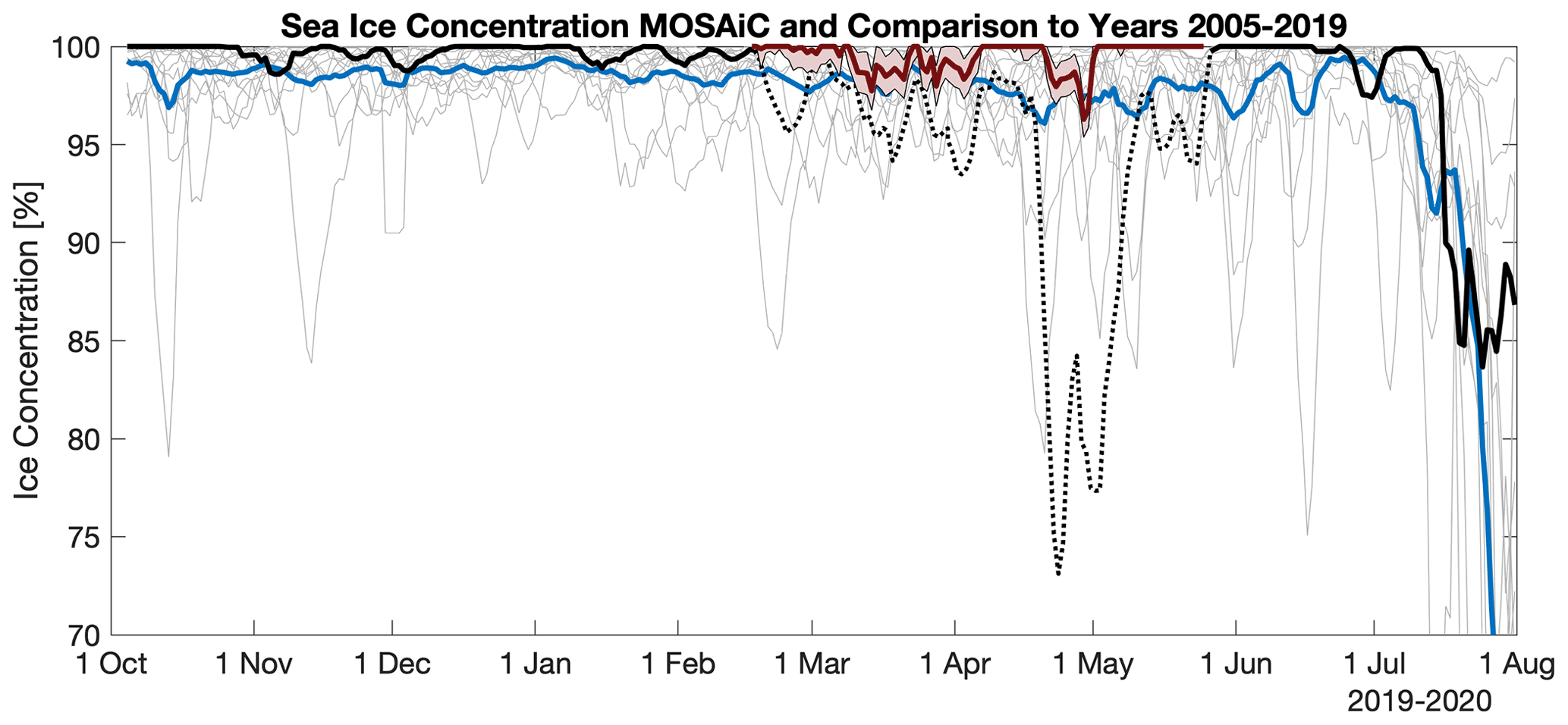
Figure 9 Sea ice concentration within a 3 km radius around the CO (6.25 km grid cell; black) along the MOSAiC drift from 4 October 2019 to 31 July 2020 in comparison to the ice concentrations from 2005–2006 to 2018–2019 for the same drift trajectory. The blue line shows the average for 2005–2006 to 2018–2019, while the gray lines show the individual years. All time series are smoothed with a 5 d running mean. During spring, warm air intrusions caused a significant temporary reduction in the sea ice concentration (dashed black line). We, therefore, show that with uncertainty estimates, in addition to an alternative sea ice concentration data set during the time (red and shaded red; not available for the climatology; see main text).

Given the high agreement between the values from different radii, we focus, in the following discussion, on the time series with the highest resolution (3 km radius; Fig. 9). The October to July sea ice concentration average along the MOSAiC drift trajectory agrees well with the long-term 2005–2006 to 2019–2020 average (both have a mean of 97 %). However, on shorter timescales there are significant differences. During the first half of the drift (October until end of February) the MOSAiC ice concentration was, with 99.5 %, about 1 % higher than the long-term average (compare black line with blue; Fig. 9), while during the second half (March until end of July), it was lower than during the long-term average and showed higher variability than the first half. High ice concentration, like 99.5 %, is not unusual (compare to the gray lines) and can be expected in winter in the central Arctic (e.g. Kwok, 2002). The second half with lower (actually false) ice concentration is more unusual and will be discussed further in the following.

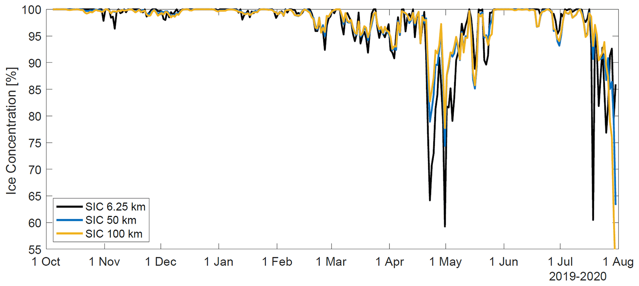
Figure 10 Sea ice concentration along the MOSAiC drift trajectory from the start of the drift on 4 October 2019 until the end of the first floe on 31 July 2020. Daily (no smoothing) sea ice concentrations are shown at 3.125 (black), 50 (blue) and 100 km (yellow) radii. Note the significantly underestimated concentrations between mid-April to May and the associated discussion in the main text and Fig. 9.

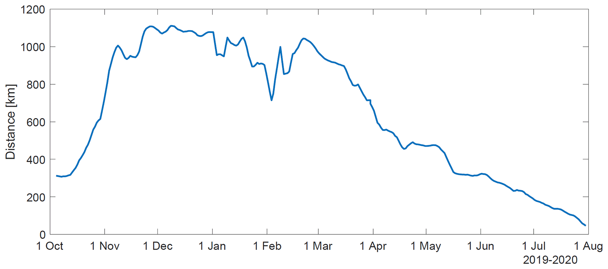
Figure 11 Distance of the MOSAiC CO to the ice edge obtained from the sea ice concentration data set.

Sea ice concentration variability stayed below 5 % until March 2020, when first significant reductions in ice concentration occurred. At this time, the CO was already positioned north of the Fram Strait, and the distance to the ice edge was gradually decreasing (compare Fig. 11). With the onset of spring in March–April, the first major drops in ice concentration below 90 % occurred. The strong ice concentration reductions down to 75 % from mid-April until mid-May (average ice concentration of 87 %) were due to a false satellite ice concentration retrieval. Visual observations from the ship's bridge confirm that the ice concentration, on average, stayed higher than 95 % during that time period. We can see that, at that time, a warm air intrusion raised temperatures close to 0 ^∘C, which was accompanied by a significant increase in wind speed (Fig. 6). The warming induced strong temperature gradients and increased vapour fluxes in the snow, which can cause stronger snow metamorphism and significantly change the snow permittivity already at above −5 ^∘C snow temperatures (Mätzler, 1987). Also, liquid water content can increase at temperatures slightly below 0 ^∘C, and small liquid water fractions of, e.g., 2 % strongly change the microwave loss in the snow (Hallikainen, 1986). Refreezing after the warming event can cause ice lenses in the snow. Such events were previously observed to have an influence on microwave properties and penetration (e.g. King et al., 2018). On April 2019, slight drizzle was observed, which likely refroze on the snow afterwards. These surface processes and additional weather influence by high water vapour and cloud liquid water affect the microwave polarization difference (e.g. Lu et al., 2018) and likely caused the strong fluctuation in ice concentration for the ASI algorithm used here. Other ice concentration algorithms for AMSR2 satellite data (e.g. NASA team) showed similar effects (not shown). As an alternative, we present the ice concentration from an optimal estimation retrieval (Scarlat et al., 2018, 2020) during that critical time period in Fig. 9, which attempts to take such effects into account (specifically the atmospheric influence), and in our case, it is in better agreement with the ship-based observations. Also, in previous years (gray lines; Fig. 9) occasionally ice concentrations below 90 % were observed in the sea ice concentration record during mid-winter. We have not investigated if these were real openings in the ice caused by ice divergence or atmosphere-induced effects like in our 2020 case. After mid-May 2020, the ice concentration recovered to almost 100 %. In July, the floe started to disintegrate and ice concentration dropped to 85 % within a radius of 3 km around Polarstern, and below 60 % in the 50 and 100 km radii (Fig. 10).

We determine the closest distance to the ice edge from sea ice concentration maps (Fig. 11). At the beginning of the MOSAiC expedition, the distance from the CO to the ice edge was about 320 km. During October, the distance gradually increased to 1000 km due to the freeze-up of the Russian marginal seas. Once the MOSAiC CO approached the Fram Strait (March 2020), the distance to the ice edge steadily decreased until the ice margin was reached at the end of July 2020. Note that the winter variability in ice edge distance was caused by polynya activity in the Russian shelf seas.

Future studies will investigate the impact of the warm air intrusion on microwave properties in more detail based on the extensive in situ microwave and snow/ice measurements conducted on the MOSAiC floe. However, the smaller fluctuations of the sea ice concentration between 97 % and 100 % during October to February need further investigation by combining them more closely with the different lead fraction and ice divergence records discussed below. This will help us to investigate the partitioning between thermodynamic and dynamic redistribution of ice mass, as well as the impact of ocean to atmosphere heat fluxes.

3.4 Sea ice thickness

Both satellite-based sea ice thickness products show the expected increase in ice thickness between October 2019 and April 2020 (Fig. 12 and Table 2). Except for the period between 14 February to 8 March 2020, when the CO was positioned north of 88^∘ N, the high orbit density of CS2 allows almost continuous daily coverage at 50 and 100 km radius. The monthly mean thickness within a 50 km (100 km) radius around the CO changed from 0.77 m (0.8 m) in October 2019 to 2.40 m (2.51 m) in April 2020. The sea ice thickness distribution is characterized by the IQR (difference between 75 % and 25 % percentile) and the interdecile range (IDR; difference between 90 % and 10 % percentile; compare Sect. 2. The increase in sea ice thickness was accompanied by a similarly increased IQR and IDR, indicating a wider sea ice thickness distribution as a result of thermodynamic ice growth and deformation of the older ice class and the formation of young ice throughout the winter season. Specific dynamic events sensed by other remote sensing sensors have a visible impact on the change of mean SIT and, thus, the apparent SIT growth rates. Lead formation in mid-November 2019, also seen in a strong divergence event, added new thin ice coincides with an intermittent SIT decrease (Fig. 19). The SIT distribution in the second half of April 2020 also widened significantly at a time when both lead fractions and a drop in sea ice concentration indicates the presence of new ice formation.

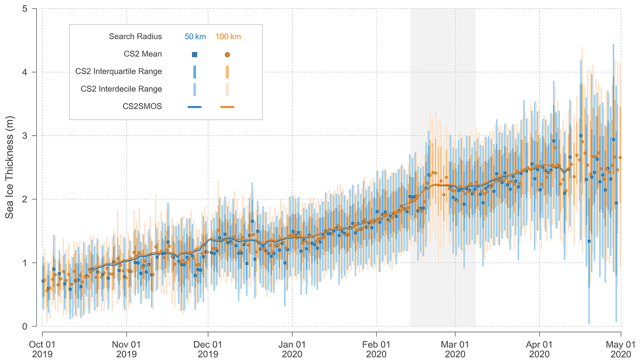
Figure 12 Daily sea ice thickness estimates from CryoSat-2 (CS2) full-resolution orbit L2P data and gridded CryoSat-2/SMOS (CS2SMOS) multi-sensor thickness analysis extracted for two different search radii (50 and 100 km) centred around the noon position of the CO for each day of the drift. Results from L2P data are only present for days where at least 50 L2P data points are found in both search radii. The gray rectangle indicates when the CO drifted north of 88^∘ N and outside the CS2 orbit coverage. The distribution of CS2 orbit data within the search radii is described by the mean value, interquartile (25 % to 75 % percentiles) and interdecile ranges (10 % to 90 % percentiles). For CS2SMOS, only the mean values of grid values within the search radius are provided.

Table 2 Monthly statistics of sea ice thickness (SIT) from CryoSat-2 (CS2) level 2P (L2P) orbit and gridded CryoSat-2/SMOS (CS2SMOS) data for two radii around the CO position. The CS2 SIT distribution is characterized by the interquartile range (IQR) as the difference between the 75 % and 25 % percentile and the interdecile range (IDR) as the difference between the 90 % and 10 % percentile. For CS2SMOS, the SIT difference (ΔSIT) between the MOSAiC year and SIT from the same drift trajectory, but of previous winters since 2010, is given. The asterisk (^*) indicates that the mean SIT of CS2SMOS depends on fewer years than the other month since the CS2SMOS data record only starts in November 2010.

It is also notable that the CS2 L2P sea ice thickness was, on average, consistently thinner at the 50 km radius compared to the 100 km radius (Table 2; on average 6 cm (4 %) thinner between October and April). Similarly, IQR and IDR were larger for 100 km than for 50 km; however, the larger number of data points in the wider search area may also lead to a higher likelihood of diverse sea ice conditions. This is in agreement with findings of Krumpen et al. (2020). According to the authors, the MOSAiC DN was set up at a regional thickness minimum. The local minimum is related to the ice age. Sea ice in the DN was formed 3 weeks later than the surrounding ice. However, Krumpen et al. (2020) report even larger differences in sea ice thickness of 36 % between the DN area and areas further away.

Results from CS2SMOS mirror these findings of thinner ice close to the CO compared to the larger scale, though differences are smaller (Fig. 12; Table 2). This can be expected, as the primary input to the CS2SMOS analysis in the central Arctic is CS2 data due to its higher sensitivity to thicker ice than SMOS. The main differences to CS2 L2P are therefore the influence of SMOS in the beginning of the winter and the larger degree of smoothing introduced by the optimal interpolation. The monthly mean sea ice thickness values in Table 2 are therefore mainly consistent, with the exception of October and November 2019. In this period, CS2SMOS was consistently higher by approximately 0.15 m with respect to the CS2 L2P data.

We do not expect that the locally lower thicknesses in the DN are well represented in the CS2SMOS SIT, since these are influenced by a larger region due to the interpolation method. The CS2 L2P thicknesses instead are effectively point measurements at kilometre scale and are apparently able to pick up the local thickness gradient with thickness differences smaller than the uncertainty of absolute SIT values. The discrepancy between the CS2 L2P and CS2SMOS thicknesses persisted well into November 2019 and became less prominent afterwards. This provides evidence that the local thickness minimum at the MOSAiC DN became less prominent over the winter season, though still at a detectable level as indicated by the consistent but minor differences at radii of 50 and 100 km.

Since CS2 L2P and CS2SMOS are in general consistent over the winter season, we use CS2SMOS data to compare sea ice conditions during the MOSAiC drift with the past nine winter seasons in the CS2SMOS data record (Fig. 13). The comparison between the years shows a comparably low sea ice thickness in the 10-year-long data record at the location of the MOSAiC expedition, if not the lowest for segments in the earlier part of the drift. The monthly sea ice thickness during MOSAiC was approximately 0.4 m lower at the beginning of the drift compared to mean monthly CS2SMOS of all previous winters (Table 2). The differences reduced towards 0.3 m in April, indicating slightly stronger thermodynamic and dynamic ice growth with respect to the average, potentially aided by the thinner sea ice at the beginning. These results are, however, based on a SIT data record that depends on climatological values for snow load and sea ice density and, thus, does not contain the impact by the expected variability in these parameters in the SIT retrieval. For example, using dynamic snow load in SIT retrieval by satellite radar altimeter has resulted in a more pronounced interannual variability but also stronger thickness trends in the Arctic marginal seas (Mallett et al., 2021). While MOSAiC has taken place in the central Arctic with generally thicker ice and snow, a similar impact can be expected as well. We therefore consider it unlikely that the differences between the SIT estimates along the MOSAiC drift tracks for the 10 years of CS2SMOS data can be explained by retrieval uncertainty alone. Field observations with longer time series are needed to evaluate the stability of SIT retrievals over decadal periods (e.g. Khvorostovsky et al., 2020), which are not available for the location of MOSAiC.

CS2SMOS also indicates sea ice thickness differences between the 50 km radius and the 100 km radius, showing that the MOSAiC expedition took place in a local sea ice thickness minimum. It should be noted that the SIT differences, specifically between the two search radii, were well below the uncertainty estimate of the retrieval for both CS2SMOS and CS2. Gridded CS2 data indicate a retrieval uncertainty, on average of 0.5 and 0.7 m, between October 2019 and April 2020 at a scale of 25 km and monthly periods (Hendricks and Ricker, 2020). The main driver of the uncertainty magnitude, however, is less retrieval noise but rather the uncertainty of auxiliary parameters such as snow load and sea ice density. The deviation between actual values of these parameters and their parameterizations in the satellite retrieval is likely to have larger correlation length scales. Thus, the satellite sensors might be able to sense local SIT differences, though the absolute SIT uncertainty remains substantial. The finding of consistently thinner ice for the 50 km search radius compared to the 100 km search radius throughout the drift might be seen as a demonstration of this point.

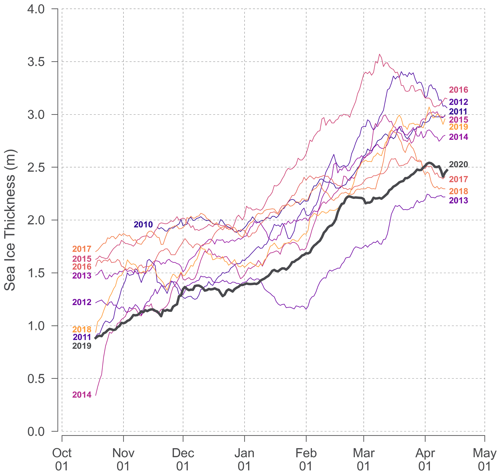
Figure 13 Daily sea ice thickness from gridded CryoSat-2/SMOS (CS2SMOS) multi-sensor thickness analysis extracted within 50 km of the CO noon position for all Arctic winters in the CS2SMOS data record. Each winter season is marked by the start and end year, e.g. 2011–2012. The bold black line indicates data during the MOSAiC year and is identical to the 50 km radius CS2SMOS data in Fig. 12.

Future work with the MOSAiC field data will focus on improving accuracy of SIT retrievals as well as quantifying its true magnitude. But given the sensitivity of present-day SIT products to local thickness differences and their sensitivity to dynamic events captured by other sensors, the question remains how SIT data at high spatial and temporal resolution can be used to better observe and understand the dynamics of the sea ice cover.

3.5 Snow depth

Figure 14 shows a time series of satellite-based snow thickness in March–April for the years between 2005 and 2020. The mean March–April snow depth during the MOSAiC year was 22 cm at the 12.5 km radius (22 or 23 cm in 50 or 100 km radius) with an uncertainty of 5 cm. Note that the observed snow thickness during MOSAiC is around 3 cm lower than the long-term average of the period 2005 to 2019. A preliminary comparison (not shown) of satellite-based snow thickness estimates with in situ observations from the MOSAiC CO indicates a good agreement with errors not exceeding the expected uncertainty of on average 5 cm.

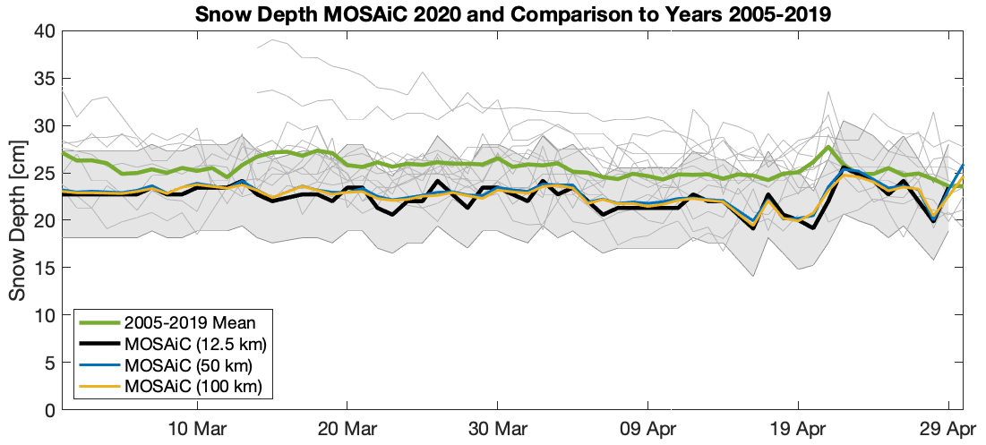
Figure 14 Snow depth from the AMSR-E and AMSR2 satellite microwave radiometers from 1 March to 30 April of the years 2005 to 2020 (without 2012) at the MOSAiC location. For the MOSAiC year 2020, the thick black line shows snow depth at 12.5 km radius. The gray shaded area indicates the corresponding uncertainty bounds (Rostosky et al., 2018, 2020). The blue and yellow line gives the mean snow depth at a 50 and 100 km radius for comparison. The thin gray lines show the individual years (2005 to 2019), and the green line provides the climatological mean. Because the MOSAiC floe was located in an area with partly second-year ice, snow depth can only be retrieved for March and April (Rostosky et al., 2018).

The snow depth during MOSAiC was a few centimetres lower but, overall, quite average compared to the long-term mean. The time series in Fig. 14 shows that the snow depth stayed almost constant from beginning of March until mid-April. Only after the warm air intrusion in April (Fig. 6), did increased precipitation lead to a small increase in snow depth of about 3 cm. This is in agreement but potentially a bit lower than the detected snowfall by several sensors in the MOSAiC CO (about 10–20 mm snow water equivalent, i.e. approx. 4–8 cm snow depth; Wagner et al., 2021). However, the Wagner et al. (2021) study also shows that snowfall does not always directly relate to snow depth increases because lateral snow redistribution plays a significant role. Future studies will evaluate the satellite snow depth in more detail based on the extensive snow measurements taken during MOSAiC.

The satellite AMSR-E/2 March–April 2020 snow depth of 22 cm is significantly lower than the snow climatology from Warren et al. (1999) for the years 1954 to 1991. For that depth, the March–April snow depth for the MOSAiC region would have been between 35 and 39 cm, i.e. 60 % to 80 % higher than during MOSAiC and the whole AMSR-E/2 time period from 2005 to 2019 (green line in Fig. 14). Thus, we observe a strong reduction in snow depth for the MOSAiC region compared to previous decades. This also has implications for ice thickness retrievals from satellite altimeters, where the Warren snow depth climatology often is used for the freeboard to ice thickness conversion (Sect. 2.3; e.g. Ricker et al., 2014).

Here we only present one satellite-based snow depth product. Future studies will compare our snow depth retrievals from the AMSR-E/2 microwave radiometers with snow depth from combined CryoSat-2 and ICESat-2 measurements (Kwok et al., 2020) and snow depth from SMOS (Maaß et al., 2013).

3.6 Leads

The mean winter lead frequency (November to April between 2005–2006 and 2018–2019) for the central Arctic Basin and adjacent seas is shown in Fig. 15a. The climatology shows that between November and April the central Arctic Ocean is generally characterized by low lead frequencies with values of roughly 0.1. This agrees well with consistently high ice concentration values indicated by the sea ice concentration climatology during the first half of the expedition (Fig. 9). According to the climatology, higher lead frequencies (> 0.15) in winter are only to be expected near the ice edge and in the Fram Strait. The lead frequency anomalies for the MOSAiC year 2019–2020 shown in Fig. 15b indicate no significant deviations from the winter mean climatology. On average, anomalies were slightly negative along the MOSAiC drift trajectory and in the sector between 30^∘ W and 120^∘ E, which again agrees well with the observed slightly higher ice concentration values as compared to the long-term mean (Fig. 9).

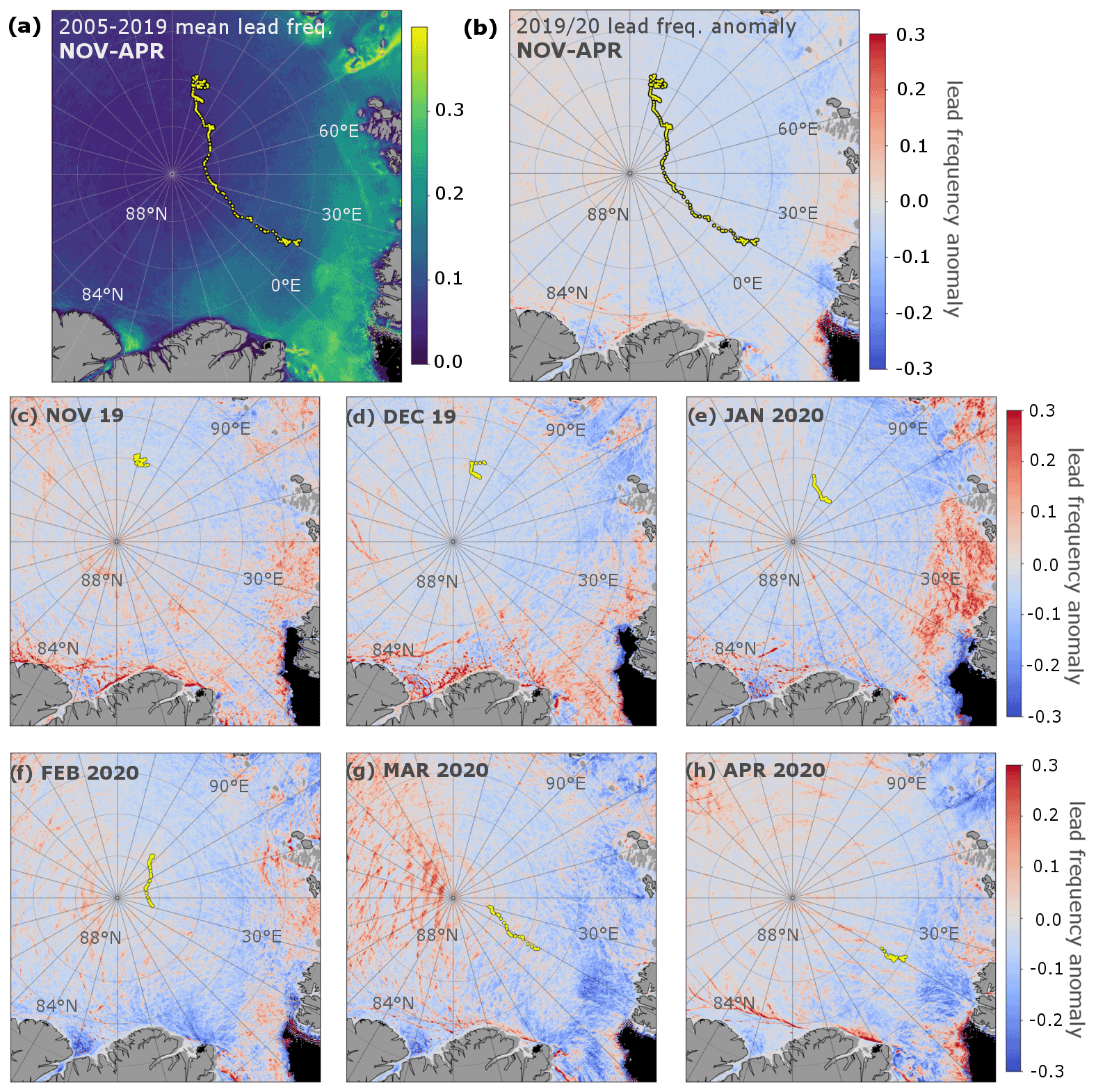
Figure 15 (a) Spatial distribution of the mean frequency of the occurrence of sea ice leads for the months of November to April for the winter seasons from 2005–2006 to 2018–2019 (reference period). MOSAiC drift of the CO is shown by yellow dots. (b) Lead frequency anomaly for the MOSAiC winter 2019–2020 with respect to the reference period. (c–h) Monthly lead frequency anomalies for the months of November to April in 2019–2020, respectively.

Regional differences in lead frequencies can be inferred from monthly lead anomaly maps shown in Fig. 15c–h. The monthly maps reveal anomalously high lead frequencies north of Greenland and Ellesmere Island between November 2019 and January 2020. Moreover, the strong positive anomalies in the Barents Sea in January 2020 and in the Beaufort Sea in February–March 2020 are worth mentioning (compare Dethloff et al., 2021). However, in the proximity of the CO no significant lead anomalies were found between November 2019 and February 2020. Only in March, when the CO was crossing a region of east–west-oriented leads, slightly higher anomaly values of up to 0.1 are indicated (compare Fig. 4). In April 2020, leads around the MOSAiC CO were more north–south oriented and strengthened as expressed by higher anomaly values of up to 0.2 (Fig. 15h).

A detailed view on the temporal evolution of lead fractions along the MOSAiC drift trajectory on different radii is presented in Fig. 16. However, meaningful conclusions can only be drawn for the periods in which the cloud fraction for the respective radii was below 50 %. Note that, in Fig. 16, days with missing data and higher cloud fractions are indicated by red dots. The lead fraction is shown for the area around the MOSAiC CO with 10, 50, and 100 km radius, together with the mean and maximum lead fraction for the reference period and 1 standard deviation. The mean lead fraction for the area around the CO was slightly increasing towards the end of winter for all of the three ranges shown, which confirms the drift into a region with generally higher average lead frequencies starting in March (Fig. 16a). In general, lead dynamics around the MOSAiC CO were typical for the respective region and point in time with only short, but significant, deviations from the mean. A maximum in lead activity was observed on 4 March (at all radii). Several smaller events with lead fractions exceeding 1 standard deviation from the reference period were recorded on 11–12 December, 19 January, 28 January, 1 February, 4–8 February, 1–5 March, 11 March and 23–24 April (for 50 km radius; Fig. 16a). Note that these events were only to some extent accompanied by a decrease in ice concentration, which might be explained by, e.g., differences in spatial resolutions and different thin-ice sensitivities of the respective sensors.

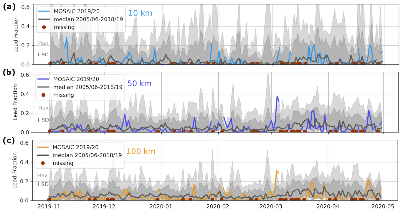
Figure 16 Temporal evolution of the lead fraction around the CO during MOSAiC for (a) a radius of 10 km (light blue), (b) 50 km (dark blue) and (c) 100 km (orange), respectively. Maximum (light gray area), mean (black line) and 1 standard deviation (dark gray area) of the lead fraction for the reference period 2005–2006 to 2018–2019 are shown for comparison.

3.7 Sea ice deformation

Figure 17 shows the time series of divergence, convergence and shear rates along the MOSAiC drift track at 5 and 50 km radii as obtained from Sentinel-1 SAR data. Overall, we find that deformation close to the ship (5 km radius) was representative for the deformation experienced by the ice cover at larger distances (up to 50 km). Despite the different geographical regions, we find that the mean shear and combined divergence and convergence of 8 % d⁻¹ and 2 % d⁻¹ along the MOSAiC drift track are in good agreement with deformation rates obtained from a ship radar north of Svalbard during the Norwegian young sea ICE (N-ICE2015) drift campaign (Oikkonen et al., 2017).

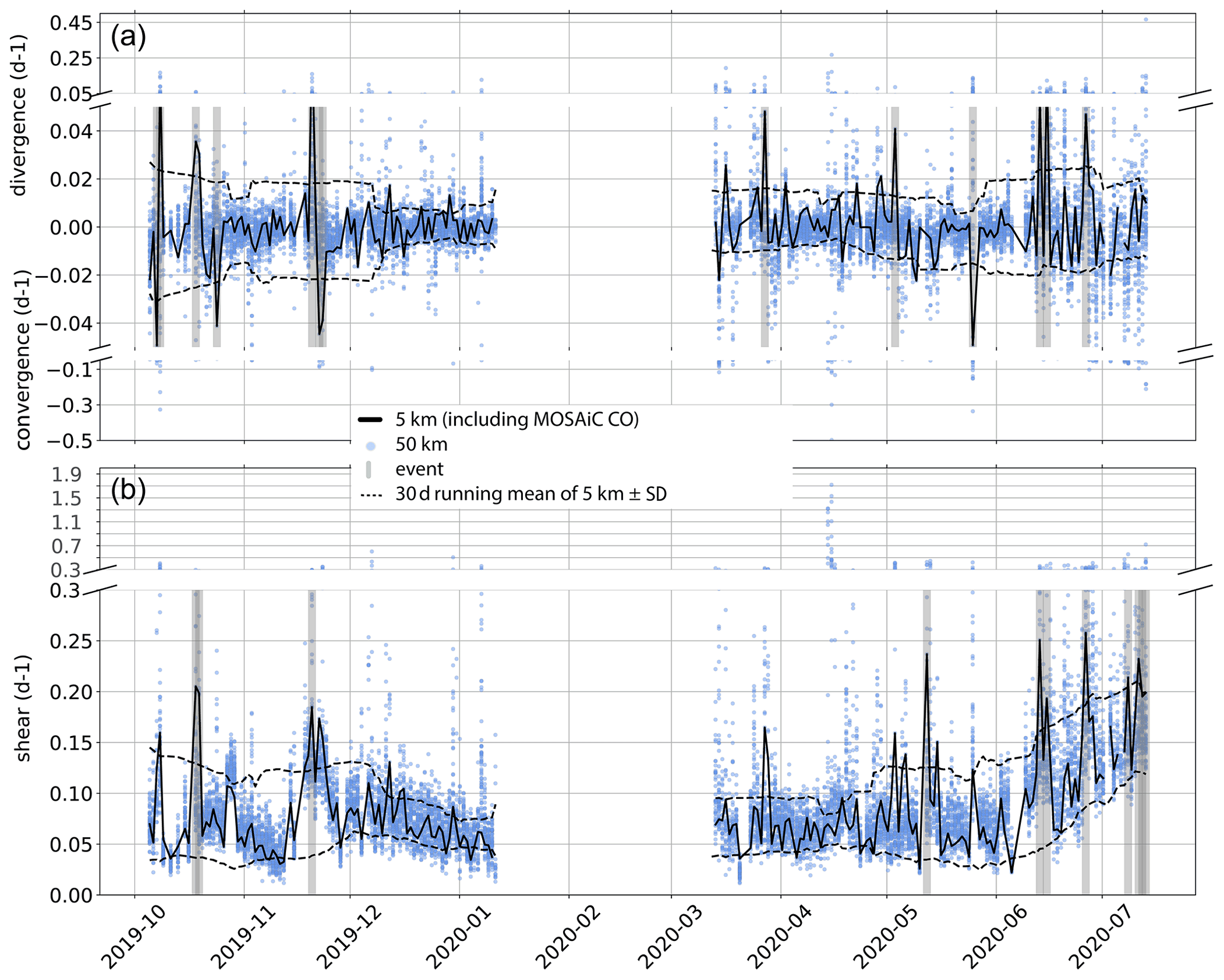
Figure 17 Time series of (a) divergence, convergence and (b) shear extracted from Sentinel-1 SAR scenes along the MOSAiC drift at different radii (5 km in black vs. 50 km in blue; compare Fig. 3) between 5 October 2019 and 14 July 2020. Strong deformation events with a magnitude of more than 2 standard deviations are marked by vertical gray bars. Successive events might overlap and look like one event. The 30 d running mean ± standard deviation illustrates the seasonal variability. Please note the change in the y axes' spacing to better display the larger deformation rates in spring and summer.

The variability in divergence, convergence and shear showed a seasonal behaviour which is linked to the consolidation of the ice pack and is in agreement with findings of previous studies (e.g. Itkin et al., 2017; Hutchings et al., 2011). Monthly averages of the time series indicate that deformation was moderate and balanced in convergence and divergence in the consolidation phase between October and November 2019 (Fig. 17). Hereafter, divergence, convergence and shear temporarily decreased from December 2019 to January 2020. In March to May 2020, divergence, convergence and shear went back to a moderate level until a sudden increase in June and July was observed when the MOSAiC CO approached the marginal ice zone. Note that monthly averaged divergence correlates reasonably well with intensified lead activity observed by optical satellites (Sect. 3.6). In spring (March and April), the ice experienced more divergent than convergent motion, which again agrees well with intensified lead activity observed in spring (Figs. 15 and 16).

On daily timescales, divergence, convergence and shear were characterized by long quiet phases occasionally interrupted by strong deformation events (see the video supplement). The average temporal spacing between such deformation events was 2.5 weeks. However, the events were not uniformly distributed in time, as 60 % of the events took place between October and November (gray bars in Fig. 17). The strongest deformation event within the 50 km radius of the CO was observed on 14–17 April 2020. By that time, a lead of almost 2.5 km width opened up at 25 km distance of the CO (Fig. 3).

We expect that future MOSAiC studies will investigate the driving processes behind seasonal and short-term deformation events in more detail, using a combination of on-ice, airborne and ship-based observations (e.g. stress measurements, airborne laser and thickness surveys and ship radar sequences) and data from various satellite products. We suggest the following future research questions: how does the ice thickness influence divergence, convergence and shear in response to the wind forcing, and what is the role of convergence in creating a thick ice cover and how does deformation shape the ice thickness distribution?

Figure 18 The top row shows the Sentinel-2 MSI true colour images of the MOSAiC floe obtained between 21 and 27 July 2020. The middle row shows an outline of the MOSAiC CO (black) and areas with classified melt ponds (pond index). The bottom row shows true colour images with the larger surrounding of the MOSAiC floe (black outline) and the temporal evolution of melt pond on the surface of neighbouring floes. The red star shows the position of Polarstern at the time of the satellite image acquisition.

3.8 Melt pond distribution

Figure 18 presents five cloud-free S2 scenes obtained between 21 June and 27 July 2020 that provide a first overview of the temporal and spatial evolution of melt ponds on the MOSAiC floe and its extended surroundings. Melt pond coverage is characterized using the pond index described in Sect. 2.7, where high values indicate water and low values indicate ice or snow.

One of the most striking features is that, at the time when the first cloud-free scene (21 July) was taken, large melt ponds had already developed on the MOSAiC floe. The earlier start of melt pond formation on the MOSAiC floe as compared to the extended surrounding is likely related to the surface topography. Compared to the surrounding floes, the MOSAiC floe was characterized by heavily deformed areas which may have favoured early accumulation of large meltwater ponds. Another possible reason for the early onset of melting may have been the high quantity of sediments that were trapped in the ice (Krumpen et al., 2020). The high sediment content temporarily reduced the surface albedo of the floe, which may have favoured the early melt of ice.

Within the following 10 days, the proportion of large melt ponds on the MOSAiC floe increased considerably, and large ponds also began to form on the neighbouring floes. On 7 July, while the total amount of melt ponds was still increasing, a few large melt ponds began to drain. In the final scene (27 July), taken almost 3 weeks after the draining began and just before the floe was abandoned, large melt ponds had mostly split into smaller ponds and had partially disappeared as a result of several drainage events that were observed in field between 1 and 27 July. The (absolute) quantification of melt pond fraction is limited, as the typical size of the melt ponds observed on the ground were equal to or smaller than the pixel size of the S2 image.

The unusual temporal and spatial evolution of melt ponds on the MOSAiC floe compared to the surrounding floes raises the question of what processes preconditioned the early melt. More specifically, what role did the heavily deformed area play in the formation of melt ponds, and to what extent did the presence of sediments accelerate melting processes?

4 Conclusions

Below we summarize the ice conditions along the drift of the MOSAiC floe and the extended surroundings and compare them to previous years (2005–2006 to 2018–2019). The analysis is based on satellite data products commonly used for the scientific analysis of sea ice in the Arctic Ocean. A summarizing overview of the atmospheric and sea ice conditions observed along track is given in Fig. 19.

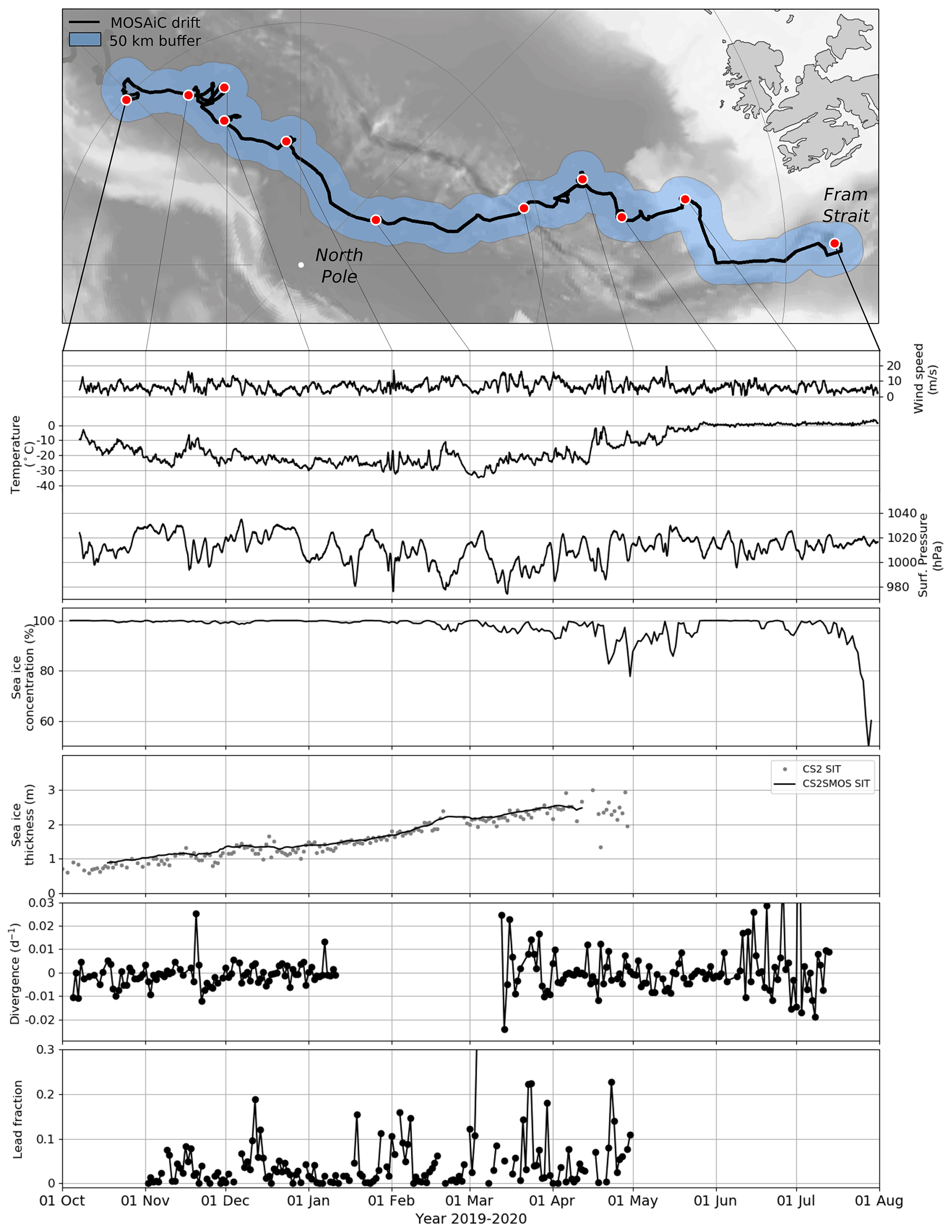
Figure 19 Summary of the atmospheric and ice conditions extracted from reanalysis and satellite data within a 50 km radius (top) along the MOSAiC CO drift track. Note that the drop in sea ice concentration in April–May is apparent only due to wet snow (see Sect. 3.3).

• A comparison of the MOSAiC trajectory with reconstructed satellite-based pathways for the past 14 years indicates that the drift during the first 250 d of the expedition was around 20 % faster than the climatological mean drift. Deviations from a long-term average drift path are, to a large extent, the consequence of prevailing large-scale low-air-pressure anomalies which resulted in an intensification of the Transpolar Drift between January and March 2020.

• CS2 and CS2SMOS data show that the mean thickness of sea ice around the CO (50 km radius) evolved from 0.77 m in October 2019 to 2.40 m in April 2020. Sea ice near the CO (50 km radius) was thereby 4 % thinner as compared to surrounding sea ice (100 km radius). According to Krumpen et al. (2020), the negative anomaly is due to the younger ice age, as the ice around the CO was formed in a different region and later in the year than the surrounding ice. A comparison with CS2SMOS records from the past nine winters shows that the ice around the MOSAiC CO was comparatively thin (partially the thinnest). In October 2019 it was 0.4 m, and in April 0.3 m it was below the 9-year average.

• Unlike ice thickness, snow thickness did not differ significantly from the long-term mean. Data from satellite-based microwave radiometers indicate an average March–April 2020 snow depth of 22 cm (12 km radius). This is 3 cm lower than the long-term mean for the years 2006 to 2019.

• From the start of the expedition until April, the average ice concentration within the 50 km radius of the CO was slightly higher (1 %) than the long-term mean, with low variability but occasional drops in ice concentration by up to 3 %, which would impact ocean–atmosphere fluxes. In April and May, a wrong reduction in sea ice concentration is observed in some sea ice concentration products as a result of a positive air temperature anomaly, which changed the microwave properties of the snow but did not melt it. A significant drop in ice concentration took place at the end of the first expedition phase when the floe approached the ice edge (July).

• An analysis of winter (October–April) lead frequencies inferred from MODIS thermal infrared data indicates no significant deviation in lead activity from the mean climatology (2005–2006 to 2018–2019). At most, a slight negative deviation from the winter mean is discernible, which agrees well with the positive anomaly in ice concentration between October and April. It is interesting to note that, with increasing variability in ice concentration from March onwards, lead activity increased.

• A deformation time series derived from Sentinel-1 data gives first insights into divergence, convergence and shear events along the MOSAiC drift path. Overall, we find that sea ice deformation on the 5 km radius, including the MOSAiC CO was representative for the wider (50 km radius) surroundings. Deformation rates were lower during winter and higher during summer, which is in agreement with observations from previous studies. The dominance of divergence during spring agrees well with the observed higher lead fractions.

• The five cloud-free S2 scenes obtained during the melting phase provide insight into temporal and spatial evolution of melt pond coverage on the MOSAiC floe. Particularly worth mentioning is that formation of melt ponds began earlier on the MOSAiC floe than on neighbouring floes.