the Creative Commons Attribution 4.0 License.
the Creative Commons Attribution 4.0 License.
 | 17 Aug 2021
Multiscale variations in Arctic sea ice motion and links to atmospheric and oceanic conditions
Dongyang Fu
Bei Liu
Yali Qi
Guo Yu
Haoen Huang
Lilian Qu
Arctic sea ice drift motion affects the global material balance, energy exchange and climate change and seriously affects the navigational safety of ships along certain channels. Due to the Arctic's special geographical location and harsh natural conditions, observations and broad understanding of the Arctic sea ice motion are very limited. In this study, sea ice motion data released by the National Snow and Ice Data Center (NSIDC) were used to analyze the climatological, spatial and temporal characteristics of the Arctic sea ice drift from 1979 to 2018 and to understand the multiscale variation characteristics of the three major Arctic sea ice drift patterns. The empirical orthogonal function (EOF) analysis method was used to extract the three main sea ice drift patterns, which are the anticyclonic sea ice drift circulation pattern on the scale of the Arctic basin, the average sea ice transport pattern from the Arctic Ocean to the Fram Strait, and the transport pattern moving ice between the Kara Sea (KS) and the northern coast of Alaska. By using the ensemble empirical mode decomposition (EEMD) method, each temporal coefficient series extracted by the EOF method was decomposed into multiple timescale sequences. We found that the three major drift patterns have four significant interannual variation periods of approximately 1, 2, 4 and 8 years. Furthermore, the second pattern has a significant interdecadal variation characteristic with a period of approximately 19 years, while the other two patterns have no significant interdecadal variation characteristics. Combined with the atmospheric and oceanic geophysical variables, the results of the correlation analysis show that the first EOF sea ice drift pattern is mainly related to atmospheric environmental factors, the second pattern is related to the joint action of atmospheric and oceanic factors, and the third pattern is mainly related to oceanic factors. Our study suggests that the ocean environment also has a strong correlation with sea ice movement. Especially for some sea ice transport patterns, the correlation even exceeds atmospheric forcing.
- Article
(8739 KB) - Full-text XML
- BibTeX
- EndNote


The Arctic Ocean, located in the northernmost Arctic region of the Earth, is a semi-closed ocean basin almost completely surrounded by Eurasia and North America. It is partly covered by sea ice throughout the year and almost completely covered in winter. Sea ice plays an important role in global material and energy exchange and climate change. In the 30 years since satellite observations began, the summer sea ice coverage of the Arctic Ocean has shown a significant declining trend (Screen et al., 2011; Guarino et al., 2020). The minimum sea ice area continues to decrease significantly (Kwok and Cunningham, 2012), and the density, thickness and volume of sea ice have decreased sharply (Deser and Teng, 2008; Kwok, 2009; Zhang et al., 2000). The loss of biennial and multiyear ice is also significant, resulting in substantial thinning of the Arctic sea ice thickness (Screen et al., 2011; Nghiem et al., 2007). Increases in the area of open water due to reduced Arctic sea ice have changed the heat flux exchange, water vapor flux, momentum and solar radiation between the ocean and atmosphere (Howell et al., 2018; Boutin et al., 2020). The increase in freshwater caused by the melting of sea ice affects the deep waters of the North Atlantic and plays an important role in global thermohaline circulation, thus affecting the global climate (Bader et al., 2011; Lannuzel et al., 2020).
Sea ice drift significantly affects the thickness distribution of sea ice in the Arctic (Cheng and Xu, 2006; Tschudi et al., 2020), causing leads (open water areas in a mostly sea-ice-covered area) or ridging (sea ice accumulation area) in cases of divergent or convergent motion, respectively. Bi et al. (2018) used satellite-derived sea ice products to obtain the sea ice flux through Baffin Bay and found that there is a tendency for more sea ice to converge within the Baffin Bay regime, which is triggered by the accelerated sea ice drift motion and partly compensated for by the reduced sea ice concentration. These dynamic processes act together with thermodynamic ocean–atmosphere processes and affect the ice mass balance and thickness, which determine the summer survival or melting of sea ice in a region (Thomas, 2016).
Arctic sea ice drift mainly presents four primary patterns: the Beaufort Gyre (BG) plus transpolar drift (TPD), anticyclonic drift, cyclonic drift and double gyre drift (Wang and Zhao, 2012). The BG and TPD are the two primary circulation patterns of sea ice drift in the Arctic Ocean, and wind is the major driving force of Arctic sea ice motion (Thorndike and Colony, 1982). The BG is a large-scale ocean circulation pattern around the Beaufort Sea. The Arctic Ocean system is characterized by a unique anticyclonic circulation pattern associated with atmospheric and oceanic forcing. These forcings are related to climate change in the Arctic and beyond. (Kawaguchi et al., 2012; Rabe et al., 2014). The TPD begins off the coast of Siberia and travels through the Arctic on its way to transport sea ice out of the Arctic through the Fram Strait.
In recent decades, the major circulation patterns and characteristics related to Arctic sea ice drift have been well established (Olason and Notz, 2014). However, sea ice drift has great temporal and spatial variability (Kaur et al., 2019). A growing body of research shows that sea ice drift in the Arctic presents significant positive trends in both winter and summer (Hakkinen et al., 2008). The major circulation patterns and characteristics of Arctic sea ice drift are affected by large-scale atmospheric circulation (Kwok et al., 2013; Olonscheck et al., 2019), sea ice concentration (Yu et al., 2020) and other factors. The sea ice area export across the Fram Strait shows a 5 % per decade positive trend for 1957–2010 which is mainly caused by the increasing TPD (Smedsrud et al., 2011). Bi et al. (2016) studied the linkage between ice area flux via the Fram Strait and various atmospheric circulation indices and found that atmospheric circulation patterns linked to the west–east dipole anomaly pattern and seesaw structure between the Beaufort and Barents seas show a relatively strong influence on Fram Strait ice export over the 25-year period from 1988 to 2012.
Sea ice drift and temporospatial patterns are crucial to the transport of Arctic sea ice and play a critical role in the advection of sea ice out of the Arctic region, Moreover, ice drift influences the ice mass balance and fluxes between the ocean and the atmosphere (Howell et al., 2018). The temporal and spatial variability in the BG and TPD remain poorly understood, and studies on the characteristics of multiscale temporal variations are still lacking. In particular, due to a complex superposition effect of the atmospheric and oceanic geophysical environment in the Arctic Ocean, the multiscale characteristics of the BG and TPD may show changeable characteristics both in intensity and oscillation frequency.
This paper aims to outline the spatiotemporal variation characteristics and the multiscale temporal variation characteristics of the sea ice drift patterns in the Arctic Ocean. This work is meaningful for the multiscale decomposition of long sea ice motion time series so that we can realistically understand the multiscale temporal variation characteristics of sea ice drift patterns and how their decomposed timescale signals respond to atmospheric and oceanic forces. Our study suggests that the ocean environment also has a significant relationship with sea ice movement. Especially for some sea ice transport patterns, the relationship even dominates over atmospheric forcing. The results can provide a basis for the study of sea ice dynamics parameterization in numerical models and the role of dynamic factors in the evolution of Arctic sea ice.
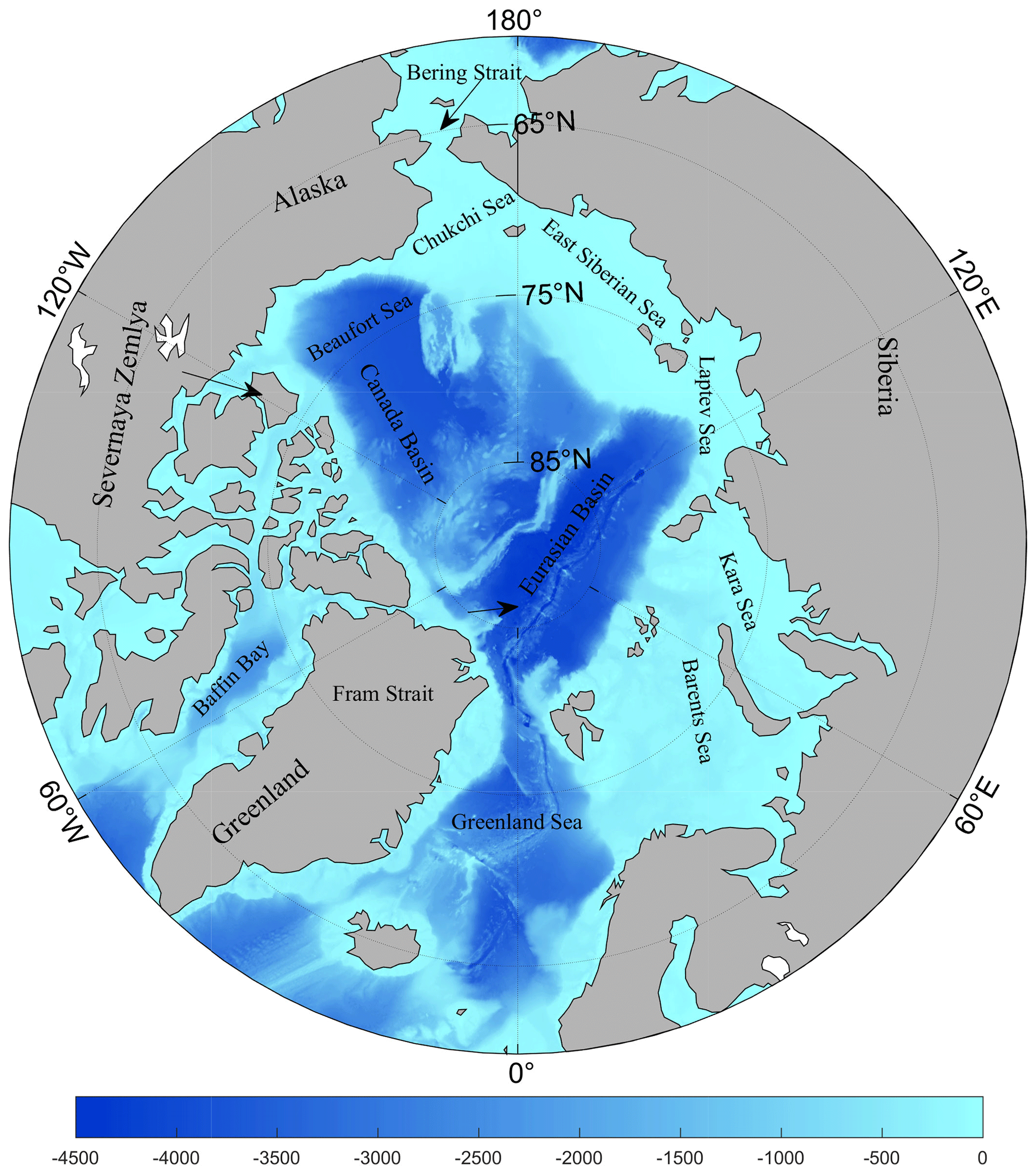
Figure 1Geographic map of the Arctic and its adjacent seas (the shading represent the water depth in meters).
2.1 Data
The sea ice movement data used in this paper are the mean monthly gridded sea ice motion vector products released by the National Snow and Ice Data Center (NSIDC). We chose the Polar Pathfinder Monthly 25 km EASE-Grid Sea Ice Motion Vectors (Version 4) (Tschudi et al., 2019) data because of their homogeneous spatial coverage and long-term availability. These data are obtained by combining the data observed from Advanced Very High Resolution Radiometer, Scanning Multichannel Microwave Radiometer, Special Sensor Microwave/Imager and International Arctic Buoy Program measured data. The time span is from January 1979 to December 2018. The data are projected on an equal-area map with a spatial resolution of 25 km, covering the entire area from 48.4 to 90∘ N.
To understand the relationship between geophysical variables and the variation characteristics of multiscale sea ice movement, 10 m sea level wind field (SLWF), mean sea level pressure (MSLP) and sea surface temperature (SST) data released by the European Centre for Medium-Range Weather Forecasts (ECMWF) are also selected for correlation analysis. The time span of these data is the same as that of the sea ice motion, and the spatial resolution is . Additionally, we also use the sea ice concentration (SIC) data (Cavalieri et al., 1996) released by the NSIDC, and the time span and spatial resolution of these data are the same as those of the sea ice motion data.
2.2 Method
2.2.1 Statistical analysis of sea ice drift patterns
The empirical orthogonal function (EOF) analysis method is a widely used multivariate statistical technique used to investigate spatial patterns of variability and how they change with time (Iida and Saitoh, 2007). In this study, we employed the EOF method to extract the spatial patterns of sea ice drift over 40 winter season datasets from 1979 to 2018. The EOF method yields eigen-patterns of variability and corresponding principal component time series for spatiotemporal data analysis. To facilitate the calculation of the vector dataset, we convert the three-dimensional matrix to a two-dimensional matrix. The three-dimensional matrix was arranged such that the spatial components were in the first two dimensions and the temporal components were in the third dimension. Then, zonal and meridional components of the ice drift motion were arranged underneath each other to form a single matrix, in which rows 1–361 indicate the zonal component and rows 362–722 indicate the meridional component. Finally, we multiplied the result by −1 to obtain the vectors in the correct directions.
2.2.2 Mann–Kendall (MK) nonparametric statistical trend test
In this paper, the monotonic variation trend of the time series of sea ice motion vector data is analyzed by the Mann–Kendall (MK) nonparametric test method. This method does not require data to conform to a normal distribution and is not affected by a small number of outliers and missing values, so it is widely used in the trend analysis of hydrological and ocean data (Vantrepotte and Melin, 2011).
2.2.3 Hilbert–Huang transform (HHT)
The Hilbert–Huang transform (HHT) is a newly developed adaptive time-frequency analysis method with high efficiency (Huang et al., 1998). It can process nonlinear and nonstationary data and is widely used in various geophysical studies (Huang and Wu, 2008). The HHT consists of two parts: empirical mode decomposition (EMD) and Hilbert transform (HT). EMD is a signal decomposition method that decomposes the original time series data into intrinsic mode functions (IMFs) from high-frequency components to low-frequency components. These IMFs must have two characteristics: (1) the number of extremum points is equal to or at most one different from the number of zero crossings, and (2) the average value of the upper envelope formed by the local maximum value and the lower envelope formed by the local minimum value is zero. Only in this way can the calculated IMFs maintain the physical significance of amplitude and frequency modulation.
However, EMD may result in pattern confusion, which is mainly manifested as a single IMF containing signals of different timescales or a signal of similar scales appearing in different IMFs. Such a result allows the decomposed IMF to lose its original physical meaning. To solve this problem, Huang (2004) proposed the ensemble empirical mode decomposition (EEMD) method, which adds white noise with limited amplitude to the original data signal and magnifies the extreme value points of the original signal through noise, largely reducing the uncertainty due to confusion. The EEMD method is used in this paper. The amplitude of the white noise is 0.2 times the maximum amplitude of the original signal, and the ensemble number is set to 600.
To judge whether the IMF is noise information or a result with physical significance, the significance test should be carried out according to the distribution characteristics of the average period and the energy of each IMF (Fig. 2). If the decomposed energy of the IMF is distributed above the confidence level, it is considered to have actual physical significance; otherwise, it is considered to be white noise.
To ensure that an IMF for EEMD includes a useful signal, we test the statistical significance of the IMFs based on the method proposed by Wu and Huang (Huang, 2004).
-
Calculate the energy of the IMFs. The energy of the nth IMF can be written as follows: , where Ck is the nth IMF and K is the number of data points.
-
Ascertain any specific IMF containing little useful information, assume that the energy of that IMF comes solely from noise, and assign it to the 95 % line.
-
Use the energy level of that IMF to rescale the rest of the IMFs.
-
If the energy level of any IMF lies above the theoretical reference white noise line, we can safely assume that this IMF contains statistically significant information. If the rescaled energy level lies below the theoretical white noise, then we can assume that the IMF contains little useful information.
Figure 2a shows the significance testing of the first EOF pattern temporal coefficient series with white noise analysis. As seen from the figure, all IMFs of the decomposition results are located below the 95 % confidence line and therefore are considered as noise information. Obviously, such a test result is unreasonable. Data such as SST data have autocorrelation, a large trend and possibly noise other than Gaussian white noise. Therefore, the white noise test should not be used in the test, and the red noise test should be used instead. The test results of the first EOF pattern temporal coefficient series, which likely contains other types of noise, seem to exaggerate the significance of some IMFs. To eliminate this problem, methods that can test against other types of noise (red noise) should be used (Huang and Shen, 2005). Figure 2b shows the significance testing of the first EOF pattern temporal coefficient series with red noise analysis. All IMFs of the decomposition results are located above the 95 % confidence line.
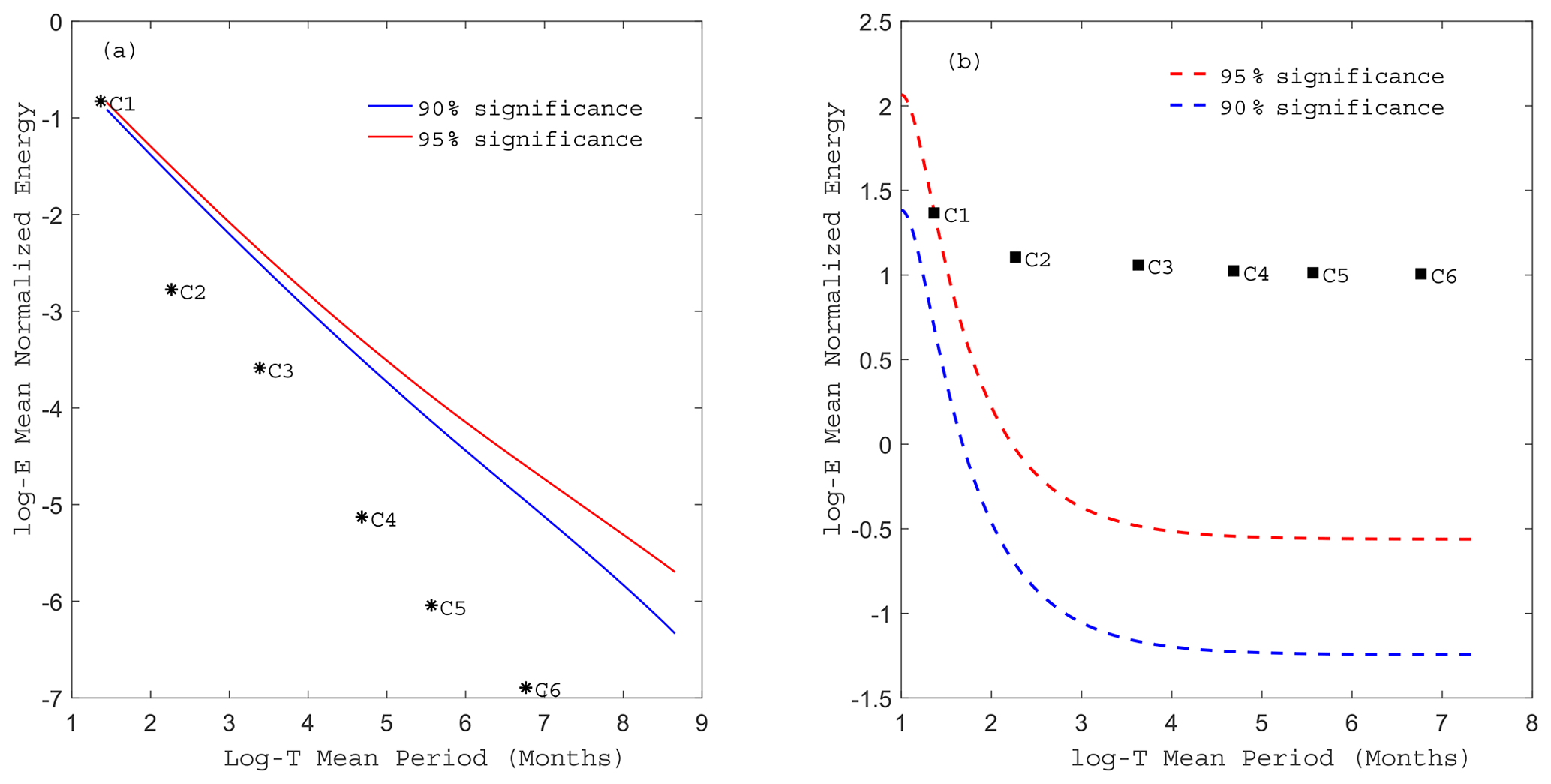
Figure 2Statistical significance test of six IMFs of the first EOF pattern temporal coefficient series with white noise (a) and red noise (b). Each symbol represents the mean normalized energy of an IMF as a function of the mean period of the IMF, ranging from the first IMF to the sixth IMF. The red line represents the 95 % confidence level, and the blue line is the 90 % confidence level.
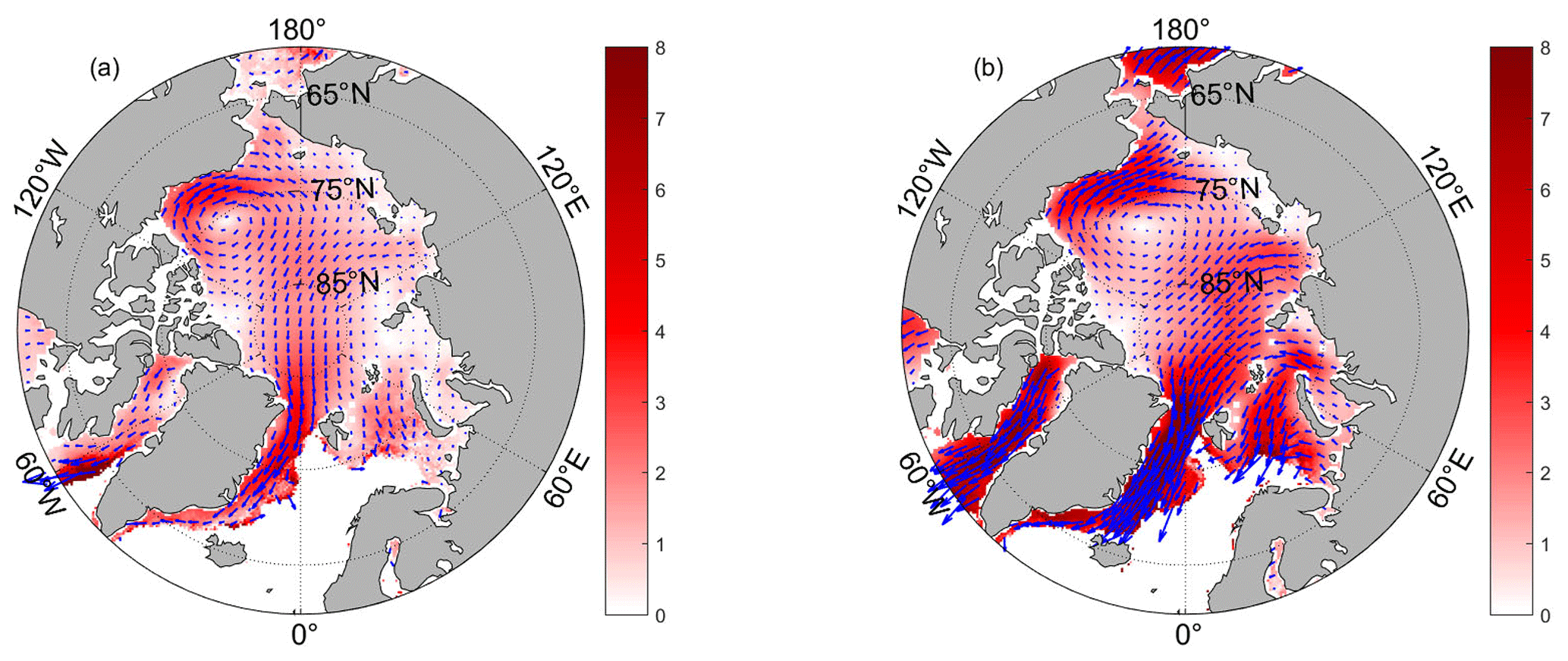
Figure 3Climatological distribution of the sea ice drift speed field in summer (a) and winter (b) from 1979 to 2018 (the different shading represents the velocity, and the arrows represent the direction and magnitude of ice drift).
3.1 Climatological distribution characteristics
Based on the 40-year (1979–2018) monthly mean sea ice motion data, the climatological distributions of the sea ice drift velocity field in summer (May–October) and winter (November–April) are presented. The results show the difference in the magnitude and direction of the sea ice drift between winter and summer. In general, the main pattern of Arctic sea ice drift is anticyclonic motion in the Beaufort Sea, i.e., the BG and TPD, which drives ice from the Laptev Sea across the pole to the Fram Strait. The Arctic sea ice drift in winter (Fig. 3b) and summer (Fig. 3a) have the same dominant circulation patterns, but winter is stronger than summer. The above indicates that even if we use only the winter months dataset, we can describe the large-scale circulation regimes and their variability in Arctic sea ice motion over time very well. In the following analysis, in order to allow the sea ice motion dataset better continuity in spatial and temporal distribution, we found that the data from November to April had a relatively high coverage rate in each month in the whole period from 1979 to 2018.

Figure 4Annual spatial distribution of monotonic variation trends in sea ice motion from 1979 to 2018. (a) The zonal component of drift speed (red shading values indicate enhanced eastward drift, while blue shading values indicate enhanced westward drift, where east is counterclockwise), (b) the meridional component of drift speed (red shading values indicate enhanced northward drift, while blue shading values indicate enhanced southward drift, where north is toward the center of the grid), and (c) total drift velocity (red shading values indicate drift velocity increases, while blue shading values indicate drift velocity decreases). The significance test was carried out by the Mann–Kendall nonparametric test (p<0.05).
3.2 Monotonic trend
To obtain the monotonic trend of sea ice drift motion in the Arctic Ocean, monotonic trend analysis from 1979 to 2018 was carried out at each grid point using the MK nonparametric test method. Figure 4 shows the monotonic variation trend of the sea ice motion (Fig. 4c) and its zonal (Fig. 4a) and meridional (Fig. 4b) components are available for the period from 1979 to 2018. As shown in Fig. 4a, the sea ice drift of the zonal component is a significant feature in the Beaufort Sea, which shows an obvious decreasing trend, with an average annual decrease of more than 6 cm. These trends indicate a strengthening of the anticyclonic sea ice drift pattern in the Beaufort Sea. Similarly, the sea ice drift of the zonal component shows a negative trend in some areas around the Eurasian Basin and through the Fram Strait, with an average annual decline rate of less than 5 cm. These trends indicate enhanced westward drift, which is consistent with the research results of (Van Angelen et al., 2011) that there is a persistent west–east pressure gradient over the Fram Strait, with the associated northerly geostrophic wind over the Greenland Sea (Van Angelen et al., 2011). The rest of the study area shows an increasing trend, and the Laptev Sea, Canadian Basin and Baffin Bay all exhibited an annual increase of approximately 5 cm. For the meridional component of drift speed (Fig. 4b), the positive and negative pattern distributions in the Beaufort Sea area once again reinforce the anticyclonic sea ice drift pattern. The sea ice drift in the Beaufort Strait and Baffin Bay has a strong southward trend, with an average annual change of more than 5 cm. This indicates that the sea ice export from the Canadian Basin and the Arctic to Baffin Bay shows an increasing trend year by year. However, in the Kara Sea and Laptev Sea regions, an enhanced poleward flow is observed, which shows a strengthening trend of TPD from 1978 to 2018.
In general, as seen from Fig. 4c, the total drift velocity of Arctic sea ice shows an increasing trend over the time series, except for a slight weakening trend in some parts of the Bering Strait. Especially in the Beaufort Sea, Kara Sea (KS) and both sides of Greenland (Baffin Bay and the Fram Strait), the sea ice drift rate changes significantly, and it strongly affects the spatial and temporal distribution of sea ice in the Arctic Ocean. Thus, it can be seen that the variation trend of sea ice drift patterns in the Arctic Ocean is not uniform and consistent, and both the BG and TPD drift patterns show high rates of change.
3.3 EOF spatiotemporal characteristic
As mentioned above, the distribution of summer sea ice is vulnerable to the effects of weather, atmospheric moisture, and surface melting, which have a detrimental effect on the data quality and analysis (Sumata et al., 2015). Therefore, this study uses the sea ice drift data in the winter periods of 1979–2018 for EOF analysis to obtain the temporal and spatial patterns of sea ice drift and then conducts multiscale analysis on the temporal variations in the main spatial distribution patterns of sea ice drift.
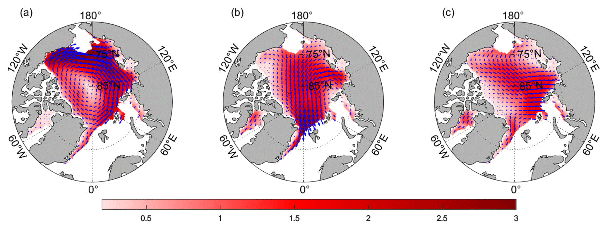
Figure 5The characteristic vectors for the EOF-based first pattern (a), the second pattern (b) and the third pattern (c) of the Arctic sea ice motion in winter from 1979 to 2018.
The spatial distributions of the first three patterns, as shown in Fig. 5, are similar to those of the three significant sea ice drift patterns. The first EOF pattern (Fig. 5a) shows an anticyclonic circulation of sea ice drift around the entire Arctic Ocean. The second EOF pattern (Fig. 5b) is similar to the average sea ice transport patterns and shows the export of sea ice from the BG and TPD to the Fram Strait. The third EOF pattern (Fig. 5c) shows the drift of the sea ice transport system moving ice between the KS and the northern coast of Alaska. However, the first two EOF patterns are the two dominant Arctic circulation patterns of sea ice drift and account for 30.2 % and 19.1 % of the total variance, respectively. The variance contribution of the third pattern is only 11.0 %. This pattern of ice drift is observed by using 3 years (1979–1981) of drifting buoy data, which show a reversed TPD stream over a 30 d period in summer (Serreze et al., 2013).
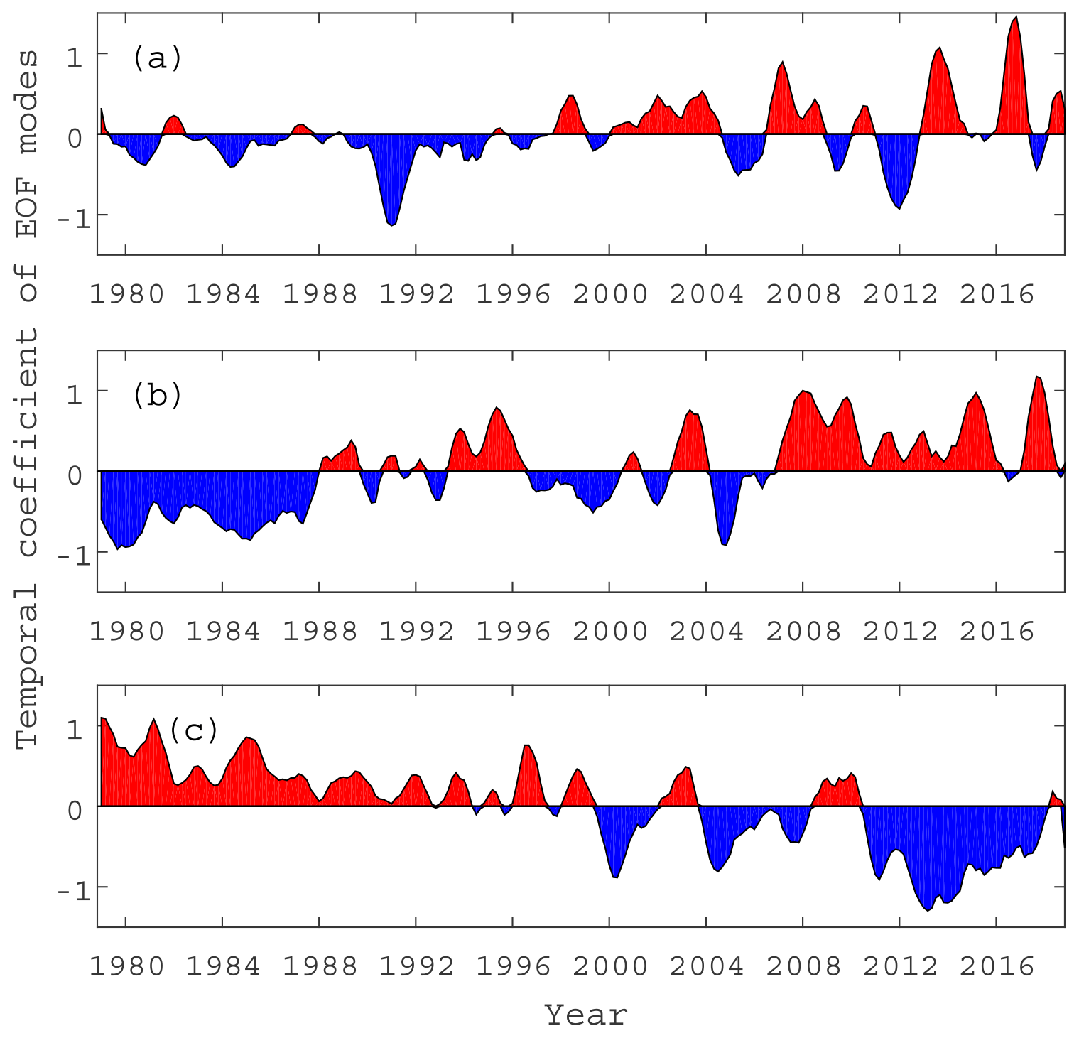
Figure 6The corresponding EOF-based temporal coefficients of the Arctic sea ice motion in winter from 1979 to 2018.
The combination of these data with the temporal coefficients by EOF (Fig. 6) reveals that when the modes are in the positive phase (red series in Fig. 6), the dominant Arctic circulation patterns of sea ice drift exhibit the same pattern as illustrated in Fig. 5. However, when the modes are in the negative phase, the sea ice drifting patterns in these years (blue series in Fig. 6) are the opposite of those in Fig. 5. This pattern of ice drift mainly manifests itself as cyclonic drift with a large-scale counterclockwise ice motion pattern that tends to prevail in summer, and the sea ice export from the Fram Strait is low or even negative. The first pattern of corresponding temporal coefficients (Fig. 6a) shows that before 1997, the drifting pattern of sea ice was mainly cyclonic circulation or weak anticyclonic circulation, while after 1997, the drifting pattern was mainly anticyclonic circulation, which is similar to the current winter drifting pattern. Among them, the anticyclonic sea ice drift circulation appeared the weakest in approximately 1991, while the anticyclone circulation appeared the strongest in approximately 2013 and 2017. We can see from the temporal coefficients of the second EOF pattern (Fig. 6b) that the export of sea ice from the BG and TPD to the Fram Strait shows three main periods in the time series. Before 1988, it was dominated by negative modes; after 2007, it was dominated by positive modes and fluctuated between positive and negative modes over time between 1988 and 2007. The third pattern of temporal coefficients (Fig. 6c) shows an opposite trend from the first EOF pattern. Before 2000, it was basically a positive mode, and then it was mainly a negative mode.
The above analysis of EOF spatial and temporal modes allows us to show the variations in the patterns of Arctic sea ice drift retrieved by applying the EOF analysis for the period from 1979 to 2018. Next, we use multiscale analysis to analyze the variation characteristics of each EOF pattern in more detail.
3.4 Multiscale variation characteristic
3.4.1 Multiscale variation characteristics of each EOF pattern
To analyze the multiscale variation characteristics of each EOF pattern (Fig. 5), we performed EEMD decomposition on the temporal coefficients obtained from EOF analysis (Fig. 7) and obtained the IMF modes and trend components that represent the characteristics of the interannual variations and long-term variation trends of the three main drift patterns of sea ice. Then, we explored the relationship between the sea ice drift pattern and atmospheric and oceanic forcing on different temporal scales. Among them, the first high-frequency mode of all IMFs reflects the situation of seasonal oscillation. Since we use the data of the Arctic winter months (November–April), the time resolution of the analysis of seasonal oscillation is insufficient, so it is not taken into account here. The decomposition results show that except for the first mode of all IMFs, the second mode accounts for the highest variance contribution, followed by the third mode (Table 1). Due to the complexity of the factors (atmospheric and oceanic forcing factors) that relate to Arctic sea ice drift, there are few rigorous quasi-annual cyclic modes of sea ice drift circulation patterns.
Table 1The period and variance contribution rate of each IMF mode
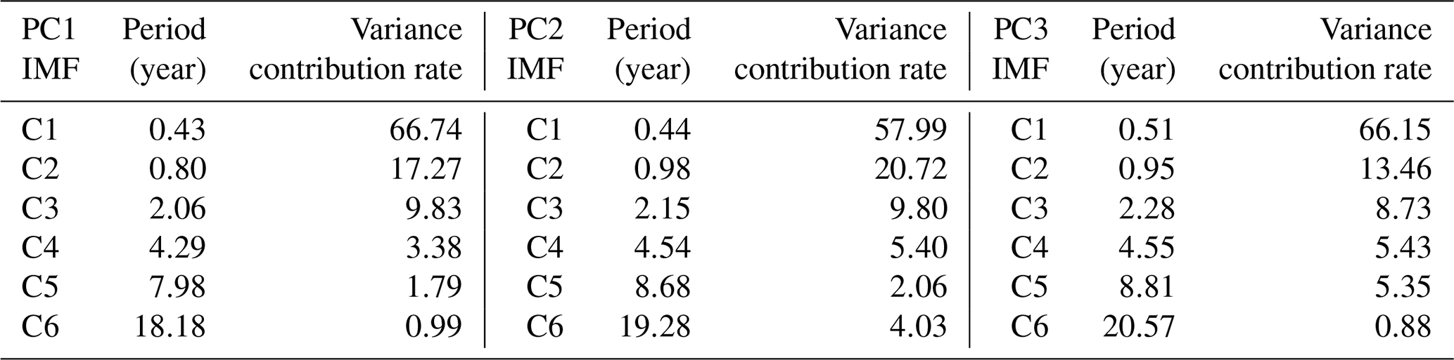
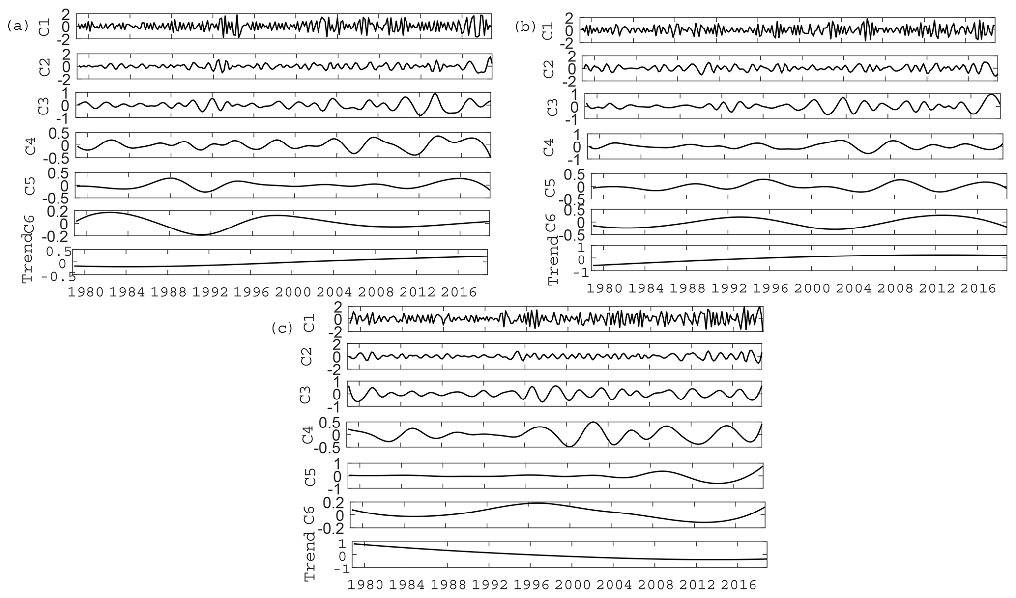
Figure 7The IMF modes and trend components after EEMD of the first EOF temporal coefficient (a), the second EOF temporal coefficient (b) and the third EOF temporal coefficient (c).
Figure 7 shows the IMF modes and trend components of the three main EOF temporal coefficient series for Arctic sea ice drift data after EEMD decomposition. The EOF temporal coefficient series data used in the analysis included data from 240 winter months which were decomposed into six timescales (marked C1–C6 in Fig. 7) and one trend component (marked trend in Fig. 7) by the EEMD method.
For the interannual variation in the Arctic sea ice drift patterns, except for the removal of the first mode, the periods of the other IMF modes from C2 to C5 are approximately 1 year, 2 years, 4 years and 8 years, respectively, and the oscillation of each IMF curve is not stable; some years have large amplitude changes, and some years have no obvious amplitude changes. Moreover, the oscillation frequency of each timescale curve of the first EOF drift pattern is faster than that of the latter two patterns. As seen from the contribution rate of the covariance value, the significance of the high-frequency oscillation (C2–C3) in the first pattern and the second pattern is relatively strong, while that in the third pattern is obviously much weaker. However, the third pattern of medium-frequency oscillation (C4–C5) is more significant (Table 1). Therefore, we cannot simply consider the Arctic sea ice drift as a single pattern. The three patterns extracted by EOF analysis, representing the Arctic main sea ice drift patterns, have different multiscale oscillation characteristics, and the movement of sea ice drift is related to many factors. Moreover, the intensity of each factor is also different, resulting in different amplitudes in each year. For example, it can be seen from Fig. 7a that the first major pattern of sea ice drift showed a greater range of multiyear fluctuations in approximately 1992 than in other years.
For the interdecadal variation, the periods of C6 are approximately 18, 19 and 21 years, which can be used to show interdecadal changes in sea ice drift patterns for each EOF pattern. From the variance contribution rate of each timescale in Table 1, it can be seen that the C6 variance contribution rate of the second EOF temporal coefficient series is 4.03, which is relatively high, while the C6 contribution rate of the first and third EOF temporal coefficient series is relatively low. This indicates that the long period oscillation of the second EOF ice drift circulation pattern is more obvious, while the short period oscillation within 10 years of the other two EOF ice drift circulation patterns is more obvious.
For the trend variation, the residual components of the original EOF temporal series coefficient data after EEMD decomposition are the trend components. The decomposition results show that the first two EOF circulation patterns show an increasing trend variation, while the third circulation pattern decreases year by year (Fig. 7). Together with the monotonic trend analysis in Fig. 4, we can determine that there is an enhanced anticyclonic sea ice drift pattern and a strengthening trend of TPD from 1978 to 2018. That is, the anticyclonic circulation around the Arctic basin and the flow through the North Pole reflect the two main drift patterns of the current Arctic sea ice drift, and the sea ice output through the Fram Strait shows an increasing trend year by year. Other patterns include the third EOF pattern of sea ice drift, which reflects the occasional occurrence of sea ice drift in individual years or summer showing a downward trend.
Through the above analysis of the multiple timescales of the major sea ice drift patterns, we understand the characteristics of the multiple-year timescale, including more than 10 years (interdecadal), of the sea ice drift patterns in the Arctic and the trend in the whole time series. In the following section, we discuss in detail the atmospheric or oceanic forcing factors which are the main factors relating to the Arctic sea ice drift circulation patterns.
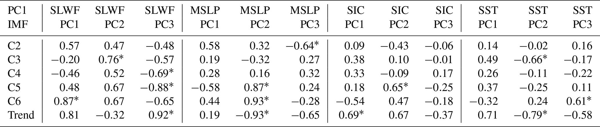
Table 2The correlations between the first EOF sea ice drift pattern on various timescales and environmental factors (the PCs with the highest correlation values greater than 0.6 are marked with an asterisk).
Based on the above analysis of our long time series data on Arctic sea ice drift, we know that the Arctic sea ice drift has significant spatial and temporal differences. Moreover, the three EOF sea ice drift patterns have different multiscale variation characteristics, and all of them have strong interannual variation characteristics. Among them, the second pattern has significant interdecadal change characteristics, while the other two patterns have no obvious interdecadal change characteristics.
However, what factors cause Arctic sea ice drift to have some of the above variation characteristics? Previous studies (Wang and Zhao, 2012) have shown that the variation in the Arctic atmospheric environment is the main factor affecting the variation in sea ice drift, and the wind field or atmospheric pressure field (Lindsay et al., 2009) affects the transport of Arctic sea ice. According to the dynamic equation of sea ice drift (Leppäranta, 2011), sea surface conditions also have an important influence on the speed of sea ice drift. Studies have shown that sea ice density is an important parameter of sea surface roughness in the Arctic Ocean (Yu et al., 2020), and it has an important influence on the speed of sea ice drift, especially in the marginal sea area of the Arctic Ocean.
To discuss the correlation between various timescales of Arctic sea ice drift pattern change from 1979 to 2018 and the atmospheric or oceanic force factors, the data of the 10 m SLWF, MSLP, SIC and SST are processed in the same way as the sea ice motion data for correlation analysis. First, the EOF analysis method was used to extract the temporal coefficient series of the first three principal components (PCs), and then EEMD was performed to obtain information of each timescale of the original sequence. Finally, the relationship between the Arctic sea ice drift patterns and these geophysical variables was obtained.
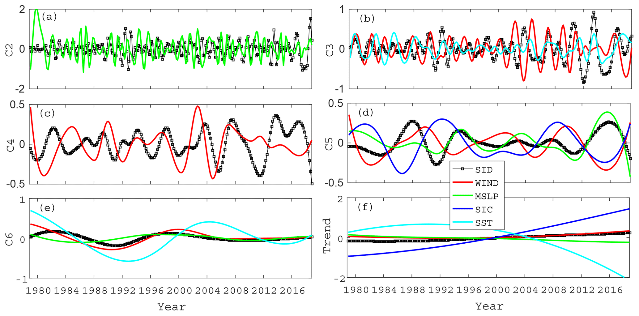
Figure 8The IMF modes (a–e) and trend components (f) after EEMD of the first sea ice EOF temporal coefficient and each environmental parameter. (For each environmental parameter, only the EOF component marked with an asterisk is drawn.)
The first EOF pattern, which represents anticyclonic circulation of the sea ice drift around the entire Arctic Ocean (Fig. 5a), is one of the main patterns of Arctic winter sea ice drift. The drift pattern is a large-scale anticyclonic circulation across the entire Arctic Ocean. The main environmental factors that correlate with its development are the large-scale atmospheric circulation of the Arctic, so the SLWF and MSLP have a large influence on this ocean-scale circulation, while the ocean environmental factors mainly correlate with the regional oceans and have a weak correlation with this sea ice drift pattern.
The direct correlation between the first Arctic sea ice drift pattern on various timescales and environmental factors are shown in Table 2. It can be clearly seen that the correlation coefficient of atmospheric parameters is basically greater than that of oceanic parameters. We chose a principal component of these four geophysical variables marked with stars, which have the greatest correlation with sea ice movement, and the correlation value is greater than 0.6 (when the coefficient is greater than 0.6, the two parameters have a strong correlation). It can be seen more clearly that the atmospheric environment plays a leading role in sea ice drift, especially for the long period oscillations of 8 (C5) and 18 (C6) years, and their correlation coefficients are all greater than 0.8. Combined with Fig. 8, we can see that atmospheric forcing has a dominant effect on sea ice drift in the whole time period, while oceanic forcing only plays a limited role in a few periods. For example, it can be seen from Fig. 8b that only from 2012 to 2016 did the sea ice drift movement fluctuate greatly, during which SST played a leading role in its change, while the wind field played a leading role in other periods. Moreover, sea ice drift has a hysteresis effect on the corresponding forcing factors. The oscillation delay effect is more obvious with lower frequency, and the delay time even reaches half a period in some time periods (Fig. 8b from 2002 to 2006).
As shown in the previous results, the anticyclone circulation appeared to be the strongest in around 2013 and 2017. As shown in Fig. 8b, this phenomenon is quite significant, and the oscillation is more pronounced in the timescale series with a period of 2 years (C3). Moreover, the dominant forcing factor is ocean conditions, not atmospheric factors.

Figure 9The IMF modes (a–e) and trend components (f) after EEMD of the second sea ice EOF temporal coefficient and each environmental parameter. (For each environmental parameter, only the EOF component marked with an asterisk is drawn.)
Table 3The correlations between the second EOF sea ice drift pattern on various timescales and environmental factors (the PCs with the highest correlation values greater than 0.6 are marked with an asterisk).
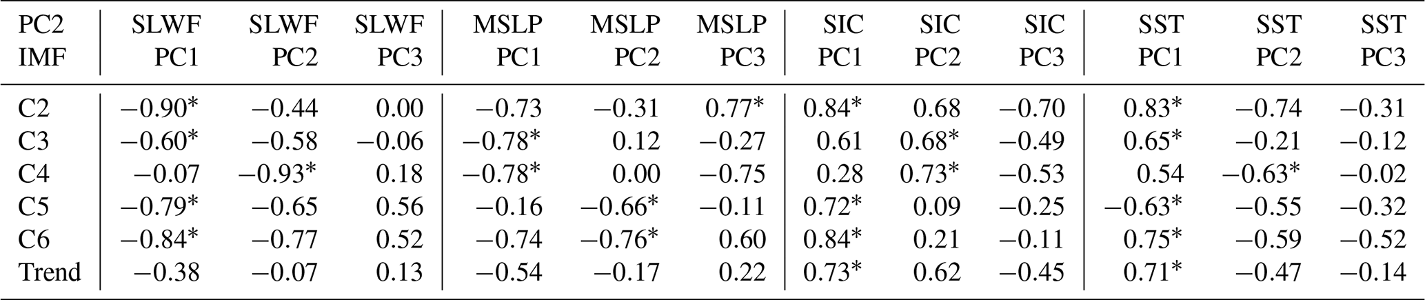
The second EOF pattern, which represents the export of sea ice from the BG and TPD to the Fram Strait (Fig. 5b), is one of the main patterns of Arctic sea ice drift. As seen from Table 3, it is affected by both atmospheric and ocean conditions and is basically affected by the first two PCs of environmental factors. Modeling results show that the wind stress transfer to the ice-covered ocean is maximized at approximately 80 % ice concentration (Martin et al., 2014). Wind stress transfer increases as SIC decreases from 100 % to the threshold concentration because sea ice becomes more mobile while still retaining a high surface roughness. Thus, the decrease in ice concentration during the early summer might also enhance ocean currents and consequentially strengthen the oceanic drag force on the ice, which in turn increases the ice speed.
It is precisely because this pattern of sea ice transport is affected by the joint action of atmospheric and ocean environmental factors that the dominant factors of sea ice movement at different timescales are different in different years. It can be clearly seen from Fig. 9d that in the period from 1988 to 1996 (the period of C5 is 8 years), the sea ice movement is mainly correlated with atmospheric forcing. The temporal curve of sea ice movement is close to the change curve of atmospheric forcing, and the change in sea ice movement is followed by atmospheric forcing. In the subsequent period, the correlation of ocean forcing on sea ice movement gradually strengthened. In the whole time series, the atmosphere and ocean alternately play a dominant role in the movement of sea ice. However, for C6 with significant interdecadal changes, it can be seen from Fig. 9e that, due to the delayed effect of oceanic and atmospheric environmental factors on sea ice movement, the superposition effect of ocean and atmosphere allows for a significant sea ice motion during that period. In the time series, the ocean and atmosphere have roughly equal effects.
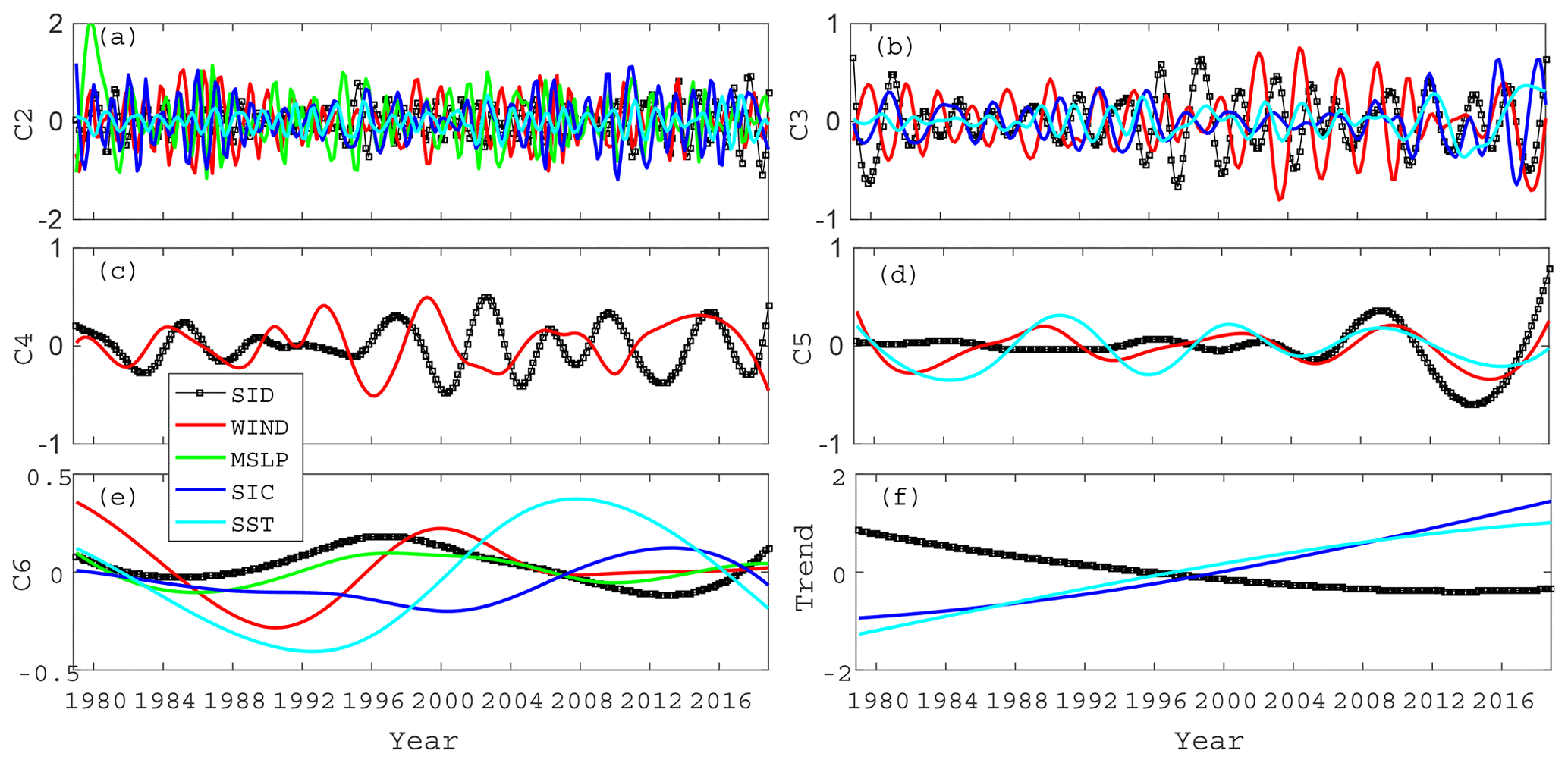
Figure 10The IMF modes (a–e) and trend components (f) after EEMD of the third sea ice EOF temporal coefficient and each environmental parameter. (For each environmental parameter, only the EOF component marked with an asterisk is drawn.)
Table 4The correlations between the third EOF sea ice drift pattern on various timescales and environmental factors (the PCs with the highest correlation values greater than 0.6 are marked with an asterisk).
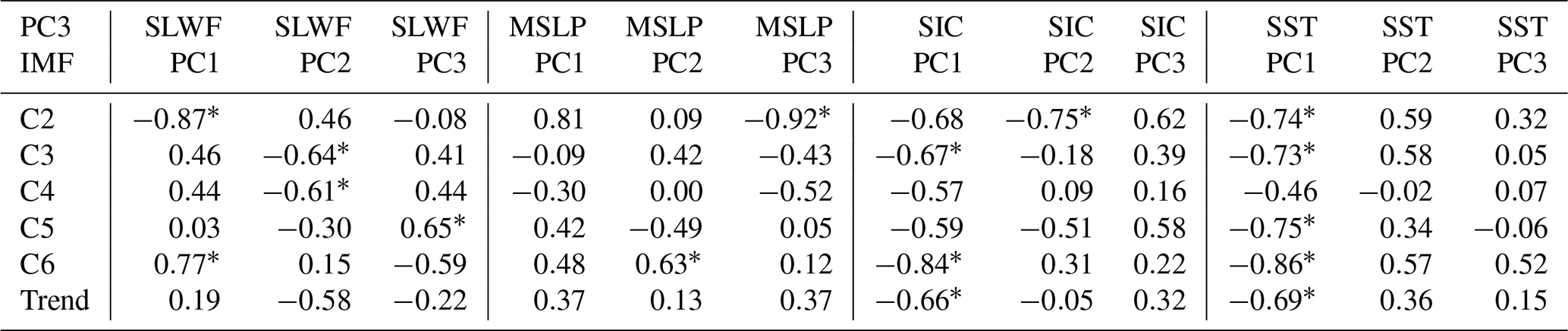
For the third EOF pattern, which represents the sea ice transport system moving ice between the KS and the northern coast of Alaska. The correlation analysis in Table 4 shows that sea ice transport between the KS and the northern coast of Alaska is mainly correlated with the ocean environment. Only the high-frequency oscillation C2 is more correlated with the atmosphere than the ocean environment, but the ocean forcing effect is still relatively large and cannot be ignored. In addition, the correlation of C4 is not high, with the highest correlation being the wind field and the correlation coefficient only being −0.61. Combined with Fig. 10c, it can be seen that before 1990, the sea ice drift movement was basically dominated by the wind field, while later, the forcing effect of the wind field on the sea ice drift was not obvious, and the correlation was low. Especially after 2004, the variation in the sea ice drift curve has little correlation with the wind field curve. From the previous analysis results, we know that after 2000, the third EOF pattern of sea ice drift is mainly a negative mode, that is, sea ice migration from the northern coast of Alaska to the KS. This indicates that the migration pattern of sea ice can reverse due to changes in forcing factors. For other timescales (C3, C5 and C6), the effect of ocean forcing on sea ice movement is greater than that of the atmosphere, especially SST.
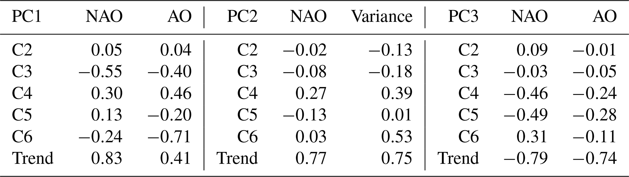
Table 5The correlations between the first three EOF sea ice drift patterns on various timescales and a variety of large-scale atmospheric index.
The trend changes in the second and the third main patterns of Arctic sea ice drift retrieved by applying the EOF analysis are mainly correlated with ocean environmental factors. However, the first main pattern showed a more significant correlation with atmospheric environmental factors. What more, the second EOF pattern representing sea ice output from Fram Strait shows an increasing trend, while the third EOF pattern shows a decreasing trend. This indicates that the export of Arctic sea ice from Fram Strait increases, while that from Bering Strait decreases. However, the export of Arctic sea ice is mainly through Fram Strait, so in general, the export of Arctic sea ice shows an increasing trend in the last decades. With the variation trend of sea ice movement, the Arctic sea ice concentration indicates a decreasing trend in the future, especially from the Eurasian Basin to the Fram Strait. Furthermore, the extent to which sea ice export through Fram Strait controls ice conditions (thickness and motion) upstream of the transpolar drift system and the export influence a large area upstream in the transpolar drift stream, and high volume export events lead to a thinner thickness (Zamani et al., 2019).
Finally, we have added a discussion about the relationship between Arctic sea ice drift and large-scale atmosphere circulation, such as Arctic Oscillation (AO) and North Atlantic Oscillation (NAO). As can be seen from Table 5, the correlation between the three sea ice drift patterns on most of the scale and atmospheric index is low. Among them, the decadal variation (C6) of the first pattern has a high negative correlation with the AO index (correlation coefficient is −0.71), which indicates that an anticyclonic circulation of the sea ice drift around the entire Arctic Ocean has a high correlation with the large-scale Arctic circulation. In addition, the trend changes in the three sea ice movement patterns are highly correlated with the large-scale atmospheric indices, which indicates that the large-scale atmospheric changes have a strong correlation with the changes in sea ice movement patterns, while some high-frequency changes in sea ice movement (interannual and multiyear changes) are not highly correlated with the large-scale atmospheric circulation.
In previous studies on the movement of Arctic sea ice, most believed that the movement of sea ice was mainly forced by the atmospheric environment and highly correlated with the wind field. However, our results suggest that the ocean environment also has a significant relationship with sea ice movement. As the atmospheric environment factor itself changes more frequently than the ocean environment factor, the influence scale is large, the range is wide, and the correlate with the sea ice movement is more intense, which allows the response of the sea ice movement to the atmospheric environment factor to be more obvious and the lag time shorter than the response to the ocean factor. Therefore, the correlation of ocean environmental factors with sea ice movement is masked by the correlation of the atmospheric environment. By analyzing the time series data of sea ice movement on various timescales after decomposition, it is found that the driving effect of ocean environmental factors on sea ice movement is also very important. The correlation of the ocean environment with sea ice movement is not only in the marginal sea area but also in the central sea area of the Arctic Ocean. In some years, its correlation even exceeds the atmospheric environmental forcing, which plays a leading role in sea ice movement.
As discussed above, the analysis of the spatiotemporal patterns of Arctic sea ice circulation is of intrinsic value in identifying and understanding general patterns in the behavior of the atmosphere–ice–ocean system. We know that the atmospheric and ocean environmental factors we use for analysis are relatively easy to obtain compared to sea ice condition parameters and that some large-scale climate signals of the atmosphere or ocean are predictable. The occurrence of signals like El Niño–Southern Oscillation (ENSO) can be predicted 6–12 months in advance. However, large-scale climate fluctuations such as ENSO will affect the atmosphere and ocean environment, thus affecting sea ice conditions. Therefore, our study establishes the relationship between sea ice movement and atmospheric and oceanic factors on different timescales, making it easier to predict future sea ice conditions.
In this study, the climate distribution characteristics of the Arctic sea ice drift is briefly analyzed, and it is revealed that the Arctic sea ice drift motion has significant spatial and temporal variation characteristics. As a follow-up study, the multiscale change characteristics of sea ice and the relationship between the geophysical variables were established. Then, the MK nonparametric test was used to determine the spatial distribution of the monotonically changing trend of Arctic sea ice drift. Based on the above analysis of the basic state of Arctic sea ice drift, we performed a detailed analysis of the multiscale characteristics of Arctic sea ice drift and its influencing mechanism. Accordingly, we draw the following conclusions:
-
Generally, the drift velocity in winter is greater than that in summer. The variation trend of sea ice drift in the Arctic Ocean is not uniform and consistent. The sea ice export from the Canadian Basin to Baffin Bay shows an increasing trend year by year. In the Kara Sea and Laptev Sea regions, an enhanced poleward flow is observed, which shows a strengthening trend of TPD from 1978 to 2018. Moreover, the total drift velocity of Arctic sea ice shows an increasing trend over the time series, except for a slight weakening trend in some parts of the Bering Strait.
-
The spatial and temporal distribution of winter Arctic sea ice drift was obtained by EOF analysis. EOF analysis results show that Arctic sea ice has three main spatial patterns. The first EOF pattern shows an anticyclonic circulation of the sea ice drift around the entire Arctic Ocean. The second EOF pattern is similar to the average sea ice transport pattern, which involves the export of sea ice from the BG and TPD to the Fram Strait. The third EOF pattern shows the drift of the sea ice transport system moving ice between the KS and the northern coast of Alaska.
-
The time coefficients obtained from EOF analysis were decomposed into six timescale series and one trend component by the EEMD decomposition method. The three major patterns have significant interannual-scale variation characteristics of approximately 1, 2, 4 and 8 years. Among them, the second pattern also has a significant interdecadal change characteristic with a period of approximately 19 years, while the other two patterns have no significant interdecadal change characteristics.
-
Finally, through the correlation analysis between the three main EOF patterns of Arctic sea ice drift and geophysical variables, we found that the first pattern is mainly affected by atmospheric environment factors, the second pattern is affected by the joint action of atmospheric and ocean environment factors, and the third pattern is mainly affected by ocean environment factors. This is due to the different regulatory effects of the atmosphere and ocean environment on the movement of the three sea ice drift patterns on various timescales. As a result, the three sea ice drift patterns have different multiscale variation characteristics. The stronger the modulation effect of the atmosphere on the sea ice drift pattern, the more significant the high-frequency oscillation of sea ice drift is and the shorter the oscillation period is. Indeed, our calculations show that the oscillation frequency of the first EOF sea ice drift pattern is higher than that of the third drift pattern.
Our study suggests that the ocean environment also has significant correlations with sea ice movement. Especially for some sea ice transport patterns, the correlation even exceeds atmospheric forcing. Similar to the sensitivity experiment in the numerical model, we can obtain relatively simple signals by decomposing complex time series signals of sea ice movement data, which is more conducive to the correlation analysis of its impact factors, in order to understand the internal mechanism of the correlation of environmental factors (such as atmospheric or oceanic factors) on it. In the original data sequence, the correlation of various environmental factors is often superimposed, and some of the correlate signals are masked, which makes it impossible to conduct effective mechanism analysis.
The sea ice movement data and sea ice concentration data were obtained from the National Snow and Sea Ice Data Center (NSIDC; https://nsidc.org/data/NSIDC-0116, Tschudi et al., 2020; https://nsidc.org/data/NSIDC-0051/, Cavalieri et al., 1996). The ERA-Interim data were obtained from the European Centre for Medium-Range Weather Forecasts (ECMWF; https://apps.ecmwf.int/datasets/data/era40-moda/levtype=sfc/, Kållberg et al., 2004).
DF contributed to the conception of the study. HH and LQ assisted with satellite data collection and processing. BL contributed significantly to the analysis and manuscript preparation, performed the data analyses, and wrote the manuscript. GY and YQ helped perform the analysis with constructive discussions.
The authors declare that they have no conflict of interest.
Publisher’s note: Copernicus Publications remains neutral with regard to jurisdictional claims in published maps and institutional affiliations.
This work was supported by Key projects of the Guangdong Education Department under grant 2019KZDXM019, by the fund of the Southern Marine Science and Engineering Guangdong Laboratory (Zhanjiang) under grant ZJW-2019-08, by the high-level marine discipline team project of Guangdong Ocean University under grant 002026002009, by Guangdong graduate academic forum project under grant 230420003, and by the “first class” discipline construction platform project in 2019 of Guangdong Ocean University under grant 231419026.
This research has been supported by the Science and Technology Planning Project of Guangdong Province of China (grant no. 2016A020222016), the Guangdong Education Department (grant no. 2019KZDXM019), the Southern Marine Science and Engineering Guangdong Laboratory (Zhanjiang) (grant no. ZJW-2019-08), the high-level marine discipline team project of Guangdong Ocean University (grant no. 002026002009), by Guangdong graduate academic forum project (grant no. 230420003), and the “first class” discipline construction platform project in 2019 of Guangdong Ocean University (grant no. 231419026).
This paper was edited by Daniel Feltham and reviewed by two anonymous referees.
Bader, J., Mesquita, M. D. S., Hodges, K. I., Keenlyside, N., Østerhus, S., and Miles, M.: A review on Northern Hemisphere sea-ice, storminess and the North Atlantic Oscillation: Observations and projected changes, Atmos. Res., 101, 809–834, 2011. a
Bi, H., Sun, K., Zhou, X., Huang, H., and Xu, X.: Arctic Sea Ice Area Export Through the Fram Strait Estimated From Satellite-Based Data: 1988–2012, IEEE J. Sel. Top. Appl., 9, 1–14, https://doi.org/10.1109/JSTARS.2016.2584539, 2016. a
Bi, H., Wang, Y., Xu, X., Liang, Y., Huang, J., Liu, Y., Fu, M., and Huang, H.: Satellite-observed sea ice area flux through Baffin Bay: 1988–2015, The Cryosphere Discuss., 1–28, https://doi.org/10.5194/tc-2018-136, 2018. a
Boutin, G., Lique, C., Ardhuin, F., Rousset, C., Talandier, C., Accensi, M., and Girard, F.: Towards a coupled model to investigate wave-sea ice interactions in the Arctic marginal ice zone, The Cryosphere, 14, 709–735, https://doi.org/10.5194/tc-14-709-2020, 2020. a
Cavalieri, D. J., Parkinson, C., Gloersen, P., and Zwally, H.: Sea ice concentrations from Nimbus-7 SMMR and DMSP SSM/I-SSMIS passive microwave data,Version 1, Boulder, Colorado USA, NASA DAAC at the National Snow and Ice Data Center [data set], 25, 1091, https://doi.org/10.5067/8GQ8LZQVL0VL, 1996. a
Cheng, X. and Xu, G.: The integration of JERS-1 and ERS SAR in differential interferometry for measurement of complex glacier motion, J. Glaciol., 52, 80–88, https://doi.org/10.3189/172756506781828881, 2006. a
Deser, C. and Teng, H.: Evolution of Arctic sea ice concentration trends and the role of atmospheric circulation forcing, 1979–2007, Geophys. Res. Lett., 35, L02504, https://doi.org/10.1029/2007GL032023, 2008. a
Guarino, M. V., Sime, L., Schreder, D., Malmierca-Vallet, I., Rosenblum, E., Ringer, M., Ridley, J., Feltham, D., Bitz, C., Steig, E., Wolff, E., Stroeve, J., and Sellar, A.: Sea-ice-free Arctic during the Last Interglacial supports fast future loss, Nat. Clim. Change, 10, 1–5, https://doi.org/10.1038/s41558-020-0865-2, 2020. a
Hakkinen, S., Proshutinsky, A., and Ashik, I.: Sea ice drift in the Arctic since the 1950s, Geophys. Res. Lett., 35, 116–122, 2008. a
Howell, S. E. L., Komarov, A. S., Dabboor, M., Montpetit, B., Brady, M., Scharien, R. K., Mahmud, M. S., Nandan, V., Geldsetzer, T., and Yackel, J. J.: Comparing L-and C-band synthetic aperture radar estimates of sea ice motion over different ice regimes, Remote Sens. Environ., 204, 380–391, 2018. a, b
Huang, N. and Shen, S.: Hilbert-Huang Transform and Its Applications [M], Interdiscip. Math. Sci., 5, 107–127, https://doi.org/10.1142/5862, 2005. a
Huang, N., Shen, Z., Long, S., Wu, M., Shih, H., Zheng, Q., Yen, N., Tung, C.-C., and Liu, H.: The empirical mode decomposition and the Hilbert spectrum for nonlinear and non-stationary time series analysis, Proc. Roy. Soc. Lond. Ser. A, 454, 903–995, https://doi.org/10.1098/rspa.1998.0193, 1998. a
Huang, N. E. and Wu, Z.: A review on Hilbert-Huang transform: Method and its applications to geophysical studies, Rev. Geophys., 46, RG2006, https://doi.org/10.1029/2007RG000228, 2008. a
Huang, W. N. E.: A Study of the Characteristics of White Noise Using the Empirical Mode Decomposition Method, Proceedings Mathematical Physical and Engineering Sciences, 460, 1597–1611, 2004. a, b
Iida, T. and Saitoh, S. I.: Temporal and spatial variability of chlorophyll concentrations in the Bering Sea using empirical orthogonal function (EOF) analysis of remote sensing data, Deep-Sea Res. Pt. II, 54, 2657–2671, 2007. a
Kållberg, P., Simmons, A., Uppala, S., and Fuentes, M.: The ERA-40 archive [data set], p. 31, available at: https://www.ecmwf.int/node/10595 (last access: 29 April 2020), 2004.
Kaur, S., Ehn, J. K., and Barber, D. G.: Pan-arctic winter drift speeds and changing patterns of sea ice motion: 1979–2015, Polar Record, 54, 1–9, 2019. a
Kawaguchi, Y., Hutchings, J. K., Kikuchi, T., Morison, J. H., and Krishfield, R. A.: Anomalous sea-ice reduction in the Eurasian Basin of the Arctic Ocean during summer 2010, Polar Ence, 6, 39–53, 2012. a
Kwok, R.: Outflow of Arctic Ocean Sea Ice into the Greenland and Barents Seas: 1979–2007, J. Clim., 22, 2438–2457, https://doi.org/10.1175/2008JCLI2819.1, 2009. a
Kwok, R. and Cunningham, G.: Deformation of the Arctic Ocean ice cover after the 2007 record minimum in summer ice extent, Cold Reg. Sci. Technol., 76, 17–23, https://doi.org/10.1016/j.coldregions.2011.04.003, 2012. a
Kwok, R., Spreen, G., and Pang, S.: Arctic sea ice circulation and drift speed: Decadal trends and ocean currents, J. Geophys. Res.-Atmos., 118, 2408–2425, 2013. a
Lannuzel, D., Moreau, S., Meiners, K., Fripiat, F., Wongpan, P., Vancoppenolle, M., Miller, L., Stefels, J., van Leeuwe, M., Flores, H., and Tedesco, L.: The future of Arctic sea-ice biogeochemistry and ice-associated ecosystems, Natu. Clim. Change, 10, 983–992, 2020. a
Leppäranta, M.: The drift of sea ice, Springer Science & Business Media, Springer, Berlin, Heidelberg, https://doi.org/10.1007/978-3-642-04683-4, 2011. a
Lindsay, R. W., Zhang, J., Schweiger, A., Steele, M., and Stern, H.: Arctic Sea Ice Retreat in 2007 Follows Thinning Trend, J. Clim., 22, 165–176, 2009. a
Martin, T., Steele, M., and Zhang, J.: Seasonality and long-term trend of Arctic Ocean surface stress in a model, J. Geophys. Res.-Ocean., 119, 1723–1738, 2014. a
Nghiem, S., Rigor, I., Perovich, D., Clemente-Colón, P., Weatherly, J., and Neumann, G.: Rapid reduction of Arctic perennial sea ice, Geophys. Res. Lett., 34, L19504, https://doi.org/10.1029/2007GL031138, 2007. a
Olason, E. and Notz, D.: Drivers of variability in Arctic sea-ice drift speed, J. Geophys. Res.-Ocean., 119, 5755–5775, https://doi.org/10.1002/2014JC009897, 2014. a
Olonscheck, D., Mauritsen, T., and Notz, D.: Arctic sea-ice variability is primarily driven by atmospheric temperature fluctuations, Nat. Geosci., 12, 430–434, https://doi.org/10.1038/s41561-019-0363-1, 2019. a
Rabe, B., Karcher, M., Kauker, F., Schauer, U., Toole, J. M., Krishfield, R. A., Pisarev, S., Kikuchi, T., and Su, J.: Arctic Ocean basin liquid freshwater storage trend 1992–2012, Geophys. Res. Lett., 41, 8213, https://doi.org/10.1002/2013GL058121, 2014. a
Screen, J., Simmonds, I., and Keay, K.: Dramatic interannual changes of perennial Arctic sea ice linked to abnormal summer storm activity, J. Geophys. Res., 116, D15105, https://doi.org/10.1029/2011JD015847, 2011. a, b
Serreze, M. C., Mclaren, A. S., and Barry, R. G.: Seasonal variations of sea ice motion in the transpolar drift stream, Geophys. Res. Lett., 16, 811–814, 2013. a
Smedsrud, L. H., Sirevaag, A., Kloster, K., Sorteberg, A., and Sandven, S.: Recent wind driven high sea ice area export in the Fram Strait contributes to Arctic sea ice decline, The Cryosphere, 5, 821–829, https://doi.org/10.5194/tc-5-821-2011, 2011. a
Sumata, H., Kwok, R., Gerdes, R., Kauker, F., and Karcher, M.: Uncertainty assessment of Arctic summer ice drift for data assimilation, in: REKLIM workshop, 2015. a
Thomas, D. N.: Sea ice thickness distribution, chap. 2, John Wiley and Sons, Ltd, 42–64, https://doi.org/10.1002/9781118778371.ch2, 2016. a
Thorndike, A. S. and Colony, R.: Sea ice motion in response to geostrophic winds, J. Geophys. Res.-Ocean., 87, 5845–5852, 1982. a
Tschudi, M., Meier, W., Stewart, J., Fowler, C., and Maslanik, J.: Polar Pathfinder daily 25 km EASE-Grid sea ice motion vectors, version 4, dataset 0116, NASA NationalSnow and Ice Data Center Distributed Active Archive Center, Boulder, CO, USA, https://doi.org/10.5067/INAWUWO7QH7B, 2019. a
Tschudi, M. A., Meier, W. N., and Stewart, J. S.: An enhancement to sea ice motion and age products at the National Snow and Ice Data Center (NSIDC), The Cryosphere [data set], 14, 1519–1536, https://doi.org/10.5194/tc-14-1519-2020, 2020. a
Van Angelen, J., Van den Broeke, M., and Kwok, R.: The Greenland Sea Jet: A mechanism for wind-driven sea ice export through Fram Strait, Geophys. Res. Lett., 38, L12805, https://doi.org/10.1029/2011GL047837, 2011. a, b
Vantrepotte, V. and Melin, F.: Inter-annual variations in the SeaWiFS global chlorophyll a concentration (1997–2007), Deep-Sea Res. Pt. I, 58, 429–441, 2011. a
Wang, X. and Zhao, J.: Seasonal and inter-annual variations of the primary types of the Arctic sea-ice drifting patterns, Adv. Polar Sci., 23, 72–81, 2012. a, b
Wu, Z. and Huang, N. E.: A Study of the Characteristics of White Noise Using the Empirical Mode Decomposition Method, Proc. Math. Phys. Eng. Sci., 460, 1597–1611, 2004.
Yu, X., Rinke, A., Dorn, W., Spreen, G., Lüpkes, C., Sumata, H., and Gryanik, V. M.: Evaluation of Arctic sea ice drift and its dependency on near-surface wind and sea ice conditions in the coupled regional climate model HIRHAM–NAOSIM, The Cryosphere, 14, 1727–1746, https://doi.org/10.5194/tc-14-1727-2020, 2020. a, b
Zamani, B., Krumpen, T., Smedsrud, L. H., and Gerdes, R.: Fram Strait sea ice export affected by thinning: comparing high-resolution simulations and observations, Clim. Dynam., 53, 3257–3270, https://doi.org/10.1007/s00382-019-04699-z, 2019. a
Zhang, J., Rothrock, D., and Steele, M.: Recent Changes in Arctic Sea Ice: The Interplay between Ice Dynamics and Thermodynamics, J. Clim., 13, 3099–3114, https://doi.org/10.1175/1520-0442(2000)013<3099:RCIASI>2.0.CO;2, 2000. a