the Creative Commons Attribution 4.0 License.
the Creative Commons Attribution 4.0 License.
 | 12 Aug 2021
Development of a subglacial lake monitored with radio-echo sounding: case study from the eastern Skaftá cauldron in the Vatnajökull ice cap, Iceland
Finnur Pálsson
Magnús T. Gudmundsson
Thórdís Högnadóttir
Cristian Rossi
Thorsteinn Thorsteinsson
Benedikt G. Ófeigsson
Erik Sturkell
Tómas Jóhannesson
We present repeated radio-echo sounding (RES, 5 MHz) on a profile grid over the eastern Skaftá cauldron (ESC) in Vatnajökull ice cap, Iceland. The ESC is a ∼ 3 km wide and 50–150 m deep ice cauldron created and maintained by subglacial geothermal activity of ∼ 1 GW. Beneath the cauldron and 200–400 m thick ice, water accumulates in a subglacial lake and is released semi-regularly in jökulhlaups. The RES record consists of annual surveys conducted at the beginning of every summer during the period 2014–2020. Comparison of the RES surveys reveals variable lake area (0.5–4.1 km2) and enables traced reflections from the lake roof to be distinguished from bedrock reflections. This allows construction of a digital elevation model (DEM) of the bedrock in the area, further constrained by two borehole measurements at the cauldron centre. It also allows creation of lake thickness maps and an estimate of lake volume at the time of each survey, which we compare with lowering patterns and released water volumes obtained from pre- and post-jökulhlaup surface DEMs. The estimated lake volume was 250 GL (gigalitres = 106 m3) in June 2015, but 320 ± 20 GL drained from the ESC in October 2015. In June 2018, RES profiles revealed a lake volume of 185 GL, while 220 ± 30 GL were released in a jökulhlaup in August 2018. Considering the water accumulation over the periods between RES surveys and jökulhlaups, this indicates 10 %–20 % uncertainty in the RES-derived volumes at times when significant jökulhlaups may be expected.
- Article
(17243 KB) - Full-text XML
- BibTeX
- EndNote


Subglacial lakes have been directly and indirectly observed beneath both temperate and cold-based glaciers. The sudden release of water from such lakes can lead to floods, commonly referred to as jökulhlaups, which can be of variable magnitude. In warm-bedded glaciers jökulhlaups are known to cause widespread and a manifold increase in basal sliding over periods of days (e.g. Einarsson et al., 2016). Significant reduction in basal sliding over a period of years has however been related to persistent leakage from such a lake (Magnússon et al., 2010). In Antarctica, water originating from subglacial lakes has been identified as a key cause of persistent fast-flow features (Bell et al., 2007; Fricker et al., 2007; Langley et al., 2011) as well as the cause of transient acceleration (Stearns et al., 2008).
The detection of subglacial lakes has been achieved using a combination of radio-echo sounding (RES) and satellite remote sensing, but routine monitoring of such lakes remains a difficult task. The first such RES observation was made more than 50 years ago (Robin et al., 1970), when RES data, acquired near the centre of East Antarctica, revealed a ∼ 10 km long unusually flat subglacial surface with high reflectivity “attributed to a thick water layer beneath the ice”. Since then, RES has been used to identify hundreds of subglacial lakes. However, many subglacial lakes actively drain and fill and as a result are difficult to distinguish in RES data (Carter et al., 2007; Siegert et al., 2014); hence synthetic aperture radar (SAR) interferometry and repeat altimeter surveys have been used to identify hundreds of areas of surface elevation changes associated with active subglacial lakes in Antarctica (e.g. Gray et al., 2005; Smith et al., 2009).

Figure 1(a) The western part of Vatnajökull ice cap (red box in panel b) situated within the volcanic zones of Iceland (grey areas in panel b) and the locations of the Grímsvötn subglacial lake and the lakes beneath the Skaftá cauldrons (WSC and ESC). Jökulhlaups from the Skaftá cauldrons drain to the river Skaftá. Jökulhlaups from Grímsvötn drained until 2009 into the river Skeiðará (approximate position around the year 2000) and since then into the river Gígjukvísl. (c) TanDEM-X DEM of the eastern Skaftá cauldron (ESC) obtained a week after the jökulhlaup in 2015 represented as shaded relief (DEM location shown with red square in panel a). (d) Sentinel-2 optical image of the same area as in panel (c) showing the ESC almost ∼ 3 months after the jökulhlaup in 2018. (e–f) Photographs taken about 1 week after the 2015 (e by Benedikt Ófeigsson) and 2018 (f by Magnús T. Guðmundsson) jökulhlaups. The viewing angles are indicated with dashed red lines in panels (c) and (d), respectively.
In Iceland, subglacial lake drainage events that lead to jökulhlaups have been documented since the early 1900s (Thorarinsson and Sigurðsson, 1947; Thorarinsson, 1957), and the floods are known to cause widespread destruction of farms and infrastructure, as well as threatening the lives of people and livestock. The three largest subglacial lakes in Iceland are located beneath the western part of the Vatnajökull ice cap (Fig. 1): Grímsvötn and the lakes beneath the two Skaftá cauldrons denoted as the eastern Skaftá cauldron (ESC) and the western Skaftá cauldron (WSC). These lakes are formed through localized geothermal activity, where enhanced basal melting forms topographical depressions on the glacier surface (ice cauldrons), creating a low in the hydrostatic potential, and promotes water accumulation from both the glacier surface and the bed (Björnsson, 1988). For centuries, Grímsvötn has been known to exist as a lake within Vatnajökull due to large jökulhlaups draining from the Skeiðarárjökull outlet glacier in the southern part of Vatnajökull, although the exact location was not well known until identified in an expedition in 1919 (Wadell, 1920). Accounts describing jökulhlaups in the river Skaftá, probably draining from the Skaftá cauldrons, date back to the first half of the 20th century (Björnsson, 1976; Guðmundsson et al., 2018). The first direct observation of the ESC is a photograph taken from an aeroplane in 1938. Aerial photographs taken by the US Army Map Service in 1945 and 1946 indicate that the WSC did not exist at that time, while the ESC was much smaller than at present. The first known photographs showing the WSC were taken in 1960 (Guðmundsson et al., 2018).
The geothermal power beneath Grímsvötn has been estimated from the volume of water discharged through jökulhlaups and surface mass balance and is estimated to be approximately 1.5–2.0 GW (Björnsson, 1988; Björnsson and Guðmundsson, 1993; Reynolds et al., 2018). The same approach results in similar power for the ESC and WSC combined (Guðmundsson et al., 2018), making these regions some of the most powerful geothermal areas in Iceland. Large-scale melting by volcanic eruptions caused the most recent major jökulhlaups draining from Grímsvötn in 1938 and 1996, releasing 4.7 and 3.4 km3 of water, respectively (Gudmundsson et al., 1995; Björnsson, 2002). In comparison, the largest jökulhlaups from the Skaftá cauldrons are an order of magnitude smaller (Zóphóníasson, 2002; Egilsson et al., 2018).
The setting at Grímsvötn is unique for subglacial lakes in Iceland, with the lake being located inside the caldera forming the centre of the highly active Grímsvötn central volcano (Guðmundsson et al., 2013a). Most of the ice melting, volcanic and geothermal, takes place near the caldera rims, while the main water volume is stored near the centre of the main caldera. In June 1987, low water levels within the Grímsvötn subglacial lake due to a jökulhlaup 9 months previously enabled mapping of the lakebed with RES and active seismic observations (Björnsson, 1988; Gudmundsson, 1989). Taken together with the knowledge of the thickness of the overlying ice, the volume of the subglacial lake can be inferred by measuring the surface elevation of the lake's glacier cover near its centre (Björnsson, 1988; Gudmundsson et al., 1995). However, there is not a clear direct relationship between surface elevation within an ice cauldron and the volume of the subglacial lake beneath. Intense melting at the bed and strongly converging ice flow lead to substantial spatial and temporal variations in glacier thickness above the lake, in particular when a cauldron is steep and deep shortly after jökulhlaups. Despite these drawbacks, the volume of water released through jökulhlaups can be quantified by mapping surface elevation changes of the ice cauldrons during jökulhlaups (Guðmundsson et al., 2018). The surface elevation of the Skaftá cauldrons has been regularly monitored since the late 1990s using the Global Navigation Satellite System (GNSS), airborne radar altimetry and additional digital elevation models (DEMs) from various sources (Guðmundsson et al., 2018; Gudmundsson and Högnadóttir, 2021).
In Iceland, attempts to survey water accumulation below ice cauldrons using changes in the elevation of reflective subglacial surfaces from low-frequency (5 MHz) RES data were motivated by a swift, unexpected jökulhlaup from the cauldrons of Mýrdalsjökull ice cap, southern Iceland, in July 2011 (Galeczka et al., 2014). This particular jökulhlaup destroyed the bridge over the river Múlakvísl, cutting the road connection along the south coast of Iceland for more than a week. Subsequently, RES data have been acquired up to twice a year over the same survey lines covering the Mýrdalsjökull cauldrons, with the aim of detecting abnormal water accumulation at the glacier bed (Magnússon et al., 2017, 2021). This novel approach to monitor subglacial lake activity has now been applied to the ESC, where RES data have been acquired annually since June 2014. At that time jökulhlaups had not been released from the ESC for 4 years, while the typical interval between jökulhlaups is 2–3 years (Guðmundsson et al., 2018). The unusually long pause as well as the insignificant rise in the ESC surface elevation since 2011 motivated the acquisition of annual RES data.
In this paper, the results of the annual RES surveys over the ESC are presented. Firstly, the RES data are used to derive a DEM of the bedrock beneath the cauldrons and the lake, as well as creating a record of the area, volume and shape of the lake every year in 2014–2020. Secondly, we present a unique comparison of the subglacial lake volume and shape in spring 2015 and 2018 with elevation changes within the cauldron during two unusually large and destructive jökulhlaups, in autumn 2015 and in summer 2018, with a maximum discharge of ∼ 3000 and ∼ 2000 m3 s−1, respectively (Jónsson et al., 2018, and unpublished data of the Icelandic Meteorological Office, IMO). This provides a unique insight into how the rapid drainage of a subglacial lake, of known geometry, influences elevation changes at the surface of 200–400 m thick ice. Finally, the volumes of the 2015 and 2018 jökulhlaups, deduced from the observed surface lowering during these events, serve as independent validation of the RES results to demonstrate the applicability of repeat RES surveys as a tool for monitoring water accumulation and the potential hazard of jökulhlaups from the ESC.
2.1 Radar data
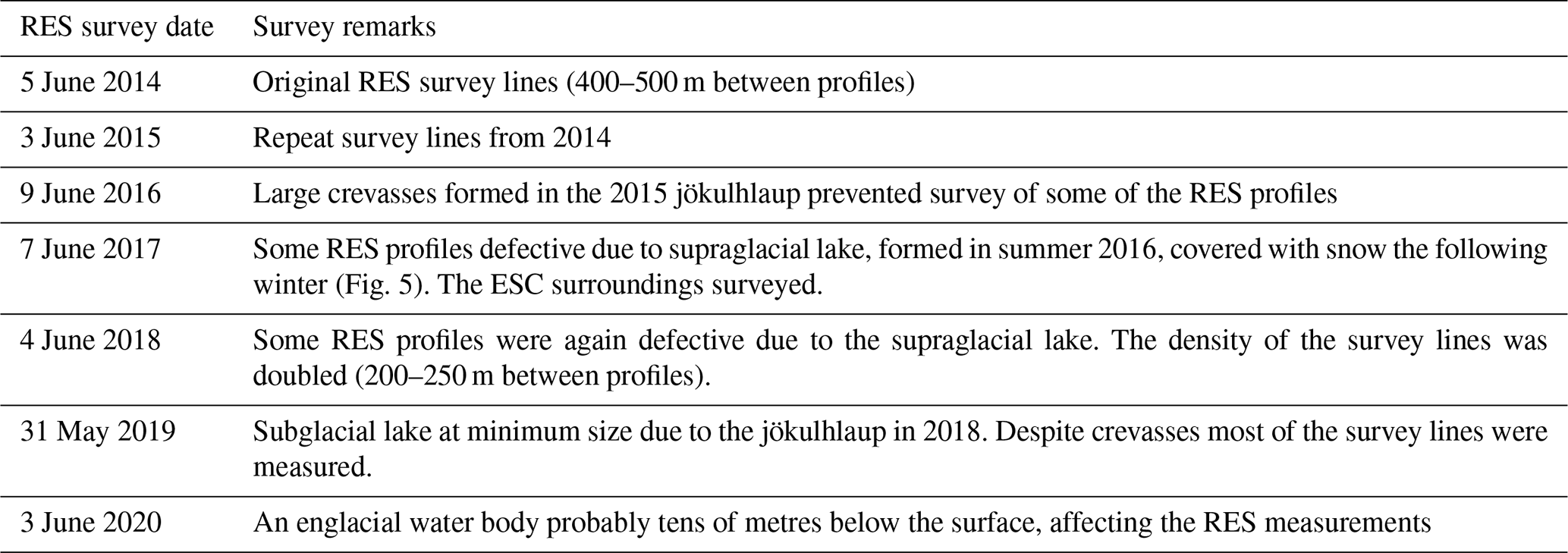
The RES data were obtained in early June or late May each year from 2014 to 2020 during the annual field trips of the Iceland Glaciological Society on Vatnajökull. The original profile grid over the ESC first measured in 2014 consists of two sets of parallel profiles, perpendicular to each other (Fig. 2b). This profile grid has since then been re-measured every year (Fig. 2–4) following a pre-planned track in the navigation instrument of the snowmobile. This typically results in < 10 m planar offsets between profiles from individual years, except when profiles are intersected by new crevasse formations. Dates and specific remarks concerning individual RES surveys are given in Table 1.

Figure 2(b) The initial RES survey route of the ESC (location in panel a) in 2014. The DEM presented with shaded relief and contour map (20 m interval) was obtained from TanDEM-X data acquired on 23 September 2015. (c–i) An example of 2D migrated RES profiles for part of this route (from A to B on b) for all survey years. The vertical exaggeration is 2-fold. On each profile, the traced bed reflection (both from ice–bedrock and ice–water interface) and surface elevation are shown along with same information from the survey in the preceding year.
The RES data were acquired using surveying practices developed previously in Iceland (e.g. Björnsson and Pálsson, 2020; Magnússon et al., 2021). The radar transmitter and receiver unit were placed on two sledges separated by distance, a (35–45 m varying between surveys), in a single line and towed along the ice surface using a snowmobile. The low radar frequency applied (5 MHz centre frequency) generally secures clear backscatter from the glacier bed beneath 200–700 m of temperate ice found at the ESC and nearby. During a RES survey, the radar transmits a pulse, which travels as a direct wave along the glacier surface between transmitter and receiver triggering the recording of the receiver (developed by Blue System Integration Ltd.; see Mingo and Flowers, 2010), as well as penetrating into the glacier. The penetrated signal is backscattered from englacial reflectors or the bed up to the receiver at the surface, which records the strength of both the direct and backscattered signal. The signal strength is recorded as a function of detection time relative to the triggering by the direct wave and adding to it the travelling time of the direct wave between transmitter and receiver (using 3.0×10⁸ m s−1 as the speed of the radar wave in air), which yields the two-way travel time of the backscattered signals. Each recording corresponds to 256 or 512 RES measurements stacked to increase signal-to-noise ratio. The sounding plus processing time of the stacked measurements of each recording is ∼ 1 s. The strong direct wave from the transmitter is estimated as the average waveform measured with the RES over several-kilometre-long segments. This is then subsequently subtracted from the corresponding RES recordings. The remaining backscatter is amplified as a function of travel time in order to have the backscatter strength roughly independent of the reflectors depth.
The snowmobile towing the radar was equipped with a Differential Global Navigation Satellite System (DGNSS) receiver. A centre position, M, between transmitter and receiver is assigned to each RES recording. It is derived from the GNSS timestamp obtained by the receiver unit for each RES sounding, and the corresponding position of the DGNSS on the snowmobile projected back along the DGNSS profile by a distance corresponding to half the antenna separation () plus b, the distance from the RES receiver sledge to the snowmobile (∼ 20 m). Both a and b were obtained with a tape measure for each survey and assumed fixed for each survey date. When surveying profiles without taking sharp turns, the horizontal accuracy of M is expected to be < 3 m, but errors are mainly due to variation in distance to the snowmobile, inexact timing of each RES survey (due to slightly varying sounding and processing time) and the towed sledges not always accurately following the path of the snowmobile. The vertical accuracy is < 0.5 m.
The obtained RES recordings along with M for each recording and corresponding transmitter and receiver 3D positions ( behind and in front of M, respectively, along the DGNSS profile) were used as input into 2D Kirchhoff migration (e.g. Schneider, 1978), programmed in MATLAB (®MathWorks). The migration was carried out assuming a radar signal propagation velocity through the glacier (cgl) of 1.68×10⁸ m s−1 (corresponding to cgl for dry ice with a density of 920 kg m−3 (e.g. Robin et al., 1969); the choice of cgl and validation from borehole survey is discussed in Sect. 4.1.3) and a 500 m radar beam width illuminating the glacier bed. This results in profile images as shown in Fig. 2. The horizontal and vertical resolution of these images is 5 and 1 m, respectively. This corresponds roughly to the horizontal sampling density when measuring with a ∼ 1 s interval at ∼ 20 km h−1 and an 80 MHz vertical sampling rate (in 2014–2017; it is 120 MHz for an upgraded receiver unit used in 2018–2020).
Backscatter from the glacier bed, which at this stage can be both ice–bedrock and ice–water interfaces, is usually recognized as the strongest continuous reflections in the 2D migrated amplitude images. The next steps including reflection tracing and subsampling of traced reflections from a 5 m interval to a 20 m interval with filtering and masking of traced reflections near sharp turns in profiles are the same as in Magnússon et al. (2021).
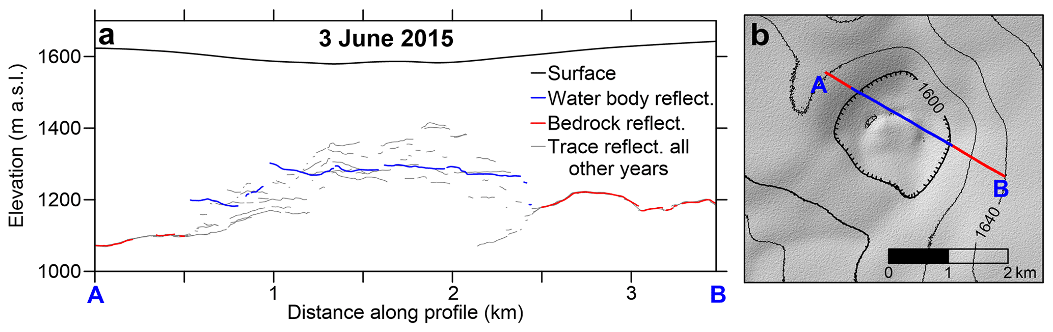
Figure 3(a) The traced reflections in 2015 (blue and red) for the same section of the RES survey route as in Fig. 2 compared with traced reflections of all other years (grey) from this profile section. This is used to classify traced reflections in 2015 as reflections from the roof of a water body (blue) and bedrock (red). The vertical exaggeration is 2-fold. (b) The corresponding classification for 2015 posted on a TanDEM-X DEM in September 2015.
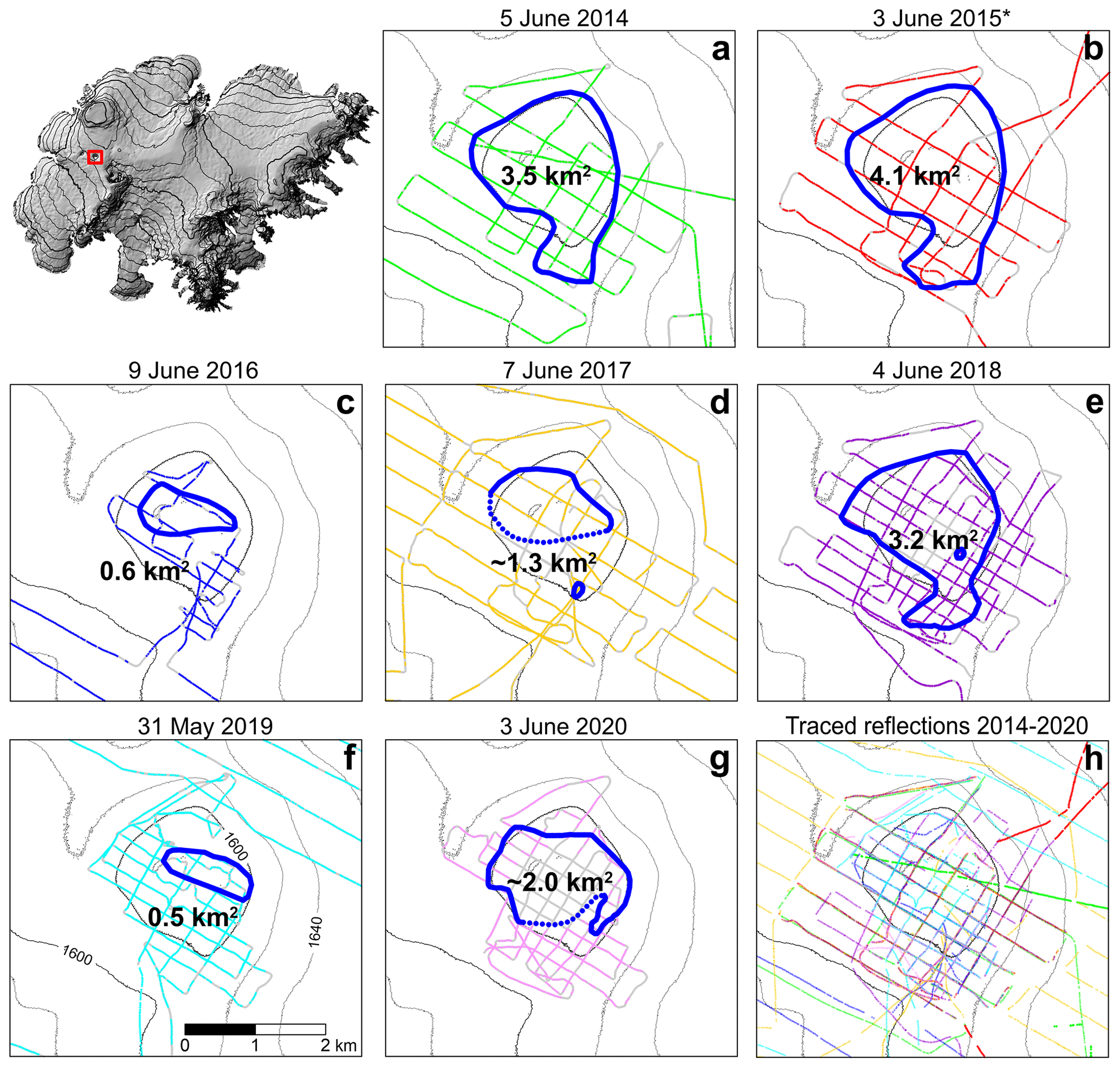
Figure 4(a–g) Traced bed reflections (both ice–water and ice–bedrock reflections) for the RES surveys in 2014–2020. Locations of traced reflections of each survey are displayed in different colours on top of the survey route of each year (shown as grey lines). The contour map shows the surface elevation in September 2015 (TanDEM-X). Polygons (blue line) and numbers indicate derived margin and area of the subglacial lake for the corresponding year. Poorly constrained sections of the lake margin are shown with a dotted line. Locations of all traced reflections with corresponding colour-coding are shown in panel (h). * Note that in panel (b) one profile, surveyed by driving from the cauldron's centre out of the study area towards northeast, was acquired in February 2015. It was only used to approximate the position of the lake margin in spring 2014 and 2015 and for tracing the bedrock reflection outside the lake.
2.2 Outlining the lake margin
At this stage, both the repeated migrated RES profiles as well as traced reflections were projected to a length axis common with the axis of the 2014 survey (the 2018 survey for the new profiles measured since 2018) to allow direct comparison. A slight difference in integrated length along profiles, due to a slight difference profile location between years, can otherwise obscure comparison between profiles. The projection onto a common length axis was only done for segments where the repeated profiles are < 50 m from the original profile. At locations where this deviation was 15–50 m it was considered whether differences in traced reflections were related to a mismatch between profile locations. The traced reflections were first compared in areas at or outside the rim of the ESC, undoubtedly showing a fixed bedrock surface for all surveys. The median elevation difference for the traced reflection in these areas, when compared to the master (2014), was used to bias-correct individual surveys in 2015–2020 towards the master, always resulting in < 2.5 m vertical shift (in 2018 and later, the shift is obtained from comparison with an interpolated bedrock DEM based on surveys from previous years). At this stage, the comparison of the profiles (Figs. 2–3) reveals areas for which the elevation of the traced reflections (median corrected in 2015–2020) is unchanged at the temporal minimum, between two or more survey dates, indicating reflections from bedrock for corresponding surveys. The comparison also reveals areas where the traced reflection of a given survey is clearly above the traced reflection of another, designating a reflection from an elevated ice–water interface. This helps identify the parts of a profile that are reflections from the lake roof (Fig. 3), which for the ESC is not at all revealed by a flat reflective surface. It also reveals that the edge of the lake is commonly characterized by relatively steep side walls, which further helps pinpointing the lake edge where repeated reflections from the bedrock were not obtained, as in 2016 and 2019 when the lake area was at its smallest. The lake margin was then approximated in between the RES profiles to obtain the lake outlines and area (Fig. 4). Some of the RES profiles in 2014 and 2015 did not fully span the areal extent of the lake. The lowering during the 2015 jökulhlaup (see Sect. 2.4) was therefore used to further guide the approximation of the 2015 lake margin where RES observations on the lake edge are not available. The obtained 2015 coverage and observed advance of the margin in 2014–2015 from the RES profiles were considered when approximating the 2014 lake margin. The outlines of the lake margin in 2016–2020 were, however, obtained from the RES data alone by manually drawing lines between obtained lake margin positions in profiles. For some years, a part of the lake margin is rather subjectively drawn. This is particularly the case for the south part of the lake margin in 2017, which should only be considered as a rough estimate (dotted line in Fig. 4d) since this part of the lake margin was beneath the snow-covered supraglacial lake (Fig. 5), which obstructed the RES signal obtained in this part of the cauldron. In 2018, the supraglacial lake was smaller and the margin of the subglacial lake had advanced beyond the extent of the supraglacial lake; hence the supraglacial lake did not obscure the detection of the subglacial lake margin. Similar defects in the 2020 RES data (Fig. 2i), likely caused by englacial water bodies, made it impossible to detect part of the southern lake margin. The approximated margin in 2020 (dotted line in Fig. 4g) is, however, constrained by traced reflections from bedrock a short distance south of the drawn margin; hence the lake area in 2020 cannot be much larger than the estimate presented here. Based on the above, we expect the uncertainty of the lake area to be ∼ 0.1 km2 for all years except in 2017 and 2020 when we estimate the uncertainty as ∼ 0.3 and ∼ 0.2 km2, respectively.
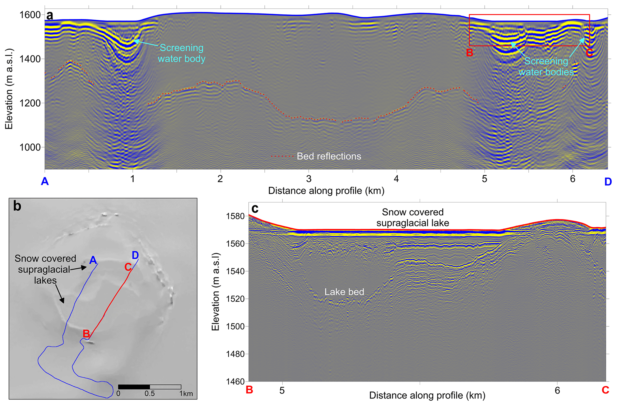
Figure 5(a) The low-frequency (5 MHz) RES survey (2D migrated) on 7 June 2017 from location A to D (location shown in panel b) revealing features which induce ringing in the received radar reflections, completely screening reflections from the glacier bed (traced reflections indicated with a red dotted line). The flat glacier surface above these features along with the Landsat-8 optical image in August 2017 (b) clearly reveals these features as snow-covered supraglacial lakes. RES survey on 8 June 2017 with 50 MHz Malå radar (c) along subsection B to C (location shown in panel b) repeating the low-frequency survey (corresponding part of the low-frequency RES profile is indicated with red box in panel a) further confirms this. Note that the elevation projection for panel (c) is carried out using m s−1. The propagation velocity through the media above the supraglacial lakebed is much lower; hence the depth of the lake as indicated in panel (c) is overestimated. The vertical exaggeration is 2.5-fold and 5-fold in panels (a) and (c), respectively.
2.3 Creation of bedrock DEM and lake thickness maps
The records of traced reflections were split in two groups, using the lake outlines derived above: (i) reflections from bedrock and (ii) reflections from the roof of the subglacial lake. The former data group was merged into a single data set. This includes data from profiles obtained in the vicinity of the ESC outside the area of repeated RES survey (mostly in 2017 and 2019; see Fig. 4d and f). The traced bedrock reflections display good coverage across the bedrock beneath the cauldrons except where the lake was present for all surveys (Fig. 4). In addition, the bedrock elevation beneath the cauldrons has been measured directly through two boreholes (Gaidos et al., 2020), which were located within the RES data gap. From the bedrock record, including borehole measurements, a bedrock DEM (Fig. 6a) with 20 m × 20 m cell size has been constructed using the kriging interpolation method (processed using Surfer 13 © Golden Software LLC).
The filtered and revised records of traced reflections from a given year obtained within the corresponding lake margin were assumed to originate from a lake roof. The lake roof records of individual survey epochs were then differenced from the interpolated bedrock DEM to obtain lake thickness for each data point. The lake outlines were converted to input data points (with 20 m interval) with a prescribed lake thickness of zero before interpolating each lake thickness map (using the kriging function in Surfer 13) for each year (Fig. 6). At a few locations, minor adjustments of the interpolated maps were made because of disagreement between crossing profiles. This only occurred in areas of very steep topography in the lake roof where 2D migration tends to fail, particularly for profiles driven perpendicular to the slope direction of the underlying lake roof (see Sect. 4.1.2). In such cases, the manual adjustment favoured data from profiles which were more parallel to the roof's slope direction. Lake volumes (Fig. 6) were obtained by integrating the individual thickness maps. In 2020, only the area could be obtained from the RES data; the lake topography was only partly surveyed (Fig. 6h) due to strong internal reflections (see Sect. 2.1), prohibiting direct integration of the lake volume. In this case, the volume of the lake was estimated assuming a linear relation between the lake area and volume using the values obtained in 2014–2019 (Fig. 6i).
2.4 Elevation changes and released volume of water during jökulhlaups in 2015 and 2018
The DEMs used to measure the surface lowering of the ESC during the jökulhlaup in 2015 were deduced from interferometric synthetic aperture radar (InSAR) data acquired during the TanDEM-X satellite mission on 23 September and 10 October, a few days before and approximately a week after the jökulhlaup. The DEMs are processed by extracting the topographic information from the InSAR data in the same manner as described by Rossi et al. (2012). Differencing the two DEMs reveals the area affected by the depletion of the subglacial lake as a clear anomaly, outlined in Fig. 7a, as well as surface lowering above the flood route from the lake south of the cauldron. The DEM difference was corrected for near-homogenous surface elevation changes between the two dates, unrelated to the jökulhlaup, and for slowly varying elevation errors in the DEMs, e.g. caused by different penetration of the radar signal into the glacier surface at the two dates (Rossi et al., 2016). Around the outlined anomaly, excluding the flood route, a ∼ 500 m wide reference area was defined, where the elevation changes due to the 2015 jökulhlaup are expected to be insignificant (within few decimetres). The least-squares method was used to fit a linear plane through the obtained elevation difference within this reference area, which we then subtracted from the elevation difference between the two DEMs.
The DEM prior to the jökulhlaup in early August 2018 was constructed from a DEM obtained as part of the ArcticDEM project (Porter at al., 2018) in August 2017, corrected with the DGNSS profiles acquired on 4 June during the 2018 RES survey of the ESC (Fig. 4e). The elevation changes, during the jökulhlaup, were obtained by comparing this DEM with the airborne radar altimetry profiles with an approximate accuracy of 1–2 m (for more details, see Gudmundsson et al., 2016), acquired on 9 August, a few days after the jökulhlaup (Fig. 7d). The difference between the DEM and the radar-altimetry profiles was interpolated with kriging to obtain a map of elevation changes during the jökulhlaup. To compensate for surface elevation changes from 4 June and 9 August, unrelated to the jökulhlaup, a linear plane was again subtracted from the obtained map of elevation changes. The linear plane was obtained in the same way as for the jökulhlaup in 2015, except the westernmost part of the reference area from 2015 was excluded, due to elevation changes related to a jökulhlaup from the WSC, which occurred at the same time as the flood from the ESC in 2018.
To obtain a measurement of water volume released during the jökulhlaups, the elevation changes were integrated within the outlined area of lowering due to the depletion of the lake. The area where this lowering was more than a few decimetres is quite distinctive in the 2015 elevation change map. The less accurate elevation change map during the 2018 jökulhlaup, due to the sparse altimetry data after the jökulhlaup (profile location shown in Fig. 7d) and a larger time gap between the pre-jökulhlaup DEM and the jökulhlaup (∼ 2 months compared to only few days in 2015), made it difficult to directly outline the area of lowering in 2018. It was therefore assumed that the lowering area was the same as in 2015 (dashed line in Fig. 7c). The integrated volume change within this area was 280 ± 5 GL for the jökulhlaup in 2015 and 180 ± 18 GL in 2018. The uncertainty corresponds to a possible bias of 0.25 and 1.0 m for the elevation change maps for in 2015 and 2018, respectively, for the area of integration. It is approximated from the variations in obtained elevation difference outside the area of integration. The volume change during the jökulhlaup, corresponding to the water released from the lake, consists of both the volume integrated from the surface elevation change detectable from the DEMs and the formation of crevasses, which can penetrate deep into the glacier and are not represented in the post-jökulhlaup elevation data. The crevasse field surrounding the ESC after the jökulhlaup in 2015 formed an ∼ 8 km long arc. Assuming that the cumulative width of the crevasses across the 300–400 m wide crevasse field is 100 m at the surface and that this width decreases linearly with depth to 0 m at 100 m depth results in a volume of 40 GL (Guðmundsson et al., 2018). In 2018, the crevasse field had a similar area (shorter arc but wider) resulting in the same crevasse volume estimate. The uncertainties of these estimates are assumed to be rather high, or 50% of the derived values. Combined with the uncertainty of volumes from the DEM difference results in 20 and 30 GL uncertainty in the lake release volume in the 2015 and 2018 jökulhlaups, respectively.
2.5 Validation of the RES results
We did not attempt to estimate the uncertainty of the lake volumes derived from the RES data directly. Various factors, which are difficult to quantify, can contribute to this uncertainty, and the dependency between different uncertainty factors is unclear and therefore problematic to combine into a single value (discussed further in Sect. 4.1). Instead, the lake volumes derived from the RES data were validated by comparing them with the volume of water released during jökulhlaups, obtained from measured surface lowering (Figs. 7–8). The results of the validation are described in Sect. 3.1.
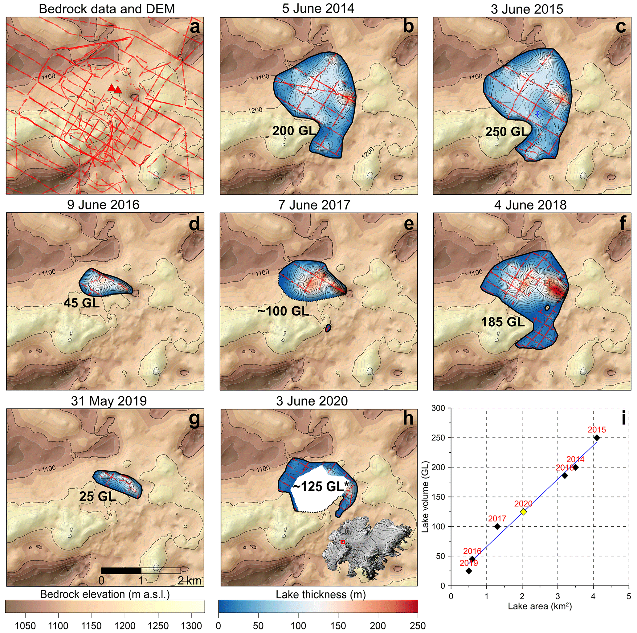
Figure 6(a) The location of traced reflections classified as reflections from bedrock (red lines) in the combined 2014–2020 RES record along with elevation of bedrock measured through boreholes (red triangles) used to interpolate a DEM of the bedrock beneath the ESC and near vicinity (area shown with red box in inset image on h). This DEM, represented with the elevation contour map (20 m contour interval), is shown in the background of (a)–(h). (b–h) Maps of lake thickness along with the location of traced reflections classified as reflections from the lake roof (red lines), used to interpolate the lake thickness map for each survey. Lake volumes integrated from the lake thickness maps are displayed in GL (106 m3). (i) The lake volume posted as a function of lake area (in 2014–2019; black diamonds), which constrains a linear relation (blue line) used to estimate the lake volume in 2020 (value marked with * in panel h and yellow diamond in panel i), when the lake thickness map had a large data gap (white area).
3.1 Lake area and volume
The evolution of the lake area inferred from the RES surveys in 2014–2020 is shown in Fig. 4. The minimum area of 0.5–0.6 km2 was observed less than a year after the 2015 and 2018 jökulhlaups, while the maximum of 4.1 km2 was observed in June 2015, ∼ 4 months prior to a jökulhlaup. At the time of this observed maximum lake area in 2015, almost 5 years had passed from the previous jökulhlaup from the ESC in July 2010 (Guðmundsson et al., 2018). In comparison, the lake had expanded to 3.2 km2 in June 2018, 2 months prior to the 2018 jökulhlaup.
The lake development in terms of volume and shape is shown in Fig. 6. The strong positive linear relation between the area and volume of the subglacial lake is demonstrated in Fig. 6i. The variation of lake volume obtained with RES and the estimated volumes of water released during the jökulhlaups extracted from surface elevation changes (Fig. 7c–d) are displayed in Fig. 8. The RES surveys indicate lake volumes < 50 GL in 2016 and 2019, less than a year after jökulhlaups, which strongly suggests that the lake drained completely or was reduced to an insignificant volume in the preceding jökulhlaups. The lake volume prior to each jökulhlaup and the released volumes during them should therefore be comparable, further justifying the validation of the RES results (Sect. 2.5). A maximum volume of 250 GL is derived for June 2015 compared with a volume of 320 ± 20 GL released during the jökulhlaup ∼ 4 months later. The survey in June 2018 yields a volume of 185 GL, while the released volume in August the same year was 220 ± 30 GL. At the onset of the 2018 jökulhlaup, the water volume in the lake had already been estimated to be 180 GL, using the available RES record from the ESC in 2014–2018 (Guðmundsson et al., 2018). Some of the difference between the volumes obtained from RES in June 2015 and 2018 and from surface lowering during jökulhlaups 2–4 months later is likely explained by more rapid lake growth during summers compared to winter due to inflow of meltwater from the glacier surface. With this in mind, the errors in RES volumes were probably < 20 % and < 10 % in 2015 and 2018, respectively. The development of the lake volume in 2010–2020, assuming it drained completely in the jökulhlaup in July 2010, mimics a sawtooth curve (Fig. 8a) with an approximately fixed filling rate of ∼ 60 GL a−1 between jökulhlaups (Fig. 8b). The values in 2014 and 2015 are slightly offset from this trend, possibly due to a less dense profile network then than for later surveys. If the RES surveys of 2014 and 2015 are excluded, the filling rate between jökulhlaups is ∼ 65 GL a−1. Given how well the combined record of lake volumes from RES and observed surface lowering fit a linear relation with time elapsed since the previous jökulhlaup (Fig. 8b), we expect the uncertainties in the RES volumes to be 10 %–20 %, as in 2015 and 2018, except when the lake is small (< 100 GL) and therefore not posing significant hazard (uncertainties > 10 GL should be expected with this approach). By measuring a denser RES profile network as done since 2018, the uncertainty has probably decreased to ∼ 10 % for favourable surveying conditions.
It is worth noting how poorly the measured surface elevation at the ESC centre correlates with the lake volume beneath the cauldron (Fig. 8). This indicates the governing role of ice dynamics for filling up the cauldron surface depression, while the contribution of water accumulation in the lake to surface elevation changes is small in comparison; large proportions of the accumulated water simply replace ice melted beneath the cauldron.

Figure 7(a–b) The ESC lake thickness maps 4 and 2 months before the jökulhlaups in 2015 and 2018, respectively (from Fig. 6c and f). (c–d) Maps of glacier surface lowering during these jökulhlaups. The dashed red line indicates the area of integrated surface lowering corresponding to the area of notable surface lowering during the 2015 jökulhlaup. The grey lines in panel (d) indicate the locations of radar altimetry profiles surveyed from an aeroplane on 9 August 2018, a week after the jökulhlaup. The total volume of the lake integrated from the lake thickness maps (a–b) and the released volume integrated from the surface lowering during jökulhlaup adding estimated volume of crevasses (c–d) are displayed in GL (106 m3). (e–f) The difference between lake thickness obtained by RES, in 2015 and 2018, and the lowering during the following jökulhlaup. Polygons filled with diagonal crosses indicate the areas of large crevasses formed during the jökulhlaups as outlined from Fig. 1c–d. The contour maps indicate surface elevation (20 m contour interval) from TanDEM-X on 10 October 2015 (e) and from the altimetry profiles on 9 August 2018 (f) as explained in Sect. 2.4. The green triangle in panels (a)–(f) indicates location of a GNSS station operating during both jökulhlaups.
3.2 Lake shape
A striking feature in the lake shape for all observations is steep side walls, clearly represented in Fig. 9a–b, typically exceeding 45∘ slopes and sometimes even 60∘. Despite the apparent linear relation between the lake volume and area (Fig. 6i), the overall shape of the lake varies substantially during the study period. In 2014 and 2015, before the jökulhlaup in autumn 2015, the water was distributed much more evenly over the lake area than in 2018. Even though the lake volume and area in 2018 were close to the values obtained for 2014, the lake water was more concentrated close to the ESC centre with the maximum lake thickness above the crater-shaped bed depression beneath the eastern side of the ESC (Figs. 6–8), ∼ 0.5 km east of the boreholes (Figs. 6a and 7a). The shape of the subglacial lake margin also differed between 2015 and 2018. The steep side walls still surrounded the main bulk of the lake in 2018. However, the lake generally extended a few hundred metres outside these walls with an area of 10–30 m thick water layer (see Fig. 6f and left side of Fig. 9b). This clear difference in the lake shape before the 2015 and 2018 jökulhlaups is also apparent in the lowering during these jökulhlaups (Fig. 7c–d). Despite greater lake thickness beneath the ESC centre in 2018 (Figs. 9a–b and 7a–b) the surface elevation was similar to that in 2015 (Figs. 9a–b and 8a). Prior to the 2018 jökulhlaup, the ice above the lake was, however, relatively thin; in 2017 the minimum ice thickness was only ∼ 150 m, but it had increased to ∼ 180 m in 2018. Prior to the 2015 jökulhlaup, when the lake water was more evenly distributed, the corresponding values were ∼ 260 and ∼ 280 m in 2014 and 2015, respectively. The outward migration of the lake margin, typically by 50–150 m, appears as outward propagation of the steep ice walls that defined the lake margin. The steep side walls also seem to characterize the lake margin in 2017, but this was quite different in 2018. Due to the formation of previously mentioned 10–30 m thick water layer surrounding the steep lake walls in 2018, the lake margin typically advanced by 100–1000 m (Fig. 6e–f).

Figure 8(a) The development of the lake volume (left y axis) in GL (106 m3) beneath the ESC in 2010 to 2020 obtained from the RES data (black and yellow diamonds) and derived surface lowering during jökulhlaups adding estimated volume of crevasses (cyan diamonds). The latter includes estimated uncertainty. It is assumed that the lake drained completely during the jökulhlaups in 2010, 2015 and 2018. Red dots show the measured elevation (right y axis) of the ESC centre from radar altimetry and GNSS surface profiling (Gudmundsson and Högnadóttir, 2021). (b) The same lake development and cauldron centre elevation as a function of time elapsed since the previous jökulhlaup. The solid red line shows a linear fit through origin (zero volume at time zero) for the lake development; the dashed red line excludes the RES surveys in 2014–2015.
3.3 Lake topography vs. lowering during jökulhlaups in 2015 and 2018
When comparing the obtained lake thickness map prior to jökulhlaups and the subsequent lowering (Figs. 7 and 9), the surveyed shape of the lake and the lowering shows strong similarities. The lowering appears like a spatially filtered version of the lake thickness shape, with the maxima at approximately the same location and substantial lowering (> 5 m) extending typically 200–500 m outside the lake margin as obtained from the RES survey (Fig. 7). Figure 7e–f shows the derived difference between the lake thickness in spring 2015 and 2018 and the lowering during the jökulhlaups a few months later when the lake most likely drained completely or was reduced to an insignificant volume (Fig. 8). This difference, therefore, indicates where the ice became thinner or thicker during and shortly after the jökulhlaups, as well as the outlines of excessively crevassed areas formed during these floods. The main thinning areas as well as the main crevasse areas are located at or outside the main ice walls of the lake. In 2015, this coincides with the lake margin but not in 2018 as mentioned above. The main exception from this is the derived thinning in the northern part of the ESC in 2015, which extends significantly into the cauldron. The lake thickness in this area is, however, not covered with direct RES observation (red profiles in Fig. 7a); hence, the apparent thinning may be an artefact, as the relatively sparse RES profiling did not capture the amount of water stored in this area prior to the 2015 jökulhlaup. This further suggests that the true lake volumes in 2014 and 2015, based on the RES data, are underestimated. The thickening areas approximately correspond to the lake roof within the ice wall of the lake and the surrounding crevasse fields formed during the jökulhlaups. The thickening in 2015 was widespread, typically less than 40 m, and at the centre of the cauldron our estimation suggests thinning, but that may be due to scarce bedrock data at this location (Fig. 6a). In 2018, the thickening was much more localized and exceeded 40 m for substantial part of the area where the ice grew thicker. In both jökulhlaups, the area above the crater-like bed depression beneath at the eastern side of the cauldron yielded by far the greatest thickening. In 2015, the derived thickening at this location was up to 110 m, while in 2018 it was up to 170 m.
4.1 The limitations of the RES survey for quantifying the lake development
There are various uncertain factors, which may contribute to errors in the results derived from the RES data. This includes uncertain value of cgl, limitations of the 2D migration applied and interpolation errors due to sparse data coverage for obtaining both the bedrock DEM and the lake thickness maps. Each of these factors may produce systematic errors, which can lead to an either underestimated or overestimated lake volume. Below we further discuss these limitations and conclude with remarks on how these errors relate to the validation (see Sect. 2.5 and 3.1).
4.1.1 RES data gaps
The bedrock area concealed by the subglacial lake in all RES surveys is 0.35 km2 or ∼ 10 % of the lake area in 2018 and less in 2015. The centre of this gap in the RES bedrock observations is constrained with direct observations of bedrock elevation through boreholes. The contribution of this bedrock data gap to errors in the lake volume estimates is therefore expected to be small, except when the lake is small and mostly within the area of limited bedrock data. At other locations in the RES profile network, reflections from the bedrock have generally been traced at some time point, meaning that for most observations of roof elevation there is also an observation of the bedrock elevation at the same location. Interpolation errors outside the bedrock RES data gap, contributing to errors in the lake volume estimate, are therefore mostly related to the interpolation of the lake thickness and not the bedrock elevation.
Supraglacial lakes and englacial water bodies, further discussed below, produce gaps in the data used to interpolate lake thickness maps for some years. For this reason, we consider the uncertainties of the lake volumes obtained in 2017 and 2020 at the upper limit (∼ 20 %) of the uncertainty range obtained from the validation (Sect. 2.5) – in 2017 mostly due to uncertain location of the lake margin and in 2020 due to possible deviations from the obtained linear relation between lake volume and area (Fig. 6i). The survey in 2018 is also affected by similar data gaps. The lake margin is, however, fairly well constrained, and only ∼ 15 % (∼ 0.5 km2) of the lake area (3.2 km2 in total) is affected by these data gaps. Interpolation errors in the lake thickness maps are probably resulting in larger lake volume errors in 2014 and 2015 when the distance between RES profiles was 400–500 m, compared with 200–250 m in 2018 and later.
4.1.2 Limitations of the 2D migration
In most glaciological applications, only 2D migration of RES data is possible for locating radar reflections, but this requires the assumption that all radar reflections originate from directly beneath the survey profile. This is often not the case beneath glaciers that flow over volcanic regions, where the subglacial topography is particularly complex. The associated errors in reflection location are most pronounced when profiles are surveyed perpendicular to slope direction of the reflective surface (e.g. Lapazaran et al., 2016). If the traced reflective bedrock surface is not directly beneath the RES profile but across the track, the obtained ice thickness is underestimated and the mapped surface below the profile is estimated to be too high. This has been shown using an experiment comparing 2D and 3D migrated RES data obtained above steep bedrock beneath Gulkana Glacier, Alaska, which clearly indicated such an overestimate in bed elevation from the 2D migrated data (Moran et al., 2000). Similar results were obtained in a recent study on Mýrdalsjökull ice cap in southern Iceland (Magnússon et al., 2021) in topographic settings similar to the ESC, using the same radar system as applied here. In that study, traced bed reflections from 2D migrated profiles were found to be on average 10 m higher than the bedrock DEM obtained from 3D migrated data. The same study showed that when using the 2D migrated data (200 m profile separation) interpolation errors in a bedrock DEM deduced from it were insignificant in comparison to the errors caused by the 2D migration. In the study presented here, where crevasses and the size of the study area do not allow a safe acquisition of data for 3D migration with a reasonable effort, we may expect the 2D migration to introduce a similar bias. This, however, applies to both the reflections from the bedrock and the lake roof shifting both surfaces upwards; hence the effects of this may to some extent be cancelled out, when estimating lake thickness and volume. The resulting bias in the surveyed lake roof elevation should, however, vary between observations and be most prominent when the topography of the lake roof was most uneven in 2017–2018. Assuming that the error in lake volume due the shortcoming of the 2D migration can typically correspond to ∼ 5 m, the average offset in lake thickness would correspond to ∼ 10 % error in lake volume.
The RES profiles do not necessarily pass directly above subglacial topographic peaks, which may cause some further distortion in the lake thickness maps and bedrock DEM. In steep areas, these topographic peaks are, however, represented as somewhat lower peaks at the RES profiles close to the actual peaks due to the cross-track reflection explained above. The height of topographic peaks in the lake may therefore be slightly underestimated, and their exact planar position is likely somewhere between survey profiles but not directly beneath them as shown in Fig. 6b–h. The denser RES profile network surveyed since 2018 should reduce these errors.
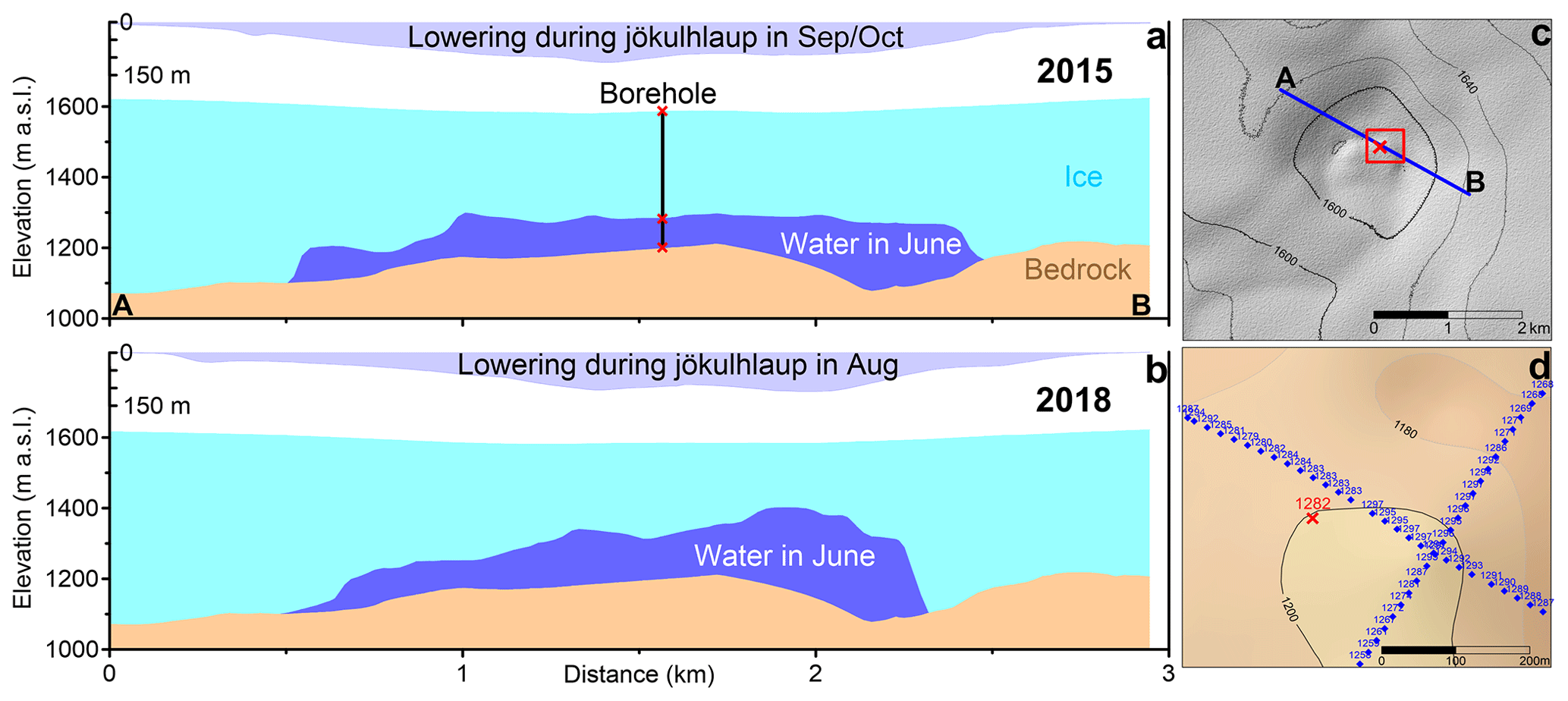
Figure 9(a–b) Cross section over the centre part of the ESC from location A to B (shown in panel c) revealing bedrock, lake and ice thickness, 4 and 2 months before the jökulhlaups in 2015 (a) and 2018 (b), respectively. The lowering along this cross section during the subsequent jökulhlaup (derived from Fig. 7) is shown in the upper part of each panel. Note that the y axis is without vertical exaggeration. (d) Comparison of lake roof elevation measured with RES, 3 June 2015 (blue numbers and diamonds), and through boreholes, 7 June 2015 (red number and x). The borehole location relative to the cross-section A to B is shown in panels (a) and (c). Red box in panel (c) indicates the area shown in panel (d).
4.1.3 Errors in radio wave velocity (cgl)
We have a single borehole survey (Fig. 9d), which can be used to validate cgl used in the RES processing. The difference between the lake roof elevation at the borehole and nearest point on the profiles is 1 m when using m s−1. Taking into account the mismatch in profile and borehole location (∼ 50 m) and the spatial variability in lake roof elevation from the RES data, it is unlikely that the actual difference between the lake roof elevation at the two locations exceeds 10 m, setting a boundary on the cgl uncertainty, resulting in m s−1. Further, cgl at this specific location and time may deviate from the average value of cgl in the survey area. We consider it unlikely that cgl exceeds m s−1, corresponding to the propagation velocity through dry ice with density 900 kg m−3 (Robin et al., 1969). The water content in the temperate ice can, however, reduce cgl significantly (e.g. Smith and Evans, 1972), even below 1.60×10⁸ m s−1 (e.g. Murray et al., 2000). Given the value obtained at the borehole, we consider it unlikely that the average value of cgl in the survey area is below 1.60×10⁸ m s−1. If we assume that the spatially averaged value of cgl is approximately the same for all surveys (as suggested by the good agreement of repeated bedrock profile sections), the error in cgl should shift both the lake roof and the bedrock in the same direction proportional to the ice thickness (without a lake above in the case of bedrock) except for the relatively small part of the bedrock DEM constrained by borehole measurements (Fig. 6a). Consequently, the error in lake thickness as well as volume due to erroneous cgl should be proportional to the error in the applied value of cgl. If the applied cgl is too high, the lake thickness is overestimated, and it is underestimated if the applied cgl is too low. For example, if the true value of cgl is 1.60×10⁸ m s−1 when the value of 1.68×10⁸ m s−1 is used, the lake volume would be overestimated by ∼ 5 %. Considering that the upper limit of cgl is 1.70×10⁸ m s−1, a significant underestimate in lake thickness because of too low an applied value of cgl is unlikely. Some of the errors introduced by using value that is too high for cgl may be cancelled out by the 2D migration tending to shift reflective surfaces upwards as explained above. If the value applied for cgl is too low, the 2D migration may further exaggerate these errors.
Due to the temporary presence of supraglacial lakes within the ESC (Fig. 5) and englacial water bodies beneath it (Fig. 2i), the value of cgl may differ significantly between the bedrock and some lake measurements, leading to larger lake thickness errors at locations where such water bodies appeared. Supraglacial lakes sometimes form within the ESC, probably as a consequence of highly compressive strain rates at the cauldron centre sealing water routes from the glacier surface down to the subglacial lake, resulting in accumulation of surface meltwater within the cauldron. It is worth noting that it is possible to trace in 50 MHz radar data (Fig. 5c) a flat water table of an aquifer layer extending from and between the supraglacial lakes. The presence of a supraglacial lake both screens out reflections from the bed beneath the supraglacial lake and reduces cgl, due to increased water content in the media penetrated by the radar. This may affect the traced reflection in areas where the supraglacial lake is not deep enough to fully screen out reflections from the bed or due to high water content close to the glacier surface related to an aquifer layer. This effect was observed in the 2017 RES survey. Then bed reflections outside the subglacial lake, at the edge of the supraglacial lake, appeared up to 20 m below the bedrock elevation observed at same locations in 2019. The lower elevation of the 2017 reflection was attributed to a delay caused by the supraglacial lake and therefore not traced. Around 100 m farther away from the supraglacial lake in 2017, the RES surveys in 2017 and 2019 showed the bed reflections at approximately the same elevation, indicating that a delay caused by the aquifer layer extending from the lake in 2017 is insignificant or limited to the shore of the supraglacial lake. The delay caused by a shallow supraglacial lake may result in a 10–20 m overestimate in the depth of some of the traced reflections in 2017 and 2018 near the data gaps seen as grey (untraced) profiles near the ESC centre in Fig. 4d–e. This may contribute to a corresponding underestimate of the lake thickness for a minority of the traced reflections from the lake roof in 2017 and 2018. It is worth noting that the unusually undulating lake roof topography for the same years is likely to cause unusually high upward shift of the lake roof elevation through the previously described limitation of the 2D migration, contributing to an overestimate in lake thickness. It is not certain which of these two counteracting errors influence the derived lake volumes more in 2017 and 2018.
In 2020, englacial features obstruct reflection from the bed (Fig. 2i) in the same way as the supraglacial lakes in 2017 and 2018. There were no indications in 2020 of snow-covered supraglacial lakes, and these features appeared at greater depth than in 2017 and 2018; hence these artefacts in 2020 are attributed to an englacial water layer (sill). Such layers probably need to be several metres thick to produce similar artefacts to the supraglacial lakes, which was apparently the case for a large part of the ESC centre area in 2020. As a result, reflections from the lake roof could only be traced for a small part of the profiles crossing the subglacial lake. Fortunately, the lake margin could be mapped allowing an estimate of lake volume, due to the previously mentioned strong relation between the lake volume and area in 2014–2019 (Fig. 6i). When viewing the RES profiles for other years (Fig. 2), we typically see englacial features likely related to water bodies or layers too thin to screen reflections from the lake roof and the bedrock. There are even indications of such a layer near the centre of the RES profile in Fig. 2d corresponding to the time (2015) and the location where the lake roof elevation was directly measured through a borehole (Fig. 9d), showing matching lake roof elevation with m s−1. This indicates that despite likely existence of these englacial water bodies they are not causing an excessive delay and likely affecting all RES surveys in a similar manner in 2014–2019. Likely deviation of cgl in 2020, due to thick englacial water layers, does not affect the corresponding lake volume, as it was estimated using the derived lake area and not by integrating a lake thickness map.
The above discussion on likely errors in water volumes due to errors in the 2D migration (< 10 %) and wrong value of cgl (< 5 %, given that the temporal variability of cgl is small where lake roof/bed reflections could be detected) is in fair agreement with the independent validation (Sects. 2.5 and 3.1) yielding 10 %–20 % uncertainty in the lake volumes (for a lake > 100 GL) obtained from the RES, particularly if these errors counteract one another. Furthermore, interpolation errors likely added to the uncertainty of the result in the first years of our survey when the profile separation was ∼ 400 m, but by reducing profile separation down to ∼ 200 m the interpolation errors have likely become insignificant in comparison with the migration errors.
4.2 The shape of the subglacial lake and its evolution in 2014–2020
The repeated RES surveys in 2014–2020 yield new insight into the shape of the subglacial lake beneath the ESC and how it has evolved in recent years. The steep, almost step like, side walls (Figs. 2, 6 and 7) differ from the typical conceptual models of lakes beneath ice cauldrons (e.g. Björnsson, 1988; Einarsson et al., 2017) with the lakes drawn with smooth, approximately parabolic or elliptic, cross sections. It is also different in form from attempts to approximate the lake shape based on the difference between cauldron surface elevation shortly before and after a jökulhlaup (Einarsson et al., 2017). The observed step-like structures in the lake shape may be an indication of intensive melting at the lake roof and the upper part of the ice walls, with much lower melt rate on the lower part of the ice walls. The difference in lake shape before the 2015 and 2018 jökulhlaups (see Sect. 3.2) was at least partly caused by changes in the geothermal area below the ESC. Temperature profiles within the subglacial lakes beneath the Skaftá cauldrons have revealed temperatures of 3–5 ∘C that are mostly independent of lake depth, thus enabling effective convection to take place (Jóhannesson et al., 2007; unpublished data at the IMO). Chemical analyses of the water in the WSC lake revealed a component of geothermal fluid of deep origin at ∼ 300 ∘C (Jóhannesson et al., 2007). In 2016–2018 the main vents of the geothermal area, forming centres of strong convection plumes with peak basal melting directly above, were probably close to the two main maxima in lake thickness observed in all 3 years at approximately the same location (Fig. 6d–f). These maxima, indicating the locations where most ice had been replaced by meltwater since the 2015 jökulhlaup, were beneath the east side of the cauldron, above the west side of a sharp crater-like depression in the bedrock (Sect. 3.3) and ∼ 800 m farther west, close to the cauldron centre. The same maxima had started forming in 2019 (Fig. 6g) and at least the eastern one had continued growing in 2020 (Fig. 6h). During the period 2010–2015 these two vents in the geothermal system were probably not as powerful as in 2015–2018, explaining the large difference in minimum ice cover thickness for these two periods (260–280 m in 2014–2015 vs. 150–180 m in 2016–2018). A substantial part of the geothermal power in 2010–2015 was likely released by other parts of the geothermal area beneath the ESC, which typically are much weaker or dormant, explaining the relatively uniform lake thickness in 2014 and 2015. Such a temporal increase in geothermal activity in 2010–2015 probably occurred near the northernmost and southernmost part of the lake in 2014 and 2015. The observed lowering during the jökulhlaup from the ESC in 2010 and the evolution of the ESC since the mid 20th century (Gudmundsson et al., 2018) indicate that this behaviour in 2010–2015 was unusual for the geothermal area, and the activity in 2015–2018 resembles more the behaviour prior to 2010. Even though the distribution of the released geothermal energy was different for the two periods, the net power of the geothermal area was probably similar, as represented in a similar rate of water accumulation in the lake over time (Fig. 8b).
Despite the indication of changes in the geothermal area, it should be kept in mind that the lake accumulated water for 5 years before the jökulhlaup in 2015 compared with 3 years for the 2018 flood. Some of the difference in lake shape may be due to this. However, the thickening of the ice cover in 2017–2018 (∼ 30 m a−1 at the cauldron centre) and the outward migration of steep ice walls seem too slow to explain the different lake appearance in 2015 compared with 2018. The difference in lake shape may, however, have contributed to the earlier onset of the jökulhlaup in 2018. The shallow lake area outside the steep ice walls in 2018 may be an indication that the glacier outside the walls had started to float up as a consequence of high water pressure in the subglacial lake. This high subglacial water pressure likely extended somewhat away from the lake through connections in the subglacial drainage system outside of the lake. This may have contributed to the onset of a jökulhlaup 2 months later.
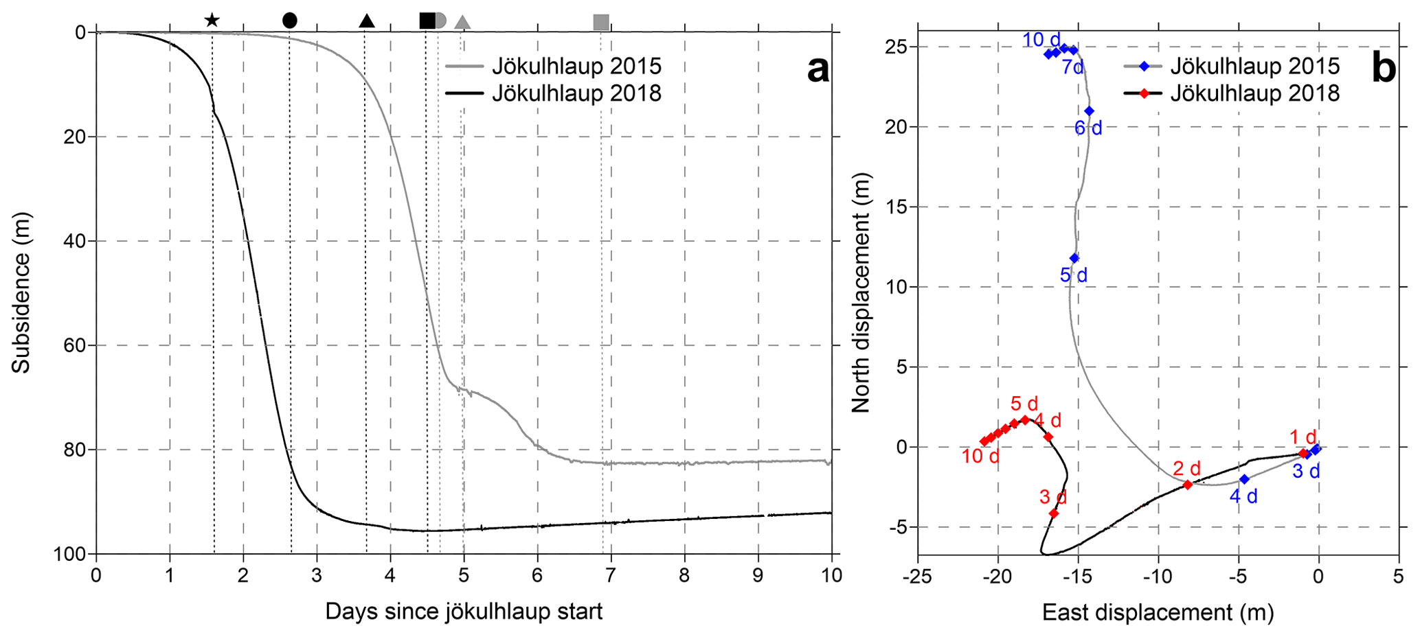
Figure 10(a) The subsidence of the GNSS station in the ESC (exact location shown in Fig. 7) during the jökulhlaups in 2015 (grey profile) and 2018 (black). The symbols (star, circles, triangles and squares) mark timestamps of events discussed in Sect. 4.3. (b) A planar view showing the horizontal track of the station during the jökulhlaup relative to its position at the onset of the jökulhlaup. Blue and red diamonds show positions of the station at 24 h intervals during the 2015 and 2018 jökulhlaups, respectively.
The RES surveys in 2014–2020 have revealed supraglacial lakes as temporal features sometimes forming in the ESC, and even though englacial water bodies and layers are generally found beneath the cauldron, it seems that in 2020 these features were more prominent than in other years. This highlights the temporal variability in the englacial and supraglacial hydrology at or beneath the ESC. As suggested by Gaidos et al. (2020), the englacial water bodies may play an important role in the triggering of jökulhlaups from the Skaftá cauldrons. A jökulhlaup from the WSC in 2015 was most likely triggered via the drilling of a borehole at the cauldron centre, which created a pressure connection between the subglacial lake and an englacial water body above it (Gaidos et al., 2020). Sudden drainage of supraglacial lakes down to the glacier bed (e.g. Das et al., 2008) also highlights these lakes as a potential trigger of jökulhlaups from subglacial lakes, which should be studied further.
4.3 The jökulhlaups in 2015 and 2018
The jökulhlaup in 2015 has been the subject of recently published studies. Ultee et al. (2020) estimated the tensile strength of the glacial ice from the location of crevasse fields formed during the jökulhlaup, and Eibl et al. (2020) studied the seismic tremor related to the jökulhlaup and the potential of using seismic array measurements of the tremor for early warning of subglacial floods. The jökulhlaup in 2018 has not yet received similar attention. The GNSS station, operated by IMO, was running at approximately the same location near the centre of the ESC (Fig. 7) during both jökulhlaups.
During the weeks prior to the jökulhlaup the station had been rising relatively fast likely due to rapid inflow meltwater from the glacier surface. The rate of uplift was ∼ 0.12 and ∼ 0.16 m d−1 the last days before the jökulhlaups in 2015 and 2018, respectively. This may be due to a similar rate of inflow; the ∼ 30 % larger floating ice cover is attributed to lower uplift rate in 2015. The start of the jökulhlaups was observed as the end of these uplift periods in the late evening of 26 September 2015 and 1 August 2018. The start of the jökulhlaup was substantially slower in 2015. The station subsided by ∼ 2 m during the first day of the jökulhlaup in 2018, while in 2015 it took almost 3 d to reach a similar subsidence (Fig. 10). The difference in lake area between 2015 and 2018 can only partly explain the slower initial subsidence during the 2015 jökulhlaup.
After 2 m subsidence, the GNSS station dropped by 60 m in 2015 and 81 m in 2018 over a period of ∼ 40 h. Then, ∼ 4.7 and ∼ 2.7 d into the jökulhlaup in 2015 and 2018, respectively (times marked with circles in Fig. 10a), the station subsidence started to decelerate, and at the same time an eastward motion started. This was followed by a period of decelerated subsidence lasting for ∼ 7 h in 2015. This period probably corresponds to the time when a “keel” at the bottom of the floating ice cover clashes with the bedrock beneath or close to the station. The net subsidence of 68 m at the end of this period (marked with grey triangle in Fig. 10a) fits well with the 67 m lake thickness obtained at the GNSS station as the difference between the bedrock DEM (the GNSS station was located less than 80 m from boreholes where the bedrock elevation was measured directly) and the traced lake roof elevation in June 2015. In 2018, the period of decelerating subsidence lasted for a day. The 94.5 m net subsidence by the end of this period (marked with black triangle in Fig. 10a) is substantially less than the 140 m lake thickness obtained 50 m north of the station in 2018. This lake thickness is, however, obtained at the side of a steep up-doming of the lake roof. The traced lake roof elevation at this location in 2018 was therefore sensitive to the limitation of the 2D migration (Sect. 4.1.2) and likely corresponds to a reflection from the lake roof 100–200 m farther north-north-east.
It is worth noting that during the main subsidence period in 2018, a sudden temporal deceleration occurred in the subsidence as well as in ice flow direction after only 15 m subsidence ∼ 1.6 d into the jökulhlaup (marked with star in Fig. 10a). Such a deceleration is not observed in 2015 and may be caused by floating ice, atop of the 10–30 m thick water layer around the main water chamber, moving against the bedrock a few hundred metres south of the GNSS station. Whilst a supraglacial lake inhibited complete mapping south of the GNSS station, traced reflections from RES data 450 m south of the station indicate grounded ice or lake roof only few metres above the bedrock.
After the period of decelerating subsidence in the late stage of the jökulhlaups, the subsidence temporally sped up again in both jökulhlaups. The speed-up was quite significant in 2015 but only minor in 2018. The station reached a total subsidence of 82.6 m in ∼ 6.9 d during the 2015 jökulhlaup (grey square in Fig. 10a) and 95.6 m in ∼ 4.5 d, 3 years later (black square in Fig. 10a). The horizontal motion of the station continued to decelerate and change direction for a bit more than a day during both jökulhlaups. This probably marks the jökulhlaup terminations ∼ 8 and ∼ 6 d after they started in 2015 and 2018, respectively. Lake water was probably still draining slowly from beneath the areas where the lake was thickest both in 2015 and 2018, east and west of the GNSS station, beyond the period of subsidence as recorded by the GNSS station, during the period of gradual slowdown in horizontal motion. At the end of the 2015 jökulhlaup, the station was located on a relatively steep northward-sloping glacier surface (Fig. 7e). The lowering during the final phase of this jökulhlaup, when the station is moving rapidly in the north direction (Fig. 10b), is therefore to some extent ice motion parallel to the glacier surface slope. The station lowered by 15.5 m and moved by a similar distance northwards during this period. The ice surface geometry near the station in the late stage of the jökulhlaup may favour local thinning due to strong tensile strain rates, which may also partly explain the net thinning of the ice obtained near the station in 2015 (Fig. 7e). In 2018, the GNSS station ended at a relatively flat area, resulting in much less subsidence and horizontal motion during the final phase of the jökulhlaup.
The motion of the GNSS station during the jökulhlaups gives insight into the scale of the events in terms of ice movements, which further helps understand the difference between obtained lake thickness prior to the jökulhlaups and the surface lowering during the jökulhlaups (Fig. 7). In addition to the subsidence > 70 m in a single day in 2018 (> 50 m in 2015), the maximum horizontal velocity of the station was above 10 m d−1 in 2018 and around 20 m d−1 in 2015. The net horizontal displacement during the jökulhlaup, which did not follow a straight line, was approximately 30 m in 2015 and 20 m in 2018 (Fig. 10b). We may expect the horizontal displacement at the location of the station at the cauldron centre to be substantially less than near the sides of the cauldron where the ice flux towards the cauldron centre is highest. There, the net horizontal displacement may exceed 100 m. With this in mind, it is easier to understand how thickening of ice at a given location may be up to 170 m as estimated in 2018 (Fig. 7f). The 100–200 m high walls of the main water chamber in 2018 with slopes sometimes exceeding 60∘ (Fig. 9b) possibly moving many tens of metres inwards may therefore produce a > 100 m increase in apparent ice thickness near the pre-jökulhlaup ice walls. The extension of the thickening area into the main crevasse field at the north side of the ESC in 2018 (Fig. 7f) is probably an expression of ice dynamics of this kind. Even though the ice in this area became thicker, it suffered high tensile strain rates causing the crevasse formation. This effect is, however, expected to be largest in the east side of the cauldron where the estimated ice thickening is by far greatest (Fig. 7e–f). In this area, we observe the steepest and highest ice walls of the lake prior to the jökulhlaups, particularly in 2018. This was also the area surrounded with the largest crevasses in 2018 (Fig. 1d). Additionally, the bedrock at this location is steeply inclined towards a deep bedrock depression beneath the thickest part of the lake (Figs. 6–7). This may enhance sliding of the ice towards the depression centre during the jökulhlaup; inward sliding of the ice walls would produce stronger apparent thickening than if these ice walls would only be tilted inwards without sliding along the bed.
When the net inward horizontal motion decreases from ∼ 100 m to zero over a distance of few hundred metres, we may expect that thickening of the ice caused by compressional straining during the jökulhlaups was several tens of metres, which is comparable with the ice thinning observed outside the lake (Fig. 7e–f) by tensile straining. The high compressional strain rates are evident in compressional ridges that are formed near the centre of the cauldron during jökulhlaups (Fig. 1f) as well as the high uplift rate of the GNSS station after the jökulhlaups. In 2018, the uplift rate of the station the first days after the jökulhlaup was ∼ 0.7 m d−1 (Fig. 10a). When the surface elevation of the cauldron was mapped on 9 August, the station had risen by almost 3 m from its lowest elevation (on 5 August), likely due to post-jökulhlaup ice thickening caused by compressional straining. The post-jökulhlaup strain rates are expected to be much lower than during the jökulhlaups; the horizontal velocity of the GNSS station during them was an order of magnitude higher than after they ended.
The data sets obtained during the jökulhlaups in 2015 and 2018 could be further used to extract information about the mechanical properties of glacial ice, such as parameters describing viscous and elastic deformation and fracture strength. Interpretation of the available data about ice surface lowering and the geometry of the ice shelf and subglacial water body in terms of mechanical properties requires the coupled modelling of the dynamics of the ice shelf and outflow from and the water pressure in the subglacial lake. For modelling the collapse of the cauldron during these jökulhlaups, the RES observations define the shape of the lake at the start of drainage, and the subsidence of the GNSS station can be used as a constraint on the water outflow from the lake during the jökulhlaup. The time-dependent pressure in the lake is required as a boundary condition to describe to what extent the weight of the overlying ice is supported by stresses in the ice and to what extent the ice floats on the subglacial water body. The result of such a modelling experiment, mimicking the observed elevation changes and crevasse formation, may advance the modelling of ice dynamics during extreme strain rates, such as for glacier calving. Such a model, which may require a particle-based model of glacier dynamics to fully include the brittle behaviour of the glacier ice (Åström et al., 2013), could also be used to estimate temporal variations in the lake water pressure during the jökulhlaup. This might answer whether sudden temporary drops of water pressure in the lake may trigger a decrease in pressure within the uppermost part of the geothermal system beneath the ESC, which is considered to be the cause of powerful low-frequency seismic tremor pulses (Eibl et al., 2020; Guðmundsson et al., 2013b) that have often been observed near the end of jökulhlaups from the Skaftá cauldrons.
The results from repeat RES surveys carried out annually over the eastern Skaftá cauldron (ESC) in 2014–2020 for quantitative monitoring of the subglacial lake beneath the cauldron, validated with observed surface lowering during jökulhlaups, yielding independent measurements of the lake volume, demonstrate the applicability of RES for this purpose. No other type of measurements have provided such subglacial lake volume estimates beneath the ESC prior to jökulhlaups, which is key for assessing the hazard of a potential jökulhlaup. The validation indicates an error of < 20 % in 2015 and < 10 % in 2018 for the lake volumes from RES. The smaller error in 2018 was likely due to the reduction in the RES profile separation from ∼ 400 to ∼ 200 m. It is, however, not certain whether reducing the profile separation more would reduce the volume errors further due to the limitations of the 2D migration applied. Further improvement may require much denser RES profiles, allowing 3D migration, which is not achievable with a reasonable effort for the ESC but can be applied for studying water accumulation beneath smaller ice cauldrons.
The study presents new insight into the shape and the development of a subglacial lake beneath an ice cauldron maintained by geothermal activity, as well as the complex hydrology systems related to these cauldrons, not only beneath the ice but also within and at its surface. In addition, the study provides a unique view on how the shape of a subglacial lake beneath ice cauldrons is reflected in the lowering of their surface during jökulhlaups. These new observations, therefore, provide interesting study opportunities related to ice cauldrons, including studies on (i) the interaction between the geothermal area, the lake and the ice, as reflected in the shape and development of the lake; (ii) the triggering mechanism of jökulhlaups from lakes beneath ice cauldrons; and (iii) the ice dynamics and processes taking place within and beneath ice cauldrons during large jökulhlaups.
All code and data presented in the paper are available upon request to EM (eyjolfm@hi.is), except the TanDEM-X data provided by DLR, which is restricted to the users defined by the project NTI_BIST6868.
EM and FP designed the study and methods and carried out the all the low-frequency RES surveys as well as all processing related to these surveys. MTG and ThH were responsible for the survey and processing of the radar altimetry data acquired in August 2018. CR processed the TanDEM-X DEMs used in the study. BGÓ and TJ were responsible for operating the GNSS stations during the jökulhlaups in 2015 and 2018. ThTh lead the drilling into the subglacial lake beneath the ESC in June 2015, and ES was responsible for the survey with the 50 MHz radar in June 2017. EM made all figures except Fig. 9, which was designed by ThH. EM prepared the manuscript with contributions from all co-authors.
The authors declare that they have no conflict of interest.
Publisher’s note: Copernicus Publications remains neutral with regard to jurisdictional claims in published maps and institutional affiliations.
TanDEM-X data were provided by DLR through the project NTI_BIST6868. Landsat-8 images are courtesy of the U.S. Geological Survey. Copernicus Sentinel-2 data from 2018 were processed by ESA. Radar altimetry data were acquired with the survey aircraft TF-FMS of the Icelandic Aviation Service (Isavia). All the RES surveys were carried out during the annual field trips of the Iceland Glaciological Society (JÖRFÍ) on Vatnajökull. Sveinbjörn Steinþórsson, Ágúst Þór Gunnlaugsson, Vilhjálmur S. Kjartansson, Bergur H. Bergsson, and Bergur Einarsson as well as JÖRFÍ volunteers are thanked for their work during field trips. We thank two anonymous reviewers for constructive reviews, which resulted in significant improvements of the paper.
This work was funded by the Icelandic Research Fund of Rannís within the project Katla Kalda (project no. 163391) and the Icelandic Avalanche and Landslide Fund through the volcanic hazard assessment program GOSVÁ.
This paper was edited by Daniel Farinotti and reviewed by two anonymous referees.
Åström, J. A., Riikilä, T. I., Tallinen, T., Zwinger, T., Benn, D., Moore, J. C., and Timonen, J.: A particle based simulation model for glacier dynamics, The Cryosphere, 7, 1591–1602, https://doi.org/10.5194/tc-7-1591-2013, 2013.
Bell, R. E., Studinger, M., Shuman, C. A., Fahnestock, M. A., and Joughin, I.: Large subglacial lakes in East Antarctica at the onset of fast-flowing ice streams, Nature, 445, 904–907, https://doi.org/10.1038/nature05554, 2007.
Björnsson, H.: The cause of jökulhlaups in the Skaftá river, Vatnajökull, Jökull, 27, 71–78, 1977.
Björnsson, H.: Hydrology of ice caps in volcanic regions, Reykjavík, Vísindafélag Íslendinga, 45, 139 pp., 1988.
Björnsson, H.: Jökulhlaups in Iceland: Prediction, characteristics and simulation, Ann. Glaciol., 16, 95–106, https://doi.org/10.3189/1992AoG16-1-95-106, 1992.
Björnsson, H.: Subglacial lakes and jökulhlaups in Iceland, Global Planet. Change, 35, 255–271, https://doi.org/10.1016/S0921-8181(02)00130-3, 2003.
Björnsson, H. and Pálsson, F.: Radio-echo soundings on Icelandic temperate glaciers: History of techniques and findings, Ann. Glaciol., 61, 25–34, https://doi.org/10.1017/aog.2020.10, 2020.
Carter, S. P., Blankenship, D. D., Peters, M. E., Young, D. A., Holt, J. W., and Morse, D. L.: Radar-based subglacial lake classification in Antarctica, Geochem. Geophy. Geosy., 8, Q03016, https://doi.org/10.1029/2006GC001408, 2007.
Das, S. B., Joughin, I., Behn, M. D., Howat, I. M., King, M. A., Lizarralde, D., and Bhatia, M. P.: Fracture propagation to the base of the Greenland Ice Sheet during supraglacial lake drainage, Science, 320, 778–781, https://doi.org/10.1126/science.1153360, 2008.
Egilson, D., Roberts, M. J., Pagneux, E., Jensen, E. H., Guðmundsson, M. T., Jóhannesson, T., Jónsson, M. Á., Zóphóníasson, S., Björnsson, B. B., Þórarinsdóttir, T., and Karlsdóttir, S.: Hættumat vegna jökulhlaupa í Skaftá, (Skaftá river: Assessment of jökulhlaup hazards, Report VÍ-2018-016, Icelandic Meteorological Office, 60 pp., 2018 (in Icelandic).
Eibl, E. P. S., Bean, C. J., Einarsson, B., Pálsson, F., and Vogfjörd K. S.: Seismic ground vibrations give advanced early-warning of subglacial floods, Nat. Commun. 11, 2504, https://doi.org/10.1038/s41467-020-15744-5, 2020.
Einarsson, B., Magnússon, E., Roberts, M. J., Pálsson, F., Thorsteinsson, T., and Jóhannesson, T.: A spectrum of jökulhlaup dynamics revealed by GPS measurements of glacier surface motion, Ann. Glaciol., 57, 47–61, https://doi.org/10.1017/aog.2016.8, 2016.
Einarsson, B., Jóhannesson, T., Thorsteinsson, T., Gaidos, E., and Zwinger, T.: Subglacial flood path development during a rapidly rising jökulhlaup from the western Skaftá cauldron, Vatnajökull, Iceland, J. Glaciol., 63, 670–682, https://doi.org/10.1017/jog.2017.33, 2017.
Fricker, H. A., Scambos, T., Bindschadler, R., and Padman, L.: An Active Subglacial Water System in West Antarctica Mapped from Space, Science, 315, 1544–1548, https://doi.org/10.1126/science.1136897, 2007.
Gaidos, E., Jóhannesson, T., Einarsson, B., Thorsteinsson, Th., Amend, J. P., and Skidmore, M.: Après nous, le déluge: A human-triggered jökulhlaup from a subglacial lake, Geophys. Res. Lett., 47, e2020GL089876, https://doi.org/10.1029/2020GL089876, 2020.
Galeczka, I., Oelkers E., and Gislason S.: The chemistry and element fluxes of the July 2011 Múlakvísl and Kaldakvísl glacial floods, Iceland, J. Volcanol. Geoth. Res., 273, 41–57, https://doi.org/10.1016/j.jvolgeores.2013.12.004, 2014.
Gray, L., Joughin, I., Tulaczyk, S., Spikes, V. B., Bindschadler, R., and Jezek, K.: Evidence for subglacial water transport in the West Antarctic Ice Sheet through three-dimensional satellite radar interferometry, Geophys. Res. Lett., 32, L03501, https://doi.org/10.1029/2004GL021387, 2005.
Gudmundsson, M. T.: The Grímsvötn caldera, Vatnajökull: Subglacial topography and structure of caldera infill, Jökull, 39, 1–19, 1989.
Gudmundsson, M. T. and Högnadóttir, Th.: Skaftárkatlar – Yfirborð og vatnsstaða, available at: http://jardvis.hi.is/skaftarkatlar_yfirbord_og_vatnsstada, last access: 9 July 2021.
Gudmundsson, M. T., Björnsson, H., and Pálsson, F.: Changes in jökulhlaup sizes in Grímsvötn, Vatnajökull, Iceland, 1934–91, deduced from in-situ measurements of subglacial lake volume, J. Glaciol., 41, 263–272, https://doi.org/10.3189/S0022143000016166, 1995.
Guðmundsson, M. T., Larsen, G., Þórðarson, Þ.: Grímsvötn, in: Sólnes, J., Sigmundsson, F., and Bessason, B., (Eds.), Náttúruvá á Íslandi, Viðlagatrygging Íslands/Háskólaútgáfan, 235–251, ISBN: 978-9979-54-943-7, 2013a.
Gudmundsson, M.T., Þórðarson, Þ., Larsen, G., Einarsson, P., Höskuldsson, Á., and Imsland, P.: Undir Vatnajökli, in: Náttúruvá á Íslandi, edited by: Sólnes, J., Sigmundsson, F., and Bessason, B., Viðlagatrygging Íslands/Háskólaútgáfan, 263–277, ISBN: 978-9979-54-943-7, 2013b.
Gudmundsson, M. T., Jónsdóttir, K., Hooper, A., Holohan, E. P., Halldórsson, S. A., Ófeigsson, B. G., Cesca, S., Vogfjörd, K. S., Sigmundsson, F., Högnadóttir, Th., Einarsson, P., Sigmarsson, O., Jarosch, A. H., Jónasson, K., Magnússon, E., Hreinsdóttir, S., Bagnardi, M., Parks, M. M., Hjörleifsdóttir, V., Pálsson, F., Walter, T. R., Schöpfer, M. P. J., Heimann, S., Reynolds, H. I., Dumont, S., Bali, E., Gudfinnsson, G. H., Dahm, T., Roberts, M. J., Hensch, M., Belart, J. M. C., Spaans, K., Jakobsson, S., Gudmundsson, G. B., Fridriksdóttir, H. M., Drouin, V., Dürig, T., Adalgeirsdóttir, G., Riishuus, M. S., Pedersen, G. B. M., Boeckel, T. van, Oddsson, B., Pfeffer, M. A., Barsotti, S., Bergsson, B., Donovan, A., Burton, M. R., and Aiuppa, A.: Gradual caldera collapse at Bárdarbunga volcano, Iceland regulated by lateral magma outflow, Science, 353, aaf8988, https://doi.org/10.1126/science.aaf8988, 2016.
Guðmundsson, M. T., Magnússon, E., Högnadóttir, Þ., Pálsson F., and Rossi, C.: Hættumat vegna jökulhlaupa í Skaftá. Skaftárkatlar – saga og þróun 1938–2018, Icelandic Meteorological Office and Institute of Earth Sciences, University of Iceland, Report, 62 pp., ISSN 1670-8261, 2018.
Jóhannesson, T., Thorsteinsson, T., Stefánsson, A., Gaidos, E. J., and Einarsson, B.: Circulation and thermodynamics in a subglacial geothermal lake under the Western Skaftá cauldron of the Vatnajökull ice cap, Iceland, Geophys. Res. Lett., 34, L19502, https://doi.org/10.1029/2007GL030686, 2007.
Jónsson, M. Á., Þórarinsdóttir, T., Pagneux, E., Björnsson, B. B., Egilson, D., Jóhannesson T., and Roberts M. J.: Hættumat vegna jökulhlaupa í Skaftá. Kvörðun straumfræðilíkans, Icelandic Meteorological Office, Report, 51 pp., ISSN 1670-8261, 2018.
Langley, K., Kohler, J., Matsuoka, K., Sinisalo, A., Scambos, T., Neumann, T., Muto, A., Winther, J.-G., and Albert, M.: Recovery Lakes, East Antarctica: Radar assessment of sub-glacial water extent, Geophys. Res. Lett., 38, L05501, https://doi.org/10.1029/2010GL046094, 2011.
Lapazaran, J. J., Otero, J., Martín-Español, A., and Navarro, F. J.: On the errors involved in ice-thickness estimates I: Ground-penetrating radar measurement errors, J. Glaciol., 62, 1008–1020, https://doi.org/10.1017/jog.2016.93, 2016.
Magnússon, E., Björnsson, H., Rott, H., and Pálsson, F.: Reduced glacier sliding caused by persistent drainage from a subglacial lake, The Cryosphere, 4, 13–20, https://doi.org/10.5194/tc-4-13-2010, 2010.
Magnússon, E., Pálsson, F., Guðmundsson, M. T., Belart, J. M. C., and Högnadóttir Þ.: Hvað sýna íssjármælingar undir sigkötlum Mýrdalsjökuls, Tech. Report, Institute of Earth Sciences, University of Iceland, 39 pp., 2017.
Magnússon, E., Pálsson, F., Jarosch, A. H., van Boeckel, T., Hannesdóttir, H., and Belart, J. M. C.: The bedrock and tephra layer topography within the glacier filled Katla caldera, Iceland, deduced from dense RES-survey, Jökull, 71, 39–70, https://doi.org/10.33799/jokull2021.71.039, 2021.
Mingo, L. and Flowers, G. E.: Instruments and Methods: An integrated lightweight ice-penetrating radar system, J. Glaciol., 56, 709–714, https://doi.org/10.3189/002214310793146179, 2010.
Moran, M. L., Greenfield, R. J., Arcone, S. A., and Delaney, A. J.: Delineation of a complexly dipping temperate glacier bed using short-pulse radar arrays, J. Glaciol., 46, 274–286, https://doi.org/10.3189/172756500781832882, 2000.
Murray, T., Stuart, G. W., Fry, M., Gamble, N. G., and Crabtree, M. D.: Englacial water distribution in a temperate glacier from surface and borehole radar velocity analysis, J. Glaciol., 46, 389–398, https://doi.org/10.3189/172756500781833188, 2000.
Porter, C., Morin, P., Howat, I., Noh, M.-J., Bates, B., Peterman, K., Keesey, S., Schlenk, M., Gardiner, J., Tomko, K., Willis, M., Kelleher, C., Cloutier, M., Husby, E., Foga, S., Nakamura, H., Platson, M., Wethington Jr., M., Williamson, C., Bauer, G., Enos, J., Arnold, G., Kramer, W., Becker, P., Doshi, A., D'Souza, C., Cummens, P., Laurier, F., and Bojesen, M.: ArcticDEM, V1, Harvard Dataverse, https://doi.org/10.7910/DVN/OHHUKH, 2018.
Reynolds, H. I., Gudmundsson, M. T., Högnadóttir, T., and Pálsson, F.: Thermal power of Grímsvötn, Iceland, from 1998 to 2016: quantifying the effects of volcanic activity and geothermal anomalies, J. Volcanol. Geoth. Res., 358, 184–193, https://doi.org/10.1016/j.jvolgeores.2018.04.019, 2018.
Robin, G. de Q., Evans, S., and Bailey, J. T.: Interpretation of radio echo sounding in polar ice sheets, Philos. Trans. R. Soc., 265, 437–505, https://doi.org/10.1098/rsta.1969.0063, 1969.
Robin, G. de Q., Swithinbank, C., and Smith, B. M. E.: Radio echo exploration of the Antarctic ice sheet, in: International Symposium on Antarctic Glaciological Exploration (ISAGE), edited by: Gow, A. J., Keeler, C., Langway, C. C., and Weeks, W. F., International Association of Scientific Hydrology, Hanover, New Hampshire, 3–7 September 1968, 97–115, 1970.
Rossi, C., Gonzalez, F. R., Fritz, T., Yague-Martinez, N., and Eineder, M.: TanDEM-X calibrated raw DEM generation. ISPRS Journal of Photogrammetry and Remote Sensing, 73, 12–20, https://doi.org/10.1016/j.isprsjprs.2012.05.014, 2012
Rossi, C., Minet, C., Fritz, T., Eineder, M., and Bamler, R.: Temporal monitoring of subglacial volcanoes with TanDEM-X – Application to the 2014–2015 eruption within the Barðarbunga volcanic system, Iceland, Remote Sens. Environ., 181, 186–197, https://doi.org/10.1016/j.rse.2016.04.003, 2016.
Schneider, W. A.: Integral formulation for migration in two and three dimensions, Geophysics, 43, 49–76, https://doi.org/10.1190/1.1440828, 1978.
Siegert, M. J., Ross, N., Corr, H., Smith, B., Jordan, T., Bingham, R. G., Ferraccioli, F., Rippin, D. M., and Le Brocq, A.: Boundary conditions of an active West Antarctic subglacial lake: implications for storage of water beneath the ice sheet, The Cryosphere, 8, 15–24, https://doi.org/10.5194/tc-8-15-2014, 2014.
Smith, B. E., Fricker, H. A., Joughin, I. R., and Tulaczyk, S.: An inventory of active subglacial lakes in Antarctica detected by ICESat (2003–2008), J. Glaciol., 55, 573–595, https://doi.org/10.3189/002214309789470879, 2009.
Smith, B. M. E. and Evans, S.: Radio Echo Sounding: Absorption and Scattering by Water Inclusion and Ice Lenses, J. Glaciol., 11, 133–146, https://doi.org/10.3189/S0022143000022541, 1972.
Stearns, L. A., Smith, B. E., and Hamilton, G. S.: Increased flow speed on a large East Antarctic outlet glacier caused by subglacial floods, Nat. Geosci., 1, 827–831, https://doi.org/10.1038/ngeo356, 2008.
Thorarinsson, S.: The jökulhlaup from the Katla area in 1955 compared with other jökulhlaups in Iceland, Jökull, 7, 21–25, 1957.
Thorarinsson, S. and Sigurdsson, S.: Volcano-glaciological investigations in Iceland during the last decade, Polar Record, 5, 60–66, https://doi.org/10.1017/S0032247400037190, 1947.
Ultee, L., Meyer, C., and Minchew, B.: Tensile strength of glacial ice deduced from observations of the 2015 eastern Skaftá cauldron collapse, Vatnajökull ice cap, Iceland, J. Glaciol., 66, 1024–1033, https://doi.org/10.1017/jog.2020.65, 2020.
Wadell, H.: Vatnajökull, some studies and observations from the greatest glacial area in Iceland, Geogr. Ann., 2, 300–323, doi.org/10.1080/20014422.1920.11880777, 1920.
Zóphóníasson, S.: Rennsli í Skaftárhlaupum 1955–2002 [Discharge in jökulhlaups in Skaftá 1955–2002], Reykjavík, National Energy Authority, Report SZ-2002/01, 2002.