Evaluation of sea-ice thickness from four reanalyses in the Antarctic Weddell Sea

Ocean–sea-ice coupled models constrained by various observations provide different ice thickness estimates in the Antarctic. We evaluate contemporary monthly ice thickness from four reanalyses in the Weddell Sea: the German contribution of the project Estimating the Circulation and Climate of the Ocean Version 2 (GECCO2), the Southern Ocean State Estimate (SOSE), the Ensemble Kalman Filter system based on the Nucleus for European Modelling of the Ocean (NEMO-EnKF) and the Global Ice–Ocean Modeling and Assimilation System (GIOMAS). The evaluation is performed against reference satellite and in situ observations from ICESat-1, Envisat, upward-looking sonars and visual ship-based sea-ice observations. Compared with ICESat-1, NEMO-EnKF has the highest correlation coefficient (CC) of 0.54 and lowest root mean square error (RMSE) of 0.44 m. Compared with in situ observations, SOSE has the highest CC of 0.77 and lowest RMSE of 0.72 m. All reanalyses underestimate ice thickness near the coast of the western Weddell Sea with respect to ICESat-1 and in situ observations even though these observational estimates may be biased low. GECCO2 and NEMO-EnKF reproduce the seasonal variation in first-year ice thickness reasonably well in the eastern Weddell Sea. In contrast, GIOMAS ice thickness performs best in the central Weddell Sea, while SOSE ice thickness agrees most with the observations from the southern coast of the Weddell Sea. In addition, only NEMO-EnKF can reproduce the seasonal evolution of the large-scale spatial distribution of ice thickness, characterized by the thick ice shifting from the southwestern and western Weddell Sea in summer to the western and northwestern Weddell Sea in spring. We infer that the thick ice distribution is correlated with its better simulation of northward ice motion in the western Weddell Sea. These results demonstrate the possibilities and limitations of using current sea-ice reanalysis for understanding the recent variability of sea-ice volume in the Antarctic.

1 Introduction

Antarctic sea ice is a crucial component of the climate system. In contrast to the rapid sea-ice decline in the Arctic, the sea-ice extent of the Antarctic has exhibited an overall positive trend during the past 4 decades (Simmonds, 2015; Comiso et al., 2017) even when taking into consideration the relatively fast decrease observed from 2014 to 2017 (Turner and Comiso, 2017; Parkinson, 2019). Potential causes such as the ozone hole (Thompson, 2002; Turner et al., 2009), the interactions of the atmosphere and ocean (Stammerjohn et al., 2008; Meehl et al., 2016), and the basal melting from ice shelves (Bintanja et al., 2013) have been proposed to explain this phenomenon, but a consensus has not been reached yet (Bitz and Polvani, 2012; Sigmond and Fyfe, 2014; Swart and Fyfe, 2013; Holland and Kwok, 2012). Due to limited ice thickness measurements, previous investigations primarily focused on the change in sea-ice extent or area rather than sea-ice volume. However, sea-ice thickness, which determines the sea-ice storage of heat and freshwater, is a significant parameter meriting further investigation. Understanding the causes of changing sea-ice thickness is vital for both understanding the sea-ice mass change over the past decades and predicting the sea-ice change in the Antarctic (Jung et al., 2016).

The significant role of the Weddell Sea in sea-ice formation (accounting for 5 %–10 % of annual ice production around Antarctica; see Tamura et al., 2008) makes the region a significant source of Antarctic Bottom Water (AABW) (Gill, 1973). The decrease in sea-ice production in the Weddell Sea will further freshen AABW (Jullion et al., 2013). Apart from the seasonal sea ice, the Weddell Sea has perennial sea ice (about 1 × 10⁶ km, accounting for 40 % of the total summer sea-ice area in the Antarctic). This perennial sea ice is found on the northwestern Weddell Sea along the Antarctic Peninsula (AP) and is due to the semi-enclosed basin shape and the related clockwise gyre circulation (Zwally et al., 1983). The extent of the perennial sea ice influences radiation and momentum budgets of the upper ocean in the summertime. Moreover, the Weddell Sea is the main contributor to the positive Antarctic sea-ice volume trend in different models (Holland et al., 2014; Zhang, 2014).

Unlike in the Arctic, sea-ice thickness observations, such as those from submarines or airborne surveys (Kwok and Rothrock, 2009; Haas et al., 2010), are rather sparse and rare in the Antarctic. Drillings offer ice thickness information on level or undeformed ice but are not representative of the large-scale sea-ice thickness distribution. Before 2002, large-scale Antarctic sea-ice thickness observations mainly came from visual measurements on ships, such as those provided by the Antarctic Sea Ice Processes and Climate program (ASPeCt; Worby et al., 2008). The ASPeCt data are valuable for undeformed ice and thin ice but have obvious negative biases and do not inform the ice thickness during the wintertime (Timmermann, 2004). Ice draft from upward-looking sonars (ULSs) can be used to investigate ice thickness evolution, but their deployments are mostly in the Weddell Sea. Recently, autonomous underwater vehicles (AUVs) carrying ULS devices have become a novel method to collect contemporary, wide sea-ice draft maps. Williams et al. (2015) indicated that the Antarctic inner ice is likely more deformed than previously thought based on ULS observations on board AUVs. However, the application of AUV ULS is still limited to regional observational efforts. Since the launch of a laser altimeter on board ICESat-1 and radar altimeters on board Envisat and CryoSat-2, the basin-wide sea-ice thickness can be estimated (Zwally et al., 2008; Kurtz and Markus, 2012; Yi et al., 2011; Hendricks et al., 2018). The Antarctic sea-ice thickness from ICESat-1 has already been widely used in Antarctic sea-ice research, but it is also reported to have uncertainties due to the poor knowledge of the snow cover (Kurtz and Markus, 2012; Yi et al., 2011). Moreover, the relatively short temporal coverage of ICESat-1 (13 months in total, restricted from spring to autumn) impedes its application for climate studies. Envisat (from 2002 to 2012) and CryoSat-2 (from 2010 to present) cover longer periods, but they tend to overestimate Antarctic thickness due to an uncertain representation of snow depth (Willatt et al., 2010; Wang et al., 2020). In addition, current altimeters only provide sea-ice thickness maps over the whole Arctic or Antarctic once a month due to their relatively narrow footprints. It is worth noting that Antarctic IceBridge data can provide ice thickness during the summertime based on aerial remote sensing from 2009 onwards (Kwok and Kacimi, 2019).

Compared with sea-ice thickness from in situ or remote sensing observations, thickness estimates from reanalysis systems have the advantage of providing a homogenous sampling in space and time. Reanalysis systems are based on the ocean–sea-ice systems, which, embedded in fully coupled climate models, display large systematic biases (e.g., Zunz et al., 2013) suggestive of shortcomings in the atmosphere or ocean–sea-ice models. In view of these biases, the use of ocean–sea-ice models forced by atmospheric reanalysis is a general approach to better constrain sea-ice thickness changes. Sea-ice thickness is a prognostic variable in all ocean–sea-ice models. The use of a data assimilation scheme offers the possibility to provide revised estimates of sea-ice thickness by constraining the simulated model output with observations (ocean or sea ice; e.g., Sakov et al., 2012; Köhl, 2015; Mu et al., 2018). Data assimilation is an effective approach to reduce the gap between model simulations and observations. Several investigations have been made to estimate long-term Antarctic sea-ice thickness changes using ice–ocean coupled models with data assimilation (e.g., Zhang and Rothrock, 2003; Massonnet et al., 2013; Köhl, 2015; Mazloff et al., 2010), resulting in openly available sea-ice thickness products. These sea-ice thickness products have been used for various studies. However, to our knowledge, there have been no comprehensive intercomparisons conducted on these data sets, particularly in the Weddell Sea.

Different from the other Antarctic marginal seas, the Weddell Sea, fortunately, has more in situ sea-ice thickness measurements, including moored ULS and drillings (Lange and Eicken, 1991; Harms et al., 2001; Behrendt et al., 2013). In this paper, we evaluate four widely used Antarctic sea-ice thickness reanalysis products in the Weddell Sea against most of the available ice thickness observations in the sector. We focus on the intercomparison of the sea-ice thickness performance and do not attempt to find the causal mechanisms for the spread in the data sets. Indeed, multiple factors control sea-ice thickness (the forcing, the resolution, the physics, the assimilation technique and the data used for assimilation), and it is beyond the scope of this study to determine which factors dominate. In Sect. 2, we introduce four sea-ice thickness data sets from different reanalyses, as well as the respective data processing systems. We also introduce four kinds of reference data: two from satellite altimeters and two from in situ observations. In addition, we introduce a sea-ice motion data set derived from satellites to help investigate the seasonal variation and spatial distribution of sea-ice thickness. In Sect. 3, we first compare all four reanalyses with ULS and ASPeCt records, then we evaluate the spatial uncertainty of reanalysis sea-ice thickness using ICESat-1 and Envisat observations. The seasonal variation and spatial distribution of sea-ice thickness differences between reanalyses and observations are also discussed. In Sect. 4, we discuss the uncertainties and limitations of all reference data sets, followed by conclusions.

2 Data and methods

Sea-ice thickness in the Weddell Sea from the four reanalyses are evaluated against observations from satellite altimeters, moored ULS and ship observations. For comparison with Envisat, the modeled ice thickness data are gridded onto the Envisat product's 50 km polar stereographic grid using linear interpolation. Before the comparison with ICESat-1 sea-ice thickness estimates, the reanalyses are gridded onto a 100 km equal-area scalable earth (EASE) grid (Brodzik et al., 2012) also using linear interpolation. Before comparing with in situ observations, such as ULS and ASPeCt, all reanalyses and altimeter sea-ice thickness data are linearly interpolated to the locations of in situ observations. In order to mitigate temporal gaps between the observations and reanalyses, the instantaneous ULS sea-ice thickness data are averaged monthly before comparison. When comparisons are made against monthly ASPeCt sea-ice thickness, all available daily records around specified model grids are averaged monthly. However, the small temporal coverage of ASPeCt impedes its representativeness, and the uncertainty of ASPeCt should be taken into consideration in the evaluation. Moreover, we exclude the IceBridge sea-ice thickness in our evaluation because the period of coincidence between IceBridge and NEMO-EnKF and ULS observations is less than 1 year and 3 years, respectively.

2.1 Sea-ice thickness from the four reanalyses

The German contribution of the project Estimating the Circulation and Climate of the Ocean Version 2 (GECCO2) is an ocean synthesis based on MITgcm. GECCO2 assimilates abundant hydrographic observations by the adjoint 4-D Var method starting from 1948 (Köhl, 2015). This synthesis is only constrained by ocean measurements without any sea-ice data assimilation. Its horizontal spatial resolution is 1^∘ × 1^∘.

Similar to GECCO2, the Southern Ocean State Estimate (SOSE) is also an ocean and sea-ice estimate based on the MITgcm model using the 4-D Var method (Mazloff et al., 2010). SOSE has been constrained by various kinds of observations, such as Argo and CTD profiles, sea surface temperature and height from satellite observations, as well as mooring data. Also, SOSE assimilates the satellite sea-ice concentration data from the National Snow and Ice Data Center (NSIDC). SOSE has been widely used in various studies (e.g., Abernathey et al., 2016; Cerovečki et al., 2019). In this paper, we evaluate the SOSE sea-ice thickness provided from 2005 to 2010 at a resolution of 1∕6^∘ (Mazloff et al., 2010).

Massonnet et al. (2013) produced an Antarctic ice thickness reanalysis based on the Nucleus for European Modelling of the Ocean (NEMO) ocean model coupled with the Louvain-la-Neuve sea Ice Model version 2 (LIM2) using the Ensemble Kalman Filter (EnKF), which is referred to as NEMO-EnKF in the following text. Satellite sea-ice concentration is assimilated in this model by which the sea-ice thickness is improved, exploiting the covariances between sea-ice concentration and sea-ice thickness. The ice thickness in this data set has a spatial resolution of 2^∘ and has been used to investigate the variability of salinity in the Southern Ocean (Haumann et al., 2016).

The Global Ice–Ocean Modeling and Assimilation System (GIOMAS) is based on the Parallel Ocean Model (POP) coupling with a 12-category thickness and enthalpy distribution (TED) ice model (Zhang and Rothrock, 2003). The TED model simulates sea-ice ridging processes explicitly following Thorndike et al. (1975) and Hibler (1980). This data set includes monthly ice thickness, concentration, growth and melt rate, and ocean heat flux from 1970 to the present. GIOMAS assimilates sea-ice concentration as described in Lindsay and Zhang (2006), and its ice thickness is evaluated to have good agreement with satellite observations in the Arctic. The horizontal spatial resolution of GIOMAS is 0.8^∘ × 0.8^∘.

2.2 Sea-ice thickness from altimeters

Currently, large-scale Antarctic ice thickness observations mainly come from laser and radar altimeters, among which the laser altimetry data of Antarctic sea-ice thickness obtained from ICESat-1 are widely used due to its mature retrieval algorithm (Kurtz and Markus, 2012; Kern et al., 2016). Laser altimeters measure the total freeboard (combined ice and snow height above local sea level), and sea-ice thickness can be inferred from the freeboard with different algorithms (Kurtz and Markus, 2012; Markus et al., 2011). The algorithms above adopt different treatments for retrieving snow depth, but large discrepancies are still found among these products (Kern et al., 2016), although the spatial distribution from different sea-ice thicknesses generally shows similarities. We use a new ICESat-1 sea-ice thickness product retrieved from a modified ice density approximation because these data were reported to have low biases relative to ship-based observations, and they may accurately reproduce seasonal thickness variations (Kern et al., 2016). Due to the extensive spatial coverage and relatively high accuracy of ICESat-1, we use this monthly mean sea-ice thickness product as a reference to evaluate the sea-ice thickness of the four reanalyses. Periods of availability of this product are given in Table 2. Though used as a reference, note that ICESat-1 and ship-based data are biased low when compared to the ULS and Envisat data (Fig. 3b).

Another large-scale sea-ice thickness data set used here is from the Sea Ice Climate Change Initiative (SICCI) project. SICCI includes Envisat and CryoSat-2 sea-ice thickness with a spatial resolution of 50 km in the Antarctic (Hendricks et al., 2018). This new Antarctic sea-ice thickness data set was published in August of 2018. Both Envisat and Cryosat-2 carry a radar altimeter which is expected to measure the ice freeboard (total freeboard minus snow depth) instead of only the total freeboard as measured by ICESat-1 but with less accuracy. The uncertainties of the radar altimeter estimate result from the inaccuracy in determining the snow–ice interface (Willatt et al., 2010) and also from biases due to surface-type mixing and surface roughness (Schwegmann et al., 2016; Paul et al., 2018; Tilling et al., 2019). Previous studies have indicated that Envisat overestimates the ice thickness because the radar signal can reflect inside the snow layer or even at the snow surface rather than reflect at the ice–snow interface (Willatt et al., 2010; Wang et al., 2020). The mean and modal sea-ice thickness from Envisat is in good agreement during the sea-ice growth season. However, Envisat overestimates thin sea ice in the polynyas near the coasts and underestimates deformed thick ice in the multi-year sea-ice region (Schwegmann et al., 2016). Due to the large biases of Envisat sea-ice thickness, we only use these Envisat sea-ice thickness estimates as a supplement to ICEsat-1 when investigating the evolution of sea-ice thickness spatial distribution.

2.3 Sea-ice thickness from in situ measurements

The ULS measures the draft (the underwater part of sea ice) continuously at a fixed location. In this paper, we use the sea-ice thickness from the ULS deployed in the Weddell Sea from 2002 to 2012. Ice draft is converted into total ice thickness using the empirical relationship proposed by Harms et al. (2001), which is based on sea-ice drilling measurements in the Weddell Sea, following Eq. (1):

$$\begin{array}{}\text{(1)}& D=\mathrm{0.028}+\mathrm{1.012}d,\end{array}$$

where D represents total sea-ice thickness and d represents the ice draft. The detailed processes of the sea-ice draft are described by Behrendt et al. (2013). This equation approximates thicknesses between 0.4 and 2.7 m well with a coefficient of determination (r²) of 0.99 but overestimates thin ice with thicknesses less than 0.4 m (Behrendt et al., 2015). Even though the drilling cases included the snow layers, the empirical equation ignores the variations in snow depth. Owing largely to the sea-ice draft accuracy of 5 cm in the freezing and melting seasons and 12 cm in winter, the accuracy of the ULS sea-ice thickness is estimated to be 8 cm in freezing and melting seasons and 18 cm in winter.

Ship-based sea-ice thickness measurements following the Antarctic Sea Ice Processes and Climate (ASPeCt) protocol are also used to evaluate the sea-ice thickness. The ASPeCt includes visual sea-ice thickness observations within six nautical miles of ship tracks in the period from 1981 to 2005. Errors in ice thickness are estimated to be ± 20 % of total thickness for level ice and  ± 30 % for deformed ice thicker than 0.3 m. A simple function of undeformed sea-ice thickness, average sail height and the fractional ridged area is used to compute the mean sea-ice thickness (Worby et al., 2008). It is noted that the ASPeCt data tend to underestimate mean sea-ice thickness because ships usually avoid thick sea ice.

2.4 Sea-ice motion from satellite

In order to attribute possible reasons for biases in sea-ice thickness, the sea-ice motion data set known as the Polar Pathfinder Daily Sea Ice Motion Vector version 4 from NSIDC is employed as reference data (Tschudi et al., 2019). The daily sea-ice motion vectors are retrieved based on a block tracking method from sequential imagery using multiple sensors, including the Scanning Multichannel Microwave Radiometer (SMMR), Special Sensor Microwave Imager (SSM/I), Special Sensor Microwave Imager/Sounder (SSMIS), Advanced Microwave Scanning Radiometer for Earth Observing System (AMSR-E) and Advanced Very High Resolution Radiometer (AVHRR). In summer, when most sensors failed to retrieve ice motion, the ice motion vectors in the Antarctic are mainly derived from wind speed estimates. The ice motion derived from multiple sources was merged using optimal interpolation (Isaaks and Srivastava, 1989). In this paper, the monthly sea-ice motion vectors were acquired from the daily ice motion vectors.

Based on the comparison with independent buoy observations in the Weddell Sea, Schwegmann et al. (2011) indicated that NSIDC sea-ice motion vectors underestimate the meridional and zonal sea-ice velocities by 26.3 % and 100 %, respectively. Following Haumann et al. (2016), we use a simple correction for the NSIDC sea-ice motion vectors by multiplying the meridional speed by 1.357 and the zonal speed by 2.000.

3 Results

3.1 Comparison with sea-ice thickness from upward-looking sonars

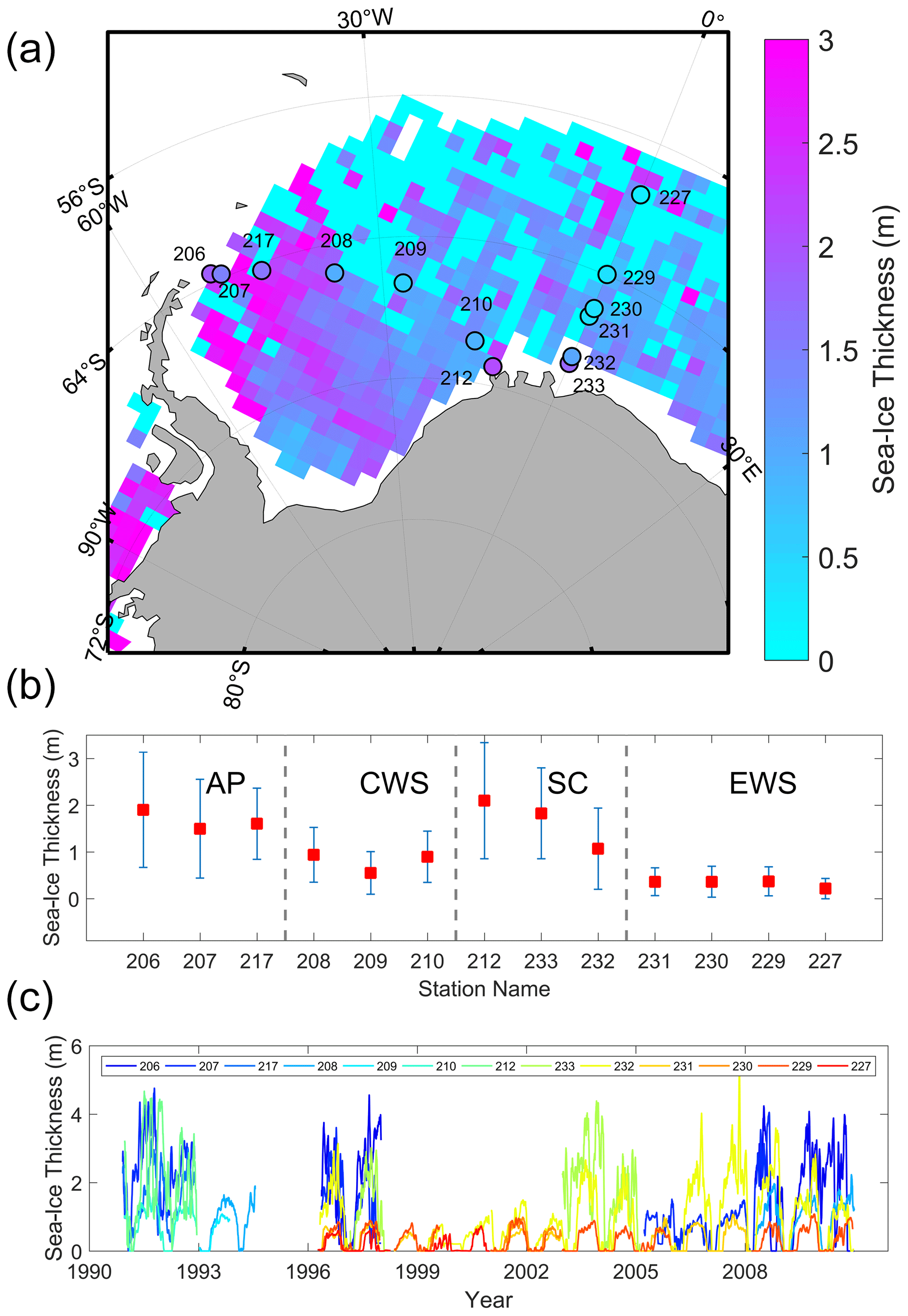
Figure 1 (a) The ICESat-1 sea-ice thickness in the autumn of 2005 in the Weddell Sea and the locations of the moored upward-looking sonars with their mean thicknesses shaded. (b) The mean ULS sea-ice thickness from west to east in the Weddell Sea. The error bars represent the SD of daily ice thickness for individual stations. Dotted gray lines divide the 13 stations into four parts: the Antarctic Peninsula (AP), the central Weddell Sea (CWS), the southern coast (SC) and the eastern Weddell Sea (EWS). (c) The time series of daily sea-ice thickness of all 13 stations based on a 15 d moving average.

In this section, we use sea-ice thickness derived from ULS to evaluate the above-mentioned four reanalyses, as well as other reference observations. All ULS data are recorded once a second and are averaged into a monthly ice draft estimate. Because thick deformed sea ice is found in the southern and western Weddell Sea (Behrendt et al., 2013; Kurtz and Markus, 2012), the 13 ULS stations are divided into four sub-regions (Fig. 1b): the Antarctic Peninsula (AP; including Stations 206, 207 and 217), the central Weddell Sea (CWS; including Stations 208, 209 and 210), the southern coast (SC; including Stations 212, 232 and 233) and the eastern Weddell Sea (EWS; including Stations 227, 229, 230 and 231). The classification criterion is based on the locations of ULS stations (Fig. 1a) and long-term averaged ULS sea-ice thickness, as well as their standard deviation (SD; Fig. 1b). Under this classification, the AP is dominated by deformed thick sea ice and the EWS by newly formed ice. The CWS has both first-year ice and deformed sea ice, and the southern coast has both first-year ice and landfast sea ice (Harms et al., 2001; Behrendt et al., 2013). The aggregate temporal span of ULS observations in AP, CWS, SC and EWS is 148, 73, 185 and 272 months, respectively.

Table 1 Introduction of the four reanalyses data systems used in this study.

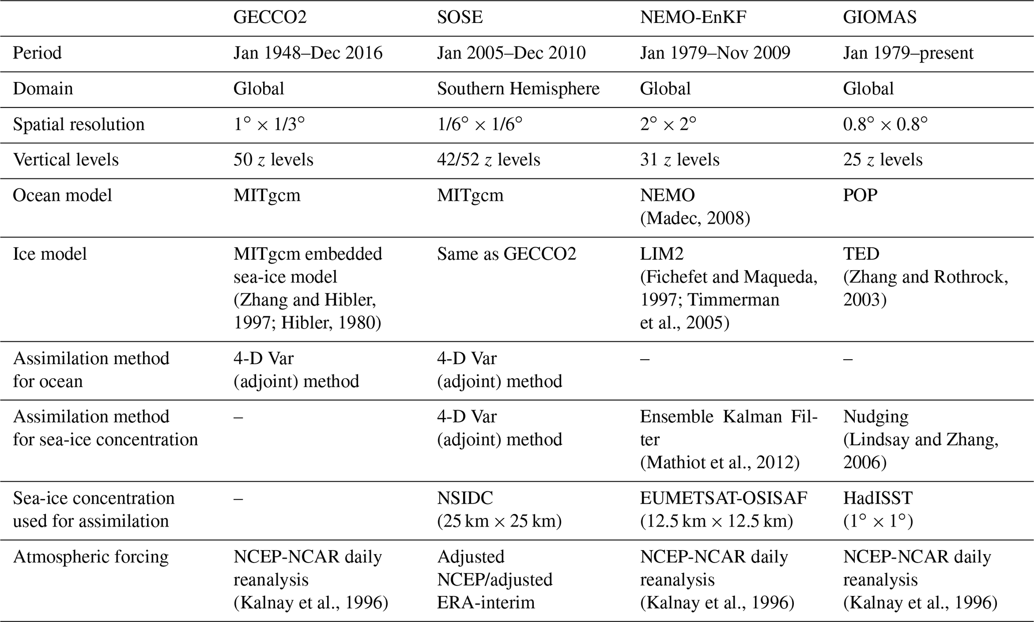
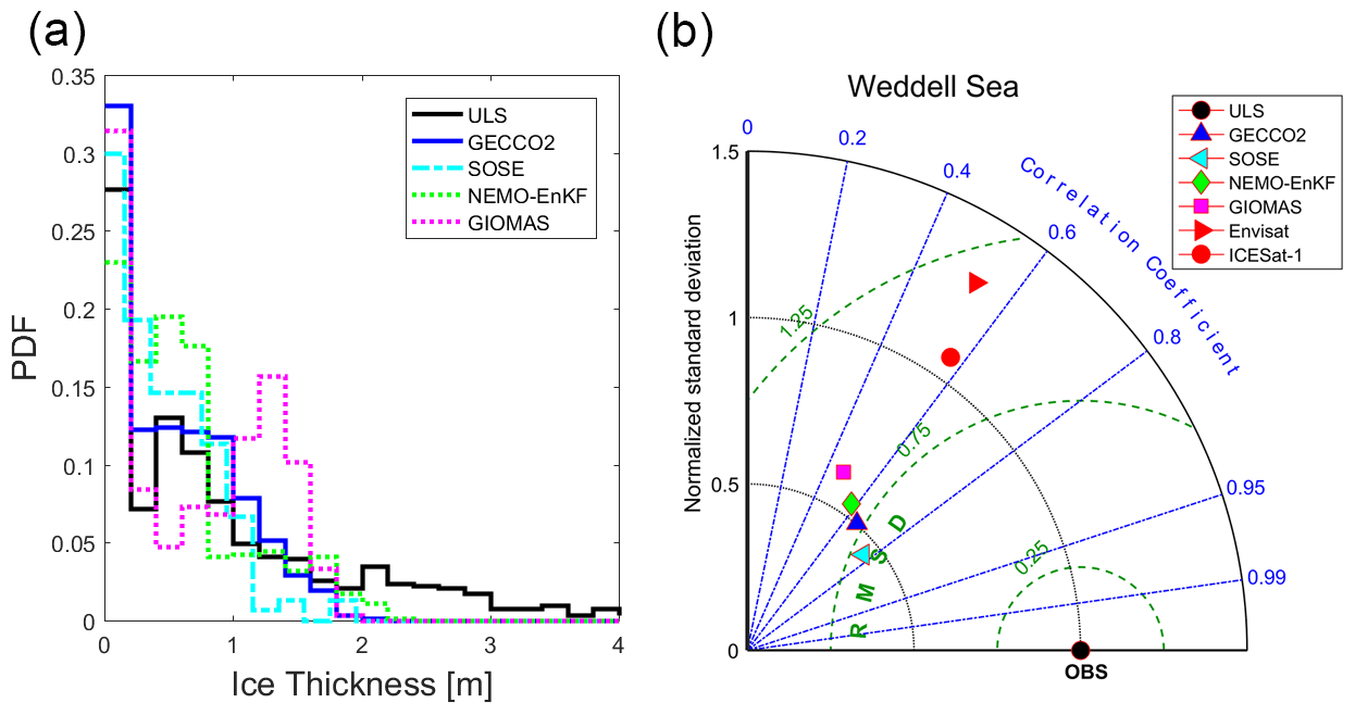
Figure 2 (a) Probability density distributions (PDFs) of monthly sea-ice thickness from ULS and the four reanalyses at the 13 ULS locations of the Weddell Sea. (b) Normalized Taylor diagram for monthly sea-ice thickness of the four reanalyses, as well as Envisat and ICESat-1, with respect to the sea-ice thickness from upward-looking sonar from 1990 to 2008 in the Weddell Sea. The dashed green lines indicate the normalized root mean square error (RMSE).

Then we compare the ice thickness distribution from the reanalyses with ULS observations in 13 positions in the Weddell Sea (Fig. 2a). As presented in Table 1, SOSE has a shorter period than the other three reanalyses. To include the most available data records in the intercomparison, the periods of GECCO2, NEMO-EnKF and GIOMAS are from 1990 to 2008, while the period of SOSE is from 2005 to 2008. The results indicate that for each data set, the most probable sea-ice thickness is less than 0.2 m. The NEMO-EnKF and ULS have local maxima in the distribution of 0.4–0.6 m. GIOMAS has local maxima of 1.2–1.4 m. Meanwhile, the probability density function (PDF) of GECCO2 and SOSE decreases with increasing sea-ice thickness. None of the reanalyses have sea ice thicker than 2.2 m, though thicknesses of this magnitude are observed by ULS (Fig. 2a).

The Taylor diagram (Fig. 2b) indicates that the correlation coefficients (CCs) of all six data sets are larger than 0.4, and SOSE has the highest CC of 0.77. The maximum and minimum root mean square errors (RMSEs) are 1.15 m for Envisat and 0.71 m for SOSE. The normalized SDs (NSDs) of sea-ice thickness from the four reanalysis data sets, divided by the SD of the references, are lower than 0.62, while the NSDs of Envisat and ICESat-1 are larger than 1.0. Compared with the four reanalyses, ICESat-1 has a higher SD that is close to 1.0, which means ICESat-1 could reproduce the variation in sea ice better than the four reanalyses. It is noted that the relatively short ICESat-1 record (13 months) limits the reliability of this assessment.

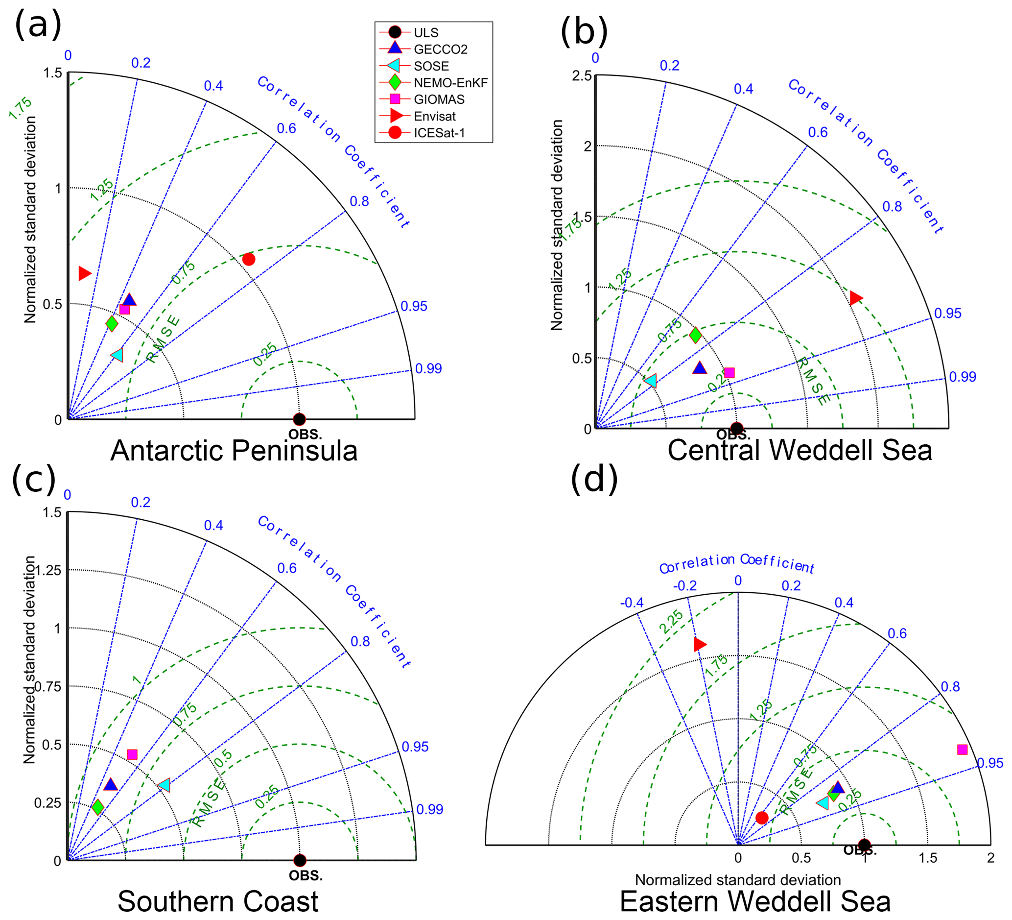
Figure 3 Same as Fig. 1b but for the four sub-regions: (a) Antarctic Peninsula, (b) central Weddell Sea, (c) southern coast and (d) eastern Weddell Sea.

In AP (Fig. 3a), GECCO2, NEMO-EnKF and GIOMAS have CCs around 0.4, and SOSE has the highest CC of 0.62. All RMSEs for the four reanalyses are larger than 0.7 m. The NSDs of the four reanalyses and Envisat are lower than that of the ULSs. ICESat-1 has the largest CC of 0.74 and an NSD of nearly 1.0. In the CWS (Fig. 3b), the CCs of the six data sets are all higher than 0.7. The NSD of GECCO2, SOSE, NEMO-EnKF and GIOMAS is 0.85, 0.52, 0.97 and 1.03, respectively. That means that GECCO2, NEMO-EnKF and GIOMAS could reproduce well the variation in the sea-ice thickness in the CWS. In addition, Envisat overestimates the interannual variability of sea-ice thickness significantly in this region as its NSD is larger than 2.0. On the southern coast (Fig. 3c), the CC of GECCO2, SOSE, NEMO-EnKF and GIOMAS is 0.50, 0.79, 0.50 and 0.52, respectively. The normalized NSD of GECCO2, SOSE, NEMO-EnKF and GIOMAS is 0.37, 0.53, 0.26 and 0.54, respectively, indicating that all reanalyses underestimate the sea-ice thickness variability, especially for NEMO-EnKF. SOSE performs best among the four reanalyses with a high CC of 0.79 and a low RMSE of 0.66 m. In the EWS (Fig. 3d), the CC of GECCO2, SOSE, NEMO-EnKF and GIOMAS is 0.87, 0.90, 0.88 and 0.92, respectively. Their normalized NSD is 0.91, 0.76, 0.86 and 1.93, implying that GECCO2, SOSE and NEMO-EnKF reproduce well the seasonal thickness variation in first-year ice. ICESat-1 has a lower CC of 0.66 and NSD of 0.29, partly resulting from the large uncertainty of ICESat-1 in measuring the first-year ice thickness in this region, particularly in the summertime. Envisat has the lowest CC (−0.19) and highest RMSE (2.06 m) among all data sets, and its NSD is comparable with GIOMAS.

SOSE has larger CCs than the other three reanalyses in the regions close to the coast (AP and SC). Even though SOSE uses the same MITgcm ice–ocean model as GECCO2, its higher spatial resolution of 1∕6^∘ resolves more small-scale dynamical processes in these regions. But in the regions with large amounts of newly formed ice (the CWS and the EWS), SOSE tends to underestimate sea-ice thickness with lower NSDs than the other reanalyses. GECCO2 and NEMO-EnKF have similar statistics in the four sub-regions. They perform best in the regions dominated by newly-formed ice (SC). GIOMAS has a moderate performance in the regions close to the coast and performs best in the CWS, with the highest CC of 0.92 and lowest RMSE of 0.40 m. GIOMAS shows excessive variability in the CWS with an NSD of 1.93.

3.2 Comparisons with ice thickness from the ASPeCt

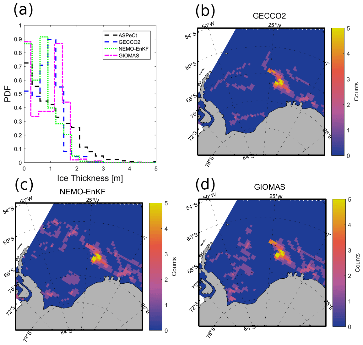
Figure 4 (a) Histograms of sea-ice thickness from ASPeCt and three reanalyses. Locations of model sea-ice thickness are shown in (b) GECCO2 for a range of 0.8 to 1.4 m, (c) NEMO-EnKF for a range of 1.1 to 1.7 m and (d) GIOMAS for a range of 1.1 to 1.7 m.

The monthly sea-ice thickness distribution histograms (Fig. 4a) show that the three reanalyses (GECCO2, NEMO-EnKF, GIOMAS) have distributions suggesting an overestimation of the abundance of thin ice and underestimation of the abundance of thick ice with respect to ASPeCt. We exclude SOSE in the evaluation due to its relatively short period because the ASPeCt observations used here are from 1981 to 2005, though there are extensive ASPeCt observations from 2005 to 2012, but the sample records are very limited in the Weddell Sea. While there are a few instances of sea-ice thicknesses greater than 1.8 m in GECCO2, NEMO-EnKF and GIOMAS, ASPeCt has recorded ice thicker than 3.0 m. Given that the ASPeCt observations from an area with a six nautical mile radius (∼ 11.1 km) are compared with models with ∼ 60 km spatial resolution, this is unsurprising. The ship observations show the pack ice to be a highly varied and complicated mixture of different ice types. The concentration, thickness and topography may vary significantly over a short spatial distance. Compared with ASPeCt, GECCO2 has more sea ice with thicknesses ranging from 0.5 to 1.25 m, and GIOMAS has more sea ice with thicknesses ranging from 1.3 to 1.8 m. NEMO-EnKF mainly overestimates sea-ice thickness within the bins from 0 to 1.0 m. In addition, the sea-ice thicknesses of GECCO2, NEMO-EnKF and GIOMAS seem to be concentrated within the range of 0.8 to 1.4 m, 0.5 to 0.8 m and 1.1 to 1.7 m, respectively (Fig. 4a). These thicknesses are mainly found over the first-year sea-ice area of the eastern Weddell Sea and ice edge (Fig. 4b–d). In these regions, reanalyses tend to overestimate sea-ice thickness in contrast to ASPeCt, which is consistent with the results reported in Timmermann et al. (2005). The small-scale spatial and temporal variation in ice thickness, which is represented in the ASPeCt observations, is not captured by the reanalyses.

Table 2 ICESat-1 measurement periods in this study. Abbreviations given in parentheses in each cell are used throughout the paper to denote the respective period. Spring-ON refers to October and November, Autumn-FM refers to February and March, and Winter-MJ refers to May and June.

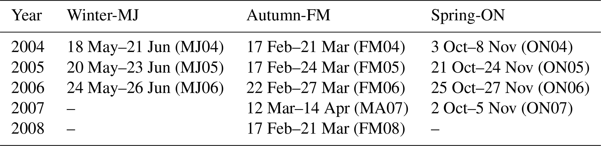
Table 3 The mean ice thickness bias, root mean square error estimate and correlation between ICESat-1 and the four sea-ice thickness reanalyses.

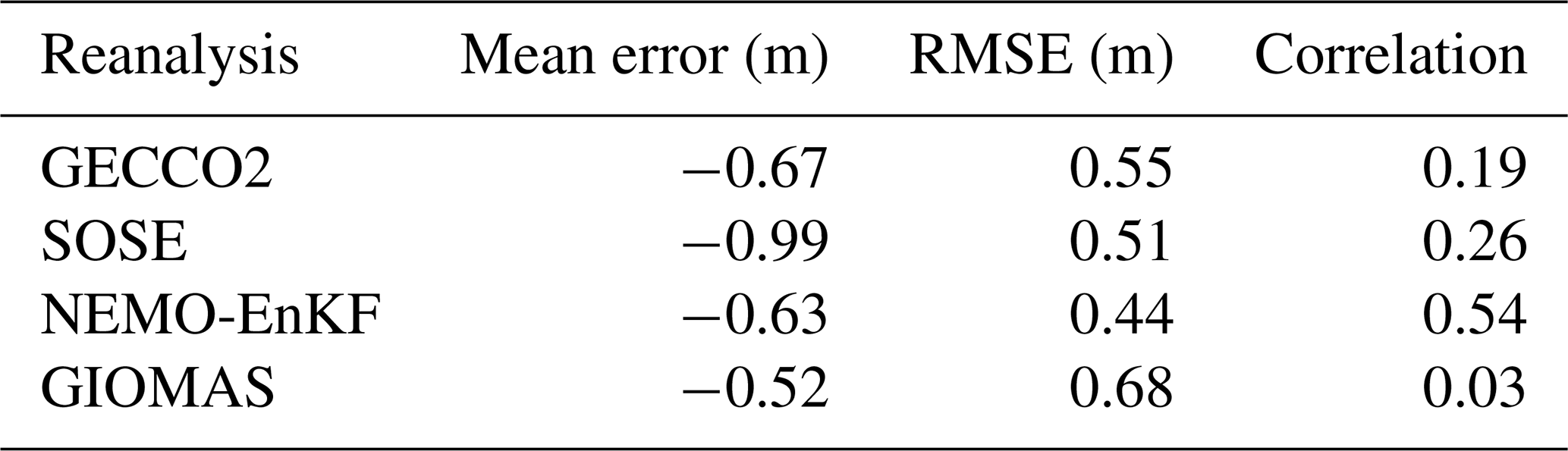
Figure 5 The variation in monthly ice thickness distribution from GECCO2 (blue), SOSE (cyan), NEMO-EnKF (green), GIOMAS (pink) and ICESat-1 (red) in Autumn-FM (a), Winter-MJ (b) and Spring-ON (c). The colored dots represent the modal ice thickness.

3.3 Comparison with sea-ice thickness from ICESat-1

In this section, we compare sea-ice thickness from the four reanalyses (GECCO2, SOSE, NEMO-EnKF and GIOMAS) with that from ICESat-1 for the period from 2005 to 2008. Considering the fact that ICESat-1 does not always provide data for full months, we perform a time-weighted calculation for all four reanalyses in the comparison. For example, the temporal span of February to March 2004 (FM04) is from 17 January to 21 March, which includes 13 d in February and 21 d in March; therefore, all sea-ice thickness (SIT) reanalyses are averaged by $(\mathrm{13}/\mathrm{34})\cdot {\text{SIT}}_{\text{Feb}}+(\mathrm{21}/\mathrm{34})\cdot {\text{SIT}}_{\text{Mar}}$. Based on the statistics of aggregate sea-ice thickness, all four reanalyses underestimate ice thickness close to 1 m (Table 3). The RMSEs of the four reanalyses exceed 0.6 m, and the maximum and minimum RMSEs are 0.8 m (GIOMAS) and 0.6 m (SOSE), respectively. The correlations between the four reanalyses and ICESat-1 are low, and the maximum correlation coefficient is only 0.31 (NEMO-EnKF). It should be noted that the ICESat-1 records are very limited; they are only from October, November, February, March, May and June (see Table 2 for more information). Following Kern and Spreen (2015) and Kern et al. (2016), when comparing with ICESat-1, we use October and November to represent spring (hereafter Spring-ON), February and March to represent autumn (hereafter Autumn-FM), and May and June to represent winter (hereafter Winter-MJ). Based on the interannual variation in ice thickness distribution (ITD) from Autumn-FM to Spring-ON (Fig. 5), we find that ICESat-1 thickness is much thicker than that of the reanalyses except GIOMAS in Spring-ON. The ITD of ICESat-1 shows peaks mainly around 1.2 m (ice thickness < 0.5 m are truncated), while the four reanalyses have peaks in the low sea-ice thickness bins (< 1.0 m) and very little ice thicker than 2.0 m. The modal sea-ice thickness of ICESat-1 has a weak interannual variation in different seasons (red dots in Fig. 5), but the modal sea-ice thicknesses of NEMO-EnKF and GIOMAS have significant interannual variation in Autumn-FM. In addition, the modal and mean ice thicknesses of ICESat-1 have significant seasonal variation (e.g., modal thickness decreases from 1.7 to 0.9 m from austral Autumn-FM to Winter-MJ due to the new ice formation and increases to 1.3 m from Winter-MJ to Spring-ON due to the thermodynamic and dynamic processes). In most cases, modal ice thickness of the reanalyses is lower than that of ICESat-1. For example, in 2008 Autumn-FM, the four reanalyses have modal ice thickness lower than 0.3 m, indicating the newly formed sea ice. However, ICESat-1's modal ice thickness is around 1.5 m. SOSE and NEMO-EnKF have a similar variation in modal ice thickness from Autumn-FM to Spring-ON to ICESat-1 in 2005 and 2006. GIOMAS has a similar seasonal variation in 2005. GECCO2 fails to reproduce the decrease in modal ice thickness from Autumn-FM to Winter-MJ. This is because GECCO2 loses the most thick ice in summer and thus has lower modal ice thickness than the other data sets.

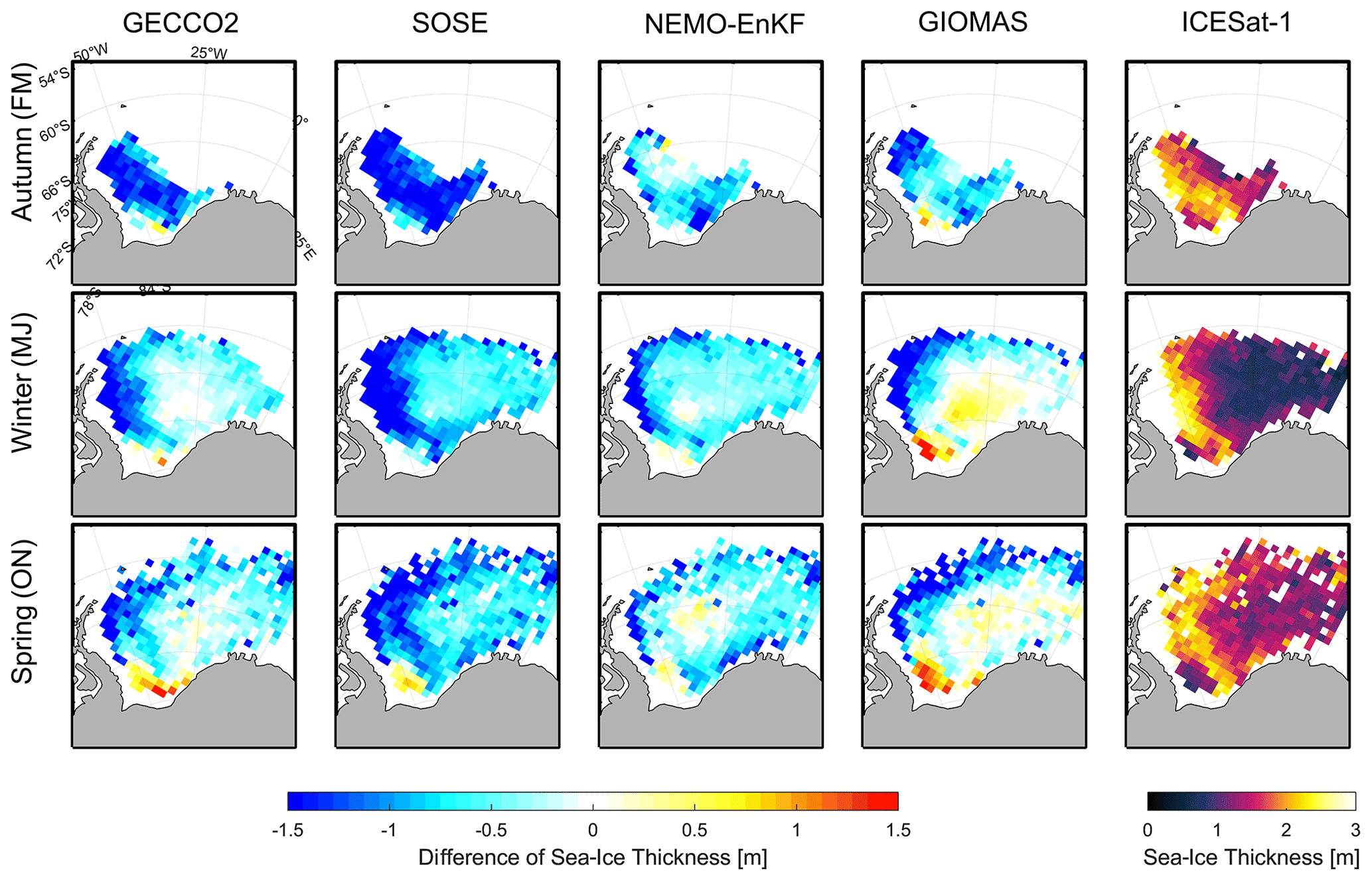
Figure 6 The differences of sea-ice thickness between GECCO2 (first column), SOSE (second column), NEMO-EnKF (third column), GIOMAS (fourth column) and ICESat-1 in Autumn-FM (first row), Winter-MJ (second row) and Spring-ON (third row).The contours in last column represent the autumn sea-ice thickness of ICESat-1.

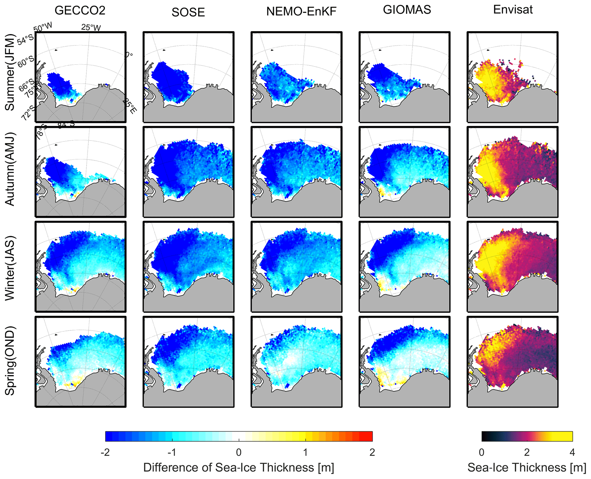
Figure 7 Same as Fig. 6 but with respect to Envisat (last column) for the 4 year period 2005–2008.

In addition to the aggregate sea-ice thickness statistics, the spatial difference of the thicknesses between the four analyses and ICESat-1 is also investigated. The ICESat-1 data show ice thicker than 2.5 m, mainly located in the western Weddell sea and with a location shifting from the southwestern Weddell Sea in Autumn-FM to the northwestern Weddell Sea in Spring-ON (Fig. 6). In Autumn-FM, all reanalyses underestimate ice thickness. For GECCO2 and SOSE, negative biases up to 1.5 m almost cover the entire Weddell Sea, and the negative biases of NEMO-EnKF and GIOMAS mainly occur in the area near the coast. Considering that the ICESat-1 thickness may be biased low (Kern et al., 2016), this suggests that these reanalyses may not represent coastal processes well. The spatially averaged differences between models and ICESat-1 are −1.30 m (GECCO2), −0.63 m (NEMO-EnKF) and −0.75 m (GIOMAS), respectively. In Winter-MJ, all reanalyses still underestimate sea-ice thickness along the Antarctic Peninsula (AP) and in the western Weddell Sea, and GIOMAS overestimates thickness in the CWS and near the Ronne Ice Shelf of the southern Weddell Sea, where new sea ice is found. All four reanalyses underestimate sea-ice thickness by up to 1.5 m in the north edge of sea-ice cover. In Spring-ON, the area of thickness underestimation of all four analyses shrinks to the western Weddell Sea along the AP and the northern edge of ice cover, while a slight overestimation is also found in the central and eastern Weddell Sea. In addition, GIOMAS overestimates ice thickness near the Ronne Ice Shelf in the southern Weddell Sea, which is thought to be an important source of new sea ice (Drucker et al., 2011). The overestimation is likely due partially to GIOMAS's explicit simulation of sea-ice ridging processes, which tends to create thick ridges. It may also be due to the generally low ICESat-1 thickness values when compared to ULS and Envisat data (see Fig. 3d above).

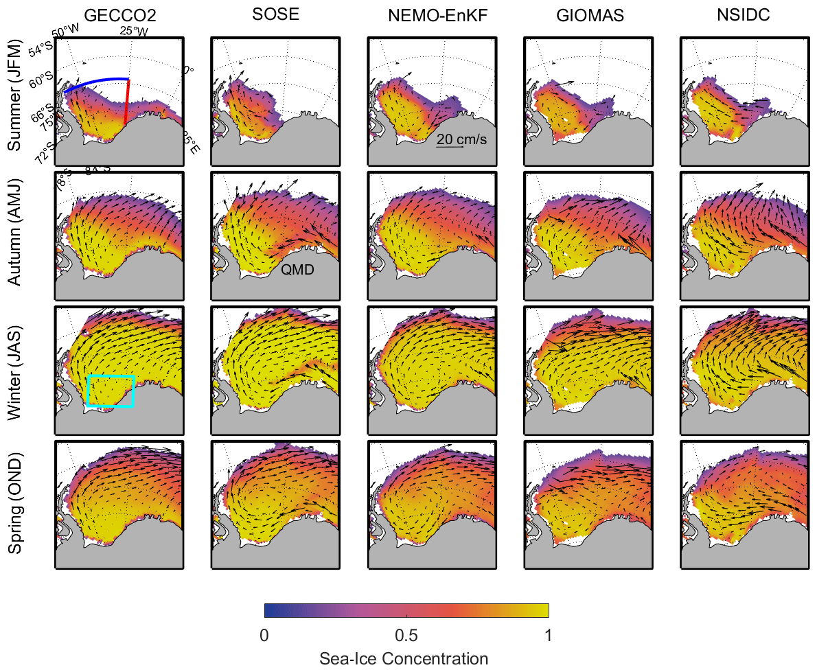
Figure 8 Seasonal mean sea-ice concentration (summer to spring) for the 4 year period 2005–2008. The overlapped vectors represent sea-ice velocity from respective data sets.

3.4 Comparison with seasonal evolution of sea-ice thickness from Envisat

The comparison with ICESat-1 thickness in Sect. 3.3 is limited by the temporal coverage of ICESat-1; in particular, the seasonal evolution cannot be fully quantified. Although the Envisat sea-ice thickness has larger biases than ICESat-1 thickness (Schwegmann et al., 2016; Wang et al., 2020), it is still useful in assessing the seasonal evolution of the sea-ice thickness due to it covering all seasons. Furthermore, its spatial distribution has a good spatial correlation with ICESat-1 (figure not shown here).

In this section, based on the Envisat sea-ice thickness data, we focus on the comparison of seasonal variation in the spatial distribution of sea-ice thickness averaged from 2005 to 2008. Following the seasonal classification in Holland and Kwok (2012), the summer, autumn, winter and spring hereinafter refer to January to March, April to June, July to September and October to December, respectively. The spatial distribution of sea-ice thickness of NEMO-EnKF shows the most similarity with Envisat over the year (Fig. 7). GECCO2 and SOSE have similar sea-ice thickness distributions all year round, while GECCO2 is much thicker. The thickest ice of GECCO2 and SOSE is mainly located in the southern Weddell Sea and the southwestern Weddell Sea, respectively. NEMO-EnKF reproduces the thick sea ice (> 1.5 m) over the region in the northwestern Weddell Sea from winter to spring. Compared with other models, GIOMAS has the largest amount of thick ice (> 2.0 m), and it is mostly located in the western and southern Weddell Sea and occurs in all seasons. In addition, different from other data sets, GIOMAS has a large area of sea ice thicker than 1.5 m between −25^∘ W and 0^∘ E over the eastern Weddell Sea from autumn to spring.

The sea-ice concentration is also analyzed as it is closely tied to sea-ice thickness via dynamics and thermodynamics. Benefiting from data assimilation approaches, all models have a similar spatial distribution of sea-ice concentration with respect to satellite observations (Fig. 8). GECCO2, which has not assimilated sea-ice concentration, has a high concentration in the southern Weddell Sea, while the other three models have high concentrations found mostly in the southwestern Weddell Sea. It is worth noting that the SOSE sea-ice concentration shows a “river” pattern with a relatively low sea-ice concentration around the prime meridian in autumn and winter. This phenomenon can be attributed to the open-ocean polynya in 2005, and it has also been reported by Abernathey et al. (2016).

Figure 9 Same as Fig. 9 but for the divergence of sea-ice motion.

Driven by wind and underlying ocean currents, sea-ice motion shapes the dynamic thickening of sea ice. We investigate the sea-ice motion effects on the spatial distribution of sea-ice thickness. Because Envisat does not measure ice motion, the satellite ice motion data product from the National Snow and Ice Data Center is used instead (Tschudi et al., 2019). In addition, we also calculate the divergence of ice motion to investigate the influence of ice motion on the variation in sea-ice thickness. Figure 8 shows that a clockwise ice motion is the leading pattern in the Weddell Sea, known as the Weddell Gyre, especially in wintertime. GECCO2 has weak ice motion and weak convergence in the southern Weddell Sea (the cyan rectangle in Fig. 9), while the other three reanalyses show an apparent westward ice motion. That gives rise to less ice accumulation along the AP in GECCO2. In addition, the westward movement of the SOSE, NEMO-EnKF and NSIDC ice velocity fields with ice convergence in the southwestern Weddell Sea are in favor of the dynamic thickening. Compared to NEMO-EnKF and GIOMAS in summer through autumn, SOSE has a stronger sea-ice circulation advecting more ice toward the northwestern Weddell Sea and the coast of the AP. SOSE has rapid ice motion for all seasons, especially near the Antarctic Peninsula in the western Weddell Sea and the coast near Queen Maud Land (QMD) in the southern Weddell Sea. The high ice speed of SOSE in this region may result from its relatively thin sea ice. Based on the satellite data, the convergence is mainly in the middle and eastern Weddell Sea. The divergence is mainly in the southern and western Weddell Sea, which are the regions of new sea-ice formation and sea-ice deformation, respectively (Fig. 8). GECCO2 mainly has convergence in all seasons. The strong divergence and convergence of SOSE alternatively occur in the southeastern Weddell Sea and the northern edge of the sea-ice cover. The sea-ice motion convergence of NEMO-EnKF is relatively weak but widespread and is generally consistent with satellite inferences. GIOMAS shows an abnormal divergence in the eastern Weddell Sea in autumn, which may result from its thick ice in this region, diagnosed in Sect. 3.3.

Table 4 Mean sea-ice volume flux biases, root mean square error and correlation through the 25^∘ W and 65^∘ S sections between the four reanalyses and satellite observations. (Unit: 10³ km² month⁻¹; positive/negative sign means the outflow and inflow into the regions outlined by red and blue lines in Figs. 8 and 9.)

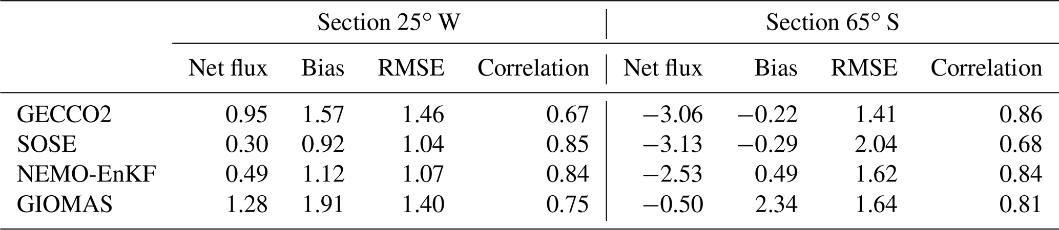
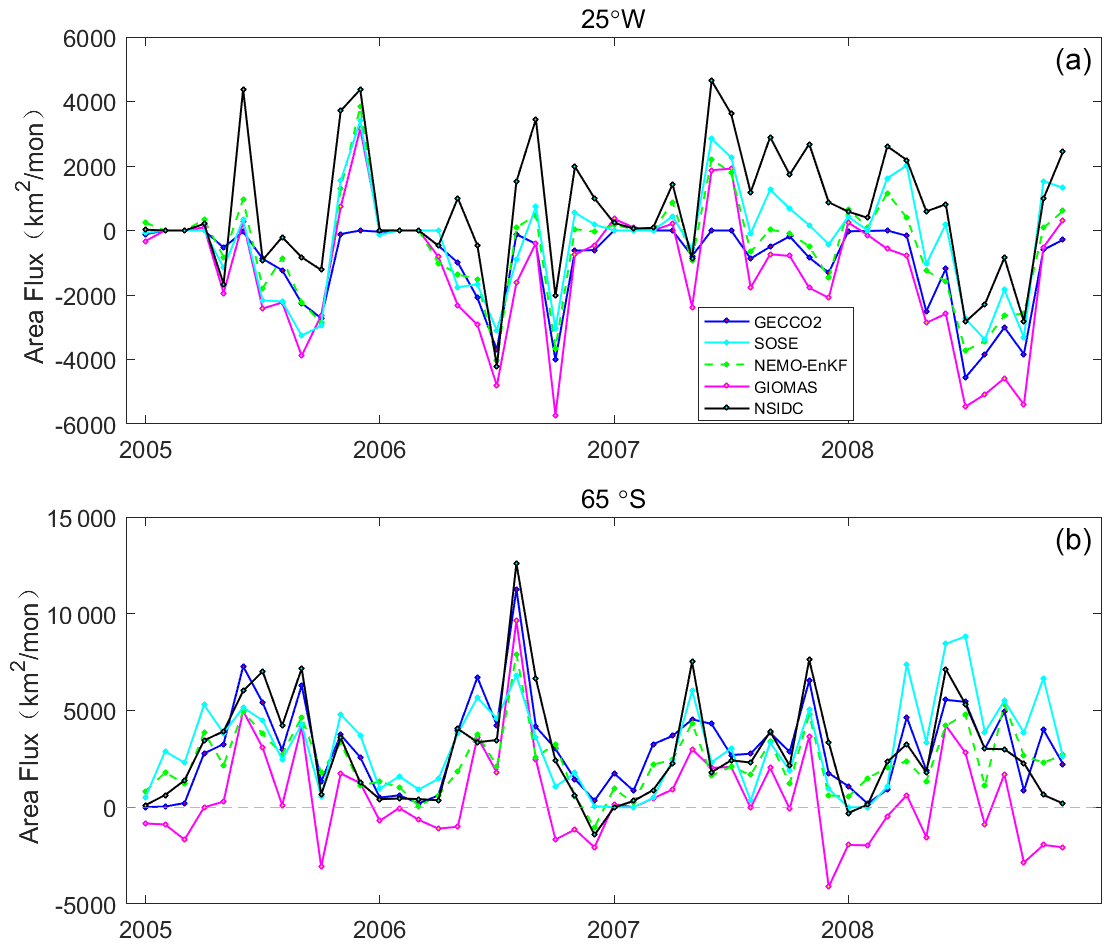
Figure 10 (a) Monthly sea-ice area flux westward into the southwestern Weddell Sea across the 25^∘ W section and (b) area flux northward out of the southwestern Weddell Sea across the 65^∘ S section from 2005 to 2008.

In order to quantitatively estimate the influence of sea-ice advection on thickness in the southwestern Weddell Sea, we calculate sea-ice flux across two sections. The zonal section (from 70 to 25^∘ W, 65^∘ S) captures outflow from the western Weddell Sea (Harms et al., 2001). Flux across the meridional section (65 to 72^∘ S, 25^∘ W) is also diagnosed to form a closure (Fig. 8, blue and red line). Here, we use sea-ice area flux instead of the volume flux to exclude the thickness influence. All models underestimate the sea-ice area flux across 25^∘ W, especially for GECCO2 and GIOMAS (Fig. 10a). The ice area flux in GIOMAS is approximately half of that in the NSIDC product (Table 4). In the 65^∘ S section, GIOMAS has a smaller northward ice area flux which favors thick ice staying in the southwestern Weddell Sea. With respect to the NSIDC product, GECCO2 and SOSE have relatively small ice inflows in the 25^∘ W section (0.95 × 10³ and 0.30 × 10³ km² month⁻¹) and relatively high outflow in the 65^∘ S section (3.06 × 10³ and 3.13 × 10³ km² month⁻¹), which favors thin ice in the southwestern Weddell Sea. SOSE and NEMO-EnKF have similar ice fluxes in the 25^∘ W section, but NEMO-EnKF has better ice thickness distribution than SOSE, according to Fig. 7. NEMO-EnKF has a smaller ice flux in the 65^∘ S section and a better correlation with NSIDC. We find that accurate northward ice motion in the western Weddell Sea is related to thick ice accumulation in the southwestern Weddell Sea and that sea-ice thickness distribution is consistent with observations.

4 Discussion and summary

In this paper, we evaluate sea-ice thickness in the Weddell Sea from the four reanalyses against observations from satellite altimeters, mooring and visual observations. It should be noted that although this evaluation is based on most of the available observations in the Weddell Sea, there are still uncertainties and limitations in this evaluation. For example, due to the temporal coverage of the reanalyses and reference data, the large-scale evaluation against ICESat-1 and Envisat is limited to 2005 to 2008, and it mainly focuses on the seasonal evolution and spatial distribution of ice thickness. The evaluation against ASPeCt is from 1981 to 2005. Furthermore, Schwegmann et al. (2016) have shown that Envisat sea-ice thickness underestimates thick ice and overestimates thin ice compared to CryoSat-2. In addition, the Envisat sea-ice thickness has different interannual variability compared to the in situ ULS observations. Nevertheless, the Envisat thickness has still been used to investigate the seasonal evolution of sea ice in this study. These limitations should be further addressed when more ice thickness observations are available in the future.

Table 5 Statistics of the four reanalyses with respect to ULS and ICESat-1.

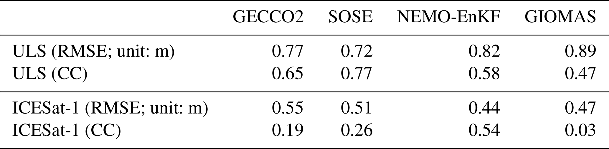
To further quantitatively measure the performance of all four, we use the RMSE and correlation coefficient (CC) with respect to ULS and altimeter measurements as criteria. It is noted that the CC with ULS means the temporal correlation between the four reanalyses and ULS, while the CC with ICESat-1 means the spatial correlation because they are calculated by yearly mean SIT fields. Our results (Table 5) show that the SOSE has the highest CC of 0.77 and lowest RMSE of 0.72 m when compared with ULS ice thickness. All RMSEs are less than 0.9 m, and all CCs are more than 0.4. Compared with ICESat-1, NEMO-EnKF has the highest CC of 0.54 and lowest RMSE of 0.44 m. CCs of the other three reanalyses are less than 0.3, and GIOMAS has almost no spatial relation with ICESat-1.

We conclude that current sea-ice thickness reanalyses in the Weddell Sea have a varying degree of accuracy. Compared with ASPeCt, GECCO2, NEMO-EnKF and GIOMAS have deficiencies in reproducing the small spatiotemporal variation in thickness in regions dominated by first-year ice. Compared with ICESat-1 and ULS sea-ice thicknesses, all four reanalyses underestimate ice thickness in the western and northwestern Weddell Sea with highly deformed sea ice (mean ice thickness > 1.5 m) from Autumn-FM to Spring-ON. To be particular, GIOMAS and SOSE ice thicknesses perform the best on the central and the southern coasts of the Weddell Sea, respectively, while GECCO2 and NEMO-EnKF could reproduce well new ice evolution in the eastern Weddell Sea. GIOMAS tends to overestimate first-year ice thickness in the eastern Weddell Sea, especially in spring. Besides the explicit simulation of ice ridging, the convergence of GIOMAS sea ice in the CWS may be an important cause of the positive bias in sea ice for this reanalysis. Compared with Envisat, only NEMO-EnKF did well in reproducing the clockwise shift of thick ice from the western Weddell Sea in winter to the northwestern Weddell Sea in spring. Our study also indicates that the northward ice motion in the western Weddell Sea along the Antarctic Peninsula has an important influence on ice thickness distribution in the Weddell Sea.

This study shows that to accurately infer the variability in the Antarctic sea-ice volume (not only the Weddell Sea) in the context of global climate change, there is still room to further improve the Antarctic sea-ice reanalyses, and possible ways include improving the ice–ocean model physics by optimizing model parameters (e.g., Sumata et al., 2019) and assimilating ice–ocean observations (in particular the satellite-derived sea-ice thickness) with a ocean–sea-ice multi-variate data assimilation approach (e.g., Mu et al., 2020).