Contrasting regional variability of buried meltwater extent over 2 years across the Greenland Ice Sheet

The Greenland Ice Sheet (GrIS) rapid mass loss is primarily driven by an increase in meltwater runoff, which highlights the importance of understanding the formation, evolution, and impact of meltwater features on the ice sheet. Buried lakes are meltwater features that contain liquid water and exist under layers of snow, firn, and/or ice. These lakes are invisible in optical imagery, challenging the analysis of their evolution and implication for larger GrIS dynamics and mass change. Here, we present a method that uses a convolutional neural network, a deep learning method, to automatically detect buried lakes across the GrIS. For the years 2018 and 2019 (which represent low- and high-melt years, respectively), we compare total areal extent of both buried and surface lakes across six regions, and we use a regional climate model to explain the spatial and temporal differences. We find that the total buried lake extent after the 2019 melt season is 56 % larger than after the 2018 melt season across the entire ice sheet. Northern Greenland has the largest increase in buried lake extent after the 2019 melt season, which we attribute to late-summer surface melt and high autumn temperatures. We also provide evidence that different processes are responsible for buried lake formation in different regions of the ice sheet. For example, in southwest Greenland, buried lakes often appear on the surface during the previous melt season, indicating that these meltwater features form when surface lakes partially freeze and become insulated as snowfall buries them. Conversely, in southeast Greenland, most buried lakes never appear on the surface, indicating that these features may form due to downward percolation of meltwater and/or subsurface penetration of shortwave radiation. We provide support for these processes via the use of a physics-based snow model. This study provides additional perspective on the potential role of meltwater on GrIS dynamics and mass loss.

1 Introduction

The Greenland Ice Sheet (GrIS), which holds enough ice to raise sea level globally by more than 7 m (Smith et al., 2020), has experienced net mass loss every year since 1998 (Mouginot et al., 2019). Since 1972, the GrIS has contributed a total of 13.7 ± 1.1 mm of sea level rise. Prior to 2005, ice discharge was the primary driver of Greenland mass loss (Enderlin et al., 2014). However, meltwater runoff, which has accelerated recently, is now the dominant factor in Greenland mass loss (Smith et al., 2020; van Den Broeke et al., 2016; Enderlin et al., 2014). Thus, surface melt plays an increasingly important role in the mass balance of the GrIS.

Melting is exacerbated by the positive melt–albedo feedback, whereby melting acts to lower surface albedo, which in return allows for greater absorption of incoming solar radiation, thus further enhancing surface melt (Box et al., 2012; Lüthje et al., 2006; Tedesco et al., 2012). Meltwater often pools in surface lakes in the ablation zone during the summer from May to October (McMillan et al., 2007; Banwell et al., 2012). Water in these lakes then runs off the ice sheet, drains via hydrofracture (Das et al., 2008; Tedesco et al., 2013; Williamson et al., 2018b), or refreezes in the firn (Bell et al., 2018). Firn takes up meltwater and buffers against mass loss (Harper et al., 2012). Water that refreezes in near-surface firn leads to the formation of ice lenses, which increase the density and decrease the porosity of the near-surface firn, thus reducing the capacity of Greenland's firn to hold future meltwater (Machguth et al., 2016). Ice lenses due to refrozen meltwater are rapidly increasing in areal extent across the GrIS, leading to increased runoff (MacFerrin et al., 2019; Culberg et al., 2021).

However, not all meltwater stored within the firn refreezes. In fact, some meltwater remains liquid, buried several metres below the surface (Koenig et al., 2015). These shallow buried lakes (or subsurface lakes) have been discovered later in the summer and at higher elevations on the GrIS than their surface counterparts (Miles et al., 2017; Lampkin et al., 2020). Liquid water exists in buried lakes even throughout the winter (Schröder et al., 2020), and some have been shown to rapidly drain, delivering liquid water to the bedrock during the winter months (Benedek and Willis, 2021).

Because meltwater runoff is the dominant driver of mass loss from the GrIS, developing methods to detect surface water has been the focus of many recent studies (Yuan et al., 2020; Sundal et al., 2009; Williamson et al., 2017; Liang et al., 2012). Many of these methods, however, rely on optical imagery to detect meltwater. Buried lakes, in contrast, are invisible in optical images, challenging the study of their extent, evolution, and interaction with drainage systems using conventional methods. More recently, studies have begun using synthetic aperture radar (SAR) to detect both surface and buried lakes (Miles et al., 2017; Johansson and Brown, 2012; Dunmire et al., 2020; Schröder et al., 2020; Benedek and Willis, 2021). As an active sensor, SAR does not require a light source and thus is useful at night or during the polar winter. The European Space Agency's Sentinel-1 satellite uses C-band radiation, which is particularly useful because it is capable of penetrating clouds, ice, and snow up to several metres (Rignot et al., 2001). Water is a strong absorber of C-band SAR radiation. Because of this, Sentinel-1 microwave backscatter can be used as a diagnostic indicator of both the presence of melt and melt intensity and can even detect liquid meltwater buried beneath several metres of ice and snow (Miles et al., 2017).

Fast, automatic detection of buried water features across large spatial and temporal scales is an important step in better understanding their impact on GrIS mass balance. In this study we develop a convolutional neural network (CNN), a deep learning technique for automatic detection of features from images, to detect buried lakes across the GrIS. CNNs are beneficial for feature detection because of their ability to learn spatial relationships from two-dimensional images, and because they can easily be applied across large spatial and temporal scales. CNNs are becoming an increasingly popular choice for automatic feature detection in polar regions and have been used for detecting features such as glacier calving margins (Mohajerani et al., 2019; Zhang et al., 2019), icebergs (Rezvanbehbahani et al., 2019), sea ice concentration (Wang et al., 2016, 2017; Cooke and Scott, 2019; Song et al., 2019), and surface water (Daneshgar et al., 2019; Yuan et al., 2020). Here, we develop and use a CNN to compare the distribution of buried lakes in Greenland's six subregions (Rignot and Mouginot, 2012) during a relatively cold, low-melt year (2018) and a warmer, high-melt year (2019). We compare both buried lake distribution and surface lake distribution between the 2 years and subsequently use a regional climate model to help explain the spatial and temporal differences. Finally, by investigating optical imagery acquired prior to the date of the SAR imagery used here for buried lake detection, we hypothesize that different processes are responsible for the formation of these features in different regions of the GrIS.

2 Methods

2.1 Buried lake detection

2.1.1 Training/testing dataset preparation

Our study region covers the entire GrIS. To create training and testing datasets, we collected Sentinel-2 (S2) optical imagery and Sentinel-1 (S1) C-band SAR microwave backscatter imagery from all six GrIS subregions (Rignot and Mouginot, 2012). S2 images were collected during the late summer (September) of 2016 and 2017, and S1 images were collected during the winter between January 1 and January 7 following the 2018 and 2019 melt seasons. S1 images were chosen during the winter to minimize firn saturation that can obscure buried lakes in microwave imagery. Google Earth Engine (Gorelick et al., 2017) (GEE) was used to collect all images used in this study. GEE preprocesses S1 images with the following steps: (1) thermal noise removal, (2) radiometric calibration, (3) terrain correction using ASTER DEM, and (4) values converted to decibels via log scaling. S2 images are available as top-of-atmosphere reflectance divided by 10 000. All S1 and S2 images exported from GEE were rescaled to 30×30 m resolution (to increase processing speed) on the same grid using nearest-neighbour resampling and reprojected to an Arctic stereographic grid (EPSG:3995). Images were broken up into 256×256 and 512×512 pixel tiles, all resized to 256×256 pixels using a first-order spline interpolation. For each tile, a false-colour image was created using both the S1 and S2 imagery. The false-colour images are made up of the following bands.

• Band 1 = greyscale (from S2) = 0.299 ⋅ red + 0.5870 ⋅ green + 0.1140 ⋅ blue.

• Band 2 = horizontally transmitted − vertically received (HV) band (from S1) normalized from 0 to 1 with respect to the individual image tile such that the minimum tile pixel is 0 and the maximum tile pixel is 1. The purpose of this band is to emphasize microwave backscatter changes that result from the presence of liquid water.

• Band 3 = HV band (from S1) normalized between −30 and 0. This band functions to mute backscatter changes that are small with respect to the surrounding area and thus not likely due to the presence of buried liquid water.

Image tiles were manually classified into seven different categories (1) uniform ice and snow (Fig. 1a, 1277 tiles total), (2) textured ice and snow (Fig. 1b, 1362 tiles total), (3) surface lake remnants (Fig. 1c, 1322 tiles total), (4) open ocean and sea water (Fig. 1d, 99 tiles total), (5) buried lakes (Fig. 1e, 1399 tiles total), (6) land (Fig. 1f, 542 tiles total), and (7) mountains surrounded by snow (Fig. 1g, 227 tiles total). A total of 70 % of the image tiles for each class were used for model training, 15 % for model validation during the training process, and 15 % for a final model test. The training dataset was augmented such that at each iteration of model training, image tiles were randomly flipped horizontally and/or rotated by a random increment of 30^∘.

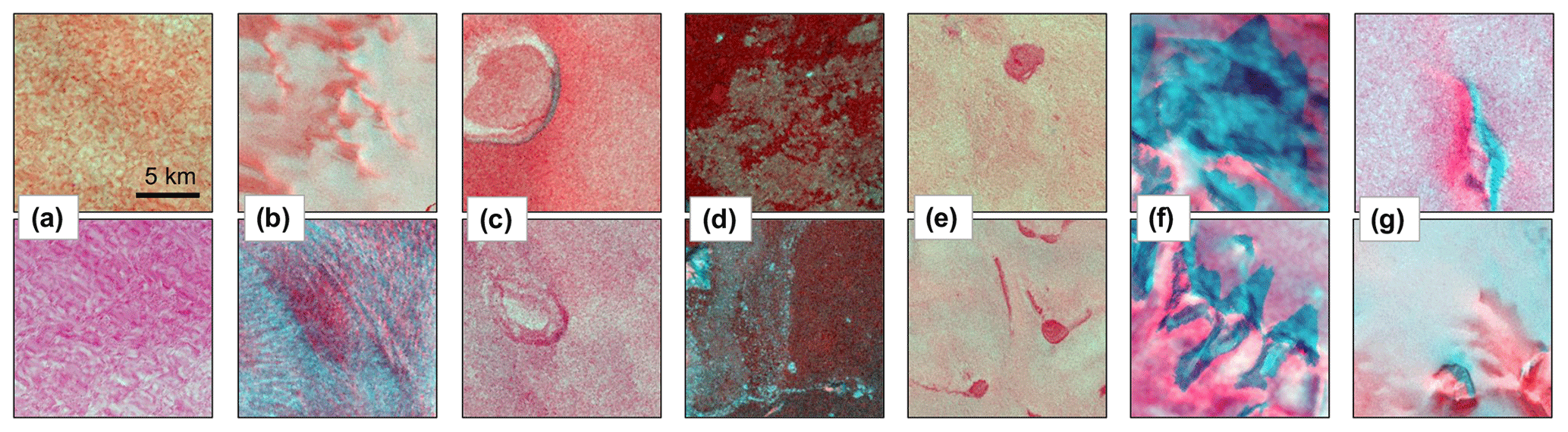
Figure 1 Two example false-colour image tiles for each class used for CNN training. (a) Class 1: uniform ice and snow. (b) Class 2: textured ice and snow including bare ice regions (above) and crevassed regions (below). (c) Class 3: surface lake remnants. (d) Class 4: open ocean and sea water. (e) Class 5: buried lakes. (f) Class 6: land. (g) Class 7: mountains surrounded by snow.

2.1.2 Model training

A CNN was the method of choice for detecting subsurface lakes across Greenland. Unsupervised learning has been shown to be unsuitable for similar analysis on Antarctica (Moussavi et al., 2020), and CNNs have proven superior over other supervised classification algorithms at detecting surface water on Greenland (Yuan et al., 2020). CNNs are being increasingly used for land and surface classification problems (Maggiori et al., 2017). Here, we use the pre-trained AlexNet architecture (Krizhevsky et al., 2012) because it outperformed other model architectures on our validation dataset (Appendix Table A1). To optimize the model for our specific goal of detecting buried lakes, the fully connected layer was rebuilt using one which we designed. This layer used the rectified linear unit (ReLU) activation function (Hara et al., 2015) to solve the vanishing gradient problem and implemented a dropout layer to prevent the model from overfitting (Srivastava et al., 2014). To optimize model parameters, we used the negative likelihood log loss function and Adam optimizer (Kingma and Ba, 2015). The learning rate began as 0.005, decreasing by a factor of 0.1 every seven epochs using a scheduler. Our model was trained for 20 epochs with a batch size of 32 false-colour training image tiles. Finally, our model was further optimized by feeding incorrectly classified tiles back into the training dataset.

2.1.3 Model evaluation and testing

Two different methods were used to evaluate model performance: F1 score and receiver operating characteristic (ROC) curves. F1 score (Eq. 1) is the harmonic mean of precision and recall. Precision (Eq. 2) is essentially a measure of how many positive classifications are actually buried lakes, while recall (Eq. 3) is a measure of how many buried lakes are correctly classified.

$$\begin{array}{}\text{(1)}& {\displaystyle }\mathrm{F}\mathrm{1}={\displaystyle \frac{\mathrm{precision}\cdot \mathrm{recall}}{\mathrm{precision}+\mathrm{recall}}}\text{(2)}& {\displaystyle }\mathrm{Precision}={\displaystyle \frac{\mathrm{TP}}{\mathrm{TP}+\mathrm{FP}}}\text{(3)}& {\displaystyle }\mathrm{Recall}={\displaystyle \frac{\mathrm{TP}}{\mathrm{TP}+\mathrm{FN}}}\end{array}$$

TP is true positive, FP is false positive, and FN is false negative.

Our second model performance metric is a ROC curve. This metric compares true and false positive rates at different classification thresholds. For example, with a threshold of 0, any image tile that the model says has > 0 % chance of being a buried lake is classified as such. Thus, at a threshold of 0, all image tiles will be classified as buried lakes, and there will be high true and false positive rates. Similarly, for a threshold of 1, no image tiles will be classified as buried lakes, and there will be low true and false positive rates. The area under the ROC curve (AUC) is used as an evaluation of model performance, with a larger AUC corresponding to better models.

Appendix Table A1 compares F1 score and AUC for all model architectures we trained to detect buried lakes. Our initial iteration of AlexNet had a relatively high recall and low precision. However, we decided that it was more important to mitigate false positives than to detect all possible subsurface lakes, thus prioritizing precision over recall. Therefore, to minimize false positives, we chose a relatively high threshold of 0.7 for classifying buried lakes. Using this threshold, our final model had a buried lake precision of 0.929, recall of 0.880, and F1 score of 0.904. Precision for all classes can be seen in Appendix Fig. A1, which illustrates the confusion matrix for the test dataset.

2.1.4 Classification

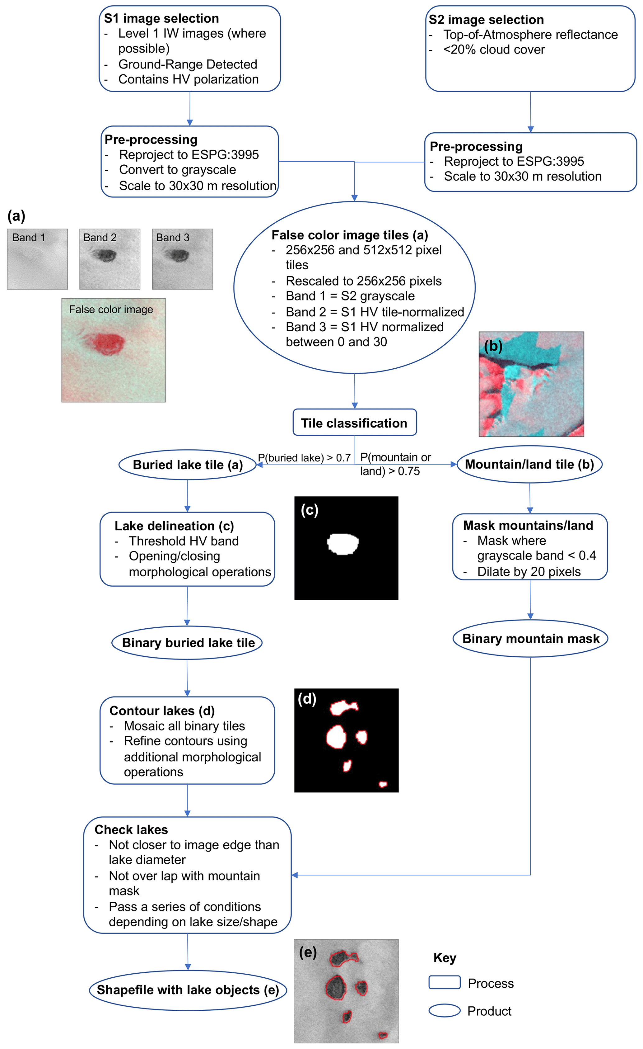
Figure 2 Flow diagram of the methodology with key steps illustrated in image panels (a–e). The final product is shown in (e).

To detect buried lakes across the GrIS, we followed the workflow outlined in Fig. 2. First, we collected S1 and S2 images across the entire periphery of the GrIS for the years 2018 and 2019, and we followed the same data collection and pre-processing steps as outlined above in Sect. 2.1.1. As described above, we used a threshold of 0.7 for buried lake classification such that if an image tile had > 70 % probability of being a buried lake, according to the model, the tile was classified as such.

We also created a mountain/land mask to ensure that mountain areas were not erroneously classified as buried lakes. The mask was created by masking out areas where the grayscale band was <0.4 in image tiles that had >75 % of being either a mountain or land tile, according to the model. The mask was dilated by 20 pixels to include regions of the ice that could have been affected by mountain shadows.

We then used a combination of thresholding and morphological operations to outline individual buried lakes in the image tiles. First, we applied a threshold to band 1 of the false-colour image (normalized HV backscatter from S1) such that all but the darkest 5 % of pixels were masked out. We next performed a series of opening–closing operations using 3×3, 6×6, and finally 12×12 pixel kernels to fill holes in the lake and mask out darker pixels outside the lake. All binary image tiles were then mosaicked, and the individual buried lakes were contoured. We found that repeating this process of thresholding and using morphological operations improved the delineation of buried lakes so these steps were repeated for each contoured area.

Finally, each contoured area had to meet a series of conditions to be considered a buried lake (Appendix Fig. A2). These conditions, which depend on the shape and size of the lake, were optimized by manual inspection to avoid false positives. For example, for smaller buried lakes to be considered, they had to have a lower (compared to larger lakes) microwave backscatter compared to the surrounding background area.

2.2 Surface lake detection

We used all S2 images with <10 % cloud cover, rescaled from the native resolution of 10×10 to 30×30 m resolution (to match S1 image resolution for CNN work and for increased processing speed), from GEE to detect surface lakes across the GrIS during the 2018 and 2019 melt seasons. We followed Williamson et al. (2018a) to mask out clouds by removing pixels in which the band 11 (SWIR) top-of-atmosphere (TOA) reflectance exceeded a threshold of 0.140. To mask ice-marginal areas, we followed Moussavi et al. (2020) by removing pixels with a normalized difference snow index ($\mathrm{NDSI}=\frac{\mathrm{Green}-\mathrm{SWIR}}{\mathrm{Green}+\mathrm{SWIR}})<\mathrm{0.85}$ and where band 2 (blue) <0.4. Pixels above a normalized difference water index ($\mathrm{NDWI}=\frac{\mathrm{Blue}-\mathrm{Red}}{\mathrm{Blue}+\mathrm{Red}}$) threshold of 0.5 (Miles et al., 2017) were considered to be a surface lake pixel. This threshold is higher than that used in other studies (Yang and Smith, 2013; Williamson et al., 2018a; Benedek and Willis, 2021), but we found that using a lower threshold resulted in the erroneous inclusion of cloud and mountain shadows in the analysis. Additionally, use of this higher threshold was appropriate for our goal of comparing relative surface water ponding between the 2018 and 2019 melt seasons in each GrIS subregion. For lakes with small areas of floating surface ice, we filled in these areas by twice performing a morphological closing operation using a 5×5 pixel kernel. We only considered surface lakes that had an area >0.05 km², which is consistent with our area threshold for buried lake detection.

2.3 Buried lake analysis

We compared buried and surface lake elevations by calculating the mean elevation of each lake using the Greenland Ice Mapping Project (GIMP) elevation dataset (Howat et al., 2015). GIMP estimates of surface elevation have an ice-sheet-wide root-mean-square error relative to ICESat elevations of ±10 m above sea level (a.s.l.) ranging from a minimum of ±1 m a.s.l. in most ice areas to ± 30 m a.s.l. in high-relief regions (Howat et al., 2015).

To investigate the buried lake formation process in different regions of the GrIS, we determined the percentage of detected buried lakes in each region that showed any evidence of surface meltwater during the previous summer. We define “evidence of surface meltwater” as the presence of >5 pixels with an NDWI>0.25 within the bounds of the buried lake. For several buried lakes, we also examined a combination of optical imagery from Sentinel-2, Landsat 8, and Landsat 7 from summers dating back to 2012. We also looked at surface topography profiles above select buried lakes using the Arctic DEM Mosaic at 2 m resolution (Porter et al., 2018).

Finally, we compared buried lake distribution with the locations of firn aquifers from 2015–2017 using the Miège (2018) firn aquifer dataset derived from Operation Ice Bridge radar.

2.4 Regional climate model analysis

To relate our buried lake detection results in the 2 consecutive years to the interannual variations in surface climate and surface mass balance, we used output from the regional climate model RACMO2.3_p2 (Noël et al., 2018; RACMO2 hereafter). RACMO2 provides output of Greenland climate and surface mass balance from 1958 to 2020 at 5.5 km horizontal resolution, which is then further statistically downscaled to 1 km horizontal resolution (Noël et al., 2016). We refer the reader to Noël et al. (2018) for a detailed description and evaluation of RACMO2 over the GrIS.

In this study, we analysed RACMO2-derived monthly mean fields of 2 m air temperature, surface melt, precipitation, and surface mass balance for the GrIS from 1 June to 31 December in 2018 and 2019. We also compared these data to the long-term 1958–2017 climatology at elevations <2500 m a.s.l.

2.5 SNOWPACK modelling

To assess meltwater production, percolation, and refreezing in the firn layer in areas with buried meltwater, we used the one-dimensional, physics-based, multi-layer snow cover model SNOWPACK (Lehning et al., 2002b, a). We forced SNOWPACK with RACMO2-derived precipitation, air temperature, relative humidity, incoming longwave and shortwave radiation, and wind speed for the closest grid point to a select buried lake in each of the CW (central west), NW, and NE regions. Simulations were run from January 2000 to December 2019, starting with zero firn layer depth for sites with annual positive mass balance and with 10 m deep ice for sites in the ablation zone.

Within SNOWPACK, the water flow in snow is solved using Richards' equation (Wever et al., 2014), which describes water percolation based on capillarity and hydraulic conductivity. It enables the simulation of water accumulation on microstructural transitions in the snowpack. These transitions can be formed by contrasting microstructural properties (grain size and shape), as well as high variability in hydraulic conductivity (primarily governed by ice content) (Webb et al., 2018). We used the geometric mean to determine hydraulic conductivity at the interface nodes between two layers (Haverkamp and Vauclin, 1979). Using geometric mean maintains strong gradients in conductivity within SNOWPACK, allowing for water accumulation on capillary and hydraulic barriers (Wever et al., 2018).

A zero flux bottom boundary condition was prescribed for temperature, and a free-drainage boundary condition was used for liquid water flow. Other model settings were chosen for optimal simulation of firn on ice sheets following Keenan et al. (2021).

3 Results

3.1 Surface and buried lake detection

We detect a total of 374 buried lakes (covering a total area of 241 km²) following the 2018 melt season (Fig. 3a, Appendix Table B1) and a total of 599 buried lakes (covering 376 km²) following the 2019 melt season (Fig. 3b, Appendix Table B1). In both years, buried lakes are concentrated along the western coast in the SW, CW, and NW regions of the GrIS. Detected buried lakes in SW Greenland have the largest mean area of all regions (0.77 km² following the 2018 melt season, and 0.90 km² following the 2019 melt season) and include the single largest buried lake detected, with an area of 3.95 km² in 2019 (Fig. B2). Buried lakes range in elevation from approximately 455 to 2450 m a.s.l. (Appendix Fig. B3), with the highest buried lakes located in the SW and SE (mean elevations of 1831 and 1710 m a.s.l., respectively) and the lowest buried lakes located in the NE, NO, and NW (mean elevations of 1195, 1135, and 1144 m a.s.l., respectively). These results are broadly consistent with Miles et al. (2017) and Koenig et al. (2015), who found that the majority of buried lakes ranged in elevation from 1000 to 2000 m a.s.l. In general, buried lakes do not appear at substantially different elevations in 2019 than in 2018, with the exception of the NO and NE regions. However, these exceptions may be the result of bias due to a relatively small number of buried lakes detected in 2018 in these regions (4 and 19 buried lakes in the NO and NE regions, respectively).

We also find that the total number of surface lakes and their total areal extent is much lower during the 2018 melt season than during the 2019 melt season. Using our method to detect surface lakes (NDWI > 0.5, and area > 0.05 km²), we detect 3846 surface lakes (covering 1242 km²) in 2018 (Appendix Fig. B1, Appendix Table B2) and 6146 surface lakes (covering 2569 km²) in 2019 (Appendix Fig. B1, Appendix Table B2). Also similar to buried lake distribution, the mean elevation of detected surface lakes is highest in the SW and SE regions (mean 1365 and 1335 m a.s.l., respectively) and lowest in the NO, NW, and NE regions (mean 718, 860, and 962 m a.s.l., respectively). In all regions for both years, the mean elevation of detected buried lakes is higher than for detected surface lakes (Appendix Fig. B3), which is consistent with previous work (Miles et al., 2017; Lampkin et al., 2020).

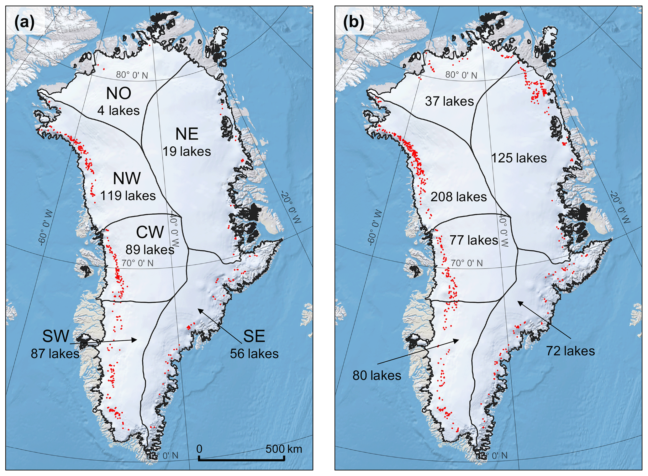
Figure 3 Buried lake distributions, shown in red. (a) The 2018 buried lakes with major GrIS drainage basins labelled (Rignot and Mouginot, 2012). (b) The 2019 buried lakes. The background map is from QGreenland.

On an ice-sheet-wide scale, both the total surface and buried lake extents are much greater in 2019 than in 2018. Regionally, however, different patterns emerge between surface and buried lake distribution for the 2 years. Figure 4a shows that the ratio of surface lake area in 2018 to 2019 is much less than 1 across all GrIS subregions, ranging from 0.32 in NE Greenland to 0.67 in SE Greenland. The 2018:2019 buried lake area ratio, however, varies much more across the six subregions of the GrIS (Fig. 4a). In the SW and CW regions, we find approximately the same 2018 : 2019 buried lake area ratio (0.931 and 0.996, respectively), even though surface lake extent is much less in 2018. In contrast, in the NO and NE regions, the 2018 to 2019 buried lake area ratio is even smaller than the surface lake area ratio (2018:2019 buried lake ratios of 0.133 and 0.171, respectively). The NW and SE regions have comparable 2018:2019 surface and buried lake area ratios. Figure 4b–e show detected buried lakes in NW (b, c) and NE (d, e) Greenland for 2018 and 2019, highlighting the 2019 increase in buried lake area in these regions.

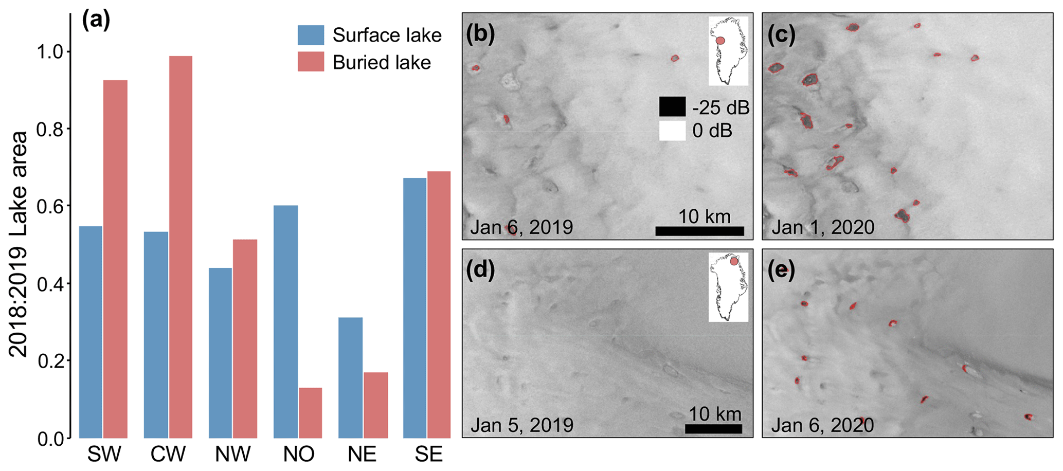
Figure 4 Comparison of 2018 and 2019 total surface and buried lake areas. (a) Ratio of 2018 to 2019 total detected surface (blue) and buried (red) lake area for each major GrIS drainage basin. (b–e) S1 images from NW Greenland (b, c) and NE Greenland (d, e), with detected subsurface lakes outlined in red. (b) 6 January 2019 (following the 2018 melt season). (c) 1 January 2020 (following the 2019 melt season). (d) 5 January 2019. (e) 6 January 2020.

For each buried lake, we additionally analysed select S2 optical imagery from the previous melt season for any evidence of surface water (see Sect. 2.3). Figure 5a shows how the percentage of buried lakes with evidence of liquid water on the surface during the previous melt season varies across the six GrIS subregions. In SW Greenland, most of the detected buried lakes have some surface meltwater within their bounds during the previous melt season (92 % in 2018 and 85 % in 2019). In contrast, very few lakes in the NW (5.9 % in 2018 and 5.8 % in 2019) and SE (1.8 % in 2018 and 4.2 % in 2019) have any evidence of previous summer surface melt within their bounds. This discrepancy indicates that buried lakes may form via different processes in different regions of the GrIS and is something we address further in Sect. 4.3.

Figure 5 The impact of annual precipitation on buried lake formation processes. (a) Percentage of buried lakes that show any evidence of meltwater on the surface (> 5 pixels with an NDWI > 0.25) during the previous melt season, for each of the six subregions. (b) Spatial anomaly of the climatological (1958–2017) mean annual precipitation. Red dots represent buried lakes from 2018 and 2019 that never appeared on the surface during the previous melt season. Blue dots represent detected buried lakes from 2018 and 2019 that appeared on the surface during the previous melt season. (c) Climatological mean annual precipitation with buried lakes plotted in CW Greenland.

Some of the buried lakes in NW and SE Greenland coincide with the locations of, and thus could be connected to, firn aquifers that have been detected in these regions (Fig. 6, Koenig et al., 2014; Forster et al., 2014; Miège et al., 2016; Brangers et al., 2020). It makes sense that these features are co-located because they both require the similar climatic conditions of high melt and high accumulation to exist (Koenig et al., 2014; Munneke et al., 2014; Dunmire et al., 2020). However, firn aquifers, unlike buried lakes, are buried too deep to be directly detected with S1 microwave imagery. The top surface of the perennial firn aquifer in SE Greenland is about 22 ± 7 m below the ice surface (Miège et al., 2016) and can only be detected from S1 images by using the temporal change in microwave backscatter as a proxy to infer the locations of firn aquifers (Brangers et al., 2020). Although it is unclear what relationship the buried lakes and firn aquifers have, we suggest that the buried lakes may feed firn aquifers by draining vertically.

Figure 6 Firn aquifer and detected buried lake locations. (a) The 2015–2017 NW GrIS firn aquifers from Operation Ice Bridge (OIB) (Miège, 2018) and buried lakes following the 2019 melt season. The background image is a S2 image from 1 September 2019. (b) The 2015–2017 SE GrIS firn aquifers from OIB and buried lakes following the 2019 melt season. Background image is a S2 image from 21 July 2019.

3.2 Regional climate model and snow model analysis

To investigate the discrepancies between total surface and buried lake area across the six GrIS subregions, we analysed RACMO2 data from 2018 and 2019 at elevations <2500 m, comparing temperature and melt with the climatological mean (Appendix Figs. B4, B5). We find no spatial or temporal patterns associated with monthly precipitation or surface mass balance anomalies that may explain surface and buried lake differences, so this analysis is not included here. Compared to 2018, 2019 is much warmer across elevations <2500 m in every month from June to November (Fig. B4). During June and July 2019, high monthly mean temperatures are present across the entire ice sheet (+1.52 ^∘C anomaly for June, +1.62 ^∘C anomaly for July). It is likely that these anomalously high temperatures contribute to anomalously high melt during these months (Fig. B5, 1.51 and 1.02 standard deviations higher melt than the climatological mean for June and July, respectively). In contrast, in 2018, June and July have mean temperature anomalies of −0.17 and −1.00 ^∘C, respectively, and lower melt (0.24 and 0.33 standard deviations less than the climatological mean for June and July, respectively). Higher air temperatures in each region during June and July 2019 also contribute to higher ice-sheet-wide July 2019 subsurface temperatures (Fig. 7b). For sites X, Y, and Z, respectively (Fig. 7a), the SNOWPACK-derived mean subsurface temperature in the top 7 m of the snow column is 2.06, 1.97, and 0.34 ^∘C greater in July 2019 than in July 2018. These ice-sheet-wide climatological conditions can explain the greater total surface lake area detected in 2019 compared to 2018 in all six GrIS subregions.

However, from August to November 2019, a different pattern emerges over northern Greenland, marked by anomalously high temperatures and melt compared to the rest of the continent and to 2018. In the NW, NO, and NE regions collectively, the 2019 temperature anomalies for areas <2500 m are +1.17, +1.38, +1.96, and +2.00 ^∘C for August, September, October, and November, respectively. The August 2019 melt is 2.26 standard deviations higher than the climatological mean (compared to only 0.26 standard deviations higher in August 2018). In comparison, in the CW, SW, and SE regions, the 2019 temperature anomalies for these same months are much less remarkable at −0.20, +0.26, +0.51, and +1.60^∘C, and the August 2019 melt anomaly was only 0.52 standard deviations higher than the climatological mean. Higher air temperatures in NW, NO, and NE Greenland from August–November 2019 lead to correspondingly higher subsurface firn temperatures than in 2018 in these regions in the SNOWPACK simulations (Fig. 7b). For example, at site Z in NE Greenland, the September 2018 and 2019 temperature anomalies are −2.54 and +4.04 ^∘C, respectively, and the mean September simulated subsurface temperature in the top 7 m of the snow column is 3.18 ^∘C warmer in 2019 than in 2018. In contrast, at site X in CW Greenland, the September 2018 and 2019 temperature anomalies are −0.71 and +0.98 ^∘C, respectively, and the mean September simulated subsurface temperature in the top 7 m of the snow column is 0.80 ^∘C colder in 2019 than in 2018. SNOWPACK analysis at site Y located in NW Greenland shows that meltwater existed in the subsurface during both the 2018 and 2019 melt seasons, freezing through entirely in 2018 but lasting through the end of the year in 2019 (Fig. 7c).

These results suggest that for the three regions in northern Greenland (NW, NO, and NE), anomalously high autumn air temperatures lead to increased subsurface firn temperatures, delaying and decreasing subsurface meltwater freeze-through in 2019. This, combined with higher northern Greenland melt in the late summer of 2019, may contribute to the higher total buried lake area detected in NW, NO, and NW Greenland in 2019 compared to elsewhere on the GrIS.

Figure 7 Air and subsurface firn temperature modelling analysis. (a) The 2018 to 2019 mean monthly temperature difference for July, August, September, and October from left to right. Areas with temperature anomalies that are significantly different from the climatology at the 95 % confidence level are shaded with a cross-hatch pattern. (b) Subsurface firn temperature profiles at sites X (CW Greenland), Y (NE Greenland), and Z (NW Greenland) for July, August, September, and October from left to right. (c) Subsurface firn temperature profiles at site Z (NW Greenland).

4 Discussion

4.1 Buried lake detection limitations

The number of buried lakes detected in this study is likely an underestimation of the actual number of buried lakes that existed across the GrIS in 2018 and 2019 for several reasons. Firstly, our detection of buried lakes was dependent on prescribed thresholds based on the microwave backscatter within the buried lake bounds relative to the surrounding area (Appendix Fig. A2). We set these thresholds in a conservative manner that prioritized minimizing false positives, but as a result, our analysis likely missed some buried lakes that do not meet our thresholds. For example, if we increased the thresholds we use in this study by 5 % (which makes the result less conservative), we saw 5.2 % and 5.0 % increases in the total detected buried lake volume in 2018 and 2019, respectively. However, this changed the 2018:2019 buried lake area ratio by only +0.18 %. Conversely, a 5 % decrease in the thresholds we use in this study (which makes the results even more conservative) resulted in 11.0 % and 5.4 % decreases in the total detected buried lake volume in 2018 and 2019, respectively. This decreased the 2018:2019 buried lake area ratio by 5.8 %, indicating that the difference in backscatter between a buried lake and its surroundings was greater in 2018 than it was in 2019. A possible explanation for this is that the buried lakes detected in 2018 had persisted from the 2017 melt season or before, resulting in these lakes being buried at greater depths than the lakes that formed after the 2019 melt season. Another possible explanation is that buried lakes contained less water in 2018 than in 2019, making the lakes in 2018 appear less different relative to their surrounding regions in the S1 images.

Another reason why our method may underestimate the number of buried lakes is because we do not consider lakes that are smaller than 0.05 km² (approximately 56 pixels), so our analysis may have missed smaller buried lakes. Additionally, as the penetration depth of C-band microwave radar in ice and snow is only several metres (Rignot et al., 2001), buried lakes located at depths greater than this will not be detected using our method. Finally, recent work has shown that buried lakes can drain, and on very rare occasions even during the winter months (Benedek and Willis, 2021); though this process will likely only contribute a very minor source of error.

4.2 Buried lake formation processes

Previous studies have generally assumed that buried lakes on the GrIS develop when a surface lake partially freezes through and then gets buried by snowfall, insulating any remaining liquid water under the surface (Koenig et al., 2015; Schröder et al., 2020). Modelling efforts have confirmed that this process is sufficient to allow liquid water to exist under the ice surface throughout the winter on both the Greenland and Antarctic ice sheets (Law et al., 2020; Dunmire et al., 2020; Lampkin et al., 2020). In SW Greenland, most of the buried lakes that we detected had some surface meltwater within their bounds during the previous melt season (Fig. 5), supporting the hypothesis that buried lakes form due to surface lake freeze-over followed by insulating snowfall and indicating that this is the dominant process through which buried lakes form in SW Greenland. This process is illustrated by a series of chronological satellite images of a buried lake detected following the 2019 melt season (Fig. 8).

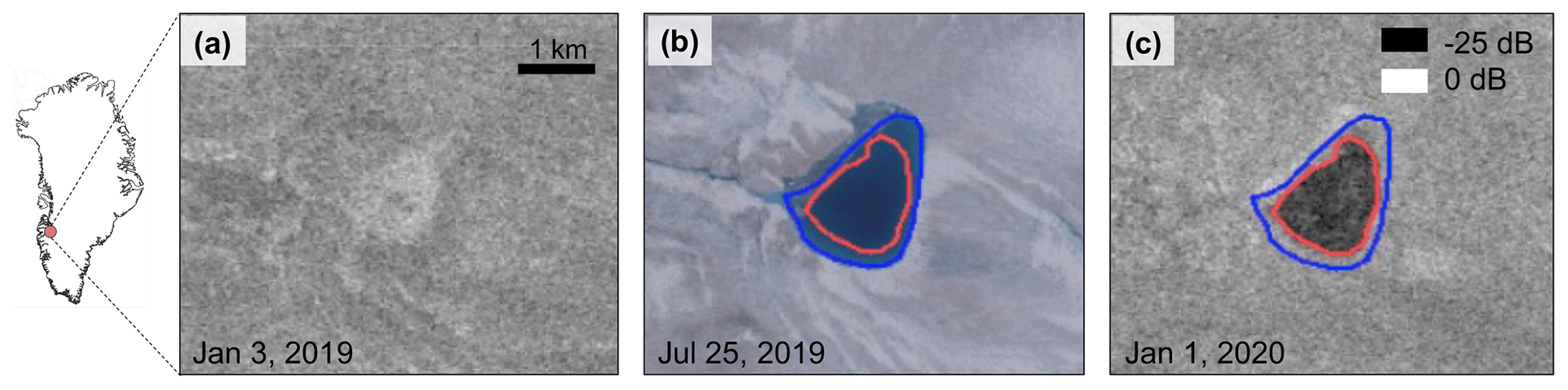
Figure 8 Chronological S1 (greyscale) and S2 (true colour) images of a buried lake detected in SW Greenland in the winter following the 2019 melt season. (a) S1 image from 3 January 2019 with no buried lake detected. (b) S2 image from 25 July 2019 with surface lake extent outlined in blue and post-melt season buried lake extent outlined in red. (c) S1 image from 1 January 2020.

However, in NW and SE Greenland, very few of the detected buried lakes had any evidence of previous summer surface melt within their bounds; suggesting that buried lakes in these two regions tend to form without prior surface ponding (Fig. 9). These results indicate that buried lakes in SE and NW Greenland may form via a different process than elsewhere on the GrIS. One likely alternative explanation is that near-surface meltwater percolates downward and collects in depressions on impermeable ice layers, which are co-located with surface topological depressions (Drews et al., 2020). These subsurface ice layers could be the result of thermally controlled refreezing of downward-percolating meltwater, providing impermeable layers for future meltwater to collect on top of. Evidence in support of this idea is that many of the buried lakes in the NW and SE are found to be located directly below surface depressions (Fig. 9e, j, k). Our SNOWPACK model simulations further support this idea. For example, Fig. 7c shows that meltwater accumulates on subsurface ice layers with low hydraulic conductivity. The simulated water content reaches up to 40 %–50 % in some subsurface layers, indicating the formation of slush and subsequent pore space depletion. Substantial energy loss is required to refreeze slush layers, and autumn snowfall slows this refreezing process (e.g. compare autumn 2018 and 2019 in Fig. 7c). We also find that in autumn and winter, subsurface meltwater refreezing thickens the low-permeability ice slabs, above which future meltwater may accumulate.

A second possible explanation for how buried lakes can form without initial surface meltwater is via penetration and absorption of shortwave solar radiation through the snowpack, which is capable of creating layers of slush and liquid water beneath the surface (Leppäranta et al., 2013; MacAyeal et al., 2019) without the presence of surface water. This is found to occur particularly when the surface is formed by pure ice. While downward percolation of meltwater is the more likely explanation for buried lake formation without the presence of surface meltwater in areas with a firn layer, subsurface penetration of solar radiation may enhance melting in the vicinity of pre-existing buried lakes (Dunmire et al., 2020).

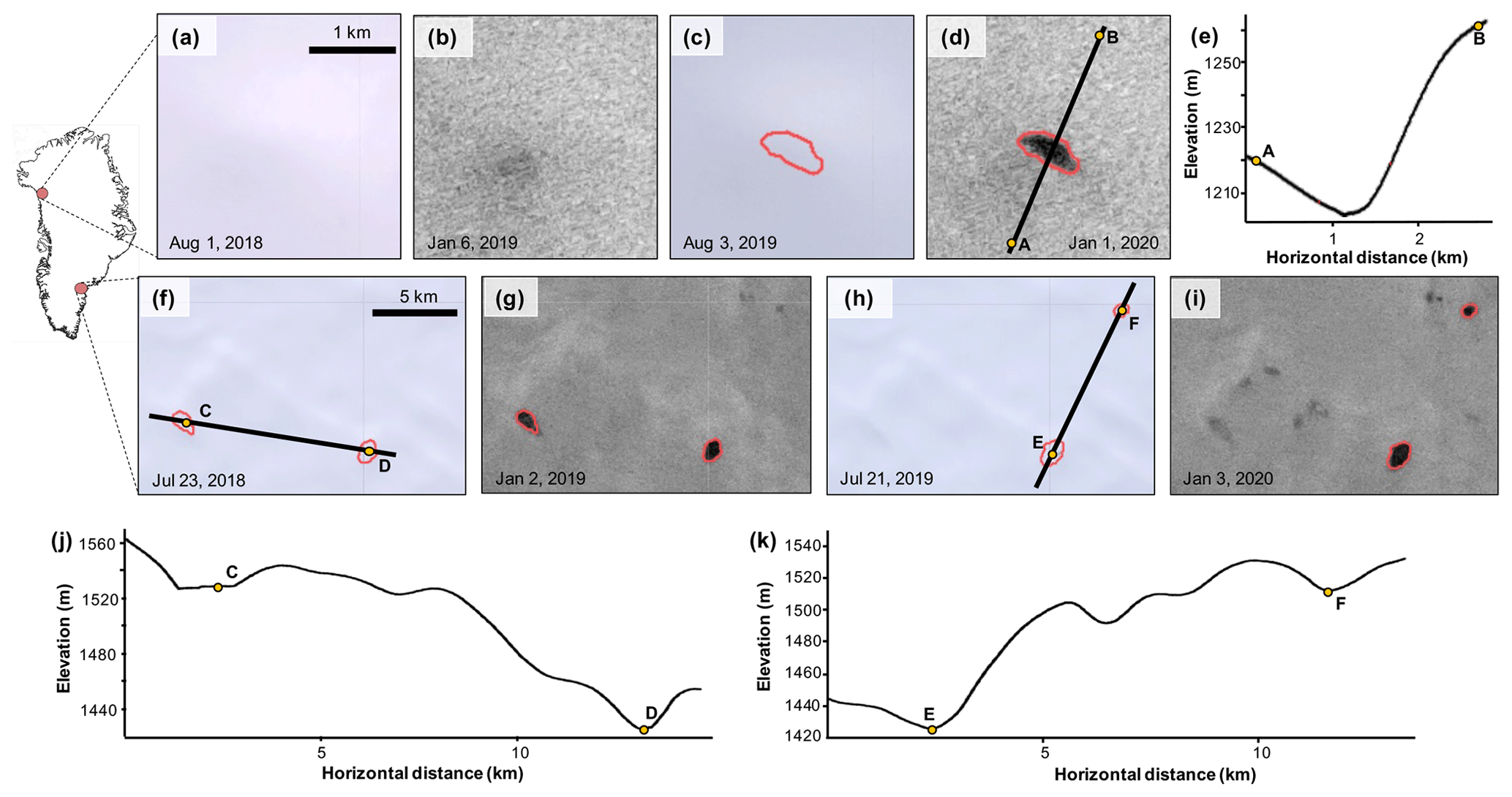
Figure 9 Optical and microwave images and surface elevation profiles of buried lakes in NW Greenland (a–e) and SE Greenland (f–i) in chronological order. (a) S2 image from 1 August 2018. (b) S1 image from 6 January 2019. (c) S2 image from 3 August 2019 with post-2019 melt season buried lakes outlined in red. (d) S2 image from 1 January 2020. (e) Surface elevation profile from Arctic DEM Mosaic (Porter et al., 2018) over the buried lake shown in (d). (f) S2 image from 23 July 2018 with post-2018 melt season buried lakes outlined in red. (g) S1 image from 2 January 2019. (h) S2 image from 21 July 2019 with post-2019 buried lakes outlined in red. (i) S1 image from 3 January 2020. (j) Surface elevation profile from ArcticDEM Mosaic over buried lakes C and D detected following the 2018 melt season. (k) Surface elevation profile from ArcticDEM Mosaic over buried lakes E and F detected following the 2019 melt season.

While Fig. 5 indicates that the dominant buried lake formation process is different in different regions of the GrIS, it is likely that a combination of formation mechanisms exist in each region. Further, in some cases, it appears that a combination of formation processes even exist for individual lakes. For example, Fig. 10 includes a series of images of a buried lake detected in CW Greenland. S1 and S2 imagery show that the areal extent of the buried lake is greater than the surface lake detected during the previous melt season. These images therefore suggest that the formation of this buried lake resulted not only from the burial of a surface lake by snowfall, but also due subsurface melting and/or the downward percolation of surface meltwater.

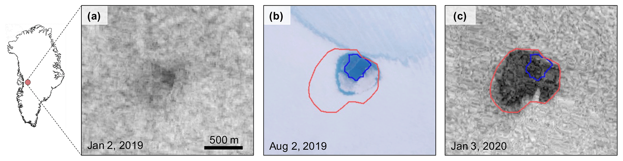
Figure 10 Chronological optical and microwave images of a buried lake in CW Greenland. (a) S1 image from 2 January 2019. (b) S2 image from 2 August 2019 with detected surface lakes outlined in blue and detected post-2019 melt season buried lakes outlined in red. (c) S1 image from 3 January 2019.

We hypothesize that the dominant formation mechanism in different regions of the GrIS is driven by, in part, regional differences in annual precipitation. Generally, buried lakes that appear on the surface during the previous melt season are located in areas with relatively lower total annual precipitation (Fig. 5b). Conversely, large concentrations of buried lakes that never appear on the surface during the previous melt season are located in areas with relatively higher total annual precipitation. For example, in CW Greenland (Fig. 5c), the 1958–2017 climatological average annual precipitation that falls over the buried lakes detected in both 2018 and 2019 is 509 mm w.e. per year for buried lakes which never appear on the surface during the previous melt season and 451 mm w.e. per year for buried lakes which do appear on the surface during the previous melt season. The difference in these two means is statistically significant at the 99 % confidence level.

The observations described above therefore suggest that a mechanism by which annual precipitation may impact the buried lake formation process is through the availability of near-surface porous firn (Fig. B6). In areas with relatively low annual precipitation, there is less near-surface porous firn for meltwater to percolate, leading to increased surface ponding, and potentially a greater proportion of buried lakes that form following surface pond burial relative to other regions. In contrast, in areas with relatively high precipitation, there is more near-surface firn available to store meltwater, which may initially pool on subsurface impermeable ice layers, leading to less surface ponding prior to buried lake detection.

4.3 Climate drivers of buried lake distribution

Using a regional climate model to analyse temperature and melt anomalies from 2018 and 2019, we show that an increase in buried lake area in 2019 in northern Greenland (NW, NO, and NE regions) is likely due to a combination of anomalously high late-season melt and anomalously high near-surface autumn (i.e. August to November) air temperatures. Warmer late-summer and autumn air temperatures may prevent the water in surface lakes from freezing entirely and allow some liquid meltwater to remain buried. This analysis suggests that increasing air temperatures, which contribute to increased summer melt, will likely lead to an increase in the number and area of buried lakes and therefore an increased volume of liquid water that is stored beneath the surface during the winter. Surface lake distribution across the GrIS has expanded inland to higher elevations (Howat et al., 2013), and it is expected that surface lakes will continue to form at higher elevations as air temperatures continue to rise in the future (Leeson et al., 2015). Thus, we also expect that buried lakes will form further inland at higher elevations in a warming climate, with potential implications for changing surface hydrology and total ice loss.

4.4 Buried lake implications

Perennial buried lakes store meltwater that could otherwise run off and eventually drain into the ocean. Thus, these features act as a potential buffer against sea level rise. However, this buffer may only be temporary given that buried lakes have been shown to drain (Dunmire et al., 2020), even occasionally during the winter (Benedek and Willis, 2021). Because buried lakes exist perennially and can drain throughout the year, at lower elevations (<1600 m; Poinar et al., 2015), drainage of buried lakes could provide an influx of water to the bedrock at atypical times of year. However, as only a small fraction of buried lakes drain during the winter, the influx of meltwater to the bedrock during winter months is likely to be minimal. Additionally, as some buried lakes in the SE and NW regions of the GrIS are located directly above observed firn aquifers, their potential drainage could provide an influx of meltwater to these firn aquifers. However, as the volume of water stored in buried lakes on an ice-sheet-wide scale is likely to be relatively small, these effects would mainly be relevant at local scales, particularly where large concentrations of buried lakes exist.

5 Conclusions

In this paper, we have developed a method that uses a convolutional neural network to detect buried lakes across the entire GrIS following each of the 2018 and 2019 melt seasons. We compared buried and surface lake spatial distributions across six GrIS subregions and used a regional climate model to explain the spatial and temporal differences. We find that while the total surface lake areal extent was less in 2018 than in 2019 across all six subregions, buried lake extent is roughly equal in 2018 and 2019 in the SW and CW regions but much less in 2018 in the NO and NE regions. These regional differences in buried lake extent between 2018 and 2019 can be explained by regional patterns of late-summer (August) melt and autumn (September–November) air temperatures. Anomalously high late-summer melt, coupled with anomalously high autumn air temperatures in 2019 in northern Greenland likely contributed to increased buried lake extent in this region following the 2019 melt season. Additionally, simulations using the one-dimensional SNOWPACK model confirm that subsurface meltwater in buried lakes remained unfrozen through autumn 2019.

We also examined the buried lake formation process by investigating S1 and S2 imagery prior to the detection of buried lake features. We find that different formation processes likely occur in different regions. In SW and CW Greenland, buried lakes likely form when surface lakes partially freeze over and become insulated by following snowfall. In contrast, in SE and NW Greenland, no evidence of surface melt exists in optical imagery prior to the discovery of the majority of detected buried lakes; indicating that these features form via a different process. It is possible that subsurface penetration of shortwave radiation, and/or downward percolation and subsurface pooling of near-surface melt, could be responsible for the formation of buried lakes in SE and NW Greenland. The simulation of the firn in NW Greenland showed liquid water accumulating on low-permeability ice layers approximately 2 m below the surface.

Surface meltwater on the GrIS plays an important role in both ice sheet dynamics, as lake drainage events provide an influx of meltwater to the bed which may temporarily increase ice velocity and direct mass loss, as meltwater runoff positively contributes to sea level rise. The evolution of surface meltwater features has been thoroughly examined in prior studies using optical satellite imagery. In contrast, buried meltwater features are invisible in optical imagery, and as a result, these features are more poorly understood than their surface counterparts. Here, we provide a method for continent-wide mapping of buried lakes and a comprehensive look at the drivers of their formation and distribution across the GrIS.

Appendix A: Additional tables/figures relating to methods

Krizhevsky et al. (2012)Huang et al. (2017)Szegedy et al. (2015)Tan et al. (2019)Sandler et al. (2018)He et al. (2016)Ma et al. (2018)Simonyan and Zisserman (2015)

Table A1 Comparison of model evaluation metrics between different CNN architectures.

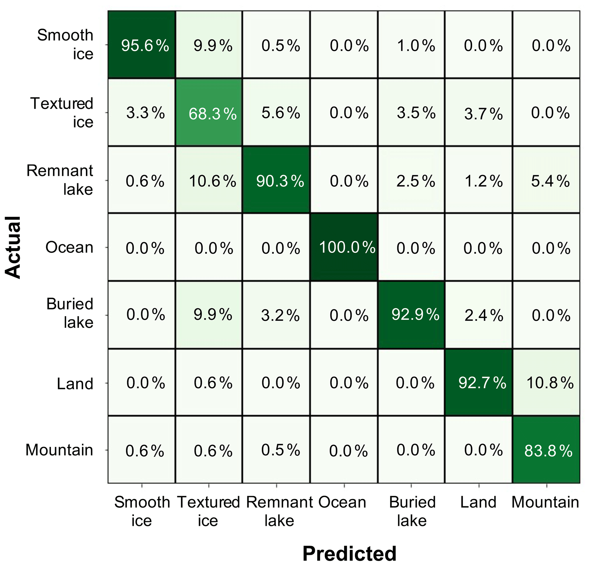
Figure A1 CNN test dataset confusion matrix. Values are normalized by the predicted conditions and thus represent the precision for each class. For example, a value of 92.9 % for predicted shows a buried lake and actual show a buried lake, meaning that 92.9 % of the predicted buried lakes are actually buried lakes.

Figure A2 Thresholds used in the CNN for different buried lake shapes/sizes.

Appendix B: Additional tables/figures relating to results

Table B1 Detected buried lake statistics.

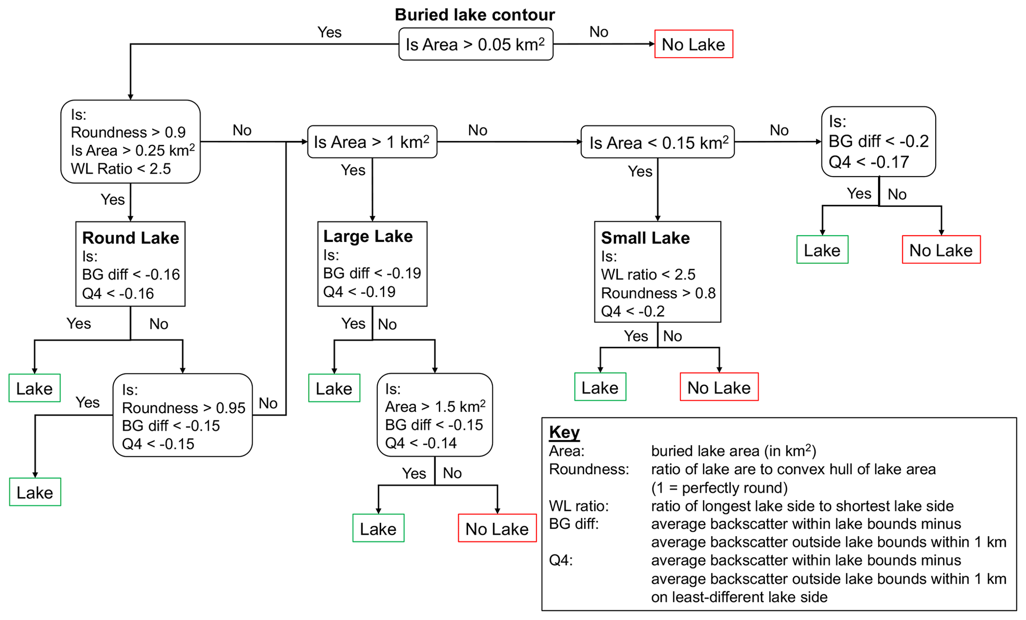
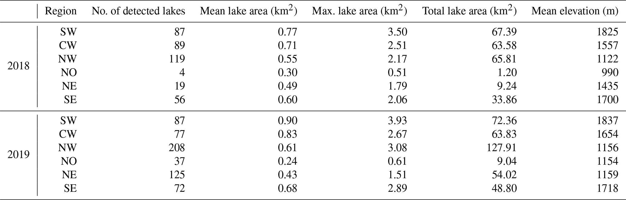
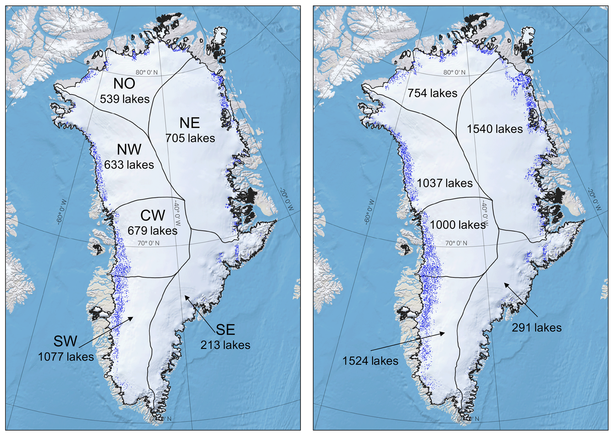
Figure B1 Surface lake distributions, shown in blue. (a) The 2018 detected surface lakes with major GrIS drainage basins labelled (Rignot and Mouginot, 2012). (b) The 2019 detected surface lakes. The background map is from GEE (Gorelick et al., 2017).

Table B2 Detected surface lake statistics.

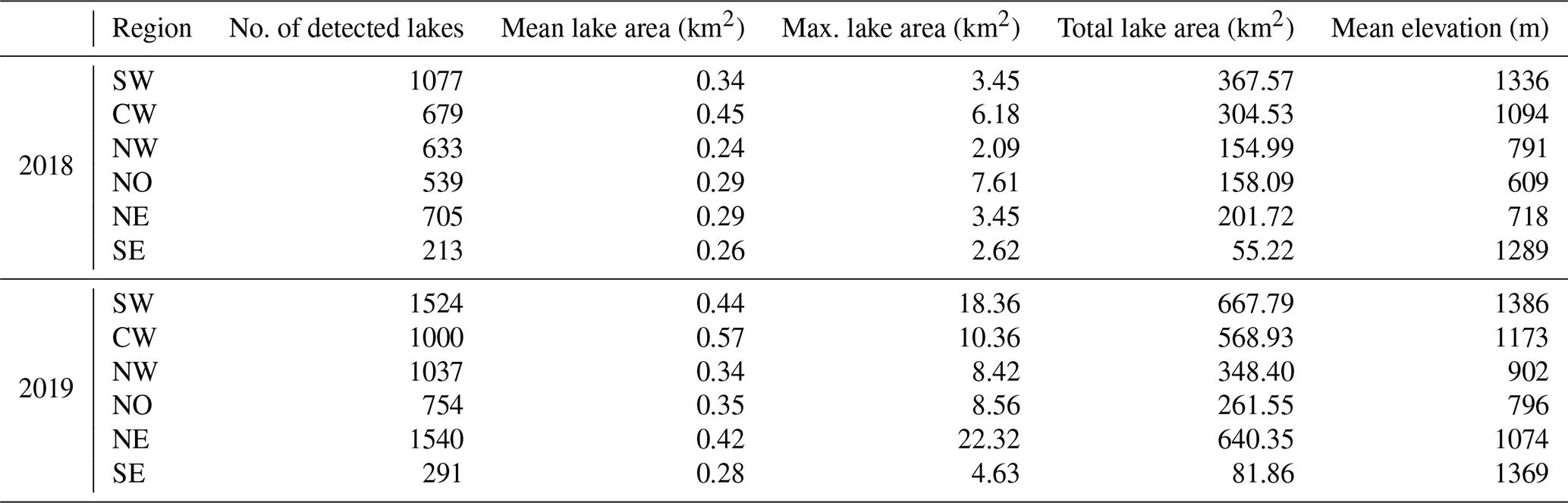
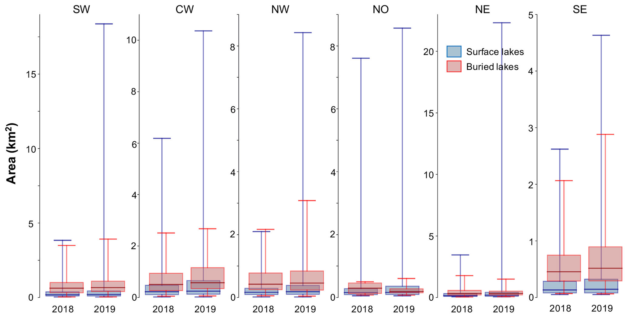
Figure B2 Box plots showing the distribution of detected buried (red) and surface (blue) lake area in each of the six GrIS subregions. Boxes represent the interquartile range of lake area, and whiskers represent the entire range of lake area in a given region/year.

Figure B3 Box plots showing the distribution of detected buried (red) and surface (blue) lake elevations in each of the six GrIS subregions. Boxes represent the interquartile range of lake elevations, and whiskers represent the entire range of lake elevation in a given region/year.

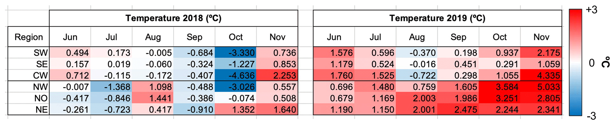
Figure B4 June through November monthly temperature anomalies below 2500 m (^∘C) from the 1958–2017 mean climatology for each subregion of the GrIS in 2018 and 2019.

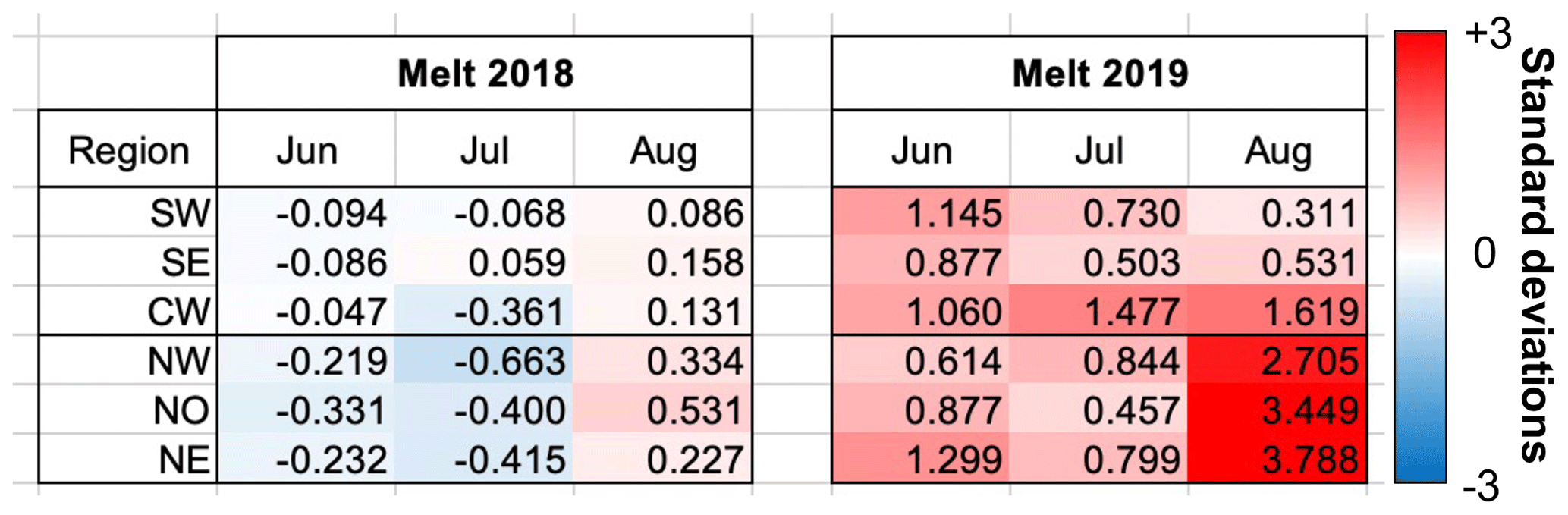
Figure B5 June, July, and August monthly melt anomalies below 2500 m from the 1958–2017 mean climatology for each subregion of the GrIS in 2018 and 2019.

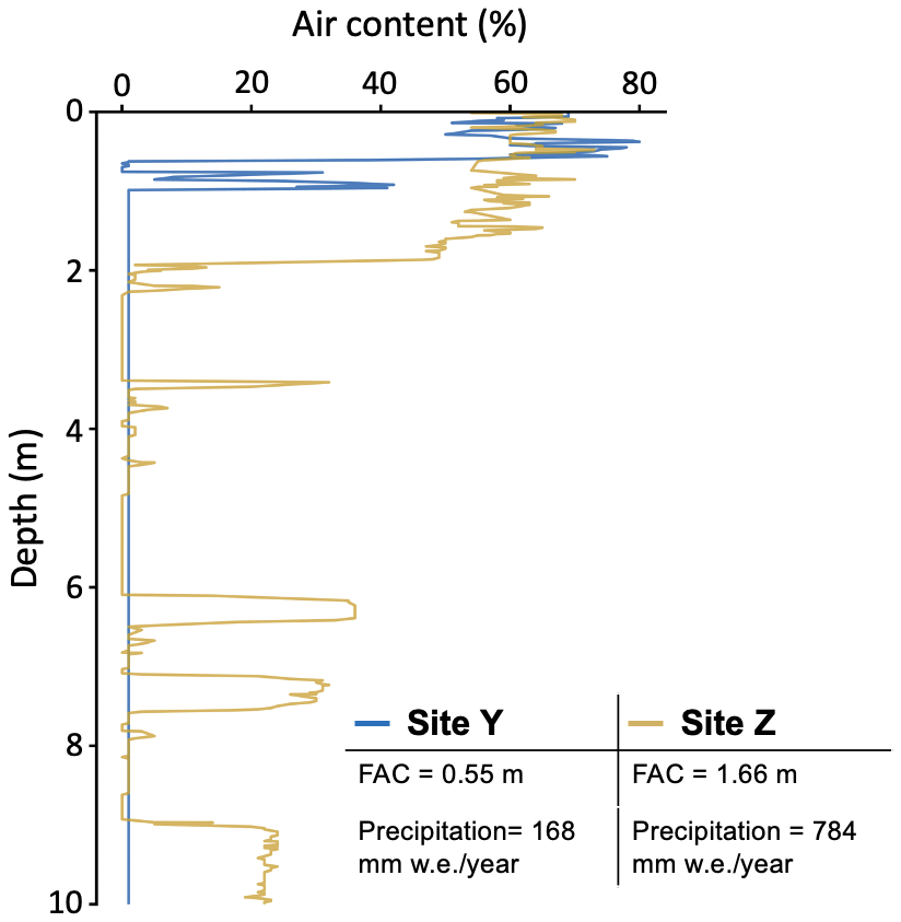
Figure B6 Simulated air content profiles at sites Y and Z. Firn air content (FAC) in the top 10 m and total annual precipitation from the RACMO 1958–2017 climatology for each site are noted in the table.