the Creative Commons Attribution 4.0 License.
the Creative Commons Attribution 4.0 License.
 | 20 Jan 2021
Passive seismic recording of cryoseisms in Adventdalen, Svalbard
Alfred Hanssen
Bent Ole Ruud
Helene Meling Stemland
Tor Arne Johansen
A series of transient seismic events were discovered in passive seismic recordings from 2-D geophone arrays deployed at a frost polygon site in Adventdalen, Svalbard. These events contain a high proportion of surface wave energy and produce high-quality dispersion images using an apparent offset re-sorting and inter-trace delay minimisation technique to locate the seismic source, followed by cross-correlation beamforming dispersion imaging. The dispersion images are highly analogous to surface wave studies of pavements and display a complex multimodal dispersion pattern. Supported by theoretical modelling based on a highly simplified arrangement of horizontal layers, we infer that a ∼3.5–4.5 m thick, stiff, high-velocity layer overlies a ∼30 m thick layer that is significantly softer and slower at our study site. Based on previous studies we link the upper layer with syngenetic ground ice formed in aeolian sediments, while the underlying layer is linked to epigenetic permafrost in marine-deltaic sediments containing unfrozen saline pore water. Comparing events from spring and autumn indicates that temporal variation can be resolved via passive seismic monitoring. The transient seismic events that we record occur during periods of rapidly changing air temperature. This correlation, along with the spatial clustering along the elevated river terrace in a known frost polygon, ice-wedge area and the high proportion of surface wave energy, constitutes the primary evidence for us to interpret these events as frost quakes, a class of cryoseism. In this study we have proved the concept of passive seismic monitoring of permafrost in Adventdalen, Svalbard.
- Article
(15374 KB) - Full-text XML
- BibTeX
- EndNote


Permafrost is defined as ground that remains at or below 0 ∘C for at least 2 consecutive years (French, 2017). On Svalbard, an archipelago located in the climatic polar tundra zone (Kottek et al., 2006), at least 90 % of the land surface area not covered by glaciers is underlain by laterally continuous permafrost (Christiansen et al., 2010; Humlum et al., 2003). A seasonally active layer, where freezing/thawing occurs each winter/summer, extends from the surface to a depth of 0.8–1.2 m (Christiansen et al., 2010) and overlies the permafrost. However, the purely thermal definition of permafrost means that the mechanical properties can vary widely depending on the actual ground-ice content. The ground-ice content varies spatially according to sediment texture, organic content, moisture availability and sediment accumulation rate (Gilbert et al., 2016; Kanevskiy et al., 2011; O'Neill and Burn, 2012). Because of the significant impact of ice content on mechanical strength, seismic velocities are a relatively sensitive tool to study the subsurface distribution of ground ice (Dou et al., 2017; Johansen et al., 2003).
The thermal dynamics of this permafrost environment lead to an interesting phenomenon called cryoseisms, sometimes referred to as frost quakes. Cryoseisms are produced by the sudden cracking of frozen material at the Earth's surface (Battaglia and Chagnon, 2016). They are typically observed in conjunction with abrupt drops in air and ground temperature below the freezing point, in the absence of an insulating snow layer and in areas where high water saturation is present in the ground (Barosh, 2000; Battaglia and Chagnon, 2016; Matsuoka et al., 2018; Nikonov, 2010). When the surface temperature drops well below 0 ∘C the frozen permeable soil expands, increasing the stress on its surroundings, which can eventually lead to explosive pressure release and tensional fracturing (Barosh, 2000; Battaglia and Chagnon, 2016). Seismic waves from these events decay rapidly with distance from the point of rupture but have been felt at distances of several hundred metres to several kilometres and are usually accompanied by cracking or booming noises, resembling falling trees, gunshots or underground thunder (Leung et al., 2017; Nikonov, 2010). The zero focal depth of cryoseisms means that, relative to tectonic earthquakes, a larger proportion of the energy is distributed in the form of surface waves (Barosh, 2000).
Methods based on the analysis of surface waves are used extensively in engineering fields, such as the non-destructive testing of structures or assessment of the mechanical properties of soils relating to their use as a foundation for built structures (Chillara and Lissenden, 2015; Park et al., 1999, 2007; Rose, 2004). In a typical soil profile, the shear velocity and stiffness of the ground increase gradually with depth due to compaction, leading to a simple wave field dominated by fundamental mode Rayleigh waves (Foti et al., 2018). Mechanical properties of the ground are then estimated relatively simply from the geometrical dispersion of the recorded wave field, i.e. the measured pattern of phase velocity as a function of frequency, where lower frequencies interact with the ground to greater depths than higher frequencies.
By contrast, in permafrost environments, the surface layer freezes solidly during the winter, leading to an increase in the shear modulus of the upper layer (Johansen et al., 2003) and an inverse shear velocity with depth profile. This is similar to the case of pavement in civil engineering studies, where a thin, relatively stiff, high-velocity layer at the surface overlies softer and slower ground materials beneath. The high-velocity surface layer acts as a waveguide, permitting the excitation of higher-order wave modes, and the wave field becomes significantly more complicated due to the large number of simultaneously propagating wave modes (Foti et al., 2018; Ryden and Lowe, 2004). Such engineering applications have furthermore driven the development of wave propagation models capable of modelling these complicated wave fields. For example, the ground may be represented by a horizontally layered medium with partial wave balance at the interfaces, for which the dispersion spectrum and stress-displacement field is readily calculated using the global matrix method (Lowe, 1995).
Our study site is located in Adventdalen, near the main settlement Longyearbyen on the island Spitsbergen, within the Svalbard archipelago in the high Arctic, as shown in Fig. 1. The climate of this area, as recorded at Longyearbyen airport, is characterised by low mean annual precipitation of 192 mm and mean annual air temperature of −5.1 ∘C for the period 1990–2004, rising to −2.6 ∘C during the period 2005–2017. The maritime setting and alternating influence of low-pressure systems from the south and polar high-pressure systems means that rapid temperature swings are common during winter from above 0 ∘C down to −20 or −30 ∘C, while summer temperatures are more stable in the range of 5–8 ∘C (Matsuoka et al., 2018). Snow cover in the study area is typically shallow, due to the strong winds that blow along the valley, and varies according to local topography with 0–0.1 m over local ridges and 0.3–0.4 m in troughs. Positive temperature and snowmelt events also occur sporadically through the freezing season (October to May) and subsequently result in the formation of a thin ice cover. Both shallow snow cover and thin ice cover permit efficient ground cooling throughout the freezing season (Matsuoka et al., 2018).
Adventdalen has continuous permafrost extending down to ∼100 m depth (Humlum et al., 2003), but the highest ground-ice content is restricted to the uppermost ∼4 m in the loess-covered river terraces that bound the relatively flat, braided Adventelva river plain. The geological setting of the study site is illustrated in Fig. 2. The formation of permafrost in Adventdalen began around 3 ka, concurrent with the subaerial exposure and onset of aeolian sedimentation on valley-side alluvial terraces (Gilbert et al., 2018). Sediment cores studied by Cable et al. (2018) and Gilbert et al. (2018) show a consistent pattern of an increased ground-ice content over a ∼4 m thick interval (decreasing towards the coast), beneath a ∼1 m thick active layer. This interval was observed consistently in cores retrieved from alluvial and loess deposits and is interpreted as ice-rich syngenetic permafrost (Cable et al., 2018; Gilbert et al., 2018).
The underlying interval consists of marine-influenced deltaic sediments into which permafrost has grown epigenetically and where ground-ice content remains low (Gilbert et al., 2018). Unfrozen permafrost has been mapped in Adventdalen below the Holocene marine limit (which includes the entire study area as illustrated in Fig. 1) using nuclear magnetic resonance and controlled source audio-magnetotelluric data (Keating et al., 2018). This is again related to the presence of saline pore water in these marine-influenced deltaic sediments that causes the pore water to remain at least partially unfrozen despite sub-zero temperatures.
Ice-wedge polygons, one of the most recognisable landforms in permafrost environments (Christiansen et al., 2016), are present at the investigated site in Adventdalen. They form when freezing winter temperatures cause the ground to contract and crack under stress (Lachenbruch, 1962). Water later infiltrates the cracks and refreezes as thin ice veins that extend down into the permafrost. These veins have lower tensile strength compared to the surrounding ground (Lachenbruch, 1962; Mackay, 1984), so subsequent freeze-induced cracking occurs preferentially along this plane of weakness. The repeated cracking, infilling and refreezing causes the ice wedges to grow laterally, forcing the displaced ground upwards and resulting in a series of ridges in a polygonal arrangement that are the surface hallmark of the phenomenon (Christiansen et al., 2016; Lachenbruch, 1962).
Sudden ground accelerations corresponding to cryoseismic events have previously been observed at our study site in Adventdalen. Matsuoka et al. (2018) monitored three ice-wedge troughs within an area of polygonal patterned ground at the site, using a combination of extensometers, accelerometers and breaking cables connected to timing devices. Their study, which extended over the 12-year period 2005–2017, provides a valuable overview of the seasonality and correspondence between ground motion and environmental parameters. The related study of O'Neill and Christiansen (2018) further details the accelerometer results. Ice-wedge cracking was typically registered in late winter, when the top of the permafrost cooled to around −10 ∘C, resulting in large accelerations of 5 g to more than 100 g. However, O'Neill and Christiansen (2018) also report smaller magnitude accelerations throughout the freezing season, typically in conjunction with rapid surface cooling, that are thought to be caused by the initiation of cracks within the active layer or the horizontal and vertical propagation of existing ice-wedge cracks. Given the timing of the field campaigns for the present study, during spring and autumn of 2019, we expect it is rather the latter category of events that have been recorded.
In the present study ground motion was recorded using geophones deployed in 2-D arrays (the geometry of which is discussed in Sect. 3.3.1). During the spring field campaign, groups of eight gimballed vertical-component geophones connected in series (geophone type sensor SM-4/B 14 Hz, 0.7 damping and spurious frequency of 190 Hz) were deployed on the snow surface at each receiver location. During deployment for the autumn field campaign, geophones were embedded into the unfrozen ground surface as an assortment of spike geophones (Sercel SG-10 10 Hz) connected in series in strings of four geophones and 3C geophones (DT-Solo 3C with z element HP301V 10 Hz) where only the vertical channel was used. Both of these geophone types have damping of 0.7, giving a flat response above the natural frequency up to the spurious frequency of 240 Hz. Data were recorded for defined time intervals as will be discussed in Sect. 4.1, mandated primarily by battery considerations.
In this study, we present a methodology to isolate transient seismic signals in passive seismic recordings from two-dimensional vertical-component geophone arrays. These transient signals contain surface wave energy with a relatively high signal-to-noise ratio. We implement a novel method to localise the unknown source position of these signals based on the 2-D receiver array geometry and subsequently recover dispersion spectra using a cross-correlation beamforming technique. In order to infer subsurface physical properties we generate theoretical dispersion curves using the global matrix method (Lowe, 1995) based on idealised horizontally layered media models. The forward model is manually tuned to achieve the best fit with the experimentally observed dispersion spectra. Similar experiments were conducted over two field campaigns in the spring and autumn in order to investigate temporal variation in permafrost mechanical strength.
3.1 Isolation of microseismic events in passive records
Our passive seismic recordings contain a significant amount of non-surface wave energy, including wind noise and air waves. As a result we find it more effective to isolate and analyse specific transient microseismic events rather than attempting to recover the Green's function from ambient noise cross-correlations as for example Sergeant et al. (2020) have done for passive recordings on glaciers. The periodic microseismic signals are isolated from background random noise based on permutation entropy, a nonlinear statistical measure of randomness in a time series (Bandt and Pompe, 2002), that produces local minima for coherent signals embedded in noise. We follow the implementation of Unakafova and Keller (2013) using ordinal patterns of third order extracted over successive samples and a sliding window size of 200 samples. We then apply a peak-finding algorithm to identify local minima in permutation entropy that meet peak prominence criteria defined by thresholds of peak value, height and width. An example of event detection is shown in Fig. 3 for real, noisy data recorded at the study site.

Figure 11:100 000 scale map showing the location of the study area (red box) in Adventdalen. Inset map illustrates the location with respect to the Svalbard archipelago. The Holocene marine limit (red dashed line) is drawn according to Lønne (2005). Map data © Norwegian Polar Institute (http://npolar.no, last access: 3 September 2020).
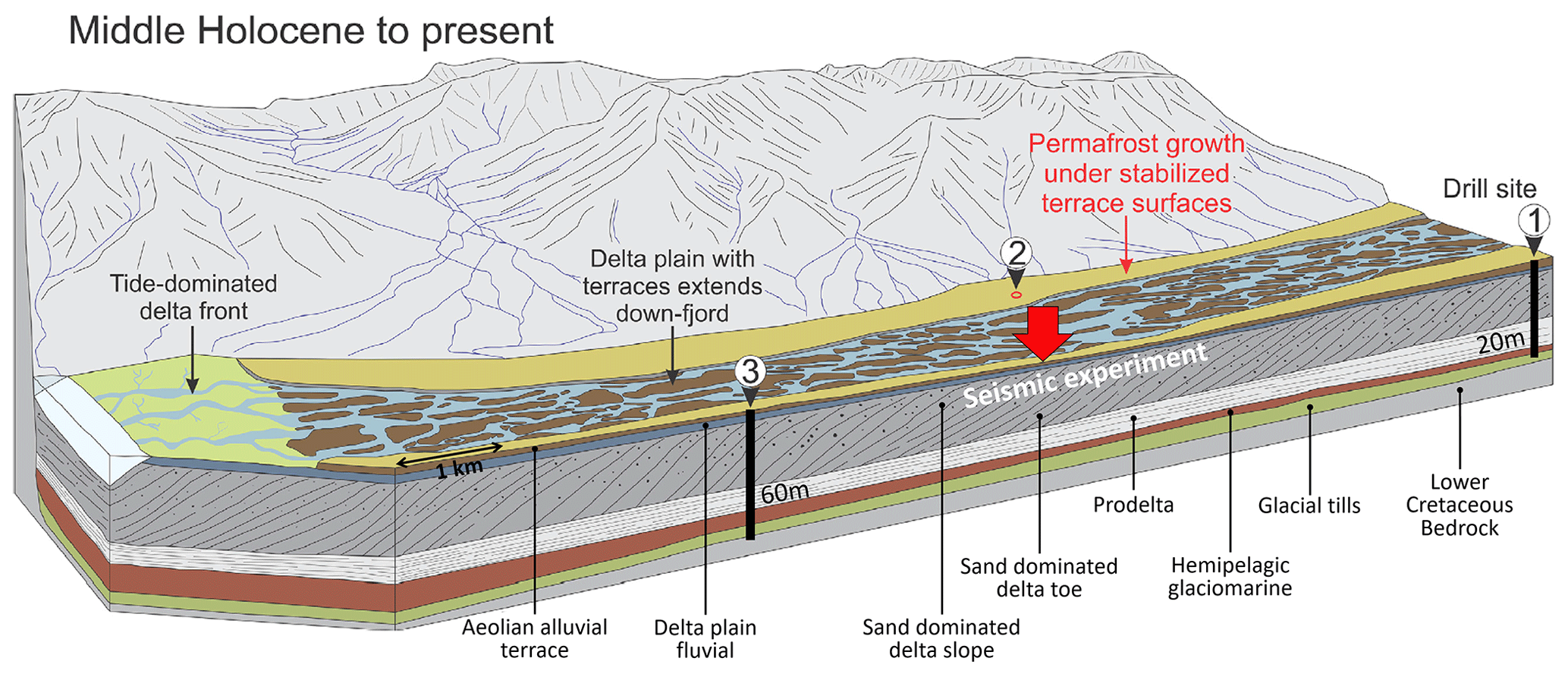
Figure 2Geological model of Adventdalen, Svalbard, modified from Gilbert et al. (2018); the numbered sites mark the coring locations studied by Gilbert et al. (2018), and the red arrow marks the position of the seismic experiments described in this study.
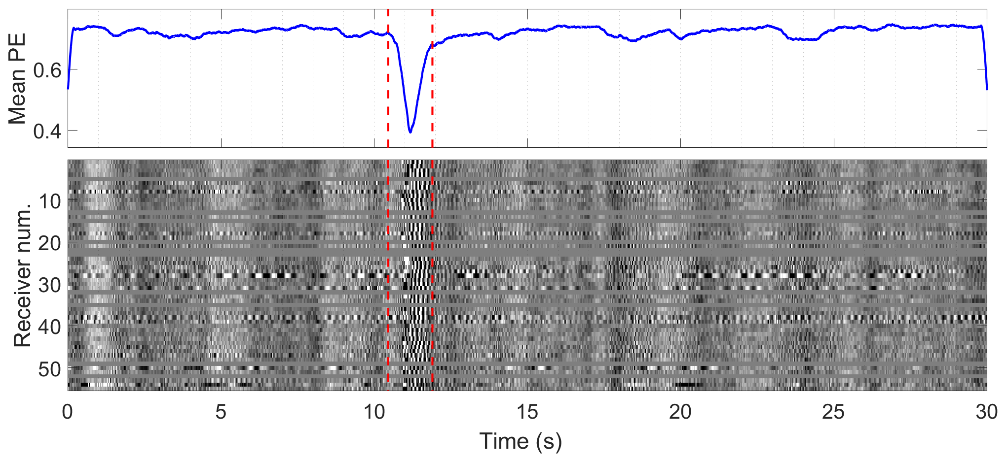
Figure 3Detection of transient event based on mean permutation entropy (PE), a metric that peaks towards minima when coherent amplitudes are recorded across the array of receivers. Red dashed lines mark the temporal extent of the extracted event that is shown in greater detail in Fig. 4. This event was recorded on 30 March 2019 at 18:06 UTC+0.
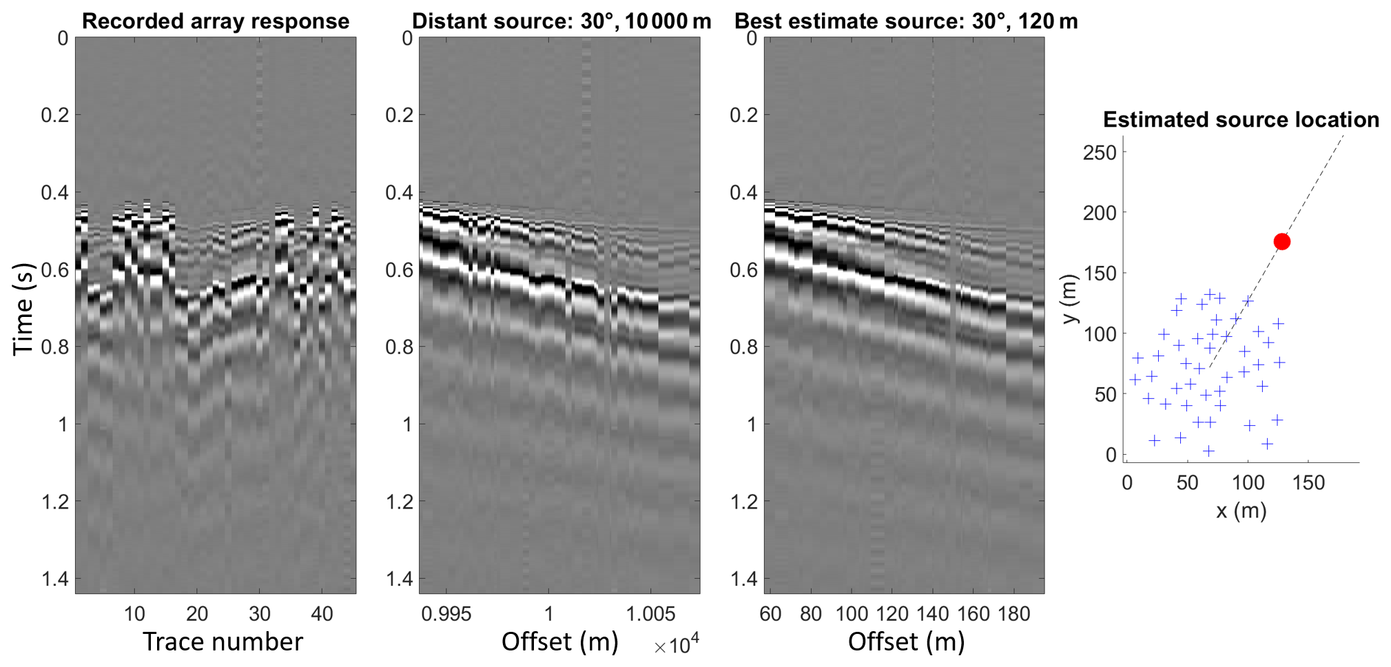
Figure 4Field recording of a transient event, whose detection is highlighted in Fig. 3, demonstrates that re-sorting traces by apparent offset to a distant source produces a gather with poorer coherence than re-sorting by offset to the best-estimate source range at 120 m. Blue crosses denote geophones, while the red circle marks the best-estimate source position.
The isolated microseismic events were subsequently processed in a similar way to active source experiments, i.e. using well-established multichannel analysis of surface waves (MASW) methodologies, with modification due to the unknown source position.
3.2 MASW dispersion imaging with unknown source position
Several processing methods for multichannel analysis of surface waves (MASW) are possible depending on the acquisition setup. One of the most well known is the 1-D phase shift method of Park et al. (1998) that is straightforward to apply for line arrays of receivers and inline sources at known offsets. The dispersion image is built by scanning over frequency (ω) and phase velocity (v) according to
where is the Fourier transform of the ith trace ri(t) of N recorded traces, and is the corresponding phase shift at known source–receiver offset xi. On the other hand, processing of passively recorded microseismic events is complicated by the fact that the source position is unknown. We employed a 2-D receiver array that allows us to localise the unknown passive seismic sources. Again, there are several possibilities to process the 2-D array data. For example, Park et al. (2004) describe an azimuth scanning technique assuming far-field sources and utilising the plane-wave projection principle. The dispersion image is formed according to
where is the Fourier transform of the ith trace , located at position (x,y), of N recorded traces, and and are the phase shifts corresponding to the x and y components of the phase velocity, where θ denotes the source azimuth. We implement this approach by computing, for each combination of velocity and frequency, the azimuth that maximises the spectral magnitude. The source azimuth is thus estimated by calculating the modal azimuth across all frequencies and velocities, and the dispersion spectrum can be formed by fixing the azimuth and reiterating over frequency and velocity axes. The key drawback of forming the dispersion image according to Eq. (2) is that the source must be distant enough that the plane wave assumption is valid. In Fig. 4 we demonstrate that our experimental data are not consistent with the far-field source approximation, since moving the source position closer to the array simplifies the structure of the apparent offset sorted gather. This observation led us to develop an alternative processing approach.
3.3 Two-step MASW approach
We propose a two-step processing approach where the first step involves locating the unknown source position, permitting the dispersion image to be formed in the second step. Even the simplest 1-D phase shift method from Eq. (1) will give superior results to Eq. (2) if a nearby source can be reliably located. Our approach is based on the idea that if the source position was known, the seismic traces from the 2-D array could be arranged by their apparent offset from the source to form a shot gather that resembles the simple case of a line array with an inline source at known offset. Figure 4 shows that when we determine the source azimuth using Eq. (2) and re-sort the recorded traces by offset to a distant source lying along this azimuth we observe that the gather begins to resemble the response of a line array. However, when we shift the assumed source position closer to the array, the offset sorted gather resembles the simple linear array response even more closely. Thus, by formalising a metric that encodes the resemblance of an apparent offset sorted gather to a line array response, we can obtain a useful tool for source localisation that leverages the 2-D array geometry. This further avoids the problem of picking specific P- and S-phase arrivals, a traditional seismological method for source localisation, since these arrivals are difficult to detect reliably in our experimental data.
3.3.1 Step 1 – source localisation
The source is located by re-sorting the seismic traces by offset to a series of test positions. The validity of a given test position is assessed by summing the magnitude of the delays between neighbouring traces in the re-sorted gather. The delays between neighbouring traces are estimated based on the lag that gives maximal value to the normalised cross-correlation between the two signals. The delays are estimated on a relatively narrowband-filtered copy of the seismic (10–15–30–45 Hz Ormsby filter), to minimise the influence of random noise and dispersion. After sorting, the source position is selected as the test position that produces the smallest magnitude sum of adjacent trace delays, corresponding to the simplest and most coherent offset sorted gather. To ensure unphysical velocities are avoided, for each pair of traces we subtract the delay corresponding to a wave travelling the inter-station distance at the maximum expected phase velocity (here we use 2000 m s−1). This simple approach works well in practice and is fast enough to allow a relatively large number of test positions to be evaluated.
In Fig. 5 we show that the source azimuths estimated using this technique are consistent with those estimated by picking maxima in azimuth scans using Eq. (2) but have the additional benefit that the source range is also estimated. Matched-field processing (MFP) is another localisation technique capable of resolving azimuth and range to an unknown source that we include for comparison. We follow the MFP implementation of Walter et al. (2015) but omit the ensemble averaging over multiple seismic noise windows since we are dealing with large-amplitude, distinct microseismic events. Similarly to Walter et al. (2015), we neglect amplitude information and match only the wave phase. The MFP method uses a model of the medium velocity as an additional constraint. We specify the medium velocity as the dominant A0 mode trend picked from the dispersion image formed with Eq. (2). For our catalogue of microseismic events, MFP and our trace re-sorting and delay minimisation method give source locations that we consider equivalent (Fig. 5), since dispersion images corresponding to these source locations were indistinguishable.
The reliability of our source localisation method was further investigated using synthetic gathers corresponding to a set of known source azimuths and ranges. We ran a 1-D noise-free forward model (that accounts for 3-D wave field divergence) using the OASES package for seismo-acoustic propagation in horizontally stratified waveguides, which employs a wave-number-integration solution method (Schmidt and Jensen, 1985). We model the wave field using the layer properties corresponding to the spring field conditions detailed in Table 1. We then specify the receiver positions as deployed in the field and form the synthetic gathers by selecting traces with appropriate offset from the 1-D pre-calculated wave field. The range and azimuth errors produced when attempting to recover the known source positions using the proposed source localisation approach are illustrated in Fig. 6.
The proposed method effectively recovers the direction to the source, regardless of azimuth, although uncertainties relating to the true receiver positions in the field are also important to consider (see Sect. 3.3.3). We also observe reliable estimation of source range within a radius of ∼500 m from the array centre, beyond which we observe an increasing tendency to underestimate the source range (Fig. 6). Further tests with a range of different array geometries indicate that the array aperture is the dominant factor controlling the maximum source range that can be estimated reliably.
3.3.2 Step 2 – dispersion imaging
Once the seismic traces from the 2-D array have been sorted by the apparent offset to the localised source, we are left with a gather that resembles a linear receiver array and an inline source, as seen in Fig. 4. At this point, the dispersion image may simply be formed by applying Eq. (1), i.e. the 1-D phase shift method of Park et al. (1998). However, more advanced processing methodologies have emerged over time, and we observe significantly improved dispersion imaging using the cross-correlation beamforming approach of Le Feuvre et al. (2015), as demonstrated in Fig. 7. This approach utilises the cross-correlations between all possible pairs of receivers, rather than the recorded traces themselves, to increase the effective spatial sampling of the array and thereby reduce aliasing and increase signal-to-noise ratio. In an adaption of this approach, we form the dispersion image, D(ω,v), a function of frequency (ω) and phase velocity (v), according to the following equation using the source position, rs(x,y), estimated as described in Sect. 3.3.1:
with NR the number of receivers and denoting the positions of the receivers for the cross-correlation pair. Furthermore,
Here, the causal cross-correlations and between the receivers located at rj and rk are selected according to the direction of propagation, determined by comparing the two source-to-receiver distances, while the propagation distance is given by the difference between the two. In practice, we do not compute the cross-correlation directly, but instead use the equivalent time-reversed acausal part (negative time delays) of (Le Feuvre et al., 2015). It is important that the seismic traces are pre-whitened prior to computing the cross-correlations, as whitening effectively removes the autocorrelation of the signals that can blur the cross-correlation (El-Gohary and McNames, 2007). We find that a simple first-order backward differencing scheme is an effective method to whiten the recorded traces. We furthermore find it convenient to normalise the frequency response of the dispersion spectrum so that the maximum amplitude along a given frequency is unity.
It should also be noted that it is possible to localise the source by searching for source positions that produce dispersion images with maximum amplitude, as the correct source location is expected to produce the most coherent high-amplitude dispersion modes (Le Feuvre et al., 2015). This approach was tested in the present study. However, we find this method slow and inefficient compared to the trace re-sorting approach we implement, even though maximising dispersion image magnitude does appear to be a valid approach for locating an unknown source.
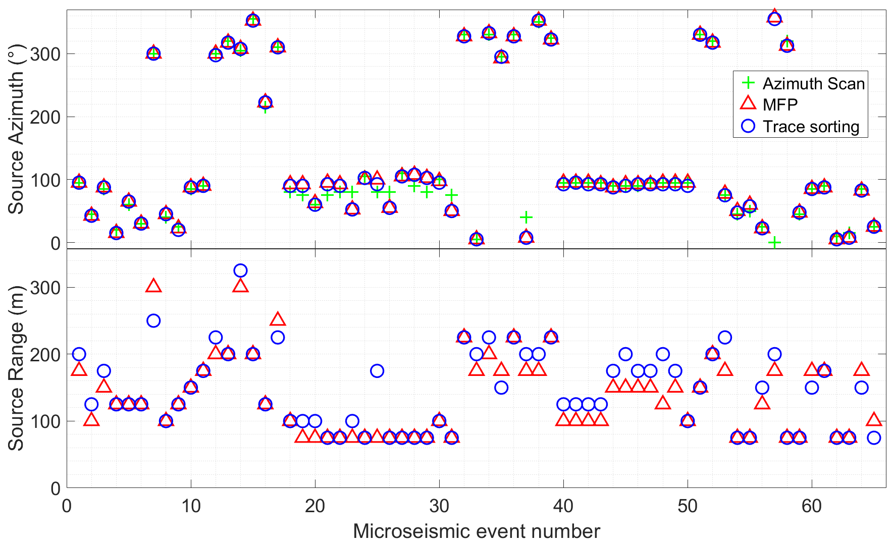
Figure 5Comparison of source localisation using azimuth scanning (i.e. Eq. 2), matched-field processing (MFP), and our trace re-sorting and delay minimisation method. Azimuths are given as compass bearings.
Table 1Physical properties of homogeneous, horizontally layered media used to calculate theoretical dispersion curves shown in Fig. 16. The key feature of the model is a high-velocity surface layer overlying a layer with lower velocity and high Poisson ratio.
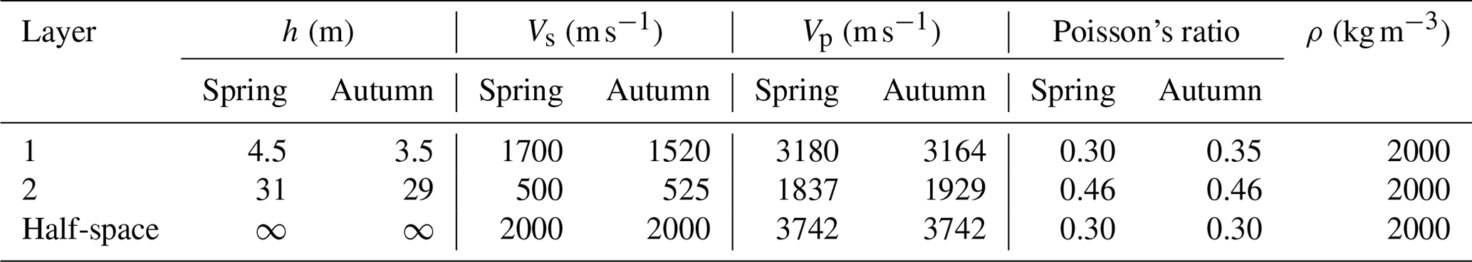

Figure 6Predicted source localisation azimuth and range errors based on forward modelling with known source positions and receiver geometry corresponding to (a) spring and (b) autumn field campaigns.

Figure 7Dispersion spectra with linear colour scaling using the 1-D phase shift method (a) and Le Feuvre et al. (2015) cross-correlation beamforming (b). The microseismic event was recorded on 2 May 2019 at 10:01 UTC+0 at assumed azimuth of 120∘ and range of 140 m.
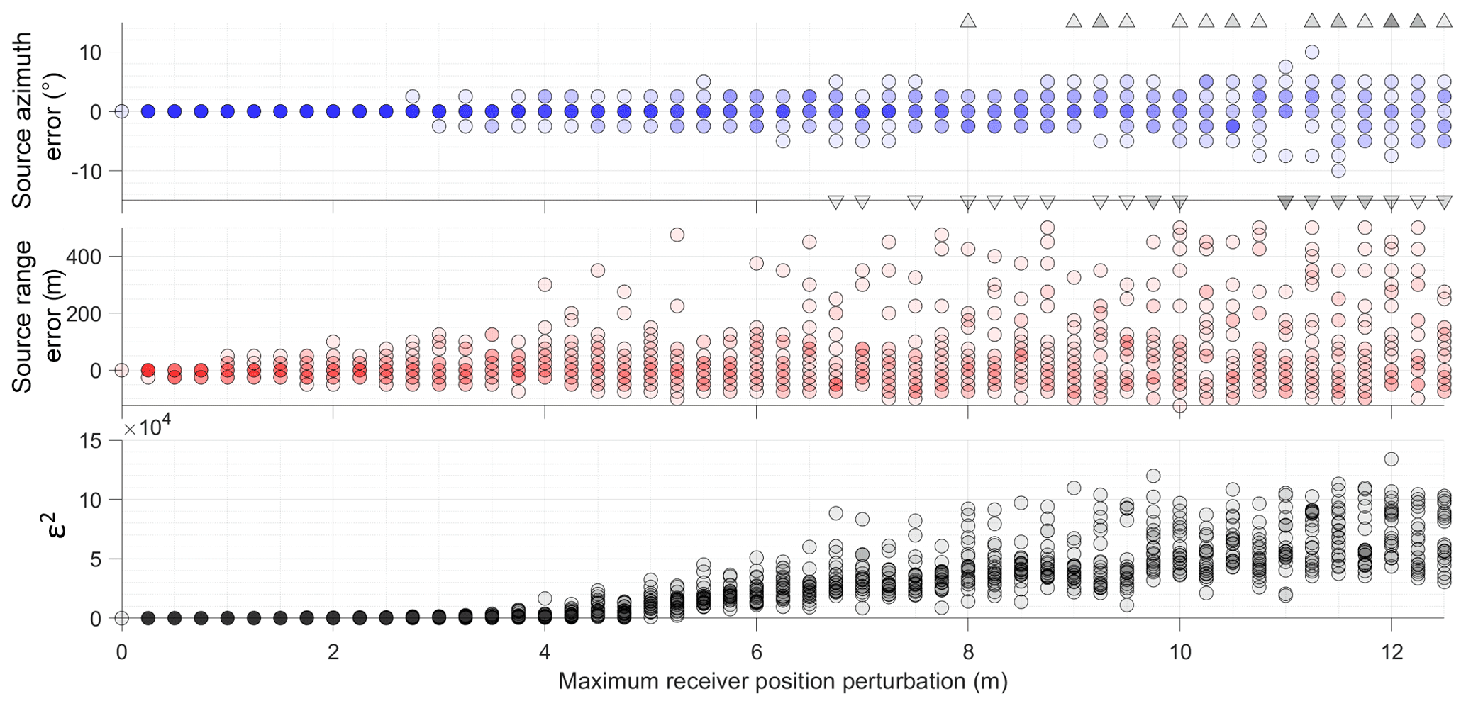
Figure 8Summary of results of 1000 modelling iterations with random white noise perturbation to receiver positions. Grey triangles denote outliers, i.e. iterations that result in large azimuth errors outside the plotted range. Higher colour density denotes overlap, i.e. multiple iterations with the same result. ε2 denotes dispersion spectrum error Eq. (5).
3.3.3 Influence of receiver position errors
During the field campaigns, we recorded GPS positions at the recording nodes that the receivers are connected to rather than at the receivers themselves. The positions of the receivers were subsequently assigned based on approximate dead reckoning and therefore have a degree of uncertainty associated with them. We estimate that this positional uncertainty lies in the range of ∼2–3 m. The impact of receiver position errors was investigated using an OASES 1-D seismo-acoustic propagation model (Schmidt and Jensen, 1985) for the horizontally stratified waveguide corresponding to the spring field conditions detailed in Table 1. We extracted a reference gather assuming a source range of 200 m, azimuth of 100∘ and receiver geometry corresponding to the spring field campaign. We then ran 1000 iterations adding flat-spectrum random perturbations to the receiver positions. In this way we effectively define a circle with a defined radius, where there is equal probability that the receiver is positioned at any given point within this circle. We then measure the impact of these perturbations on both source localisation and dispersion spectra. The dispersion spectrum error (ε2) is given by the sum of squared differences for a given noise-perturbed trial Stest, compared to a noise-free reference spectrum Sref over n frequencies (ω) and m velocities (v):
In Fig. 8 we show that positional errors up to 4–5 m have a very minor impact on source azimuth estimation and dispersion spectra in the frequency range of interest, i.e. up to 100 Hz. Range estimation is somewhat more sensitive (but less important to dispersion spectrum quality), and we see a general trend that the source range tends to be overestimated rather than underestimated. This indicates that the estimated positional uncertainty for the field campaigns (∼2–3 m) should not significantly affect our experimental results, although we may expect some minor overestimation of source range. As the positional error magnitude increases further, Fig. 8 demonstrates that the source localisation becomes progressively more imprecise, while Fig. 9 shows that the maximum frequency imaged coherently in the dispersion spectra progressively decreases. We can formalise this trend by observing the relation that coherent dispersion spectra are recovered for wavelengths of approximately 2–3 times the maximum positional error magnitude.
3.4 Theoretical dispersion curve modelling
The global matrix method was introduced by Knopoff (1964), further elaborated by Lowe (1995) and again by Ryden and Lowe (2004). It involves the assembly of a system matrix S that describes the interaction of displacement and stress fields across interfaces between horizontal layers described by a series of interface matrices. The propagating wave modes are characterised by combinations of frequency (ω) and wave number (k) that satisfy all boundary conditions such that the determinant vanishes:
We abstain from providing a full derivation but give a specific case study that illustrates our implementation and may serve as a simple practical reference point for the reader interested in further exploration of the method. The layer models used in this study contain two discrete layers () bounded by an infinite vacuum half-space above (i=1) and a solid half-space below (i=4), giving the system matrix the following form:
where the matrices describing the top interfaces Dt and the bottom interfaces Db for each layer are given by the following expressions (noting that the minus superscript denotes taking only the upward travelling partial waves given by columns two and four, while the plus superscript denotes selecting only the downward travelling partial waves given by columns one and three):
with
and the physical properties of the system enter as
- hi=
-
thickness of layer i, set to zero for the half-spaces;
- ρi=
-
density of layer i, set to zero for the upper vacuum half-space;
- αi=
-
bulk compressional velocity of layer i, an arbitrary non-zero value for upper vacuum half-space; and
- βi=
-
bulk shear velocity of layer i, an arbitrary non-zero value for upper vacuum half-space.
We are also interested in the magnitude of displacement at the ground surface (top interface of layer i=2) for the different wave modes so that we may predict which are most likely to be excited and subsequently recorded in the field. To this end, we proceed by assuming the amplitudes of the incoming waves in the two half-spaces, setting a unitary amplitude entering the system at the top () and zero amplitude entering the system from below (), allowing us to specify the right-hand side of the following system and solve for the unknown interface amplitudes using a least-squares approach:
Here we substitute the system matrix S for the combinations of frequency and wave number that correspond to the propagating wave modes. The vectors of amplitudes are arranged in the following way:
where L and S denote longitudinal and shear waves respectively, while – and + symbols denote upward and downward travelling partial waves. Having solved for the unknown amplitudes in Eq. (13) we then calculate the displacements and stresses at the ground surface according to the following equation:
where ux and uz denote the complex valued in-plane and vertical displacements, while σzz and σxz denote the complex valued vertical and lateral stresses and the calculation is made at the top interface of layer 2.
In Fig. 10, we show an example of the dispersion curves produced by this approach for the spring layer properties listed in Table 1. Since we measured the vertical component of ground motion in the field, we plot the magnitude of the vertical displacement (uz) as an indicator of the relative likelihood of exciting and subsequently recording specific wave modes. We also highlight, for a given frequency, the wave mode giving the largest displacement at the surface that is considered most likely to dominate the ground response and contribute to the apparent dispersion curve produced by the superposition of multiple modes observed in experimental data.
3.4.1 Numerical root finding method
To recover the dispersion curves it is necessary to find the roots of the system matrix (Eq. 6). In this study, we assume a half-space with higher velocity than the overlying layers, which reflects the presence of compacted sediments and bedrock at depth in Adventdalen. The implication of this choice is that the propagating surface wave modes do not leak energy into the half-space and are much simpler to search for numerically. The permitted surface wave modes are given by combinations of frequency and phase velocity (or wave number) that minimise the determinant of the system matrix. We localise these minima by conducting a simple 2-D numerical search over a regular grid of frequency and real wave number (the imaginary part of the wave number is zeroed since we consider only non-leaky modes). The local minima in the matrix sampling the determinant of the system matrix are found by morphological image processing techniques rather than the more traditional method of curve tracing using bisection algorithms favoured by for example Lowe (1995). Specifically, we use the imregionalmax routine in MATLAB on the negative of the determinant matrix, applying a series of linear connectivity kernels for detection of local maxima ridges. We then mask out non-dispersive body waves that appear as horizontal ridges in frequency-phase velocity space and use morphological closing operations to fill in the gaps that this creates. We further apply skeletonisation to the binary image of dispersion curves. The non-zero elements of the binary matrix then define the combinations of frequency and velocity that represent the dispersive wave modes and that are subsequently used to calculate surface wave amplitudes with Eq. (13).
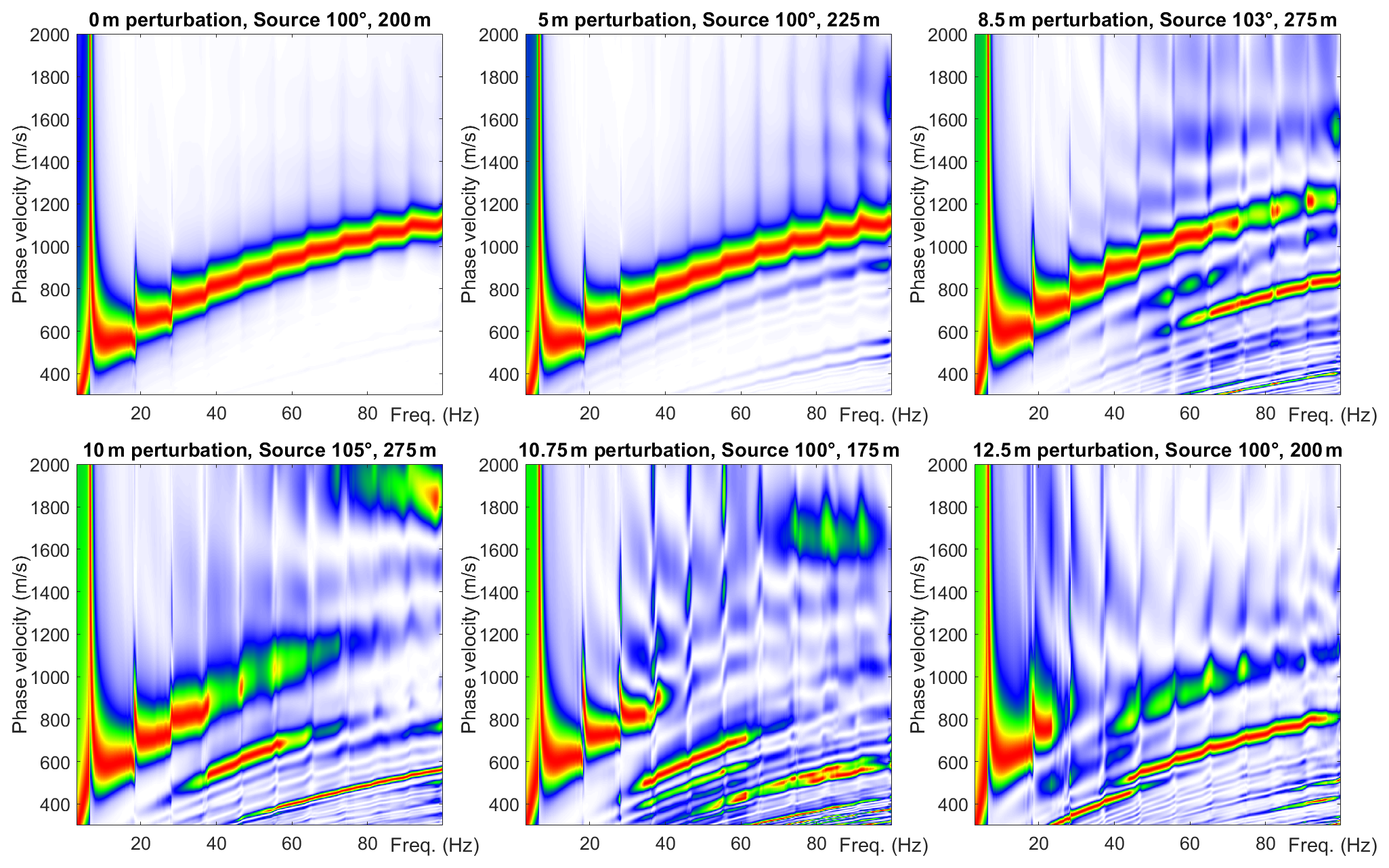
Figure 9Dispersion spectra calculated from forward model with receiver positions perturbed by white random noise of indicated magnitude illustrating how the maximum frequency that is coherently imaged decreases with increasing uncertainty in receiver position. The true source position is at 100∘, range 200 m. Colour scale is linear.
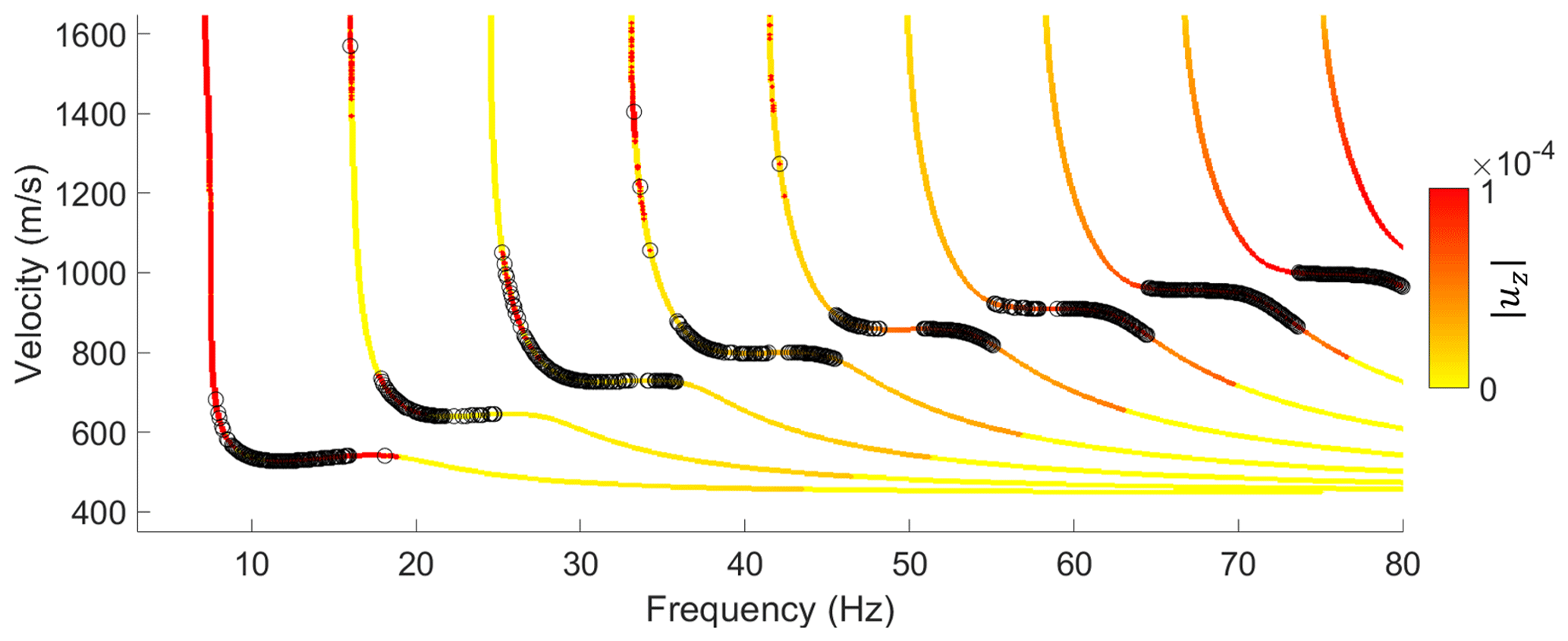
Figure 10Example of theoretical dispersion curves coloured by magnitude of vertical displacement at the ground surface. Black circles denote the wave mode with largest displacement for a particular frequency.
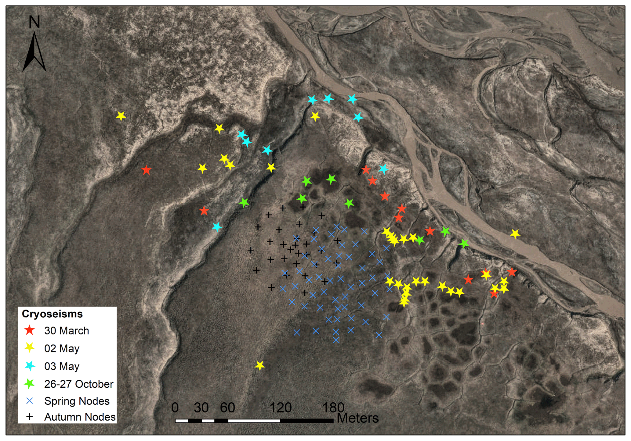
Figure 11Localised source positions (coloured stars) and receiver positions for spring (cross symbols) and autumn (plus symbols) field campaigns; background is a contrast-enhanced version of an orthophoto © Norwegian Polar Institute (http://npolar.no).
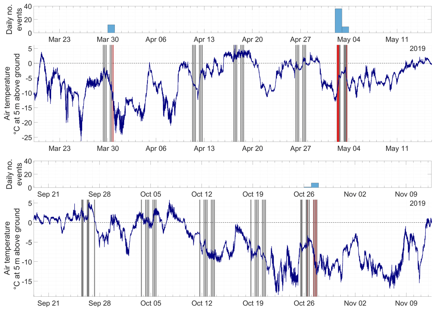
Figure 12Temperature at 5 m above ground at nearby weather station in Adventdalen. Grey bars denote periods when passive seismic data were recorded, and red bars denote periods where transient seismic events producing multimodal dispersion spectra were detected.
4.1 Interpretation of cryoseisms
A series of transient seismic events were isolated from passive seismic recordings of 2-D geophone arrays deployed at our study site in Adventdalen. The estimated source positions for these events are shown in Fig. 11, while their temporal occurrence is illustrated in Fig. 12. The events cluster primarily around frost polygons along the raised river terrace. A small number of events fall just beyond the raised riverbank and plot within the Adventelva river valley. While these events may be correctly located, we also cannot rule out the possibility that they occurred on the raised terrace and the source range has been overestimated as discussed in Sect. 3.3.3. Figure 12 shows that the transient events were all recorded during periods of rapidly changing air temperature as recorded at a nearby weather station. This observation together with the spatial clustering around frost polygons and on the raised river terrace, which is known to have high ground-ice content within the upper ∼4 m (Gilbert et al., 2018), leads us to infer that these events are most likely cryoseisms, or frost quakes. The fact that these events consist dominantly of surface wave energy is also consistent with a shallow source and previous descriptions of cryoseisms (Barosh, 2000). Similarly, the fact that the source range for all of the recorded events was in the order of hundreds of metres is also consistent with the distance over which previously observed cryoseisms have propagated (Leung et al., 2017; Nikonov, 2010), and we are unaware of any other likely seismic sources within this range. Other possible seismic sources include an operational coal mine, Gruve 7, that conducts blasting operations ∼5 km to the SE. Road traffic ∼650–850 m S–SW and snowmobile traffic along the Adventelva river valley N–E of the study site are also possible sources. However, these sources do not explain the spatial distribution and character of the recorded events. Known examples of snowmobile and vehicle traffic contain strong air wave arrivals with non-dispersive velocity of ∼320–330 m s−1 that was not observed for the class of events attributed to cryoseisms.
The temporal resolution of this study is limited due to the fact that data were recorded during specific intervals rather than continuously (see Fig. 12). This means that additional cryoseisms may have occurred under rapid cooling events during the field campaigns for which no data were recorded. However, we can observe that the recording windows for which no cryoseisms were detected were associated with temperatures that were either too high or changing slowly in comparison to the periods when cryoseisms were detected. The frequency of cryoseisms was greater during the spring compared to the autumn, probably owing to the increased progression of ground freezing in the aftermath of cold winter air temperatures. It is interesting to note that the highest frequency of cryoseisms was recorded on 2 May 2019 during a period when the air temperature was rapidly increasing and following a sharp cold snap down from above-freezing temperatures 3 d prior. It is unclear whether these events are a delayed effect of the preceding cold snap, where the subsurface stress continues to increase for some time after the drop in air temperature, or if the events are caused by the sharp temperature rise itself and associated with cracking driven by thermal expansion rather than contraction. We also note that snow cover on the raised river terrace was thin or absent during the field campaigns, due to relatively low precipitation and strong prevailing winds. The lack of an insulating snow layer increases the plausibility of correlating air temperature at 5 m above ground with cryoseismic events in the shallow subsurface and has been recognised as a necessary condition facilitating sufficiently rapid ground cooling to generate cryoseisms in previous studies (Barosh, 2000; Battaglia and Chagnon, 2016; Matsuoka et al., 2018; Nikonov, 2010).
4.2 Dispersion images and temporal variation
Dispersion images from the isolated cryoseisms resemble the complex multimodal dispersion of Lamb–Rayleigh waves that is relatively well known from pavement studies (Ryden and Lowe, 2004; Ryden et al., 2004). This complexity emerges when a stiff high-velocity layer overlies a softer layer producing an inversion in the shear velocity profile and acting as a waveguide. Some examples of estimated dispersion spectra are shown in Fig. 13 spanning both spring and autumn field campaigns. We observe that the number of wave-mode branches imaged in the spring records was higher than in the autumn over the investigated range of frequencies. In Fig. 14, we compare individual events from spring and autumn, and we observe that the apparent dispersion curve is shifted towards lower velocities in the autumn and that transitions between successive modes are shifted to higher frequencies with larger spacing between modes. This trend is robust across the catalogue of cryoseisms giving well-resolved dispersion images, as shown in Fig. 15, displaying the time-frequency-traced ridges of dispersion images corresponding to multiple records from spring and autumn field campaigns. MATLAB's built-in routine tfridge was found to be effective for ridge tracing in this study.
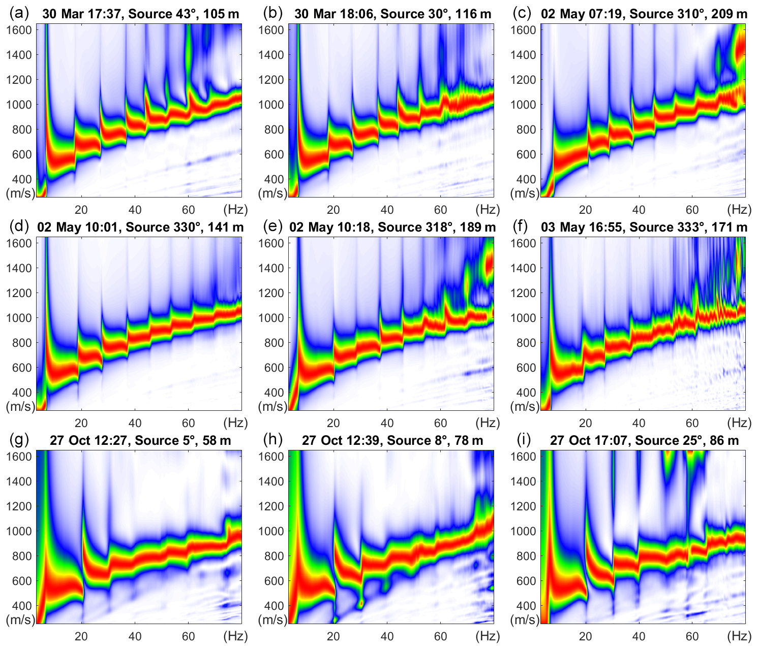
Figure 13Examples of dispersion spectra for selected cryoseismic events from spring (a–f) and autumn (g–i) field campaigns; source azimuths are given as compass bearings and colour scaling is linear.
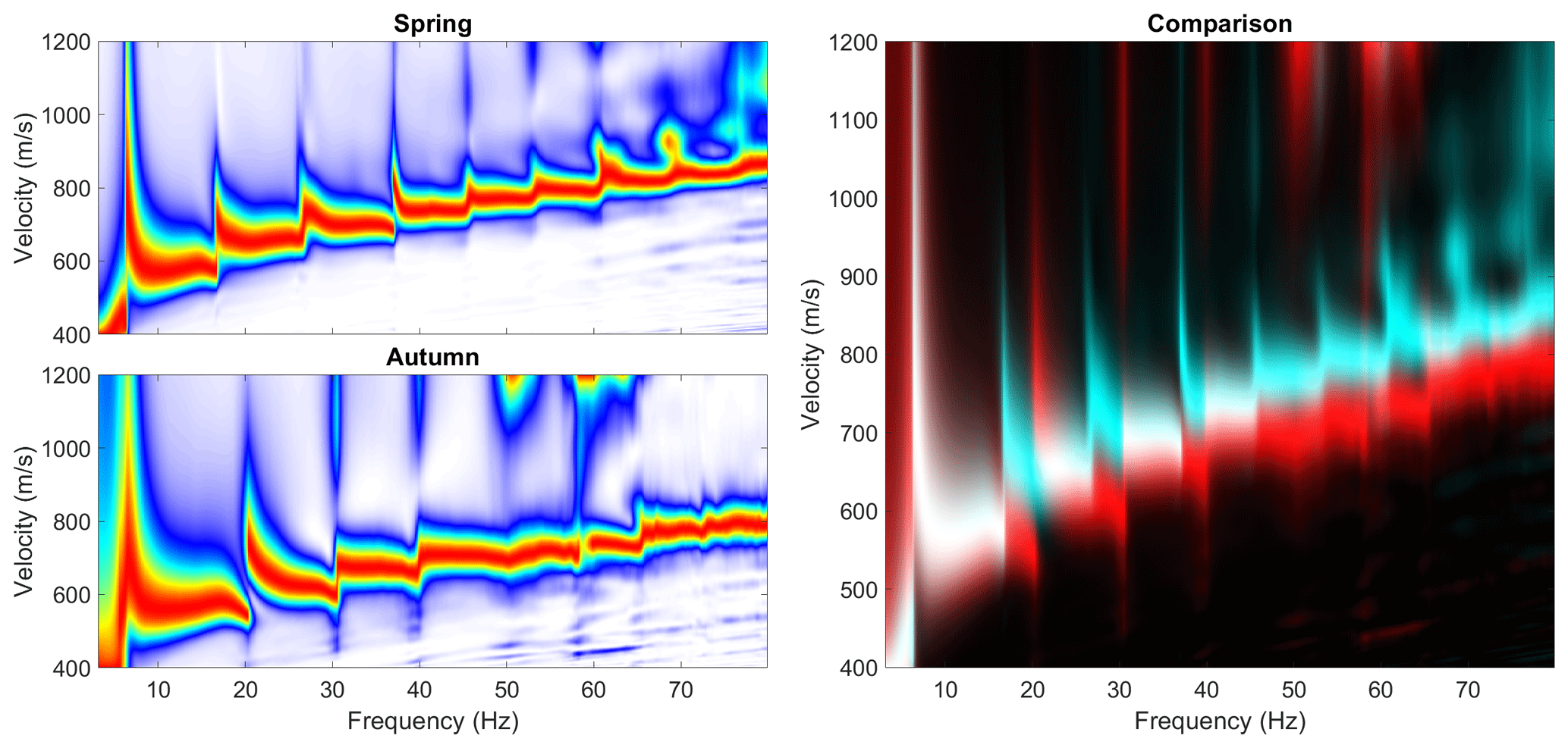
Figure 14Comparison of records from spring and autumn; in the right panel the spring record is shown in cyan and the autumn record is shown in red, and areas where the two spectra overlap appear white.
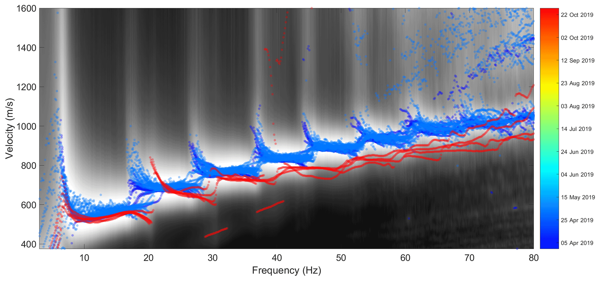
Figure 15Illustration of temporal variation. Greyscale background image shows the mean dispersion spectrum for all displayed transient events. Coloured circles denote time frequency ridges picked from individual dispersion spectra and coloured according to date of recording.
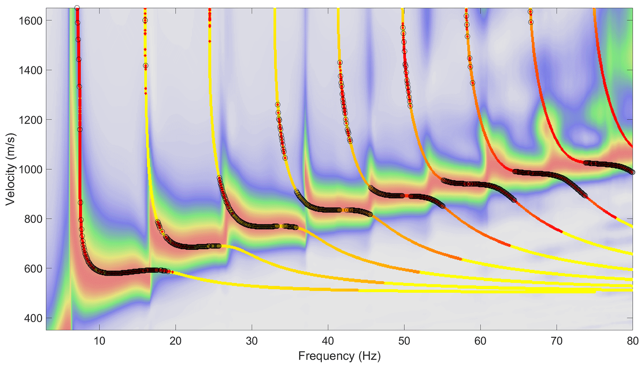
Figure 16Spring field campaign best-qualitative-fit theoretical dispersion curves, based on a simple three-layer horizontal model (see Table 1). Dispersion spectrum corresponds to event recorded on 2 May at 06:51 UTC+0, displayed with linear colour scaling.
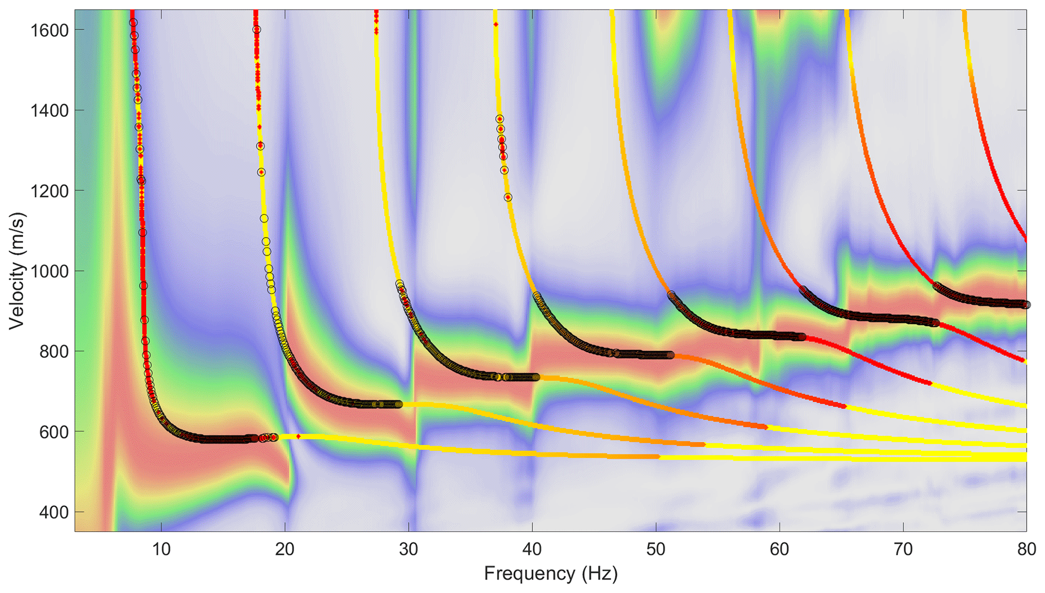
Figure 17Autumn field campaign best-qualitative-fit theoretical dispersion curves, based on a simple three-layer horizontal model (see Table 1). Dispersion spectrum corresponds to event recorded on 27 October at 12:27 UTC+0, displayed with linear colour scaling.
In addition to temporal variation in ground structure, one might anticipate that the varying receiver footprint or lateral variation in ground structure could also contribute to the observed variation in dispersion spectra. Based on dispersion imaging of synthetic test data, we are confident that the varying receiver footprint does not play a significant role for a laterally homogenous, horizontally layered medium. Further, we observe that dispersion images for spatially dispersed events over short time windows (24–48 h) are highly consistent, which points towards a ground structure that is relatively consistent laterally. On the other hand, events that cluster spatially while being dispersed temporally show significant variation. The dominant trend is well illustrated in Fig. 15, i.e. events within a given season are quite similar despite variation in source location, but there is significant variation between events occurring at different times of the year. These observations are consistent with the interpretation that the variation in surface wave dispersion is mainly caused by temporal variation in ground structure.
4.3 Inferring subsurface structure from dispersion images
To further investigate what the structure of the dispersion images tells us about the subsurface permafrost structure and its variation between spring and autumn field campaigns, we ran a series of theoretical models using the global matrix approach discussed in Sect. 3.4. These models were optimised manually by qualitatively fitting the resulting dispersion curves with experimental dispersion images and manually adjusting the physical parameters to achieve a best possible fit. We focussed our attention on the simplest possible models that give a good approximation of the experimental data, which in this case meant two discrete layers with an inverse velocity profile sandwiched between infinite vacuum (above) and solid (below) half-spaces. The physical properties of the best-estimate models corresponding to spring and autumn conditions are listed in Table 1.
The primary property of the models that allows us to fit the experimental data is the high velocity of the uppermost part of the ground, overlying relatively low velocity material beneath. We also see evidence that the Poisson ratio in the low-velocity layer is relatively high (0.46), consistent with a softer material that transmits shear stress less effectively. The physical manifestation of the high-velocity surface layer is likely to be the zone of elevated ground-ice content of ∼4 m thickness observed in the Adventdalen boreholes of Gilbert et al. (2018). This zone is rich in void-filling ice, lenticular and massive solid bodies of ice that macroscopically strengthen the dominantly loess sediments (Gilbert et al., 2018), leading to relatively high shear wave velocity and a relatively low Poisson ratio.
The low-velocity layer may simply reflect the absence of these stiffening ice bodies and subsequently decreased shear strength in the porous medium. However, the low-velocity zone may also indicate the presence of unfrozen permafrost due to elevated salinity, recalling that permafrost is defined simply as ground that remains below 0 ∘C over at least 2 consecutive years, but does not imply that the ground is in fact frozen. This interpretation is supported by the high Poisson ratio of the lower layer, since according to Skvortsov et al. (2014) a Poisson ratio of 0.45–0.46 represents a threshold between frozen and unfrozen states for water-saturated soils, irrespective of composition, temperature and salinity. Furthermore, nuclear magnetic resonance and controlled source audio-magnetotelluric data suggest the presence of unfrozen saline permafrost below the Holocene marine limit in Adventdalen (Keating et al., 2018). On balance, we conclude that unfrozen saline permafrost is the most likely explanation for the observed low-velocity zone.
In Fig. 16 we see that the theoretical dispersion curves fit the experimental data recorded in spring remarkably well, given our simplistic layer model. Figure 17 illustrates that the fit between model and experimental data is somewhat poorer for the autumn, although good overall fit was still achieved. Reasons for this contrast may include that the cryoseisms were stronger in spring due to colder temperatures and a more advanced state of freezing, leading to a more broadband source signal. Alternately, the ground may have been more heterogeneous in the autumn, as indicated by interspersed ponds of unfrozen water and ice observed at the study site when deploying geophones in September compared with a relatively homogeneous frozen landscape with thin snow cover in March. This increased heterogeneity may affect the experimentally recorded events either via attenuation of the surface waves between source and receiver or by heterogeneities across the geophone array itself, leading to decreased coherency.
It was difficult to fit the steep phase velocity gradients at the frequencies where the ground response transitions from one wave mode to another using our simplistic layer model (particularly noticeable for modes 3–6 in Fig. 16). We have not investigated this phenomenon in detail but hypothesise that some additional degree of freedom such as allowing for velocity gradients within layers may be required to improve this aspect of the fit. In general, it would be advantageous to develop an inversion scheme capable of robustly selecting the physical model(s) that best fits the observed dispersion spectra. However, we anticipate that this would be a complex task due to the non-uniqueness and non-linearity of the problem, exacerbated by the complex multimodal dispersion structure. These factors make it difficult to optimise inversion parameters by exploiting partial derivatives. While developing a suitable inversion scheme fell outside the scope of this study, we direct the interested reader towards the study of Ryden and Park (2006). They implemented a global optimisation approach based on the fast-simulated annealing algorithm to invert multimodal surface waves recorded in pavement. Their scheme appears capable of dealing with the problems of cost-function local minima and correlated parameters, assuming that the parameter perturbation size and cooling schedule of the simulated annealing can be adequately tuned for the specific set of dispersion spectra.
We present a methodology designed to isolate transient seismic events in passive records and thereby estimate their unknown source location and image their phase velocity dispersion. The spatial association of the source positions with a well-known frost polygon area along an elevated river terrace in Adventdalen, together with temporal correlation with periods of rapidly changing air temperature, indicates that these events are likely cryoseisms. The phase velocity dispersion of these cryoseisms furthermore allows us to infer the subsurface structure of the permafrost and detect changes between seasons. A high-velocity solid-frozen surface layer overlying a slower and softer layer leads to a complex multimodal dispersion pattern that is familiar from previous studies of pavements. The uppermost part of the permafrost appears to be measurably softer during the autumn than the spring, implying that this methodology may also have the potential to detect changes in an inter-annual monitoring context. A future field campaign recording continuously over an entire freeze season would, for example, give a more complete picture of the spatio-temporal occurrence of cryoseisms. Alternatively, our methodology could be applied for other locations with suitable seismic sources, such as on or adjacent to glaciers.
Data and code used to produce this research can be shared upon request to the authors.
The field campaigns were administered by TAJ and carried out by RR, BOR, HMS and TAJ. Initial data collation and processing was carried out by BOR. Exploratory data analysis was conducted by RR and HMS. The data processing methodology was developed and implemented by RR in collaboration with AH. Finite difference modelling was carried out by BOR and dispersion curve models by RR and AH. RR was responsible for analysing and visualising the data and writing the manuscript with contributions from all authors.
The authors declare that they have no conflict of interest.
This research has been supported by the University of Tromsø – The Arctic University of Norway, ARCEx partners and the Research Council of Norway (grant no. 228107).
This paper was edited by Adam Booth and reviewed by Aurélien Mordret and one anonymous referee.
Bandt, C. and Pompe, B.: Permutation entropy: a natural complexity measure for time series, Phys. Rev. Lett., 88, 174102, https://doi.org/10.1103/PhysRevLett.88.174102, 2002.
Barosh, P. J.: Frostquakes in New England, Eng. Geol., 56, 389–394, 2000.
Battaglia, S. M. and Changnon, D.: Frost Quakes: Forecasting the Unanticipated Clatter, Weatherwise, 69, 20–27, https://doi.org/10.1080/00431672.2015.1109984, 2016.
Cable, S., Elberling, B., and Kroon, A.: Holocene permafrost history and cryostratigraphy in the High Arctic Adventdalen Valley, central Svalbard, Boreas, 47, 423–442, 2018.
Chillara, V. K. and Lissenden, C. J.: Review of nonlinear ultrasonic guided wave nondestructive evaluation: theory, numerics, and experiments, Opt. Eng., 55, 011002, https://doi.org/10.1117/1.OE.55.1.011002, 2015.
Christiansen, H. H., Etzelmüller, B., Isaksen, K., Juliussen, H., Farbrot, H., Humlum, O., Johansson, M., Ingeman-Nielsen, T., Kristensen, L., and Hjort, J.: The thermal state of permafrost in the Nordic area during the International Polar Year 2007–2009, Permafrost Periglac., 21, 156–181, 2010.
Christiansen, H. H., Matsuoka, N., and Watanabe, T.: Progress in understanding the dynamics, internal structure and palaeoenvironmental potential of ice wedges and sand wedges, Permafrost Periglac., 27, 365–376, 2016.
Dou, S., Nakagawa, S., Dreger, D., and Ajo-Franklin, J.: An effective-medium model for P-wave velocities of saturated, unconsolidated saline permafrost, Geophysics, 82, EN33–EN50, 2017.
El-Gohary, M. and McNames, J.: Establishing causality with whitened cross-correlation analysis, IEEE T. Bio.-Med.-Eng., 54, 2214–2222, 2007.
Foti, S., Hollender, F., Garofalo, F., Albarello, D., Asten, M., Bard, P.-Y., Comina, C., Cornou, C., Cox, B., and Di Giulio, G.: Guidelines for the good practice of surface wave analysis: A product of the InterPACIFIC project, B. Earthq. Eng., 16, 2367–2420, 2018.
French, H. M.: The periglacial environment, 4th edn., John Wiley and Sons, Hoboken, New Jersey, USA, 2017.
Gilbert, G. L., Kanevskiy, M., and Murton, J. B.: Recent advances (2008–2015) in the study of ground ice and cryostratigraphy, Permafrost Periglac., 27, 377–389, 2016.
Gilbert, G. L., O'neill, H. B., Nemec, W., Thiel, C., Christiansen, H. H., and Buylaert, J. P.: Late Quaternary sedimentation and permafrost development in a Svalbard fjord-valley, Norwegian high Arctic, Sedimentology, 65, 2531–2558, 2018.
Humlum, O., Instanes, A., and Sollid, J. L.: Permafrost in Svalbard: a review of research history, climatic background and engineering challenges, Polar Res., 22, 191–215, 2003.
Johansen, T. A., Digranes, P., van Schaack, M., and Lønne, I.: Seismic mapping and modeling of near-surface sediments in polar areas, Geophysics, 68, 566–573, 2003.
Kanevskiy, M., Shur, Y., Fortier, D., Jorgenson, M., and Stephani, E.: Cryostratigraphy of late Pleistocene syngenetic permafrost (yedoma) in northern Alaska, Itkillik River exposure, Quaternary Res., 75, 584–596, 2011.
Keating, K., Binley, A., Bense, V., Van Dam, R. L., and Christiansen, H. H.: Combined geophysical measurements provide evidence for unfrozen water in permafrost in the adventdalen valley in Svalbard, Geophys. Res. Lett., 45, 7606–7614, 2018.
Knopoff, L.: A matrix method for elastic wave problems, B. Seismol. Soc. Am., 54, 431–438, 1964.
Kottek, M., Grieser, J., Beck, C., Rudolf, B., and Rubel, F.: World map of the Köppen-Geiger climate classification updated, Meteorol. Z., 15, 259–263, 2006.
Lachenbruch, A. H.: Mechanics of thermal contraction cracks and ice-wedge polygons in permafrost, Geol. Soc. Am., The Waverly Press, Baltimore, Maryland, USA, 1962.
Le Feuvre, M., Joubert, A., Leparoux, D., and Cote, P.: Passive multi-channel analysis of surface waves with cross-correlations and beamforming. Application to a sea dike, J. Appl. Geophys., 114, 36–51, 2015.
Leung, A. C., Gough, W. A., and Shi, Y.: Identifying frostquakes in Central Canada and neighbouring regions in the United States with social media, in: Citizen Empowered Mapping, Springer, Cham, Switzerland, 2017.
Lønne, I.: Faint traces of high Arctic glaciations: an early Holocene ice-front fluctuation in Bolterdalen, Svalbard, Boreas, 34, 308–323, 2005.
Lowe, M. J.: Matrix techniques for modeling ultrasonic waves in multilayered media, IEEE T. Ultrason. Ferr., 42, 525–542, 1995.
Mackay, J. R.: The direction of ice-wedge cracking in permafrost: downward or upward?, Can. J. Earth Sci., 21, 516–524, 1984.
Matsuoka, N., Christiansen, H. H., and Watanabe, T.: Ice-wedge polygon dynamics in Svalbard: Lessons from a decade of automated multi-sensor monitoring, Permafrost Periglac., 29, 210–227, 2018.
Nikonov, A.: Frost quakes as a particular class of seismic events: Observations within the East-European platform, Izvestiya, Phys. Solid Earth, 46, 257–273, 2010.
O'Neill, H. B. and Christiansen, H. H.: Detection of ice wedge cracking in permafrost using miniature accelerometers, J. Geophys. Res.-Earth, 123, 642–657, 2018.
O'Neill, H. B. and Burn, C. R.: Physical and temporal factors controlling the development of near-surface ground ice at Illisarvik, western Arctic coast, Canada, Can. J. Earth Sci., 49, 1096–1110, 2012.
Park, C., Miller, R., Laflen, D., Neb, C., Ivanov, J., Bennett, B., and Huggins, R.: Imaging dispersion curves of passive surface waves, in: SEG technical program expanded abstracts 2004, Society of Exploration Geophysicists, Tulsa, Oklahoma, USA, 1357–1360, https://doi.org/10.1190/1.1851112, 2004.
Park, C. B., Miller, R. D., and Xia, J.: Imaging dispersion curves of surface waves on multi-channel record, in: SEG Technical Program Expanded Abstracts 1998, Society of Exploration Geophysicists, Tulsa, Oklahoma, USA, 1377–1380, https://doi.org/10.1190/1.1820161, 1998.
Park, C. B., Miller, R. D., and Xia, J.: Multichannel analysis of surface waves, Geophysics, 64, 800–808, 1999.
Park, C. B., Miller, R. D., Xia, J., and Ivanov, J.: Multichannel analysis of surface waves (MASW) – active and passive methods, Leading Edge, 26, 60–64, 2007.
Rose, J. L.: Ultrasonic Guided Waves in Structural Health Monitoring, Key Engineering Materials, 11th Asian Pacific Conference on Nondestructive Testing (llth-APCNDT), Jeju island, Korea, 3–7 November 2003, Trans Tech Publications, Ltd., 270–273, 14–21, https://doi.org/10.4028/www.scientific.net/kem.270-273.14, 2004.
Ryden, N. and Lowe, M. J.: Guided wave propagation in three-layer pavement structures, J. Acoust. Soc. Am., 116, 2902–2913, 2004.
Ryden, N. and Park, C. B.: Fast simulated annealing inversion of surface waves on pavement using phase-velocity spectra, Geophysics, 71, R49–R58, 2006.
Ryden, N., Park, C. B., Ulriksen, P., and Miller, R. D.: Multimodal approach to seismic pavement testing, J. Geotech. Geoenviron., 130, 636–645, 2004.
Schmidt, H. and Jensen, F. B.: A full wave solution for propagation in multilayered viscoelastic media with application to Gaussian beam reflection at fluid–solid interfaces, J. Acoust. Soc. Am., 77, 813–825, 1985.
Sergeant, A., Chmiel, M., Lindner, F., Walter, F., Roux, P., Chaput, J., Gimbert, F., and Mordret, A.: On the Green's function emergence from interferometry of seismic wave fields generated in high-melt glaciers: implications for passive imaging and monitoring, The Cryosphere, 14, 1139–1171, https://doi.org/10.5194/tc-14-1139-2020, 2020.
Skvortsov, A., Sadurtdinov, M., and Tsarev, A.: Seismic Criteria for Identifying Frozen Soil, Kriosfera Zemli, 18, 75–80, 2014.
Unakafova, V. and Keller, K.: Efficiently measuring complexity on the basis of real-world data, Entropy, 15, 4392–4415, 2013.
Walter, F., Roux, P., Roeoesli, C., Lecointre, A., Kilb, D., and Roux, P.-F.: Using glacier seismicity for phase velocity measurements and Green's function retrieval, Geophys. J. Int., 201, 1722–1737, 2015.