the Creative Commons Attribution 4.0 License.
the Creative Commons Attribution 4.0 License.
 | 18 Jun 2021
The retrieval of snow properties from SLSTR Sentinel-3 – Part 2: Results and validation
Linlu Mei
Vladimir Rozanov
Evelyn Jäkel
Xiao Cheng
Marco Vountas
John P. Burrows
To evaluate the performance of the eXtensible Bremen Aerosol/cloud and surfacE parameters Retrieval (XBAER) algorithm, presented in the Part 1 companion paper to this paper, we apply the XBAER algorithm to the Sea and Land Surface Temperature Radiometer (SLSTR) instrument on board Sentinel-3. Snow properties – snow grain size (SGS), snow particle shape (SPS) and specific surface area (SSA) – are derived under cloud-free conditions. XBAER-derived snow properties are compared to other existing satellite products and validated by ground-based and aircraft measurements. The atmospheric correction is performed on SLSTR for cloud-free scenarios using Modern-Era Retrospective Analysis for Research and Applications (MERRA) aerosol optical thickness (AOT) and the aerosol typing strategy according to the standard XBAER algorithm. The optimal SGS and SPS are estimated iteratively utilizing a look-up-table (LUT) approach, minimizing the difference between SLSTR-observed and SCIATRAN-simulated surface directional reflectances at 0.55 and 1.6 µm. The SSA is derived for a retrieved SGS and SPS pair. XBAER-derived SGS, SPS and SSA have been validated using in situ measurements from the recent campaign SnowEx17 during February 2017. The comparison shows a relative difference between the XBAER-derived SGS and SnowEx17-measured SGS of less than 4 %. The difference between the XBAER-derived SSA and SnowEx17-measured SSA is 2.7 m2/kg. XBAER-derived SPS can be reasonably explained by the SnowEx17-observed snow particle shapes. Intensive validation shows that (1) for SGS and SSA, XBAER-derived results show high correlation with field-based measurements, with correlation coefficients higher than 0.85. The root mean square errors (RMSEs) of SGS and SSA are around 12 µm and 6 m2/kg. (2) For SPS, aggregate SPS retrieved by XBAER algorithm is likely to be matched with rounded grains while single SPS in XBAER is possibly linked to faceted crystals.
The comparison with aircraft measurements, during the Polar Airborne Measurements and Arctic Regional Climate Model Simulation Project (PAMARCMiP) campaign held in March 2018, also shows good agreement (with R=0.82 and R=0.81 for SGS and SSA, respectively). XBAER-derived SGS and SSA reveal the variability in the aircraft track of the PAMARCMiP campaign. The comparison between XBAER-derived SGS results and the Moderate Resolution Imaging Spectroradiometer (MODIS) Snow-Covered Area and Grain size (MODSCAG) product over Greenland shows similar spatial distributions. The geographic distribution of XBAER-derived SPS over Greenland and the whole Arctic can be reasonably explained by campaign-based and laboratory investigations, indicating a reasonable retrieval accuracy of the retrieved SPS. The geographic variabilities in XBAER-derived SGS and SSA both over Greenland and Arctic-wide agree with the snow metamorphism process.
- Article
(12317 KB) - Full-text XML
- Companion paper
- BibTeX
- EndNote


Change in snow properties is both a consequence and a driver of climate change (Barnett et al., 2005). Snow cover and snow season, especially in the Northern Hemisphere, are reported by different models to decrease due to climate change (Liston and Hiemstra, 2011). The reduction in snow cover leads to a change in the surface energy budget (Cohen and Rind, 1991; Henderson et al., 2018), a reduction in Asian summer rainfall (Liu and Yanai, 2002; Zhang et al., 2019), a loss of Arctic plant species (Phoenix, 2018), and other impacts on societies and ecosystems (Bokhorst et al., 2016). Snow may influence the climate through both direct and indirect feedbacks (Lemke et al., 2007). The direct feedback is the snow–albedo feedback, and the indirect feedbacks involve atmospheric circulation. The snow–albedo feedback describes the mechanism by which melting snow (the absence of snow cover), caused by global warming, reflects less solar radiation and further enhances the warming (Thackeray and Fletcher, 2016). The snow indirect feedbacks describe the impact of snow property change on monsoonal and annual atmospheric circulation (Lemke et al., 2007; Gastineau et al., 2017). However, the snow cover may be declining even faster than thought due to large uncertainties in how models describe the snow feedback mechanisms (Flanner et al., 2011). The uncertainties in describing the snow feedback mechanisms are largely introduced by the uncertainties in knowledge of snow properties (Hansen et al., 1984; Groot Zwaaftink et al., 2011; Sarangi et al., 2019). Snow properties depend on snow age, moisture, and surrounding temperatures (LaChapelle, 1969; Sokratov and Kazakov, 2012).
Model simulations and field-based measurements provide valuable information of snow properties (e.g., snow grain size (SGS), snow particle shape (SPS), specific surface area (SSA)) for the understanding of changing snow and its corresponding impact on climate change. Satellite observations offer another effective way to derive those snow properties on a large scale with a high quality (e.g., Painter et al., 2003, 2009; Stamnes et al., 2007; Lyapustin et al., 2009; Wiebe et al., 2013). The similarities and differences in the required snow parameters and their accuracy between the snow remote sensing community and other communities (e.g., field measurement community) are discussed in detail in the Part 1 companion paper (Mei et al., 2021a). In this paper, SGS (effective radius) is defined as , where V and Ap are the volume and average projected area, respectively.
Different retrieval algorithms to derive SGS have been developed for different instruments. The Airborne Visible/Infrared Imaging Spectrometer (AVIRIS) and Thematic Mapper (TM) on board Landsat are pioneer instruments used for the retrieval of SGS (Hyvarinen and Lammasniemi, 1987; Li et al., 2001). Painter et al. (2003, 2009) retrieved SGS using AVIRIS and Moderate Resolution Imaging Spectroradiometer (MODIS) data, exploring the information from both visible and near-infrared spectral channels. There are several available satellite SGS products for MODIS (Klein and Stroeve, 2002; Painter et al., 2009; Rittger et al., 2013) and its successor, the Visible Infrared Imaging Radiometer Suite (VIIRS) (Key et al., 2013). For instance, the MODIS Snow-Covered Area and Grain size (MODSCAG) product is created utilizing a spectral mixture analysis method based on the prescribed endmember. The endmember is a spectrum library for snow, vegetation, rock, and soil (Painter et al., 2009). The MODSCAG algorithm can provide the snow cover fraction and snow albedo besides SGS on a pixel base. Topographic effects in MODSCAG are not considered, and the MODSCAG product tends to overestimate SGS (Mary et al., 2013). Other retrieval algorithms have also been designed for and tested on the MODIS instrument (Stamnes et al., 2007; Aoki et al., 2007; Hori et al., 2007). Jin et al. (2008) retrieved SGS over the Antarctic continent using MODIS data based on an atmosphere–snow coupling radiative transfer model. Lyapustin et al. (2009) proposed a fast retrieval algorithm for SGS at a 1 km spatial resolution using MODIS observations. The algorithm is based on an analytical asymptotic radiative transfer model. Negi and Kokhanovsky (2011) proposed the use of the asymptotic radiative transfer (ART) theory to retrieve SGS. The retrieved snow albedo and grain size from Negi and Kokhanovsky (2011) were validated and showed good accuracy for clean and dry snow. However, potential problems have been reported for dirty snow (e.g., soot and/or dust contamination). The Snow Grain Size and Pollution (SGSP) algorithm retrieves SGS and pollution amount based on a snow model (Zege et al., 1998), without a priori assumptions about SPS (Zege et al., 2011). The SGSP algorithm has been validated using in situ measurements over central Antarctica, and an underestimation of SGSP-derived SGS was reported under a large solar zenith angle (Zege et al., 2011; Carlsen et al., 2017). The algorithm is currently implemented for the MODIS instrument and provides operational daily snow products (Wiebe et al., 2011). New instruments such as Hyperion on board Earth Observing-1 (EO-1) and OLCI have also been used to derive SGS (Zhao et al., 2013; Kokhanovsky et al., 2019). The algorithm proposed by Kokhanovsky et al. (2019) is conceptually based on an analytical ART model, which estimates snow reflectance by the given SGS and ice absorption (Kokhaovksy et al., 2018). The snow grains in the ART model are described as a fractal.
Snow particle shape is a fundamental parameter needed to describe snow properties (Räisänen et al., 2017). The SPS keeps relatively stable before falling on the ground under cold and dry conditions, while it has large variabilities under warm and wet conditions (Dang et al., 2016). The International Classification for Seasonal Snow on the Ground (ICSSG) has grouped the SPS into nine main morphological shapes: precipitation particles (PP), machine-made snow (MM), decomposing and fragmented (DF) precipitation particles, rounded grains (RG), faceted crystals (FC), depth hoar (DH), surface hoar (SH), melt forms (MF), and ice formations (IF) (Fierz et al., 2009). Another classification system, named “global classification” was proposed in Nakaya and Sekido (1938) and has been updated recently by Kikuchi et al. (2013). The global classification is obtained based on the SPS. The information in Kikuchi et al. (2013) is qualitatively used to understand the satellite-derived SPS in this paper. Due to the complexity of the ice crystal shape, simplified ice crystal shapes, such as fractal (Macke et al., 1996; Kokhanovsky et al., 2019) and droxtal (Pirazzini et al., 2015), have been used in some satellite retrievals and model simulations. However, previous investigations show that non-fractal snow types occur more frequently in reality (Gordon and Taylor, 2009; Comola et al., 2017). Information on SPS, even limited or inaccurate, is extremely helpful and urgently needed for a better understanding of different snow types (Picard et al., 2009). The widely used spherical-shape assumption in field-based measurements (e.g., Flanner and Zender, 2006) is not optimal for satellite-oriented retrievals because the spherical-shape assumption cannot produce the angular distribution of snow reflectance with the required accuracy (Leroux and Fily, 1998; Jin et al., 2008; Dumont et al., 2010; Mei et al., 2021b), which will introduce an unacceptable magnitude of uncertainty in the satellite-retrieved snow properties. Some attempts to derive ice crystal shape in ice clouds can be found in previous publications (McFarlane et al., 2005; Cole et al., 2014). However, there is no publication with respect to the retrieval of the ice crystal shape in the snow layer using passive multi-spectrum satellite observations. Although habit mixture models are preferable for the description of snow grain shapes (Saito et al., 2019; Tanikawa et al., 2020; Pohl et al., 2020), the information content from satellite observation is limited compared to field-based measurements. Thus, an optimal single shape, which provides the best agreement between simulation and satellite observation (e.g., top-of-atmosphere (TOA) reflectance), is also needed.
A few attempts have been proposed to retrieve SSA from spaceborne observations. The retrieval of SSA is actually performed based on the pre-retrieved SGS with an assumption of a known SPS. Mary et al. (2013) retrieved SSA over mountain regions using MODIS data, assuming a spherical ice crystal shape. The algorithm performs a topographic correction for the surface reflectance to achieve a better retrieval accuracy. The overall difference, compared to field measurements, is 9.4 m2/kg. Xiong and Shi (2018) retrieved SSA using a snow reflectance model. The model simulates the light scattering process using a Monte Carlo method and shows an improvement in the bidirectional reflectance, thus a better retrieval accuracy of SSA, compared to the spherical assumption. The overall difference, compared to field measurements, is about 6 m2/kg.
This paper, as in the Part 1 companion paper, applies the eXtensible Bremen Aerosol/cloud and surfacE parameters Retrieval (XBAER) algorithm to the Sea and Land Surface Temperature Radiometer (SLSTR) on board Sentinel-3 to derive SGS, SPS and SSA. The general concept is to use the channels, which are sensitive to SGS and SPS, simultaneously. The channels used in XBAER algorithms are 0.55 and 1.6 µm. An optimal SGS and SPS pair is achieved by minimizing the difference in atmosphere-corrected directional surface reflectances between satellite observations and SCIATRAN simulations. SSA is then calculated based on the retrieved SGS and SPS. Nine predefined ice crystal particle shapes (aggregate of 8 columns, droxtal, hollow bullet rosette, hollow column, plate, aggregate of 5 plates, aggregate of 10 plates, solid bullet rosette, column) (Yang et al., 2013) are used to describe the snow optical properties and to simulate the snow surface reflectance at 0.55 and 1.6 µm.
As mentioned in the Part 1 companion paper, the nine SPSs of Yang et al. (2013) used in the XBAER algorithm are proven to be a new option to describe the ice crystal local optical properties for the snow community (e.g., Saito et al., 2019; Pohl et al., 2020; Mei et al., 2021b), and we would also like to emphasize several more points to avoid misunderstandings between different scientific communities.
Difference between field-measured and satellite-derived SPS. A field-measured SPS is an optical shape for a single ice crystal, while satellite-derived SPS is an averaged radiative shape over a certain geographic area. The geographic area is determined by the instrument spatial resolution (1 km is used in this study). Thus it is unreasonable to directly compare a kilometer average radiative shape to a single-ice-crystal shape. However, for a region with a similar snow metamorphism process (Colbeck, 1980, 1983), the field-measured SPS may provide some representative information with respect to if the ice crystal shape is convex (e.g., spherical shape) or non-convex (aggregate shape), which is also critical for further applications. This fundamental difference between field-measured and satellite-derived SPS means that only a qualitative evaluation of the satellite-retrieved SPS is possible. Please note that this spatial-resolution issue is more than just a typical “general scale issue” because it fully depends on the parameters retrieved, especially on their inhomogeneity.
Requests to describe snow properties in the radiative transfer theory. There is another way to describe snow properties in the radiative transfer theory. This manner needs no knowledge with respect to SPS but uses an assumption of a stochastic medium. However, in this manner, there are also parameters (e.g., mean photon path length) which cannot be validated. It is worth noticing that all manners, for the retrieval of snow properties from satellites, need to make some assumptions. These assumptions are fundamentally needed for a specific retrieval algorithm (Langlois et al., 2020).
Different radiative transfer models used for snow community. For the widely used asymptotic radiative transfer (ART) model, even though the users do not highlight the issues linked to SPS, these issues exist. (1) The original ART model (Zege et al., 2004; Kokhanovsky and Zege, 2004) is derived based on the assumption of a second-generation fractal for the ice crystal shape. (2) In the updated ART model (Kokhnaovsky et al., 2018), g and B parameters are introduced. The g parameter depends on both SGS and SPS. The B parameter depends strongly on SPS (Libois et al., 2014). Even though one can state that the g and B parameters can be fitted to real observations, several issues linked to the assumption of SPS occur: (1) the accuracy of using a single g parameter to describe the complicated particle phase function needs to be checked and (2) the ART model is designed for a medium with weak absorption properties; thus it cannot be used for certain SGSs and SPSs, especially for long wavelengths (e.g., 1.6 µm). In short, we cannot really avoid making certain (explicit or hidden) assumptions about SPS if it is not iteratively retrieved in the algorithm, like in the XBAER algorithm.
Highlighting with respect to the XBAER-retrieved SPS. We believe our work, as a first step/attempt, provides a new and useful approach and some new and useful information for the SPS. However, we should not over-interpret the shape we retrieved.
This paper is structured as follows: instrument characteristics of SLSTR and the field-based measurements and aircraft measurements used for validation are described in Sect. 2. Section 3 describes the method including cloud screening, atmospheric correction and the flowchart of the XBAER algorithm. Some selected data products and comparisons with MODIS products and field-based measurements are shown in Sect. 4. The comparison with the recent campaign measurement is presented in Sect. 5. A discussion to illustrate a time series of the retrieval results is shown in Sect. 6. The conclusions are given in Sect. 7.
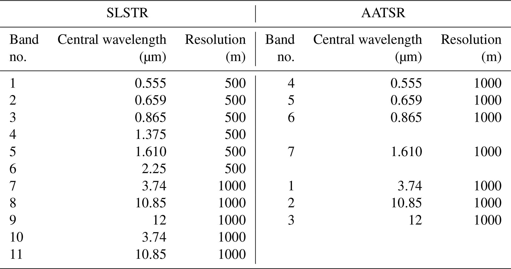
2.1 SLSTR instrument
After the loss of Environmental Satellite (Envisat) on 12 April 2012, the European Space Agency (ESA) launched Sentinel-3A and Sentinel-3B in February 2016 and April 2018, respectively. As the successor of Advanced Along-Track Scanning Radiometer (AATSR) on board Envisat, Sentinel satellites take the SLSTR instrument. The SLSTR instrument has similar characteristics to AATSR (see Table 1 for details). The instrument has nine spectral bands in the visible and infrared spectral range. It also has dual-view observation capability with swath widths of 1420 and 750 km for nadir and oblique directions, respectively. The SLSTR and AATSR dual-view observations of the Earth's surface make surface bidirectional reflectance distribution function (BRDF) effect estimation possible, which is widely used to retrieve both surface and atmospheric geophysical parameters (Popp et al., 2016). Besides the heritage of AATSR, some new features (wider swath, new spectral bands and higher spectral resolution for certain bands) have been included in SLSTR instrument (https://sentinel.esa.int/web/sentinel/technical-guides/sentinel-3-slstr/instrument, last access: 13 June 2021).
2.2 Ground-based measurements
The validation of satellite-derived snow properties is challenging due to (i) limited available field-based measurements and (ii) the difficulties of spatial–temporal collocation between satellite observations and field-based measurements because of cloud coverage. This paper focuses on the Sentinel-3a satellite for the periods of February 2016 (launch month of Sentinel-3a) and December 2020. The field-based measurements from both permanent sites and campaign sites for the focal time period are collected. Figure 1 shows the geographic distribution of the validation sites. The site names used in this paper are listed near each site. Since XBAER retrieves SGS, SPS and SSA simultaneously, the SnowEx campaign, which provides the three parameters as well, will be introduced in detail first.
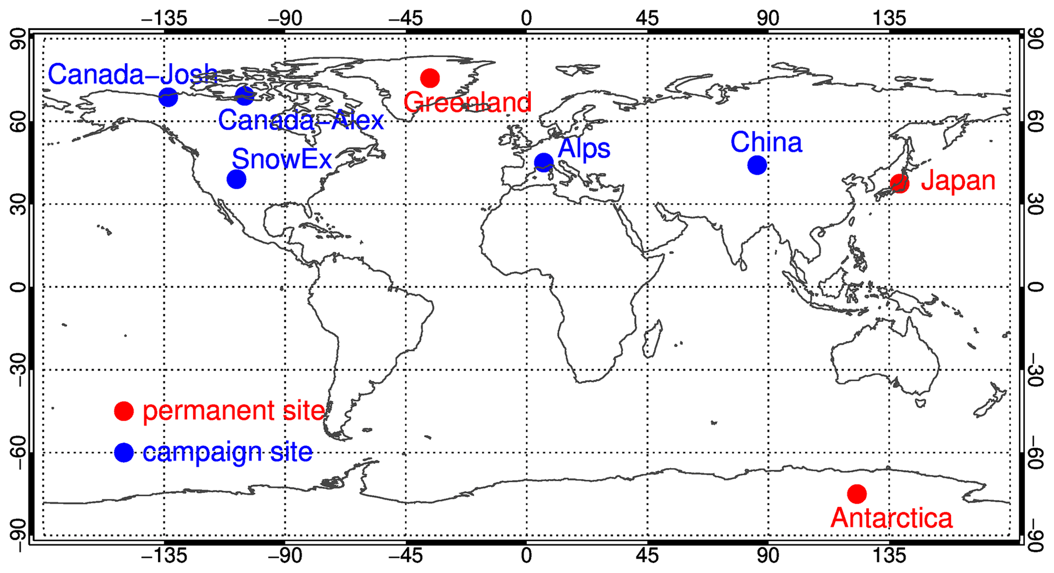
Figure 1Geographic distribution of the validation sites. The colors represent the type of each site, and the site name used in this paper is indicated near each site.
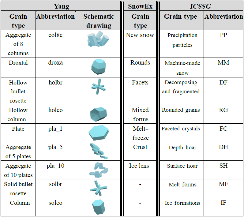
The National Aeronautics and Space Administration (NASA) established a terrestrial hydrology program (SnowEx mission) in order to better quantify the amount of water stored in snow-covered regions (Kim et al., 2017). The measurements for the first year (2016–2017) were carried out during February 2017 (between 8 and 25 February 2017) at Grand Mesa and the Senator Beck Basin in Colorado (hereafter referred to as SnowEx17) (see Fig. 2a) (Elder et al., 2018). Grand Mesa is a forest region covered by relatively homogeneous snow cover with an area size similar to airborne instrument swath widths (Brucker et al., 2017) (see Fig. 2c). The Senator Beck Basin site has complex topography and is covered by snow. The campaign used more than 30 remote sensing instruments, and most of the instruments are from the NASA except some instruments such as ESA's radar (Kim et al., 2017). The snow pit measurements provide information on snow grain size and type/shape, stratigraphy profiles, and temperatures with certain information about surface conditions (e.g., snow roughness) (Rutter et al., 2018). The SnowEx17 campaign provides seven different shapes (new snow, rounds, facets, mixed forms, melt–freeze, crust and ice lens). Table 2 lists both the SnowEx17-measured snow grain shapes and SPSs defined in Yang et al. (2013). The SPSs defined by ICSSG are also listed in the table, and the possible linkage between Yang et al. (2013) SPS and ICSSG SPS (named SPS similarity) will be discussed later. The measurements have been publicly released at http://nsidc.org/data/snowex (last access: 13 June 2021). The data were collected in SnowEx20 for the period of 27 January and 12 February 2020.
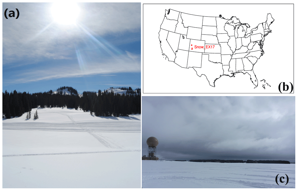
Figure 2Photos taken during the SnowEx campaign. (a) An overview of the campaign environment around the Senator Beck Basin site. (b) Location of the SnowEx campaign (red rectangles). (c) An overview of the campaign environment around the Grand Mesa site. (Credit: Roy A. Langlois and Lisa Brucker at the National Snow and Ice Data Center, University of Colorado, Boulder.)
The measurements over Greenland are obtained by the EastGRIP team over 75.63∘ N, 36.004∘ W. Detailed information about the site can be found at https://eastgrip.org (last access: 13 June 2021). The data have been used to validate the SGS and SSA derived from OLCI (Kokhanvosky et al., 2018). The same dataset, covering the period of May 2017 and August 2018 is used in this paper. SGS or SSA is calculated using the relationship between SSA and SGS if SSA or SGS is not measured.
The SSA measurements at Nunavut, northern Canada (69.20∘ N, 104.80∘ W), were obtained using the instrument described by Montpetit et al. (2012). The observation period covers April 2018.
The SPS and SSA measurements around Inuvik, Northwest Territories of Canada (68.73∘ N, 133.49∘ W), cover the period of November 2018–March 2019. There were three deployments, the freeze-up period (November 2018), the storm input period (January 2019) and the metamorphosis period (March 2019) (King et al., 2019).
The SSA measurements above the French Alps (45.04∘ N, 6.41∘ W) were collected in the snow seasons during 2016–2018 (Tuzet et al., 2020). The measurements for the 2016–2017 period provide SSA profile information with a vertical resolution of 3 cm using the DUFISSS instrument (Gallet et al., 2009). For the period of 2017–2018, the measurements were obtained with a vertical resolution of 6 cm using the Alpine Snowpack Specific Surface Area Profiler (Libois et al., 2014). The uncertainty is estimated to be 10 %.
The SGS measurements were obtained over Nagaoka, Japan (37.41∘ N, 138.88∘ W) (Yamaguchi et al., 2019; Avanzi et al., 2019). The observations during January 2017–March 2018 are used in this paper.
The SGS measurements were obtained over Xinjiang province during a different period (Chen et al., 2020); the dataset around the site (44.146∘ N, 85.848∘ E) for the period November 2018–November 2019 is used in this paper.
The SSA measurements at Dome C (75∘ S, 123∘ E) in Antarctica cover the period of 2016–2018, and the accuracy of the measurements is better than 15 % (Picard et al., 2016). The data were collected using a self-designed and assembled instrument, named Autosolexs, which can be used to measure the snow properties for several years under the harsh environment.
Table 2Snow grain type (shape) provided by Yang et al. (2013), in situ measurements in the SnowEx campaign and by ICSSG. Please note here the grain type by Yang et al. (2013) measured in SnowEx and provided by ICSSG given in the same line have no 1:1 linkage.
2.3 Aircraft observations
During the Polar Airborne Measurements and Arctic Regional Climate Model Simulation Project (PAMARCMiP) campaign held in March and April 2018, ground-based and airborne observations of surface, cloud and aerosol properties were performed near the Villum Research Station (North Greenland). One of the most important objectives of the PAMARCMiP 2018 campaign was to quantify the physical and optical properties of snow, sea ice and the atmosphere (Egerer et al., 2019; Nakoudi et al., 2020). Airborne spectral irradiance measurements by the Spectral Modular Airborne Radiation Measurement System (SMART) on board the Polar 5 research aircraft operated by the Alfred-Wegener-Institut were used to derive snow grain sizes along the flight track. The SMART provides solar up- and downward spectral irradiances in the range between 0.4–2.0 µm. The optical inlets are actively horizontally stabilized with respect to aircraft movement (Wendisch et al., 2001) within 5∘ pitch and roll angles. In particular, for high solar zenith angles (SZAs) as presented during PAMARCMiP (about an 80∘ SZA), misalignment of the optical inlets implies significant measurement uncertainties (Wendisch et al., 2001). Further uncertainties are related to the spectral and radiometric calibration, as well as to the correction of the cosine response which sums to a total wavelength-dependent uncertainty (1 sigma) for the irradiances ranging between 3 % and 14 % (Jäkel et al., 2015). The derivation of the surface albedo from aircraft observations requires atmospheric corrections due to the atmospheric attenuation and scattering by gases and aerosols. Therefore an iterative method to correct for these effects was applied according to the procedure described by Wendisch et al. (2004). The retrieval of the snow grain sizes is based on the method described in Carlsen et al. (2017) which uses a modified approach presented by Zege et al. (2011).
3.1 Cloud screening
The algorithm synergistically uses SLSTR and OLCI data to identify clouds over the snow surface. The criteria for cloud screening over snow using SLSTR and OLCI measurements can be found in Istomina et al. (2010) and Mei et al. (2017), respectively. Short summaries of Istomina et al. (2010) and Mei et al. (2017) are presented below, and more details can be found in the original publications. The algorithm proposed by Istomina et al. (2010) for the SLSTR instrument utilizes spectral behavior differences at SLSTR visible and thermal infrared channels, and this algorithm was updated later by Jafariserajehlou et al. (2019). Relative thresholds are determined based on radiative transfer simulations under various atmospheric and surface conditions. The method proposed by Mei et al. (2017b) for the OLCI instrument uses different cloud characteristics: cloud brightness, cloud height and cloud homogeneity. The TOA reflectance at 0.412 µm, the ratio of TOA reflectance at 0.76 and 0.753 µm, and the standard deviation of TOA reflectance at 0.412 µm are used to characterize cloud brightness, cloud height and cloud homogeneity, respectively. A pixel is identified as a cloud-free snow pixel when both SLSTR and OLCI identify it as a cloud-free snow pixel. Identified clouds can be surrounded by a so-called “twilight zone” (Koren et al., 2007), which can extend more than 10 km from a cloud pixel to a cloud-free area. The surrounding 5×5 pixels of an identified cloud pixel will be marked as a cloud to avoid the twilight zone effect. A more detailed description of this cloud screening method can be found in Mei et al. (2020a). Additionally, TOA reflectance at 0.55 µm is required to be higher than 0.5 to avoid dark ice and dirty snow.
3.2 Atmospheric correction
Due to the low atmospheric aerosol loading over the Arctic snow-covered regions (e.g., Greenland), atmospheric correction using path radiance representation (Chandrasekhar, 1950; Kaufman et al., 1997) can provide accurate estimation of surface reflection even under relatively large SZAs (Lyapustin, 1999). The TOA reflectance at selected channels (0.55 and 1.6 µm) is described by the path radiance representation (Chandrasekhar, 1950; Kaufman et al., 1997) as
where is the TOA reflectance calculated assuming a black surface (surface reflectance equals 0) under a viewing zenith angle (VZA), solar zenith angle (SZA) and relative azimuth angle (RAA) of θ, θ0 and φ. τ and AT are aerosol optical thickness (AOT) and aerosol type (Mei et al., 2017a). is the total (diffuse and direct) transmittance from the sun to the surface and from surface to the satellite; s(τ,AT) is spherical albedo; A is Lambertian surface albedo. The spherical albedo is the fraction of the incident solar radiation diffusely reflected over all directions (albedo of an entire planet). The Lambertian surface albedo is defined as the ratio of reflected to incident flux. The atmospheric correction is performed based on the following equation:
The atmospheric correction is based on the look-up table (LUT) pre-calculated using the radiative transfer code SCIATRAN (Rozanov et al., 2014). The radiative transfer calculations were performed assuming AOT values provided by Modern-Era Retrospective Analysis for Research and Applications (MERRA) simulations, and aerosol type was defined as weakly absorbing according to a previous investigation (Mei et al., 2020b).
3.3 XBAER algorithm
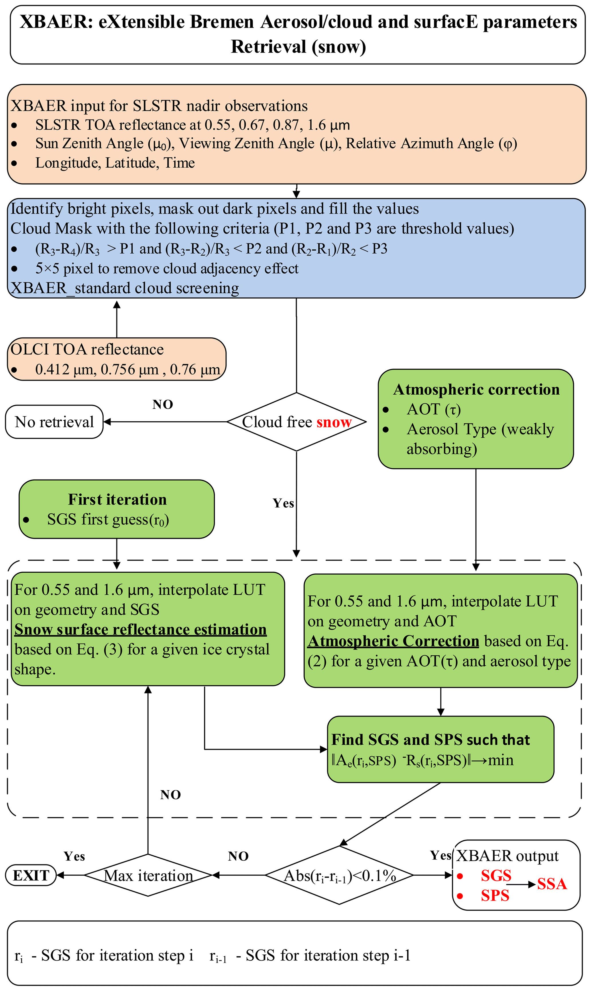
The theoretical background of the retrieval algorithm is given in Sect. 4 of the companion paper. The XBAER algorithm consists of three stages to derive SGS, SPS and SSA: (1) derivation of SGSs for each predefined SPS, (2) selection of the optimal SGS and SPS pairs for each scenario, and (3) calculation of SSA for each retrieved SGS and SPS. This section describes some implementation details such as the selection of the first guess for the retrieval parameters and the flowchart of the algorithm.
A reasonable first-guess value for the iteration process can significantly reduce the computation time, which is important for retrievals of atmospheric and surface properties over large geographic and temporal scales with different instrument spatial resolutions. The first guess of SGS in the XBAER algorithm is obtained employing the semi-analytical snow reflectance model (Kokhanovsky and Zege, 2004; Kokhanovsky et al., 2018). Details of using this model to derive SGS can be found in Lyapustin et al. (2009). Due to the different band settings in MODIS and SLSTR (SLSTR has no 2.1 µm channel like MODIS), one non-absorption channel (0.55 µm) and one absorption channel (1.6 µm) are used in our SLSTR retrieval algorithm.
Figure 3 shows the flowchart of how XBAER derives SGS, SPS and SSA. The flowchart includes pre-processing of cloud screening using the synergy of OLCI and SLSTR and the atmospheric correction using MERRA providing AOT and a weakly absorbing aerosol type. The SGS and SPS are obtained using the LUT-based minimization routine. SSA is then calculated using the retrieved SGS and SPS.
Greenland is the largest ice-covered land mass in the Northern Hemisphere and the biggest cryospheric contributor to the global sea-level rise (Ryan et al., 2019). XBAER-derived SGS, SPS and SSA over Greenland enable a good understanding of the retrieval accuracy with a large and representative geographic scale. Kokhanovsky et al. (2019) reported that July is an optimal month to analyze satellite-derived snow properties over Greenland because Greenland has a strong snow particle metamorphism process (SPMP) due to higher temperatures in July (Nakamura et al., 2001). The SPMP, affected strongly by temperature, is a dominant factor for the variabilities in SGS, SPS and SSA (LaChapelle, 1969; Sokratov and Kazakov, 2012; Saito et al., 2019). Snow particle size increases dramatically and the ice crystal particles are compacted in the strong SPMP (Aoki et al., 1999; Nakamura et al., 2001; Ishimoto et al., 2018). Figure 4 shows an example of the XBAER-derived SGS on 28 July 2017 from SLSTR, XBAER first guess, and its comparison with the same scenario from the MODSCAG product (Painter et al., 2009). Here we chose MODIS on Aqua rather than MODIS on Terra to avoid the impact of instrument degradation of MODIS on Terra (Lyapustin et al., 2014). The visualization of XBAER-derived SGS is shown to be between 10 and 500 µm. The XBAER first guess has in general a low value (Lyapustin et al., 2009) as compared to XBAER and MODSCAG results. The XBAER- and MODSCAG-derived SGSs show good agreement on the geographic distribution. The slight difference in cloud-covered regions (white parts) is explained by the different overpass time between SLSTR and MODIS. Both algorithms demonstrate that SGSs in central Greenland are smaller than those at coastline regions. This is attributed to the geographic distribution of surface temperature over Greenland. In particular, central Greenland has a significantly higher elevation, and the impacts of imperfect atmospheric correction on retrieved snow properties are ignorable. The lower temperature under higher-elevation regions has a weaker SPMP, producing more irregular SPS. The opposite situation is the case in the coastline regions over Greenland. Since Fig. 4 is composited by three different SLSTR orbits, the geometrically shaped features in eastern Greenland are caused by the effective Lambertian albedo assumption in the XBAER algorithm. This assumption introduces additional bias under large viewing zenith angle conditions, which occurs at the edge of each SLSTR orbit.
Figure 5 shows XBAER-retrieved SGS, SPS and SSA for 28 July 2017. Since there are no available products of SPS and SSA from MODSCAG, it is a great challenge to make a similar comparison to that in the case of SGS. Fortunately, campaign-based and laboratory investigations provide valuable information on typical snow shapes at different times and locations with a wide range of atmospheric conditions. According to Kikuchi et al. (2013), the typical SPSs in the polar regions include column crystal (e.g., solid column, bullet-type crystal) with SGSs of about 50 µm for solid column and between 100 and 500 µm for bullet type, and the germ of ice crystal group with SGSs of less than 50 µm. Saito et al. (2019) pointed out that SPSs of fresh snow in the polar regions are typically a mixture of irregular shapes such as column and plate-like. Ishimoto et al. (2018) found that aged snow can have an aggregate structure. The optical properties of small ice crystal particles in aged snow may be well-characterized by granular/roundish shapes, while SPSs tend to be irregular or severely roughened shapes during the SPMP (Ishimoto et al., 2018). Pirazzini et al. (2015) investigated the impact of ice crystal sphericity on the estimation of snow albedo and found droxtal is a reasonable assumption to take ice particle non-sphericity into account. The above conclusions can be used as a qualitative reference to understand the satellite-derived SPS. In the meantime, a large proportion of ice sheet melts during the warm July, which unequivocally leads to rounded coarse grains very quickly. According to Fig. 5, central Greenland is largely covered by small particles with a roundish/droxtal shapes, while coastline regions are covered by particles with aggregated shapes (aggregate of 8 columns, aggregate of 5 plates, aggregate of 10 plates) with large particle sizes, which is essentially attributed to the different SPMPs over different regions of Greenland. Bullet-type crystal (solid bullet rosette) occurred with SGSs of about 100 µm. The examples shown in Fig. 5 can be reasonably explained by previous publications (Kikuchi et al., 2013; Pirazzini et al., 2015; Ishimoto et al., 2018; Saito et al., 2019).
The geographic distribution of SSA is somehow anti-correlated with the geographic distribution of SGS, due to the definition of SSA. Most SSAs fall into the range of 10–40 m2/kg, which agrees with previous publication (Kokhanovsky et al., 2019). A change in SSA occurs especially after snowfall (Carlsen et al., 2017; Xiong and Shi, 2018). Since SSA contains information on both SGS and SPS and field measurements provide SSA, the validation of SSA can be also used as “indirect quantitative validation” of SPS, which will be quantitatively presented in the next section.
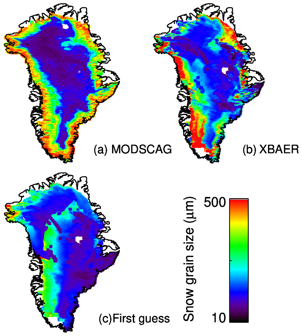
Figure 4A comparison of the MODSCAG SGS (a), XBAER-derived SGS (b) and first guess (c) over Greenland on 28 July 2017.
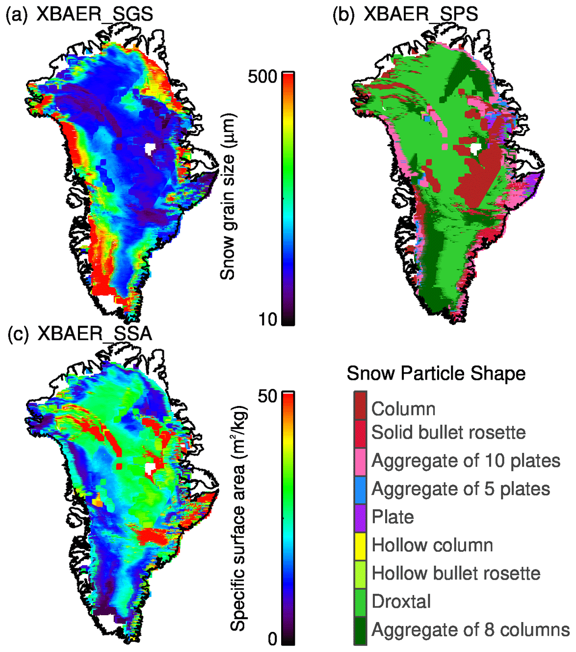
Figure 5XBAER-derived SGS, SPS and SSA over Greenland for the same scenario as in Fig. 4.
In this section, we will quantitatively validate XBAER-derived snow properties with field-measured data and aircraft measurements.
5.1 Validation using the observations of the SnowEx17 campaign
In order to have a quantitative evaluation of XBAER-derived SGS, SPS and SSA, we have collocated the SLSTR observations with recent campaign measurements provided by SnowEx17 and SnowEx20, as described in Sect. 2. Due to overpass time and cloud cover, only limited match-ups between XBAER retrievals and SnowEx17 and SnowEx20 measurements have been obtained. No match-up is obtained for SnowEx20.
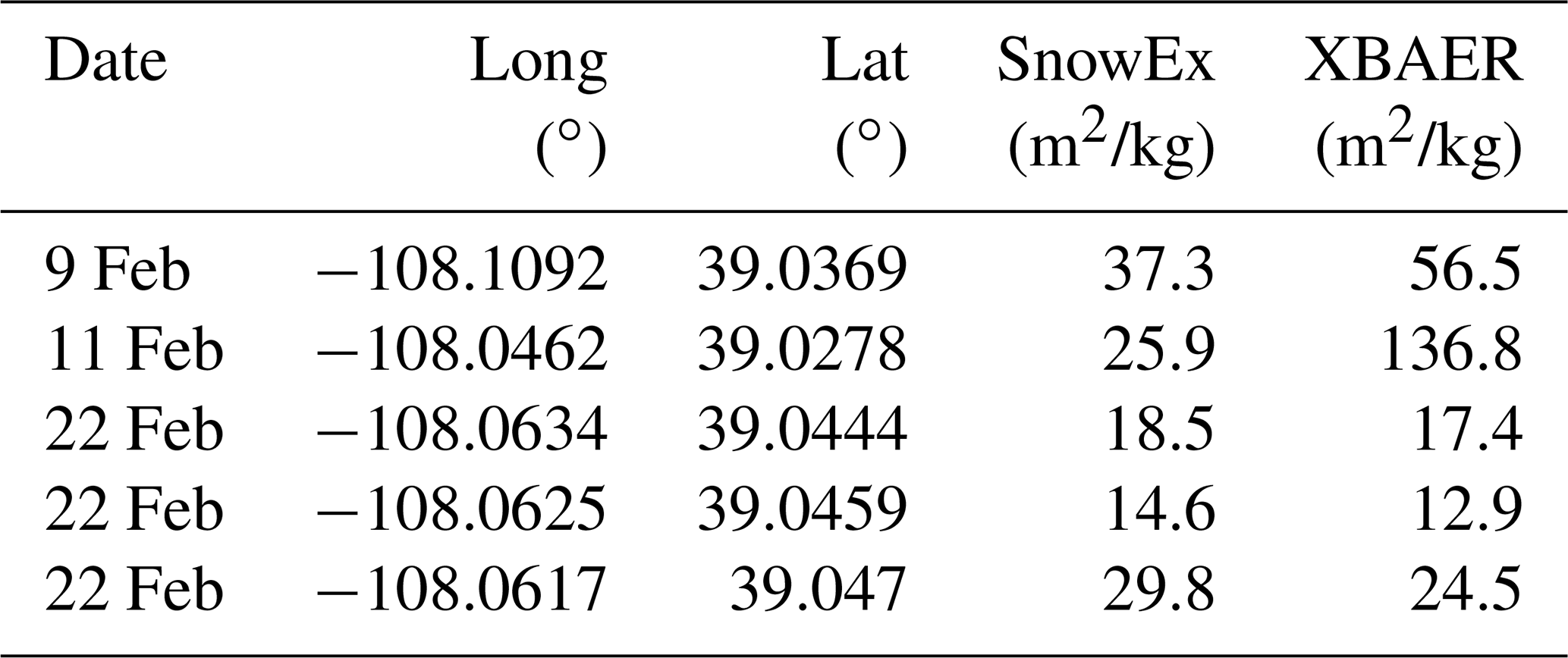
Table 3 summarizes match-up information. The first three columns in Table 3 show the observation times and locations (longitude and latitude). The fourth and fifth columns indicate the cloud conditions. Cloud conditions in Table 3 are given in three categories: cloud-free snow, cloud-contaminated snow and cloud-covered snow. These three categories are classified by the XBAER cloud identification results (see Sect. 3.1) and are illustrated by the RGB composition figures, covering the SnowEx campaign area, as presented in Fig. 6. An optically thin cloud over a melting snow layer, a thick cloud over snow and snow scenarios are presented in Fig. 6a, b and c, respectively. The cloud optical thickness (COT), estimated using the independent XBAER cloud retrieval algorithm, as presented in Mei et al. (2018), is ∼0.5 and ∼10 for 9 and 11 February, respectively.
Table 3Information of match-ups between SnowEx and SLSTR during February 2017.
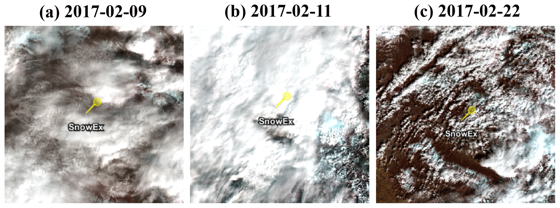
Figure 6Zoom of the RGB composition figures (created using ESA official SLSTR software SNAP) for the three selected dates presented in Table 3. The yellow point indicates the SnowEx instrument position.
Even though the synergistical use of SLSTR and OLCI provides valuable information for separating cloud and snow, the identification of an optically thin cloud above a snow layer is a great challenge due to the similar wavelength dependence of snow and cloud reflectance, especially between snow and ice cloud (Mei et al., 2020b). The identification of the cloud from an underlying snow layer in XBAER relies mainly on the O2 channel of the OLCI instrument, which provides the cloud height information (Mei et al., 2017b). Figure 7 shows the performance of XBAER cloud identification results for cloud contamination and cloud-covered snow scenarios. The red star indicates the measurement location. The zoomed-in images around the measurement site are presented in Fig. 6. XBAER cloud screening shows, in general, good performance according to the RGB visual interpretation. However, part of the thin cirrus cloud on the 9 February is not correctly avoided. For 9 February, XBAER cloud identification gives a result of clean snow while it contains a thin cloud above a snow layer. For the 11 February, XBAER has successfully detected the cloud from an underlying snow layer. For a comprehensive investigation of XBAER-derived snow properties under all snow–cloud-coupled conditions, the match-up on 11 February 2017 (shown in grey) has been manually set to “cloud-free snow”. The reason for performing the validation for different cloud conditions is that the satellite retrieval can only be performed under cloud-free conditions, while field measurements may be obtained under cloud conditions, especially when fresh snow properties are measured. Thus, the field-based measurements under full-cloud or partly cloudy conditions are still valuable in the validation process (Jeoung et al., 2020). According to the sensitivity study, cloud contamination leads to an underestimation of SGS and the overestimation of SSA, depending on the cloud fraction.
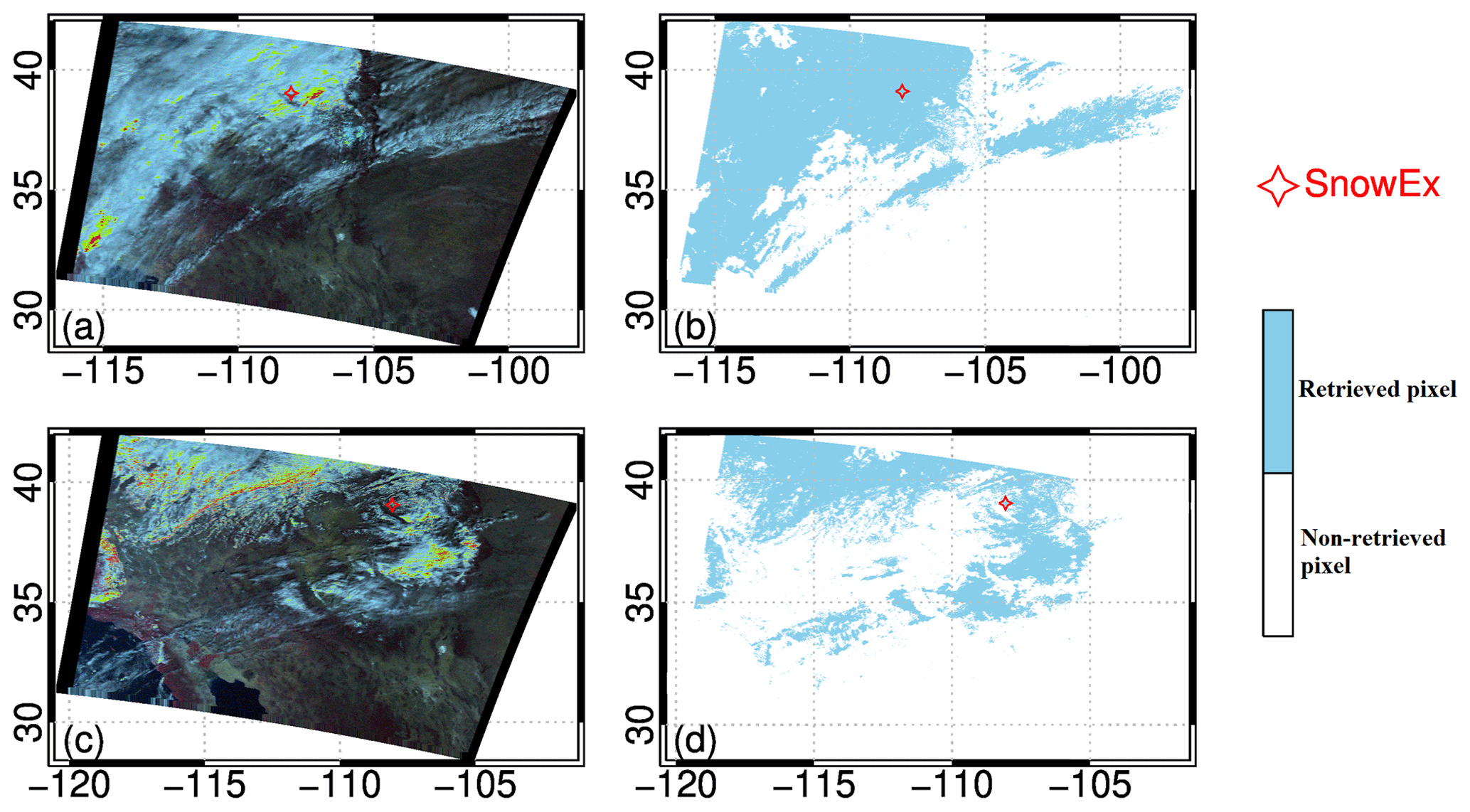
Figure 7The RGB composition (a, c) for 9 (a) and 22 (c) February when XBAER detected cloud-free snow and provided the retrieval. The XBAER cloud screening results (b, d) for the corresponding days are given in (b) and (d). “Retrieved pixel” refers to cloud-free snow. “Non-retrieved pixel” refers to the area where XBAER retrieval is not performed; this includes (1) snow-free and cloud-free, (2) cloud above snow, and (3) cloud above snow-free.
Table 4 summarizes the comparison between XBAER retrieval results, the MODSCAG product and SnowEx17 campaign measurements. The first three columns in Table 4 are the same as those of Table 3, showing the observation time and locations (longitude and latitude). The second three columns are the SnowEx17-measured SGS. Since the SnowEx17 provides the SGS profile up to a 1 m depth, the minimum (SnowEx_min), average (SnowEx_avg) and maximum (SnowEx_max) values of SGS are listed in Table 3. The last two columns are MODSCAG- and XBAER-derived SGS. For the four cloud-filter-passed match-ups, XBAER-derived SGS shows good agreement with SnowEx17 measurements, especially for the 22 February. The average absolute difference is less than 10 µm (4 % in relative difference). The relatively large SGS (≥ 250 µm) caused mainly by the warm-up on the 21 February (see the comment in Table 5, reported by campaign participators) led to a quicker snow metamorphism process, forming large ice crystal particles. MODSCAG only provides retrieval results for 9 and 11 February. The results from XBAER and MODSCAG agree well. This possibly indicates similar performance between XBAER and MODSCAG.
An underestimation is found for the first match-up on the 9 February. This is explained by the cirrus cloud contamination as presented in Fig. 11. According to an independent XBAER cloud retrieval (Mei et al., 2018), the COT is ∼ 0.5; cloud contamination with a COT of 0.5 introduces a ∼ 30 % underestimation according to Fig. 11 in the Part 1 companion paper. So for SGS = 100 µm, provided by SnowEx, XBAER is expected to have a theoretically retrieved SGS of ∼ 70 µm, while a value of 78.2 µm is obtained from the real satellite retrieval. In order to further confirm this negative bias feature caused by cloud contamination, the 11 February retrieval (a snowstorm at the measurement site is reported by campaign participators), although filtered by the XBAER cloud screening routine, is forced to retrieve the fully cloud-covered scenario as a cloud-free case. According to the theoretical investigations presented in the Part 1 companion paper, for COT ≥ 5, the XBAER algorithm retrieves the cloud effective radius rather than SGS. The retrieved ice crystal size depends on the cloud effective radius of the cloud above the underlying snow layer. The independent XBAER cloud retrieval provides an SGS value of ∼ 38, while 32.3 µm is obtained by the XBAER snow retrieval, for a reference value of 100 µm as provided by SnowEx17 measurement. This is consistent with a typical ice cloud effective radius (King et al., 2013; Mei et al., 2018) under a snowstorm condition.
Table 4The comparison between SnowEx SGS measurements, XBAER- and MODSCAG-retrieved SGS during February 2017.
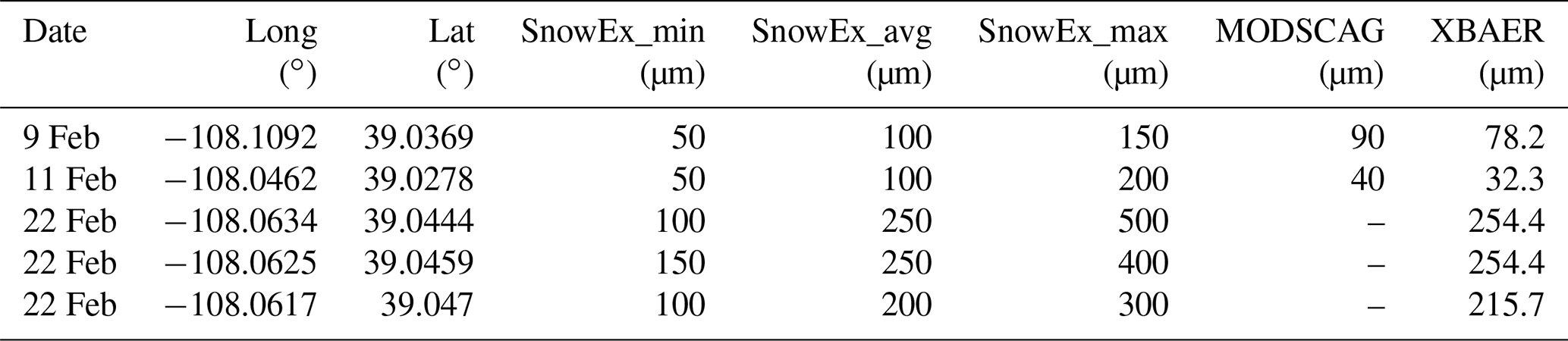
Table 5 shows the same match-up information as in Table 4 but for SPS. We would like to highlight again that the SPSs proposed by Yang et al. (2013) are used for the radiative transfer calculation. From a single-ice-crystal point of view, those shapes are very unlikely to occur exactly in reality. This is similar to the issue in field measurements. In field-based measurements, a spherical-shape assumption is widely used (e.g., the calculation of SSA from SGS); however, a pure spherical shape is also very unlikely to occur in natural snow. To have a reasonable comparison between satellite-derived SPS and field-measured SPS, the quantitative information of “roundish” or “irregular” shapes from both satellite and field measurement communities may be an option. Under this comparison strategy, a “droxtal” shape derived from satellite observation is somehow identical with a “spherical shape” in field measurement.
The second and third columns in Table 5 show SnowEx17-measured and XBAER-derived SPS. The abbreviations of the SPS are listed in Table 2. The fourth–sixth columns are the temperature, wetness of snow and the comments provided by campaign participants, respectively. Previous publications show that ice cloud and fresh snow are best described by aggregate of 8 columns (Platnick et al., 2017; Järvinen et al., 2018). Both 9 and 11 February are retrieved to be aggregate of 8 columns because both of them are affected by ice cloud. The first sample on 22 February is reported to be aggregate of 8 columns and the observation of SnowEx17 is fresh snow. The SPS of the second sample on 22 February is “facet” while XBAER says droxtal, indicating possible linkage between XBAER-derived droxtal and field-measured facet. It is interesting to compare the SPS for the third sample on 22 February. The SPSs are round and aggregate of 8 columns for the SnowEx17 measurement and XBAER retrieval, respectively. The atmospheric condition is reported to be “windy”, and the snow layer is wind-affected and not very well banded ice crystal. The ice crystal shape in blowing snow is likely to be irregular and aggregated (Lawson et al., 2006; Fang and Pomeroy, 2009; Beck et al., 2018), which is strongly affected by the near-surface processes (Beck et al., 2018). Snow grains may also become rounded due to sublimation in blowing snow (Domine et al., 2009). The wind blowing snow may be well-represented optically by an “aggregate-of-8-columns” shape, as retrieved by XBAER.
Table 5The comparison between SnowEx snow grain shape and XBAER-retrieved SGP during February 2017.
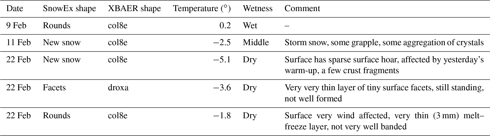
Table 6 shows the comparison of SSA. For the three cloud-free samples, the difference in XBAER-derived SSA and SnowEx17-measured SSA is 2.7 m2/kg, which is significantly smaller than what has been reported by previous publications. For instance, the differences between satellite retrievals and field measurements are reported to be 9 and ∼ 6 m2/kg in Mary et al. (2013) and Xiong and Shi (2018). An interesting case is observed for the two samples on 22 February. The SGSs show the same values for these two match-ups (both are 254.4 µm from XBAER and 250 µm from SnowEx); however, ground-based measurement shows almost 2 times the difference in SSA (29.8 vs. 14.6 m2/kg) for these two samples, which is due to the different SPSs. SnowEx shows that the SPSs are new snow and facets for these two samples, respectively. XBAER-derived SSAs are 24.5 and 12.9 m2/kg, which agrees well with SnowEx measurement. Since both SnowEx and XBAER provide very similar SGSs (250 µm vs. 254.4 µm), the agreement of SSA indicates that XBAER-derived aggregate of 8 columns is comparable to “new snow”, while XBAER-derived droxtal is somehow “identical” to facets in SnowEx. Cloud contamination introduces an overestimation of SSA, especially for 11 February. According to the investigation from the companion paper, for reference SSAs of 37.3 and 25.9 m2/kg, SSA is expected to be ∼ 65 and > 100 m2/kg for cloud contamination with COT ∼ 0.5 and 10, respectively. The real satellite retrieval values are 56.5 and 136.8 m2/kg.
Table 6The comparison between SnowEx SSA and XBAER-retrieved SSA during February 2017.
The above validation for the retrieval of SGS, SPS and SSA using the XBAER algorithm, although with limited samples, indicates the consistency of the sensitivity study from the Part 1 companion paper and the retrieval results in Part 2, as presented in this section.
5.2 Validation using the observations of other campaigns
For comprehensive validation, we have analyzed the rest of the sites besides the SnowEx site. The comparison is performed based on the daily mean observation following the method from Wiebe et al. (2011). We have restricted the SGS in the range of 0–300 µm, while the SSA is in the range of 0–100 m2/kg. Thus there may be a slightly difference in the number of total match-ups for SGS and SSA. Figure 8 shows the comparison between XBAER-derived snow properties and field-based measurements. Both SGS and SSA show good correlation between XBAER-derived and field-based measurements, with correlation coefficients larger than 0.85. A clear underestimation of SGS, especially for large SGS values, is observed. This can also been seen from the slope of the regression (slope = 0.67). XBAER shows good agreement with field-based measurements, especially for SGSs smaller than 150 µm. The underestimation occurs mainly over regions with complicated surface conditions and/or large aerosol loading. In general, we can see larger deviation from the 1:1 line when AOT values are larger. This agrees with a major finding in the Part 1 companion paper, that is, aerosol contamination introduces underestimation of SGS. For instance, large AOT values can be seen over China, while strong underestimation of SGS is also observed. For the Alps and two Canadian (Canada-Alex, Canada-Josh) sites, the AOT values are fairly low; the underestimation may be explained by the strong surface inhomogeneity (possibly due to different surface types in one satellite pixel). For sites Greenland and Antarctica, where AOT values are low and the surface is covered mainly by snow, XBAER shows good performance. This can be confirmed by the root mean square error (RMSE) values. The RMSE values in Fig. 8 are calculated only for site Greenland and Antarctica, to avoid the large outliers over other sites (please note other sites provide quite a limited number of match-ups; see Fig. 9). The RMSE value is 12 µm. The comparison between XBAER-derived and field-measured SSA shows no significant under-/overestimation (slope = 1) with a correlation coefficient R = 0.93. XBAER-derived SSAs are, in general, larger than field-based measurements. This can be explained by the use of different SPS assumptions. In the XBAER algorithm, for the match-ups shown in Fig. 8, most SPSs are non-convex, while the convex SPS is used for field-measured values. We recall that for the same SGS, a non-convex particle leads to a larger SSA, compared to a convex particle. The impact of aerosol contamination, compared to surface conditions, seems to play a major role in the observed overestimations.
The potential linkage between XBAER-derived SPS and field-measured SPS is also presented in Fig. 8. This is named SPS similarity in this paper. The SPS similarity is defined as the ratio of the match-up number for a given SPS pair (XBAER-retrieved SGS from Yang et al., 2013, field-measured ICSSG SPS) to the total match-up number. The higher the SPS similarity, the higher chance this SPS pair may occur in reality, indicating the higher possibility that the retrieved Yang et al. (2013) SPS may have a closer relationship with ICSSG SPS. According to Fig. 8, we can see that aggregate of 8 columns, solid bullet rosette and column show stronger linkage with the rounded grains while droxtal, plate and column show stronger linkage with the faceted crystals. This may lead to an imperfect and highly uncertain linkage between XBAER-derived SPS and the ICSSG SPS. Aggregate SPS in XBAER is likely to be matched with rounded gains, while single SPS in XBAER is possibly linked to faceted crystals. There is also possible linkage between XBAER SGS and ICSSG SPS, for instance, aggregate of 8 columns and plate with precipitation particles, solid bullet rosette with depth hoar, and droxtal and plate with surface hoar. The above linkage also indicates that aggregate of 8 columns (linked to rounded grains and precipitation particles) may represent fresh snow, while droxtal (linked to faceted crystals and surface hoar) may represent aged snow. This agrees with the previous analysis over Greenland.
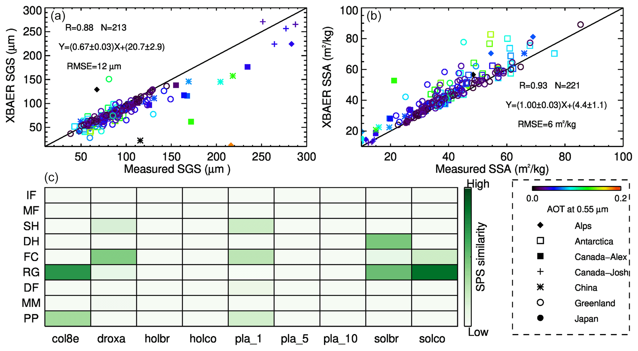
Figure 8Validation of XBAER-derived SGS, SPS and SSA. The upper panels show the scatterplots for SGS and SSA, while the lower panel shows the relationship of SPS between XBAER and ICSSG. The match-ups for SGS and SSA are distinguished by sites and the AOT. The correlation coefficient (R), number of match-ups (N), regression equation and RMSE are given. The relationship of SGS between XBAER and ICSSG (named SPS similarity) is defined as the ratio of the number of given match-ups to the total match-ups.
Figures 9 and 10 show the time series of SGS and SSA over each site. We can see that sites Greenland and Antarctica provide most of the match-ups. Both SGS and SSA show good agreement between XBAER-derived and field-measured values over these two sites. For SGS, the correlation coefficients are 0.85 and 0.89 and the RMSEs are 14 and 9 µm, respectively. For SSA, those values are 0.84 and 0.89 for the correlation coefficient and 8 and 7 m2/kg for RMSE, respectively. Although the other sites provide limited match-ups, they still give helpful information for the understanding of impacts of surface and atmospheric conditions. In general, sites China and Japan show large AOT values, leading to underestimation of SGS and overestimation of SSA. For the two Canadian sites (Canada-Alex, Canada-Josh), the under-/overestimation of SSA and SGS may largely be explained by the surface condition. The Alps site seems to be affected by both surface and atmospheric impacts.
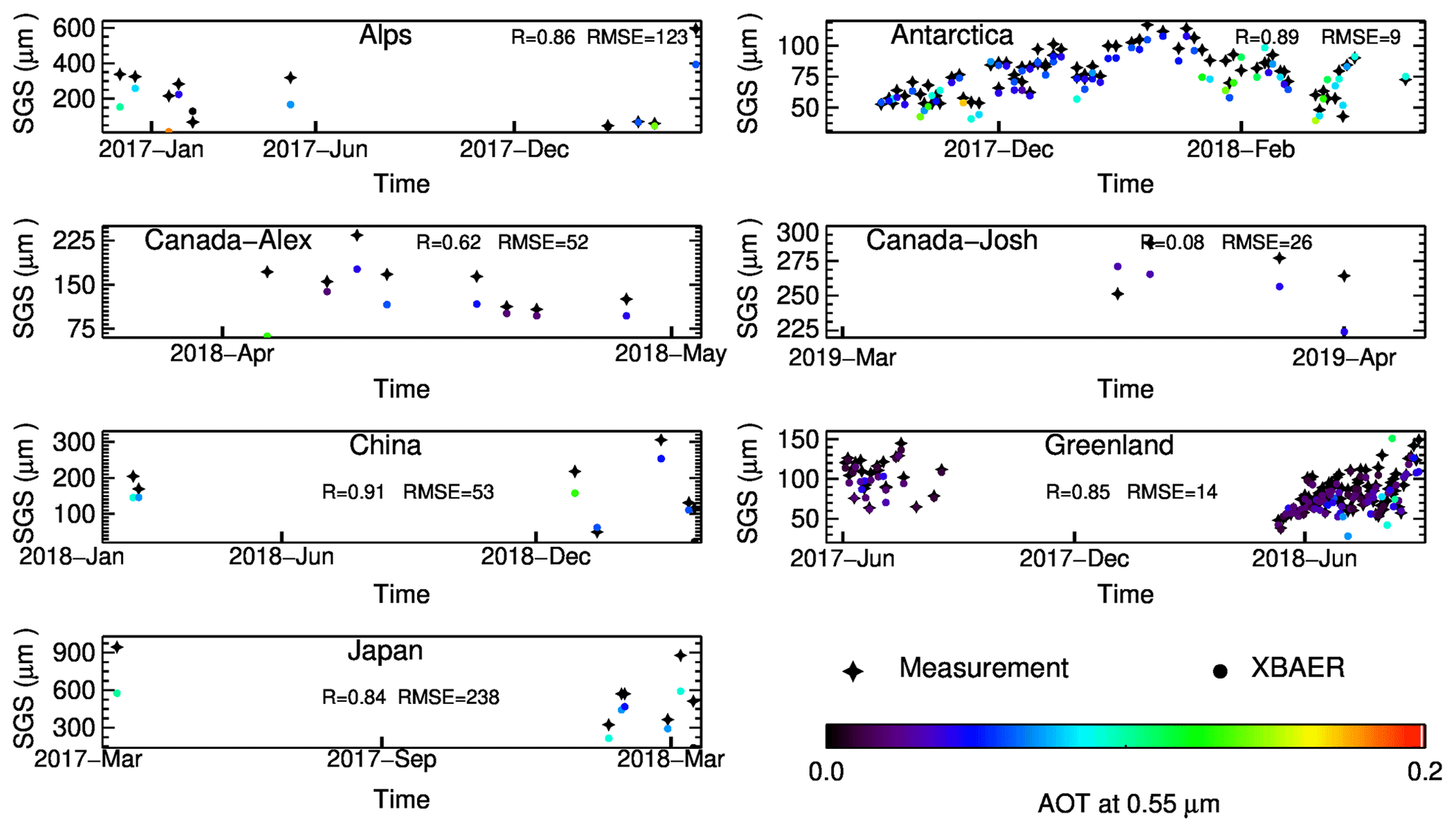
Figure 9Time series of XBAER-derived and field-measured SGS for each site. The match-ups for SGS are distinguished by the AOT values. The correlation coefficient (R) and the RMSE (µm) are given.
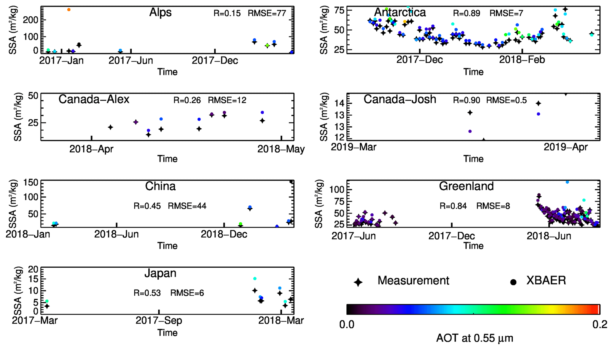
Figure 10Time series of XBAER-derived and field-measured SSA for each site. The match-ups for SGS are distinguished by the AOT values. The correlation coefficient (R) and the RMSE (m2/kg) are given.
5.3 Validation using the observations of aircraft campaign
The optical snow grain size over Arctic sea ice was derived from airborne SMART measurements as described in Sect. 2.3. Figure 11a shows the retrieved grain size along the flight track (black-encircled area) taken on 26 March 2018 between 12:00 and 14:00 UTC north of Greenland. During this period of cloudless conditions, a Sentinel-3 overpass (12:29 UTC) delivered SGS data based on the XBAER algorithm as displayed in the background of this map with a 1 km spatial resolution. In general, lower SGSs were observed by both methods in the vicinity of Greenland, while in particular in the northeast region of the map (dashed red circle in Fig. 11a) SGS values of up to 350 µm were derived from the aircraft albedo measurements. The XBAER algorithm also reveals higher values in this region. For a direct comparison, XBAER data were allocated to the time series of the SMART measurements along the flight track. Afterwards all successive SMART data points assigned to the same XBAER location were averaged to compile a joint time series of both datasets as displayed in Fig. 11b. Overall a correlation coefficient of R = 0.82 and an RMSE of 12.4 µm were derived, where SMART (mean SGS 165 ± 40 µm) generally shows larger grain sizes than XBAER (mean SGS 138 ± 21 µm). The course of the SGS follows a similar pattern for both methods, with the largest deviations when the aircraft measured in the area depicted by a dashed red circle in Fig. 11a. The corresponding time periods are indicated by the light-red-shaded area. Camera observations along the flight track have revealed an increase in surface roughness in this area. Note that the flight altitude varied for the flight section shown in Fig. 11a. Due to the low sun (SZA ), such a non-smooth surface produces a significant fraction of shadows which lowers the measured albedo. Consequently, the retrieved SGS is affected in particular for the lowest flight section when SMART collects the reflected radiation with a high spatial resolution. This might explain why the deviation of the retrieved SGS values in this area are largest around 13:00 UTC when flight altitude was in the range of 100 m.
The SGS retrieval based on the algorithm suggested by Zege et al. (2011) and Carlsen et al. (2017) gives the optical radius of the snow grains such that the SSA can be derived applying Eq. (A1) from the companion paper. The map of the SSA (Fig. 11c) reflects a similar pattern to that observed for the SGS, showing an inverse behavior to that depicted in Fig. 11a. On average, XBAER (mean SSA 24 ± 3 m2/kg) and SMART (mean SSA 21 ± 5 m2/kg) agree within the 1σ standard deviation. The correlation of SSA between XBAER and SMART is similar to that for the SGS with a correlation coefficient R of 0.81 and RMSE of 2.0 m2/kg. A comprehensive comparison between XBAER and SMART is given in Jäkel et al. (2021).
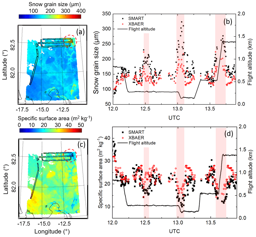
Figure 11(a) Map of SGS retrieval results from Sentinel measurements in the north of Greenland from 26 March 2018. The black-encircled area represents the SMART retrievals of the SGS along the flight track. The dashed red circle marks a region with increased surface roughness. (b) Time series of both retrieval datasets adapted to the aircraft flight path. Periods matching with the circled area in (a) are shaded in light red. Panels (c) and (d) are similar to (a) and (b) but for SSA. Additionally, the flight altitude is given.
Since XBAER is also designed to support the MOSAiC campaign on an Arctic-wide scale (Mei et al., 2020c), it is important to have an overview of how snow properties look on an Arctic-wide scale for the existing campaign. Figure 12 shows the SGS, SPS and SSA geographic distribution over the whole Arctic for 26 March 2018. Northern Greenland, North America and central Russia show large snow particles, especially over North America. And the SPS shows more diversity in lower latitudes compared to the central Arctic, indicating a stronger SPMP. An aggregated shape such as aggregate of 8 columns is the dominant shape in the central Arctic, while column is one of the dominant shapes in lower latitudes. SSA shows large values in the lower-latitude Arctic (northern Canada, southern Greenland, western Norway, southern Finland, northern Russia), while the values are smaller in the central Arctic.
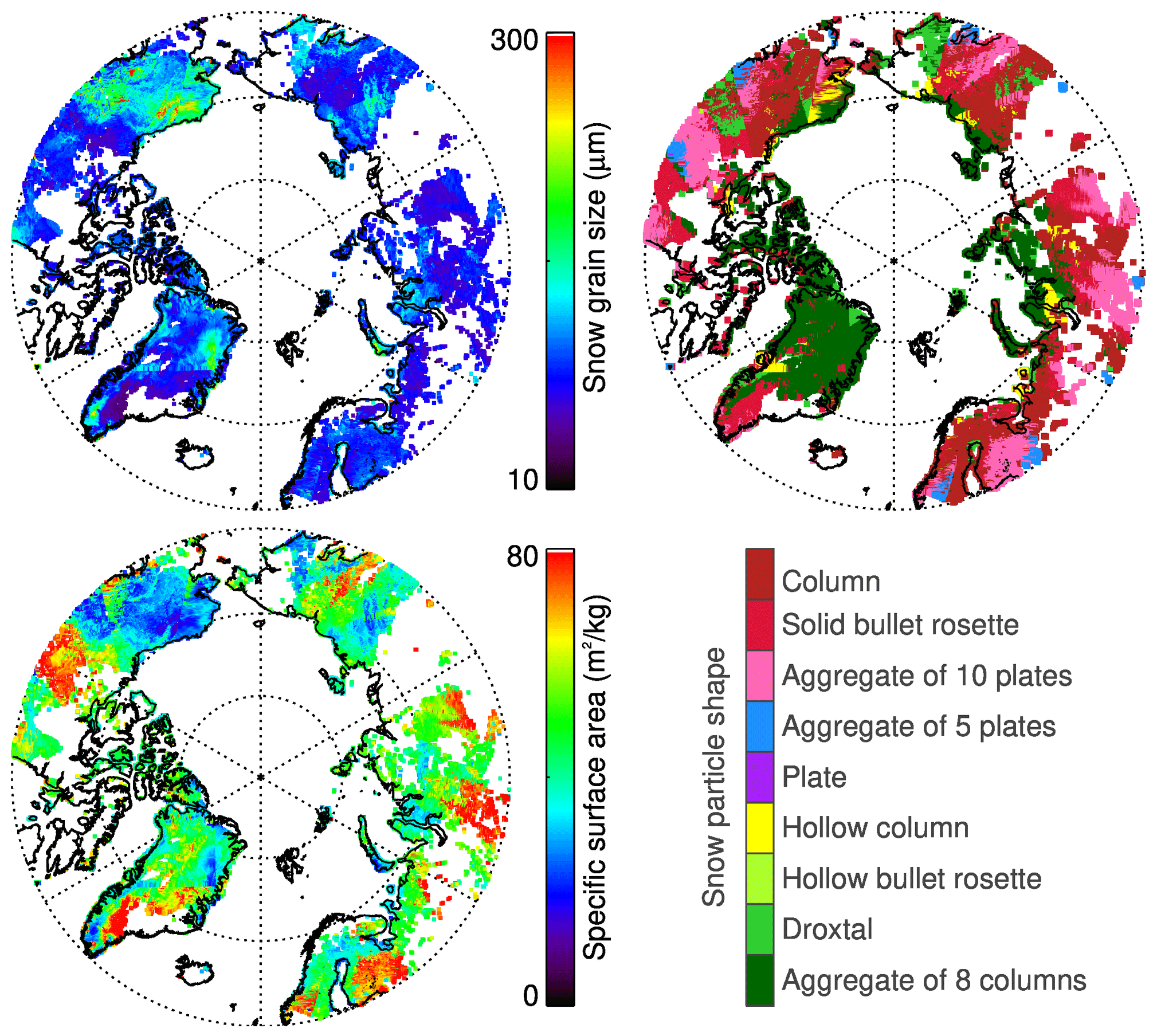
Figure 12The distribution of XBAER-derived SGS, SPS and SSA over the whole Arctic for 26 March 2018.
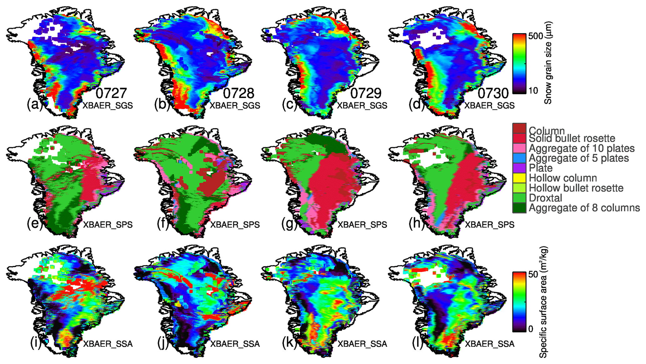
Figure 13XBAER-derived SGS, SPS and SSA over Greenland during 27–30 July 2017.
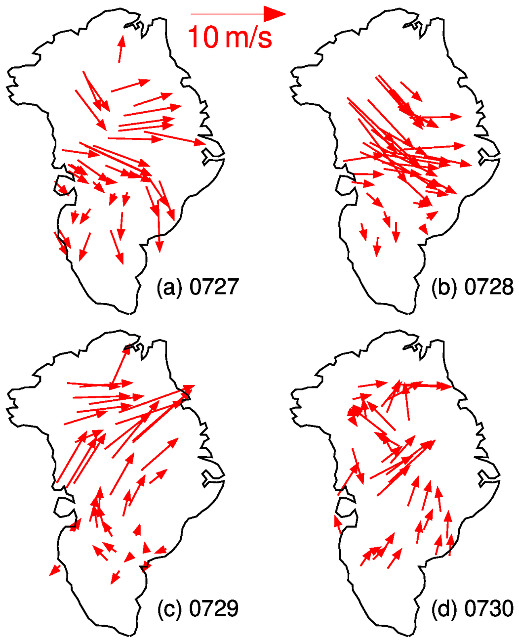
Figure 14Wind direction (referenced to the north) and wind speed (unit: m/s) over Greenland during 27–30 July 2017 (data from ECMWF).
The above analysis shows the promising quality of XBAER-derived SGS, SPS and SSA results. The XBAER-retrieved SGS, SPS and SSA can be used to understand the change in snow properties temporally. Even though the snow metamorphism depends on the environmental conditions, Aoki et al. (2000) and Saito et al. (2019) pointed out that a 4 d timescale is a reasonable time span to see the temporal change in snow properties. Figure 13 shows XBAER-derived SGS (upper panels), SPS (middle panels) and SSA (lower panels) over Greenland during 27–30 July 2017. Large variability for SGS, SPS and SSA can be seen during these 4 d, indicating the impacts of snow metamorphism on the snow properties. Figure 13 shows the snow melting process in both western and northeastern parts of Greenland, especially on 28 July. The strong melting in July over Greenland has also been reported by Lyapustin et al. (2009). The SPS over the southeastern part of Greenland becomes smaller during those 4 d. No snowfall was reported according to the relevant Polar Portal report (http://polarportal.dk/en/greenland/surface-conditions/, last access: 13 June 2021) during these 4 d; thus the smaller SGS may be caused by a local snow metamorphism process and/or due to the wind-blown fresh snow, transported from central Greenland to southeastern parts. However, possible cloud contamination over the northwest of Greenland may occur, leading to a very small SGS. The change in SGS is also consistent with the change in SPS. Please note that since the SGS and SPS are retrieved simultaneously, the selection of different SPSs leads to a different SGS; thus the change in SGS and SPS with respect to time may also be affected by the algorithm itself. In this section, we try to explain the change by the transport according to wind direction as presented in Fig. 14. Please note that other possible reasons (cloud contamination, algorithm issues, snow metamorphism process) can also be used to explain the geographic patterns. According to Fig. 14, the wind speed is over 6 m/s, which is strong enough to blow the surface ice crystal up. According to Fig. 13, SPSs over Greenland derived from the XBAER algorithm are mainly droxtals and solid bullet rosettes for the selected days. Solid bullet rosette and droxtal are typical ice crystal shapes for fresh snow and aged snow (Nakamura et al., 2001), respectively. The wind-blown fresh snow might be transported to the eastern part of Greenland, and fresh snow covers the original aged snow; thus a solid bullet rosette shape is retrieved. According to Fig. 8, droxtals and solid bullet rosettes retrieved by XBAER may link to faceted crystals and rounded grains in ICSSG, respectively. During the transport, faceted crystals turn into rounded grains. The change in SSA follows the change in SGS and SPS. The SSA over central Greenland is larger, while it is smaller in the coastline regions. This can be explained by the reduced SPMP impact on the snow properties due to the increase in elevation in central Greenland. Inversely proportional to SGS, the SSA reduces. The coverage of a large SSA over the eastern part of Greenland increases during these 4 d, indicating the “snowfall” feature due to transport. This wind-induced transport feature, similarly to fresh snowfall, changes both SGS and SPS. And this process is revealed by and superimposed on the SPMP during the temporal change in SSA retrieved from satellite observations (Carlsen et al., 2017).
SGS, SPS and SSA are three important parameters to describe snow properties. SGS, SPS and SSA all play important roles in the changes in snow albedo/reflectance and further impact the atmospheric and energy exchange processes. A better knowledge of SGS, SPS and SSA can provide more accurate information to describe the impact of snow on Arctic amplification processes. The information about SGS, SPS and SSA may also be used to explore new applications to understand atmospheric conditions (e.g., aerosol loading). Although some previous attempts (e.g., Lyapustin et al., 2009) show the capabilities of using passive remote sensing to derive SGS over a large scale, no publications have been found that derive SGS, SPS and SSA simultaneously. This is the first paper, to the best of our knowledge, attempting to retrieve SGS, SPS and SSA using passive remote sensing observations.
The new algorithm is designed within the framework of the XBAER algorithm. The XBAER algorithm has been applied to derive SGS, SPS and SSA using the newly launched SLSTR instrument on board the Sentinel-3 satellite. The cloud screening is performed with a synergistical technique using both OLCI and SLSTR measurements. The synergistical cloud screening in XBAER is easily implementable and effectively runnable on a global scale, with a high quality, which enables a cloud-contamination-minimized SGS, SPS and SSA retrieval using passive remote sensing.
Besides the cloud screening, another pre-process is the atmospheric correction. Aerosols have a non-ignorable impact on the retrieval of SGS, SPS and SSA, even over the Arctic regions, where aerosol loading is small (AOT at 0.55 µm is around 0.05) (Mei et al., 2020b). In the XBAER algorithm, the MERRA-simulated AOT at 0.55 µm, together with a weak-absorption aerosol type (Mei et al., 2020b), is used as the input for the atmospheric corrections.
The SGS, SPS and SSA retrieval algorithm is based on the publication by Yang et al. (2013), in which a database of optical properties for nine typical ice crystal shapes are provided. Previous publications show that this database can be used to retrieve ice crystal properties in both ice cloud and snow layers (e.g., Järvinen et al., 2018; Saito et al., 2019). The algorithm is a LUT-based approach, in which the minimization is achieved by the comparison between atmosphere-corrected TOA reflectance at 0.55 and 1.6 µm observed by SLSTR and a pre-calculated LUT under different geometries and snow properties. The retrieval is relatively time-consuming because the minimization has to be performed for each ice crystal shape and the optimal SGS and SPS are selected after the nine minimizations are performed. The SSA is then calculated using the retrieved SGS and SPS based on another pre-calculated LUT.
The comparison between XBAER-derived SGS, SPS and SSA shows good agreement with the SnowEx17 campaign measurements. The average absolute and relative difference between XBAER-derived SGS and SnowEx17-measured SGS is about 10 µm and 4 %, respectively. XBAER-derived SGS also shows good agreement with the MODIS SGS product. The XBAER-retrieved SPS reveals reasonable and explainable linkage with SnowEx17 measurements. The difference in XBAER-derived SSA and SnowEx17-measured SSA is 2.7 m2/kg. The retrieval results over Greenland reveal the general patterns of snow properties over Greenland, which are consistent with previous publications (Lyapustin et al., 2009). The change in SGS, SPS and SSA on a 4 d time span is also observed using XBAER-retrieved SGS, SPS and SSA. The comparison with aircraft measurements during the PAMARCMiP campaign held in March 2018 also indicates good agreement (R = 0.82 and R = 0.81 for SGS and SSA, respectively), XBAER-derived SGS and SSA reveal the variabilities in the aircraft track of the PAMARCMiP campaign. Intensive validation is performed using seven additional field-based measurements. XBAER-derived SGS and SSA show high correlation with field measurements, with correlation coefficients higher than 0.85. The RMSEs for SGS and SSA are less than 15 µm and 10 m2/kg, respectively. The validation of SPS reveals that the XBAER-derived aggregate SPS is likely to be matched with rounded grains while a single SPS in XBAER is possibly linked to faceted crystals in the ICSSG classification. This possible linkage, although inaccurate, will be helpful to understand the snow properties on a large scale.
Although the presented version of the XBAER retrieval algorithm shows promising results, we see at least four possibilities for improving its accuracy. Potential cloud contamination may still occur according to the analysis, exploiting the time-series technique, as described in Jafariserajehlou et al. (2019). Currently only a single-ice-crystal shape is used in the retrieval; the mixture of different ice crystal shapes, i.e., the snow grain habit mixture model (e.g., Saito et al., 2019), will be tested in further work. Another potential improvement may be linked to the use of polydisperse ice crystals (e.g., gamma distribution). The potential impacts of the vertical structure of SGS and SPS also need to be investigated in the future.
XBAER-derived SGS, SPS and SSA will be used to support the analysis of the MOSAiC expedition and other campaign-based measurements (Jäkel et al., 2021).
The data over the Antarctica site are provided by Ghislain Picard. The data over the Greenland site are provided by Hans Christian Steen-Larsen. The data over the Canada-Alex site are provided by Alexandre Langlois. The data over the Canada-Josh site are provided by Joshua King. The data over the China site are provided by Tao Che. The data over the Japan site are available at https://doi.org/10.1594/PANGAEA.909880 (Yamaguchi et al., 2019). The data over the Alps site are available at https://perscido.univ-grenoble-alpes.fr/datasets/DS330 (Dumont et al., 2013). The data over the SnowEx site are available at https://nsidc.org (https://doi.org/10.5067/G21LGCNLFSC, Webb et al., 2019; https://doi.org/10.5067/SNMM6NGGKWIT, Durand et al., 2020). The wind speed and wind direction data are from ECMWF. The PAMARCMiP 2018 data are available at https://doi.org/10.1594/PANGAEA.932527 (Jäkel et al., 2021).
LM and VR conceptualized the study, LM implemented the code and processed the data. LM, VR EJ, XC analyzed the data. LM prepared the manuscript with contribution from all co-authors. LM, VR, MV and JPB polished the whole manuscript.
The authors declare that they have no conflict of interest.
This research was funded by the Deutsche Forschungsgemeinschaft (DFG, German Research Foundation) – Project ID 268020496 – TRR 172. The comments by Alexandre Langlois, Ghislain Picard and the anonymous reviewer helped to improve the quality of the manuscript significantly. The authors highly appreciate the effort from Adam Povey (University of Oxford) to help to deal with the huge number of SLSTR L1 data. The authors would like to thank Knut von Salzen from Environment and Climate Change Canada for valuable discussion. We thank the support from Lisa Booker from the National Snow and Ice Data Center, Boulder, in understanding the SnowEx17 campaign data. We thank Alexander Kokhanovsky from Vitrociset, Darmstadt, Germany, and Jason E. Box from the Geological Survey of Denmark and Greenland (GEUS) for valuable discussion. We thank Salguero Jaime for providing the MODSCAG snow products. The MODIS snow product data are provided by MODSCAG team, and SLSTR–OLCI data are provided by ESA. The Zoom meeting and valuable discussion with Joshua King are highly appreciated.
This research has been supported by the Deutsche Forschungsgemeinschaft (grant no. 268020496 – TRR 172).
The article processing charges for this open-access publication were covered by the University of Bremen.
This paper was edited by Alexandre Langlois and reviewed by Ghislain Picard and one anonymous referee.
Aoki, T., Fukabori, M., Hachikubo, A., Tachibana, Y., and Nishio, F.: Effects of snow physical parameters on spectral albedo and bidirectional reflectance of snow surface, J. Geophys. Res., 105, 10219–10236, 2000.
Aoki, T., Hori, M., Motoyoshi, H., Tanikawa, T., Hachikubo, A., Sugiura, K., Yasunari, T., Storvold, R., Eide, H., Stamnes, K., Li, W., Nieke, J., Nakajima, Y., and Takahashi, F.: ADEOS-II/GLI snow/ice products – part II: Validation results using GLI and MODIS data, Remote Sens. Environ., 111, 274–290, https://doi.org/10.1016/j.rse.2007.02.035, 2007.
Avanzi, F., Johnson, R. C., Oroza, C. A., Hirashima, H., Maurer, T., and Yamaguchi, S.: Insights into preferentialflow snowpack runoffusing random forest, Water Resour. Res., 55, 10727–10746, 2019.
Barnett, T. P., Adam, J. C., and Lettenmaier, D. P.: Potential impacts of a warming climate on water availability in snow-dominated regions, Nature, 438, 303–309, 2005.
Beck, A., Henneberger, J., Fugal, J. P., David, R. O., Lacher, L., and Lohmann, U.: Impact of surface and near-surface processes on ice crystal concentrations measured at mountain-top research stations, Atmos. Chem. Phys., 18, 8909–8927, https://doi.org/10.5194/acp-18-8909-2018, 2018.
Bokhorst, S., Pedersen, S. H., Brucker, L., Anisimov, O., Bjerke, J. W., Brown, R. D., Ehrich, D., Essery, R. L. H., Heilig, A., Ingvander, S., Johansson, C., Johansson, M., Jónsdóttir, I. S., Inga, N., Luojus, K., Macelloni, G., Mariash, H., McLennan, D., Rosqvist, G. N., Sato, A., Savela, H., Schneebeli, M., Sokolov, A., Sokratov, S. A., Terzago, S., Vikhamar-Schuler, D., Williamson, S., Qiu, Y., and Callaghan, T. V.: Changing Arctic snow cover: A review of recent developments and assessment of future needs for observations, modelling, and impacts, Ambio, 45, 516–537, https://doi.org/10.1007/s13280-016-0770-0, 2016.
Brucker, L., Hiemstra, C., Marshall, H.-P., Elder, K., De Roo, R., Mousavi, M., Bliven, F., Peterson, W., Deems, J., Gadomski, P., Gelvin, A., Spaete, L., Barnhart, T., Brandt, T., Burkhart, J., Crawford, C., Dutta, T., Erikstrod, H., Glenn, N., Hale, K., Holben, B., Houser, P., Jennings, K., Kelly, R., Kraft, J., Langlois, A., McGrath, D., Merriman, C., Molotch, N., and Nolin, A.: A first overview of SnowEx ground-based remote sensing activities during the winter 2016–2017, in: 2017 IEEE International Geoscience and Remote Sensing Symposium (IGARSS), 1391–1394, https://doi.org/10.1109/IGARSS.2017.8127223, 2017.
Chandrasekhar, S.: Raditive Transfer, Oxford University Press, London, UK, 1950.
Carlsen, T., Birnbaum, G., Ehrlich, A., Freitag, J., Heygster, G., Istomina, L., Kipfstuhl, S., Orsi, A., Schäfer, M., and Wendisch, M.: Comparison of different methods to retrieve optical-equivalent snow grain size in central Antarctica, The Cryosphere, 11, 2727–2741, https://doi.org/10.5194/tc-11-2727-2017, 2017.
Chen, T., Pan, J., Chang, S., Xiong, C., Shi, J., Liu, M., Che, T., Wang, L., and Liu, H.: Validation of the SNTHERM Model Applied for Snow Depth, Grain Size, and Brightness Temperature Simulation at Meteorological Stations in China, Remote Sens., 12, 507, https://doi.org/10.3390/rs12030507, 2020.
Cohen, J. and Rind, D.: The Effect of Snow Cover on the Climate, J. Climate, 4, 689–706, https://doi.org/10.1175/1520-0442(1991)004<0689:TEOSCO>2.0.CO;2, 1991.
Colbeck, S. C.: Thermodynamics of snow metamorphism due to variations in curvature, J. Glaciol., 26, 291–301, https://doi.org/10.3189/S0022143000010832, 1980.
Colbeck, S. C.: Theory of metamorphism of dry snow, J. Geophys. Res., 88, 5475–5482, 1983.
Cole, B. H., Yang, P., Baum, B. A., Riedi, J., and C.-Labonnote, L.: Ice particle habit and surface roughness derived from PARASOL polarization measurements, Atmos. Chem. Phys., 14, 3739–3750, https://doi.org/10.5194/acp-14-3739-2014, 2014.
Comola, F., Kok, J. F., Gaume, J., Paterna, E., and Lehning, M.: Fragmentation of wind-blown snow crystals, Geophys. Res. Lett., 44, 4195–4203, https://doi.org/10.1002/2017GL073039, 2017GL073039, 2017.
Dang, C., Fu, Q., and Warren, S. G.: Effect of snow grain shape on snow albedo, J. Atmos. Sci., 73, 3573–3583, https://doi.org/10.1175/JAS-D-15-0276.1, 2016.
Dumont, M., Brissaud, O., Picard, G., Schmitt, B., Gallet, J.-C., and Arnaud, Y.: High-accuracy measurements of snow Bidirectional Reflectance Distribution Function at visible and NIR wavelengths – comparison with modelling results, Atmos. Chem. Phys., 10, 2507–2520, https://doi.org/10.5194/acp-10-2507-2010, 2010.
Dumont, M., Tuzet, F., Revuelto, J., Arnaud, L., Dumont, M., Picard, G., Lamare, M., Voisin, D., Nabat, P., Lafaysse, M., and Larue, F.: Field campaign at Col du Lautaret 2016–2018 (2058 m a.s.l., French Alps), Snow surface properties and albedo measurements at Col du Lautaret, available at: https://perscido.univ-grenoble-alpes.fr/datasets/DS330, last access: 13 June 2013.
Durand, M., Vuyovich, C. M., Lemmetyinen, J., Vargel, C., Hale, K., and Yang, K.: SnowEx20 Laser Snow Microstructure Specific Surface Area Data, Version 1, Boulder, Colorado USA, NASA National Snow and Ice Data Center Distributed Active Archive Center, https://doi.org/10.5067/SNMM6NGGKWIT, 2020.
Egerer, U., Gottschalk, M., Siebert, H., Ehrlich, A., and Wendisch, M.: The new BELUGA setup for collocated turbulence and radiation measurements using a tethered balloon: first applications in the cloudy Arctic boundary layer, Atmos. Meas. Tech., 12, 4019–4038, https://doi.org/10.5194/amt-12-4019-2019, 2019.
Elder, K., Brucker, L., Hiemstra, C., and Marshall, H.: SnowEx17 Community Snow Pit Measurements, Version 1 [Indicate subset used], NASA National Snow and Ice Data Center Distributed Active Archive Center, Boulder, Colorado, USA, https://doi.org/10.5067/Q0310G1XULZS, 2018.
Fang, X. and Pomeroy, J. W.: Modelling blowing snow redistribution to Prairie wetlands, Hydrol. Process., 23, 2557–2569, https://doi.org/10.1002/hyp.7348, 2009.
Fierz, C., Armstrong, R. L., Durand, Y., Etchevers, P., Greene, E., McClung, D. D., Nishimura, K., Satyawali, P. K., and Sokratov, S. A.: The International Classification for seasonal snow on the ground, IHP-VII Technical Documents in Hydrology No. 83, IACS Conribution No. 1, UNESCO-IHP, Paris, France, 2009.
Flanner, M. G. and Zender, C. S.: Linking snowpack microphysics and albedo evolution, J. Geophys. Res.-Atmos., 111, D12208, https://doi.org/10.1029/2005JD006834, 2006.
Flanner, M. G., Shell, K., Barlage, M., Perovich, D. K., and Tschudi, M. A.: Radiative forcing and albedo feedback from the Northern Hemisphere cryosphere between 1979 and 2008, Nat. Geosci., 4, 151–155, https://doi.org/10.1038/ngeo1062, 2011.
Gallet, J.-C., Domine, F., Zender, C. S., and Picard, G.: Measurement of the specific surface area of snow using infrared reflectance in an integrating sphere at 1310 and 1550 nm, The Cryosphere, 3, 167–182, https://doi.org/10.5194/tc-3-167-2009, 2009.
Gastineau, G., García-Serrano, J., and Frankignoul, C.: The Influence of Autumnal Eurasian Snow Cover on Climate and Its Link with Arctic Sea Ice Cover, J. Climate, 30, 7599–7619, https://doi.org/10.1175/JCLI-D-16-0623.1, 2017.
Gordon, M. and Taylor, P. A.: The Electric Field During Blowing Snow Events, Bound-Lay. Meteorol., 130, 97–115, 2009.
Groot Zwaaftink, C. D., Löwe, H., Mott, R., Bavay, M., and Lehning, M.: Drifting snow sublimation: A high-resolution 3-D model with temperature and moisture feedbacks, J. Geophys. Res.-Atmos., 116, D16107, https://doi.org/10.1029/2011jd015754, 2011.
Hansen, J., Lacis, A., Rind, D., Russell, G., Stone, P., Fung, I., Ruedy, R., and Lerner, J.: Climate Sensitivity: Analysis of Feedback Mechanisms, in: Climate Processes and Climate Sensitivity, edited by: Hansen, J. E. and Takahashi, T., AGU Geophys. Monogr. Ser. 29, National Academies of Sciences, Engineering, and Medicine, Washington, D.C., USA, 130–163, 1984.
Henderson, G. R., Peings, Y., Furtado, J. C., and Kushner, P. J.: Snow-atmosphere coupling in the Northern Hemisphere, Nat. Clim. Change, 8, 954–963, https://doi.org/10.1038/s41558-018-0295-6, 2018.
Hori, M., Aoki, T., Stamnes, K., and Li, W.: ADEOS-II/GLI snow/ice products – part III: retrieved results, Remote Sens. Environ., 111, 291–336, https://doi.org/10.1016/j.rse.2007.01.025, 2007.
Hyvarinen, T. and Lammasniemi, J.: Infrared measurement of free-water content and grain size of snow, Opt. Eng., 26, 342–348, 1987.
Ishimoto, H., Adachi, S., Yamaguchi, S., Tanikawa, T., Aoki, T., and Masuda, K.: Snow particles extracted from X-ray computed microtomography imagery and their single-scattering properties, J. Quant. Spectrosc. Ra., 209, 113–128, https://doi.org/10.1016/j.jqsrt.2018.01.021, 2018.
Istomina, L. G., von Hoyningen-Huene, W., Kokhanovsky, A. A., and Burrows, J. P.: The detection of cloud-free snow-covered areas using AATSR measurements, Atmos. Meas. Tech., 3, 1005–1017, https://doi.org/10.5194/amt-3-1005-2010, 2010.
Jäkel, E., Mey, B., Levy, R., Gu, X., Yu, T., Li, Z., Althausen, D., Heese, B., and Wendisch, M.: Adaption of the MODIS aerosol retrieval algorithm using airborne spectral surface reflectance measurements over urban areas: a case study, Atmos. Meas. Tech., 8, 5237–5249, https://doi.org/10.5194/amt-8-5237-2015, 2015.
Jäkel, E., Ehrlich, A., Herber, A., and Carlsen, T.: Optical-equivalent snow grain size retrieved from airborne spectral surface albedo measurements during PAMARCMiP 2018, PANGAEA, https://doi.org/10.1594/PANGAEA.932527, 2021.
Järvinen, E., Jourdan, O., Neubauer, D., Yao, B., Liu, C., Andreae, M. O., Lohmann, U., Wendisch, M., McFarquhar, G. M., Leisner, T., and Schnaiter, M.: Additional global climate cooling by clouds due to ice crystal complexity, Atmos. Chem. Phys., 18, 15767–15781, https://doi.org/10.5194/acp-18-15767-2018, 2018.
Jeoung, H., Liu, G., Kim, K., Lee, G., and Seo, E.-K.: Microphysical properties of three types of snow clouds: implication for satellite snowfall retrievals, Atmos. Chem. Phys., 20, 14491–14507, https://doi.org/10.5194/acp-20-14491-2020, 2020.
Jin, Z., Charlock, T. P., Yang, P., Xie, Y., and Miller, W.: Snow optical properties for different particle shapes with application to snow grain size retrieval and MODIS/CERES radiance comparison over Antarctica, Remote Sens. Environ., 112, 3563–3581, https://doi.org/10.1016/j.rse.2008.04.011, 2008.
Kaufman, Y. J., Tanre, D., Remer, L. A., Vermote, E. F., Chu, A., and Holben, B. N.: Operational remote sensing of tropospheric aerosol over land from EOS moderate resolution imaging spectroradiometer, J. Geophys. Res.-Atmos., 102, 17051–17067, https://doi.org/10.1029/96JD03988, 1997.
Key, J., Mahoney, R., Liu, Y., Romanov, P., Tschudi, M., Appel, I., Maslanik, J., Baldwin, D., Wang, X., and Meade, P.: Snow and ice products from Suomi NPP VIIRS, J. Geophys. Res.-Atmos., 118, 12816–12830, 2013.
Kikuchi, K., Kameda, T., Higuchi, K., and Yamashita, A.: A global classification of snow crystals, ice crystals, and solid precipitation based on observations from middle latitudes to polar regions, Atmos. Res., 132–133, 460–472, 2013.
Kim, E., Gatebe, C., Hall, D., Newlin, J., Misakonis, A., Elder, K., Marshall, H., Hiemstra, C., Brucker, L., De Marco, E., Crawford, C., Kang, D. H., and Entin, J.: NASA's SnowEx campaign: Observing seasonal snow in a forested environment, in: 2017 IEEE International Geoscience and Remote Sensing Symposium (IGARSS), https://doi.org/10.1109/IGARSS.2017.8127222, 2017.
King, J., Derksen, C., Toose, P., Montpetit, B., and Siqueira, P.: TVCSnow: Seasonal Ku-band (13.25 GHz) SAR measurements in a snow-covered tundra basin, in: 76th Annual Eastern Snow Conference, Vermont, USA, June 2019.
King, M. D., Platnick, S., Menzel, W. P., Ackerman, S. A., and Hubanks, P. A.: Spatial and temporal distribution of clouds observed by MODIS onboard the Terra and Aqua satellites, IEEE T. Geosci. Remote, 51, 3826–3852, 2013.
Klein, A. G. and Stroeve, J.: Development and validation of a snow albedo algorithm for the MODIS instrument, Ann. Glaciol., 34, 45–52, 2002.
Kokhanovsky, A., Lamare, M., Di Mauro, B., Picard, G., Arnaud, L., Dumont, M., Tuzet, F., Brockmann, C., and Box, J. E.: On the reflectance spectroscopy of snow, The Cryosphere, 12, 2371–2382, https://doi.org/10.5194/tc-12-2371-2018, 2018.
Kokhanovsky, A., Lamare, M., Danne, O., Brockmann, C., Dumont, M., Picard, G., Arnaud, L., Favier, V., Jourdain, B., Le Meur, E., Di Mauro, B., Aoki, T., Niwano, M., Rozanov, V., Korkin, S., Kipfstuhl, S., Freitag, J., Hoerhold, M., Zuhr, A., Vladimirova, D., Faber, A.-K., Steen-Larsen, H. C., Wahl, S., Andersen, J. K., Vandecrux, B., van As, D., Mankoff, K. D., Kern, M., Zege, E., and Box, J. E.: Retrieval of Snow Properties from the Sentinel-3 Ocean and Land Colour Instrument, Remote Sens., 11, 2280, https://doi.org/10.3390/rs11192280, 2019.
Kokhanovsky, A. A. and Zege, E. P.: Scattering optics of snow, Appl. Optics, 43, 1589–1602, 2004.
Koren, I., Remer, L., Kaufman, Y. J., Rudich, Y., and Martins, J.: On the twilight zone between clouds and aerosols, Geophys. Res. Lett., 34, L08805, https://doi.org/10.1029/2007GL029253, 2007.
LaChapelle, E. R.: Field Guide to Snow Crystals, University of Washington Press, Univ. of Washington Pr., 112 pp., 1969.
Lawson, P., Baker, B., Zmarzly, P., O'Connor, D., Mo, Q., Gayet, J.-F., and Shcherbakov, V.: Microphysical and optical properties of ice crystals at South Pole Station, J. Appl. Meteorol. Clim., 45, 1505–1524, https://doi.org/10.1175/JAM2421.1, 2006.
Lemke, P., Ren, J., Alley, R. B., Allison, I., Carrasco, J., Flato, G., Fujii, Y., Kaser, G., Mote, P., Thomas, R. H., and Zhang, T.: Observations: Changes in Snow, Ice and Frozen Ground, in: Climate Change 2007: The Physical Science Basis, Contribution of Working Group I to the Fourth Assessment Report of the Intergovernmental Panel on Climate Change, edited by: Solomon, S., Qin, D., Manning, M., Chen, Z., Marquis, M., Averyt, K. B., Tignor, M., and Miller, H. L., Cambridge University Press, Cambridge, UK, New York, USA, 2007.
Leroux, C. and Fily, M.: Modeling the effect of sastrugi on snow reflectance, J. Geophys. Res., 103, 25779–25788, 1998.
Li, W., Stamnes, K., Chen, B., and Xiong, X.: Snow grain size retrieved from near-infrared radiances at multiple wavelengths, Geophys. Res. Lett., 28, 1699–1702, https://doi.org/10.1029/2000GL011641, 2001.
Libois, Q., Picard, G., Arnaud, L., Morin, S., and Brun, E.: Modeling the impact of snow drift on the decameter-scale variability of snow properties on the Antarctic Plateau, J. Geophys. Res., 119, 1662–1681, 2014.
Liston, G. E. and Hiemstra, C. A.: The Changing Cryosphere: Pan-Arctic Snow Trends (1979–2009), J. Climate, 24, 5691–5712, https://doi.org/10.1175/JCLI-D-11-00081.1, 2011.
Liu, X. and Yanai, M.: Influence of Eurasian spring snow cover on Asian summer rainfall, Int. J. Climatol., 22, 1075–1089, https://doi.org/10.1002/joc.784, 2002.
Lyapustin, A., Tedesco, M., Wang, Y. J., Aoki, T., Hori, M., and Kokhanovsky, A.: Retrieval of snow grain size over Greenland from MODIS, Remote Sens. Environ., 113, 1976–1987, 2009.
Lyapustin, A., Wang, Y., Xiong, X., Meister, G., Platnick, S., Levy, R., Franz, B., Korkin, S., Hilker, T., Tucker, J., Hall, F., Sellers, P., Wu, A., and Angal, A.: Scientific impact of MODIS C5 calibration degradation and C6+ improvements, Atmos. Meas. Tech., 7, 4353–4365, https://doi.org/10.5194/amt-7-4353-2014, 2014.
Lyapustin, A. I.: Atmospheric and geometrical effects on land surface albedo, J. Geophys. Res.-Atmos., 104, 4127–4143, https://doi.org/10.1029/1998jd200064, 1999.
Macke, A., Mueller, J., and Raschke, E.: Single scattering properties of atmospheric ice crystals, J. Atmos. Sci., 53, 2813–2825, 1996.
Mary, A., Dumont, M., Dedieu, J.-P., Durand, Y., Sirguey, P., Milhem, H., Mestre, O., Negi, H. S., Kokhanovsky, A. A., Lafaysse, M., and Morin, S.: Intercomparison of retrieval algorithms for the specific surface area of snow from near-infrared satellite data in mountainous terrain, and comparison with the output of a semi-distributed snowpack model, The Cryosphere, 7, 741–761, https://doi.org/10.5194/tc-7-741-2013, 2013.
McFarlane, S. A., Marchand, R. T., and Ackerman, T. P.: Retrieval of cloud phase and crystal habit from Multiangle Imaging Spectroradiometer (MISR) and Moderate Resolution Imaging Spectroradiometer (MODIS) data, J. Geophys. Res.-Atmos., 110, D14201, https://doi.org/10.1029/2004JD004831, 2005.
Mei, L., Rozanov, V., Vountas, M., Burrows, J. P., Levy, R. C., and Lotz, W.: Retrieval of aerosol optical properties using MERIS observations: Algorithm and some first results, Remote Sens. Environ., 197, 125–140, https://doi.org/10.1016/j.rse.2016.11.015, 2017a.
Mei, L., Rozanov, V., Vountas, M., Burrows, J., Levy, R., and Lotz, W.: A Cloud masking algorithm for the XBAER aerosol retrieval using MERIS data, Remote Sens. Environ., 197, 141–160, https://doi.org/10.1016/j.rse.2016.11.016, 2017b.
Mei, L., Rozanov, V., Vountas, M., and Burrows, J. P.: The retrieval of ice cloud parameters from multi-spectral satellite observations of reflectance using a modified XBAER algorithm, Remote Sens. Environ., 215, 128–144, 2018.
Mei, L., Vandenbussche, S., Rozanov, V., Proestakis, E., Amiridis, V., Callewaert, S., Vountas, M., and Burrows, J. P.: On the retrieval of aerosol optical depth over cryosphere using passive remote sensing, Remote Sens. Environ., 241, 111731, https://doi.org/10.1016/j.rse.2020.111731, 2020a.
Mei, L., Rozanov, V., Ritter, C., Heinold, B., Jiao, Z. T., Vountas, M., and Burrows, J. P.: Retrieval of aerosol optical thickness in the Arctic snow-covered regions using passive remote sensing: impact of aerosol typing and surface reflection model, IEEE T. Geosci. Remote, 58, 5117–5131, https://doi.org/10.1109/TGRS.2020.2972339, 2020b.
Mei, L., Rozanov, V., and Burrows, J. P.: A fast and accurate radiative transfer model for aerosol remote sensing, J. Quant. Spectrosc. Ra., 256, 107270, https://doi.org/10.1016/j.jqsrt.2020.107270, 2020c.
Mei, L., Rozanov, V., Pohl, C., Vountas, M., and Burrows, J. P.: The retrieval of snow properties from SLSTR Sentinel-3 – Part 1: Method description and sensitivity study, The Cryosphere, 15, 2757–2780, https://doi.org/10.5194/tc-15-2757-2021, 2021a.
Mei, L., Rozanov, V., Jiao, Z., and Burrows, J. P.: A new snow bidirectional reflectance distribution function model in spectral regions from UV to SWIR, in preparation, 2021b.
Montpetit, B., Royer, A., Langlois, A., Cliché, P., Roy, A., Champollion, N., Picard, G., Domine, F., and Obbard, R.: Instruments and methods new shortwave infrared albedo measurements for snow specific surface area retrieval, J. Glaciol., 58, 941–952, 2012.
Nakamura, T., Abe, O., Hasegawa, T., Tamura, R., and Ohta, T.: Spectral reflectance of snow with a known particle-size distribution in successive metamorphism, Cold Reg. Sci. Technol., 32, 13–26, https://doi.org/10.1016/S0165-232X(01)00019-2, 2001.
Nakaya, U. and Sekido, Y.: General Classification of Snow Crystals and their Frequency of Occurrence, Journal of the Faculty of Science Ser. 2-Physics, Hokkaido Imperial University, Sapporo, Hokkaidō, Japan, 243–264, 1938.
Nakoudi, K., Ritter, C., Böckmann, C., Kunkel, D., Eppers, O., Rozanov, V., Mei, L., Pefanis, V., Jäkel, E., Herber, A., Maturilli, M., and Neuber, R.: Does the Intra-Arctic Modification of Long-Range Transported Aerosol Affect the Local Radiative Budget? (A Case Study), Remote Sens., 12, 2112, https://doi.org/10.3390/rs12132112, 2020.
Negi, H. S. and Kokhanovsky, A.: Retrieval of snow albedo and grain size using reflectance measurements in Himalayan basin, The Cryosphere, 5, 203–217, https://doi.org/10.5194/tc-5-203-2011, 2011.
Painter, T. H., Dozier, J., Roberts, D. A., Davis, R. E., and Greene, R. O.: Retrieval of subpixel snow-covered area and grain size from imaging spectrometer data, Remote Sens. Environ., 85, 64–77, 2003.
Painter, T. H., Rittger, K., McKenzie, C., Slaughter, P., Davis, R. E., and Dozier, J.: Retrieval of subpixel snow covered areas, grain size, and albedo from MODIS, Remote Sens. Environ., 113, 868–879, 2009.
Picard, G., Libois, Q., Arnaud, L., Verin, G., and Dumont, M.: Development and calibration of an automatic spectral albedometer to estimate near-surface snow SSA time series, The Cryosphere, 10, 1297–1316, https://doi.org/10.5194/tc-10-1297-2016, 2016.
Pirazzini, R., Räisänen, P., Vihma, T., Johansson, M., and Tastula, E.-M.: Measurements and modelling of snow particle size and shortwave infrared albedo over a melting Antarctic ice sheet, The Cryosphere, 9, 2357–2381, https://doi.org/10.5194/tc-9-2357-2015, 2015.
Platnick, S., Meyer, K. G., King, M. D., Wind, G., Amarasinghe, N., Marchant, B., Arnold, G. T., Zhang, Z. B., Hubanks, P., Holz, R., Yang, P., Lidgway, W., and Riedi, J.: The MODIS cloud optical and microphysical products: Collection 6 updates and examples from Terra and Aqua, IEEE T. Geosci. Remote, 55, 502–525, 2017.
Pohl, C., Rozanov, V. V., Mei, L., Burrows, J. P., Heygster, G., and Spreen, G.: Implementation of an ice crystal single-scattering property database in the radiative transfer model SCIATRAN, J. Quant. Spectrosc. Ra., 253, 107118, https://doi.org/10.1016/j.jqsrt.2020.107118, 2020.
Popp, T., de Leeuw, G., Bingen, C., Bruhl, C., Capelle, V., Chedin, A., Clarisse, L., Dubovik, O., Grainger, R., Griesfeller, J., Heckel, A., Kinne, S., Kluser, L., Kosmale, M., Kolmonen, P., Lelli, L., Litvinov, P., Mei, L., North, P., Pinnock, S., Povey, A., Robert, C., Schulz, M., Sogacheva, L., Stebel, K., Stein Zweers, D., Thomas, G., Tilstra, L. G., Vandenbussche, S., Veefkind, P., Vountas, M., and Xue, Y.: Development, Production and Evaluation of Aerosol Climate Data Records from European Satellite Observations (Aerosol_cci), Remote Sens., 8, 421, https://doi.org/10.3390/rs8050421, 2016.
Räisänen, P., Makkonen, R., Kirkevåg, A., and Debernard, J. B.: Effects of snow grain shape on climate simulations: sensitivity tests with the Norwegian Earth System Model, The Cryosphere, 11, 2919–2942, https://doi.org/10.5194/tc-11-2919-2017, 2017.
Rittger, K., Painter, T. H., and Dozier, J.: Assessment of methods for mapping snow cover from MODIS, Adv. Water Resour., 51, 367–380, https://doi.org/10.1016/j.advwatres.2012.03.002, 2013.
Rozanov, V. V., Rozanov, A. V., Kokhanovsky, A. A., and Burrows, J. P.: Radiative transfer through terrestrial atmosphere and ocean: Software package SCIATRAN, J. Quant. Spectrosc. Ra., 133, 13–71, 2014.
Rutter, N., Pan, J., Durand, M., King, J., Derksen, C., and Larue, F.: SnowEx17 Laser Snow Microstructure Specific Surface Area Data, Version 1 [Indicate subset used], NASA National Snow and Ice Data Center Distributed Active Archive Center, Boulder, Colorado, USA, https://doi.org/10.5067/H9C1UVWN1UK3, 2018.
Ryan, J. C., Smith, L. C., van As, D., Cooley, S. W., Cooper, M. G., Pitcher, L. H., and Hubbard, A.: Greenland Ice Sheet surface melt amplified by snowline migration and bare ice exposure, Science Advances, 5, eaav3738, https://doi.org/10.1126/sciadv.aav3738, 2019.
Saito, M., Yang, P., Loeb, N. G., and Kato, S.: A novel parameterization of snow albedo based on a two-layer snow model with a mixture of grain habits, J. Atmos. Sci., 76, 1419–1436, 2019.
Sarangi, C., Qian, Y., Rittger, K., Bormann, K. J., Liu, Y., Wang, H., Wan, H., Lin, G., and Painter, T. H.: Impact of light-absorbing particles on snow albedo darkening and associated radiative forcing over high-mountain Asia: high-resolution WRF-Chem modeling and new satellite observations, Atmos. Chem. Phys., 19, 7105–7128, https://doi.org/10.5194/acp-19-7105-2019, 2019.
Sokratov, S. and Kazakov, N.: Dry snow metamorphism expressed by crystal shape, Ann. Glaciol., 58, 51–56, 2012.
Stamnes, K., Li, W., Eide, H., Aoki, T., Hori, M., and Storvold, R.: ADEOSII/GLI snow/ice products – part I: Scientific basis, Remote Sens. Environ., 111, 258–273, https://doi.org/10.1016/j.rse.2007.03.023, 2007.
Tanikawa, T., Kuchiki, K., Aoki, T., Ishimoto, H., Hachikubo, A., Niwano, M., Hosaka, M., Matoba, S., Kodama, Y., Iwata, Y., and Stamnes, K.: Effects of snow grain shape and mixing state of snow impurity on retrieval of snow physical parameters from ground-based optical instrument, J. Geophys. Res.-Atmos., 125, e2019JD031858, https://doi.org/10.1029/2019JD031858, 2020.
Thackeray, C. W. and Fletcher, C. G.: Snow albedo feedback Current knowledge, importance, outstanding issues and future directions, Prog. Phys. Geog., 40, 392–408, https://doi.org/10.1177/0309133315620999, 2016.
Tuzet, F., Dumont, M., Picard, G., Lamare, M., Voisin, D., Nabat, P., Lafaysse, M., Larue, F., Revuelto, J., and Arnaud, L.: Quantification of the radiative impact of light-absorbing particles during two contrasted snow seasons at Col du Lautaret (2058 m a.s.l., French Alps), The Cryosphere, 14, 4553–4579, https://doi.org/10.5194/tc-14-4553-2020, 2020.
Webb, R., McGrath, D., Hale, K., and Molotch N. P.: SnowEx17 Ground Penetrating Radar, Version 2, Boulder, Colorado USA. NASA National Snow and Ice Data Center Distributed Active Archive Center, https://doi.org/10.5067/G21LGCNLFSC5, 2019.
Wendisch, M., Muller, D., Schell, D., and Heintzenberg, J.: An air-borne spectral albedometer with active horizontal stabilization, J. Atmos. Ocean. Tech., 18, 1856–1866, 2001.
Wendisch, M., Pilewskie, P., Jakel, E., Schmidt, S., Pommier, J., Howard, S., Jonsson, H. H., Guan, H., Schroder, M., and Mayer, B.: Airborne measurements of areal spectral surface albedo over different sea and land surfaces, J. Geophys. Res.-Atmos., 109, D08203, https://doi.org/10.1029/2003JD004392, 2004.
Wiebe, H., Heygster, G., Zege, E., Aoki, T., and Hori, M.: Snow grain size retrieval SGSP from optical satellite data: Validation with ground measurements and detection of snow fall events, Remote Sens. Environ., 128, 11–20, https://doi.org/10.1016/j.rse.2012.09.007, 2013.
Xiong, C. and Shi, J.: Snow specific surface area remote sensing retrieval using a microstructure based reflectance model, Remote Sens. Environ., 204, 838–849, https://doi.org/10.1016/j.rse.2017.09.017, 2018.
Yamaguchi, S., Hiroyuki, H., and Avanzi, F.: Daily summary of weather, snow, and preferential-flow conditions at the Snow and Ice Research Center, Nagaoka (Japan) – snow seasons 2006 through 2018, PANGAEA, https://doi.org/10.1594/PANGAEA.909880, 2019.
Yang, P., Bi, L., Baum, B. A., Liou, K.-N., Kattawar, G. W., Mishchenko, M. I., and Cole, B.: Spectrally consistent scattering, absorption, and polarization properties of atmospheric ice crystals at wavelengths from 0.2 to 100 µm, J. Atmos. Sci., 70, 330–347, 2013.
Zege, E. P., Kokhanovsky, A. A., Katsev, I. L., Polonsky, I. N., and Prikhach, A. S.: The retrieval of the effective radius of snow grains and control of snow pollution with GLI data, in: Proceedings of Conference on Light Scattering by Nonspherical Particles: Theory, Measurements, and Applications, edited by: Hovenier, M. I., NASA Goddard Institute for Space Studies, New York, USA, 29 September–1 October 1998, 288–290, 1998.
Zege, E. P., Katsev, I. L., Malinka, A. V., Prikhach, A. S., Heygster, G., and Wiebe, H.: Algorithm for retrieval of the effective snow grain size and pollution amount from satellite measurements, Remote Sens. Environ., 115, 2674–2685, 2011.
Zhang, T., Wang, T., Krinner, G., Wang, X., Gasser, T., Peng, S., Piao, S., and Yao, T.: The weakening relationship between Eurasian spring snow cover and Indian summer monsoon rainfall, Science Advances, 5, eaau8932, https://doi.org/10.1126/sciadv.aau8932, 2019.
Zhao, S., Jiang, T., and Wang, Z.: Snow grain-size estimation using Hyperion imagery in a typical area of the Heihe river basin, China, Remote Sens.-Basel, 5, 238–253, 2013.