the Creative Commons Attribution 4.0 License.
the Creative Commons Attribution 4.0 License.
 | 18 Jun 2021
The retrieval of snow properties from SLSTR Sentinel-3 – Part 1: Method description and sensitivity study
Linlu Mei
Vladimir Rozanov
Christine Pohl
Marco Vountas
John P. Burrows
The eXtensible Bremen Aerosol/cloud and surfacE parameters Retrieval (XBAER) algorithm has been designed for the top-of-atmosphere reflectance measured by the Sea and Land Surface Temperature Radiometer (SLSTR) instrument on board Sentinel-3 to derive snow properties: snow grain size (SGS), snow particle shape (SPS) and specific surface area (SSA) under cloud-free conditions. This is the first part of the paper, to describe the retrieval method and the sensitivity study. Nine pre-defined SPSs (aggregate of 8 columns, droxtal, hollow bullet rosette, hollow column, plate, aggregate of 5 plates, aggregate of 10 plates, solid bullet rosette, column) are used to describe the snow optical properties. The optimal SGS and SPS are estimated iteratively utilizing a look-up-table (LUT) approach. The SSA is then calculated using another pre-calculated LUT for the retrieved SGS and SPS. The optical properties (e.g., phase function) of the ice crystals can reproduce the wavelength-dependent and angular-dependent snow reflectance features, compared to laboratory measurements. A comprehensive study to understand the impact of aerosols, SPS, ice crystal surface roughness, cloud contamination, instrument spectral response function, the snow habit mixture model and snow vertical inhomogeneity in the retrieval accuracy of snow properties has been performed based on SCIATRAN radiative transfer simulations. The main findings are (1) snow angular and spectral reflectance features can be described by the predefined ice crystal properties only when both SGS and SPS can be optimally and iteratively obtained; (2) the impact of ice crystal surface roughness on the retrieval results is minor; (3) SGS and SSA show an inverse linear relationship; (4) the retrieval of SSA assuming a non-convex particle shape, compared to a convex particle shape (e.g., sphere), shows larger retrieval results; (5) aerosol/cloud contamination due to unperfected atmospheric correction and cloud screening introduces underestimation of SGS, “inaccurate” SPS and overestimation of SSA; (6) the impact of the instrument spectral response function introduces an overestimation into retrieved SGS, introduces an underestimation into retrieved SSA and has no impact on retrieved SPS; and (7) the investigation, by taking an ice crystal particle size distribution and habit mixture into account, reveals that XBAER-retrieved SGS agrees better with the mean size, rather than with the mode size, for a given particle size distribution.
- Article
(6516 KB) - Full-text XML
- Companion paper
- BibTeX
- EndNote


Snow properties such as snow albedo, snow grain size (SGS), snow particle shape (SPS), specific surface area (SSA) and snow purity (Warren and Wiscombe, 1980; Painter et al., 2003; Hansen and Nazarenko, 2004; Taillandier et al., 2007; Gallet et al., 2009; Battaglia et al., 2010; Gardner and Sharp, 2010; Domine et al., 2011; Liu et al., 2012; Qu et al., 2015; Baker, 2019; Pohl et al., 2020a) show large variabilities temporally and spatially (Kukla et al., 1986). They play important roles in the global radiation budget, which is critical to some well-known phenomena such as Arctic amplification (Serreze and Francis, 2006; Domine et al., 2019). Satellites offer an effective way to understand the surface–atmosphere processes and corresponding feedback mechanisms on the regional, continental and/or global scales (Konig et al., 2001; Pope et al., 2014). Satellite-derived snow products (e.g., SGS, SPS and SSA) are particularly important for short-term hydrological, meteorological and climatological modeling (Livneh et al., 2009). A high-quality snow property data product can also be applied to derive aerosol optical thickness (AOT) over the cryosphere (Mei et al., 2020a). High-quality satellite-derived snow products and their by-products are also important for the creation of long-term climate data records (SSMC, 2014), which enable better investigation and interpretation concerning global climate change (Konig et al., 2001). However, both the definition and the corresponding data accuracy of SGS are poor (Langlois et al., 2020), and there is no existing SPS satellite product. The lack of good information on SGS and SPS leads to a low quality of SSA (Gallet et al., 2009). The accuracy of SGS, SPS and SSA limits the model performance for the prediction of snow properties related to climate change issues. Lack of information on SGS and SPS also restricts the accuracy of snow bidirectional reflectance estimation, which further limits the retrieval possibilities of aerosol and cloud properties above snow (Mei et al., 2020a, b).
A comprehensive overview of remote sensing of SGS, SPS and SSA can be found in many previous publications (e.g., Li et al., 2001; Stamnes et al., 2007; Koren, 2009; Lyapustin et al., 2009; Dietz et al., 2012; Wiebe et al., 2013; Frei et al., 2012; Mary et al., 2013; Kokhanovsky, et al., 2019; Xiong and Shi, 2018). The variation in SGS leads to the large variability in top-of-atmosphere (TOA) reflectance in near-infrared (NIR)/shortwave infrared (SWIR) spectral ranges, and SPS shows a strong impact on TOA reflectance in visible channels (Warren and Wiscombe, 1980). Different retrieval algorithms have been developed for different instruments. For instance, the MODIS Snow-Covered Area and Grain size (MODSCAG) retrieval algorithm and Multi-Angle Implementation of Atmospheric Correction (MAIAC) algorithm have been used to derive SGS using MODIS and VIIRS instruments (Painter et al., 2003, 2009; Lyapustin et al., 2009).
Snow particle shape is another important parameter which affects the estimation of snow properties, such as albedo (Räisänen et al., 2017; Flanner and Zender, 2006), because ice crystals with different shapes have different optical properties (Jin et al., 2008; Yang et al., 2013). The absorption and extinction cross sections of an ice crystal can be described as a function of size, shape, and the refractive index at a given wavelength (van de Hulst, 1981; Mischenko et al., 2002, and references therein). Natural snow consists of grains, depending on temperature, humidity and meteorological conditions, which have numerous different shapes (Nakaya, 1954). SPSs have been classified into different categories; the classification has been increased from 21 (Nakaya and Sekido, 1938) to 121 (Kikuchi et al., 2013) categories. Although a spherical-shape assumption is typically used for field measurements (Flanner and Zender, 2006; Donahue et al., 2020), this approximation is not recommended to be used in retrieval algorithms of satellite measurements because it leads to large differences between observed and simulated wavelength-dependent snow bidirectional reflectance, especially at visible wavelengths (Leroux and Fily, 1998; Aoki et al., 2000; Jin et al., 2008; Dumont et al., 2010; Libois et al., 2013). Improper wavelength-dependent snow bidirectional reflectance caused by a predefined SPS leads to low-quality satellite retrieval results. Some attempts to derive SPS in the ice cloud can be found in previous publications (McFarlane et al., 2005; Cole et al., 2014).
According to Legagneux et al. (2002), SSA is defined as the surface area of ice crystal per unit mass; i.e., , where At and V are total surface area and volume, respectively, and ρ is the ice density. SSA includes information on both SGS and SPS, and it is often used to describe the surface area available for chemical processes (Taillandier et al., 2007; Domine et al., 2011; Yamaguchi et al., 2019). SSA is reported to have a good relationship with snow spectral albedo at the shortwave infrared wavelengths (Domine et al., 2007). Optical methods are routinely used to measure SSA in the field (Gallet et al., 2009). Empirical equations have been proposed to describe the change in SSA (Legagneux and Domine, 2005; Taillandier et al., 2007). Few attempts have been made to derive SSA from satellite observations (Mary et al., 2013; Xiong et al., 2018).
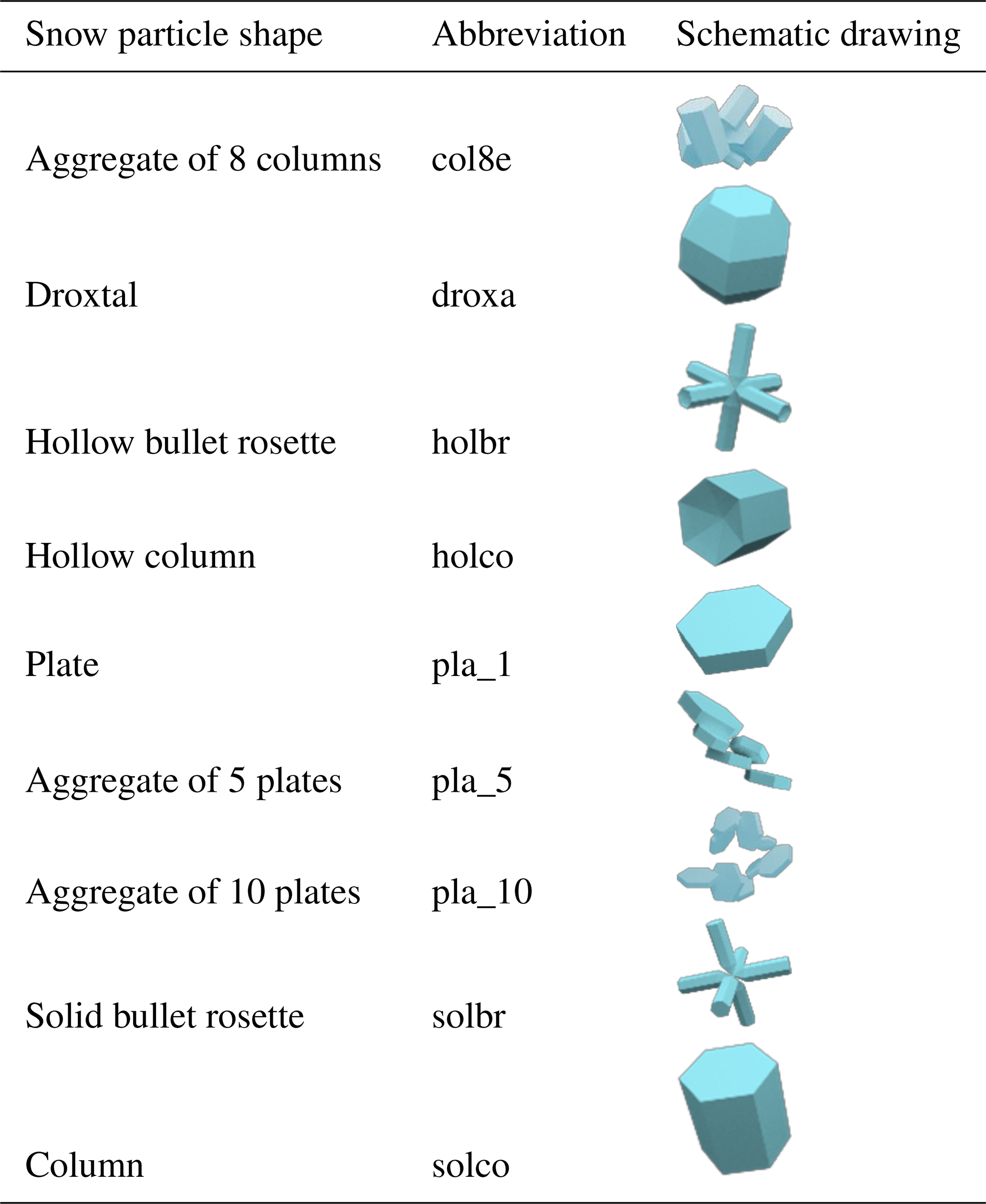
This paper presents a new retrieval algorithm to derive SGS, SPS and SSA from satellite observations. In a snow–atmosphere system, satellite-observed TOA reflectances are affected by numerous snow and atmospheric parameters. The parameters, which will be estimated in the framework of the eXtensible Bremen Aerosol/cloud and surfacE parameters Retrieval (XBAER) algorithm, will be called the target parameters. Other parameters, which the TOA reflectance also depends on, will be called the model parameters. In the case of the XBAER algorithm, the target parameters are SGS, SPS and SSA, whereas the model parameters are aerosol loading, cloud optical thickness and gaseous absorption. Throughout the paper, SGS will be characterized by an effective radius. Following Baum et al. (2011), the effective radius is defined as , where V and Ap are the volume and average projected area, respectively. As can be seen in the case of a spherical particle, the effective radius is equal to the radius of the sphere. The general concept of the retrieval algorithm is to use simultaneously spectral and angular reflectance measurements, which are sensitive to SGS and SPS. The spectral channels used in the XBAER algorithm are 0.55 and 1.6 µm. Both nadir and oblique observation directions from the Sea and Land Surface Temperature Radiometer (SLSTR) are used. An optimal SGS and SPS pair is achieved by minimizing the difference between measured and simulated atmosphere-corrected surface reflectances. SSA is then calculated based on the retrieved SGS and SPS. Nine predefined SPSs (aggregate of 8 columns, droxtal, hollow bullet rosette, hollow column, plate, aggregate of 5 plates, aggregate of 10 plates, solid bullet rosette, column) (Yang et al., 2013; see Table 1) are used to describe the snow optical properties and to simulate the snow surface reflectance at 0.55 and 1.6 µm at two observation angles.
Table 1Snow particle shape provided in Yang et al. (2013) database. The abbreviations introduced here will be used later.
There are three points we would like to emphasize to avoid misunderstandings between the snow science community and remote sensing community.
-
Usage of the Yang et al. (2013) database for ice crystals in the air (ice cloud) and on the ground (snow). The optical properties of ice crystals presented by Yang et al. (2013) have been widely used to study ice clouds. In recent publications, it has been demonstrated that they can also be used for snow studies (Räisänen et al., 2015; Pirazzini et al., 2015; Saito et al., 2019; Schneider et al., 2019; Pohl et al., 2020b). In fact, the single-scattering properties of ice crystals in the Yang et al. (2013) database are determined solely by the given particle size, shape and refractive index. They can be used to describe the optical properties of both snow particles and ice cloud particles when the particle models represent the aforementioned optical/physical properties (Saito et al., 2019; Masanori Saito, personal communication, 2021).
-
Snow particle shape observed from field measurements and derived from satellite observations. For scientists working in a laboratory or on campaign-based studies, the best way to obtain an image of snow is to use an X-ray microtomography or confocal scanning optical microscope/scanning electron microscope (Hagenmuller et al., 2016; Baker et al., 2019; Ian Baker, personal communication, 2021). In a field measurement and its related application areas (e.g., calculation of snow albedo), a spherical-shape assumption is widely used because it is easier to derive other snow properties such as SSAs and snow albedo based on this assumption, compared to using other more complicated shapes (see Appendix). The assumptions of a spherical and non-spherical shape have much less impact on the estimation of snow albedo compared to the bidirectional reflection features of snow (Grenfel and Warren, 1999; Dumont et al., 2010), because SPS has a significant impact on the ice crystal phase function while it has a relatively weak impact on the snow extinction/absorption coefficient (Jin et al., 2008). However, the spherical shape cannot be used to provide typical bidirectional reflection features of snow with the required accuracy (Jin et al., 2008; Dumon et al., 2010; Jiao et al., 2019), which is the fundamental basis for deriving snow properties from satellite remote sensing techniques. Thus, more complicated SPSs, such as those proposed by Yang et al. (2013), are recommended to use in the simulations of the angular distribution of snow reflectance. Besides, both snow albedo and directional reflectance are affected by other factors such as how single particles aggregate.
-
SGS and SSA. Although what the definition of a snow grain constitutes is an ongoing debate in different communities, SGS and SPS are two fundamental inputs for any radiative transfer model, which is the basis for the satellite retrievals (Langlois et al., 2020). Typically, the SSA is preferable within the snow science community because SSA is commonly used in further applications based on field measurements. We note, however, according to the definition of SSA, for a given SPS, a unique relationship between SGS and SSA can be derived. SPS is the intermediate but fundamental parameter needed to retrieve SSA in our XBAER algorithm.
This paper is structured as follows: observation characteristics of SLSTR and the laboratory measurements used for sensitivity studies are described in Sect. 2. The theoretical background and the ice crystal database (Yang et al., 2013) are presented in Sect. 3. Section 4 describes the eXtensible Bremen Aerosol/cloud and surfacE parameters Retrieval (XBAER) algorithm. The results of a comprehensive sensitivity study using SCIATRAN (Rozanov et al., 2014) simulations are presented in Sect. 5. The conclusions are given in Sect. 6.
2.1 SLSTR instrument
The satellite data will be used in two ways throughout the two companion papers (this paper and Mei et al., 2021). In the first part, we perform a statistical analysis of the SLSTR observation/illumination geometries to select realistic settings for the sensitivity study. In the companion paper, the satellite measurements will be used as the inputs of the XBAER algorithm to derive the research satellite products of SGS, SPS and SSA.
The SLSTR instrument on board the European Space Agency (ESA) satellite Sentinel-3 is the successor of the Advanced Along-Track Scanning Radiometer (AATSR) instrument and is used to maintain continuity with the (A)ATSR series of instruments. SLSTR has the heritage of AATSR instrument characteristics, especially the dual-viewing observation capabilities and wavelength settings. In order to have a reasonable setting for observation/illumination geometries in the sensitivity study, we perform a statistical analysis of the SLSTR observation geometries (solar zenith angle, SZA; viewing zenith angle, VZA; relative azimuth angle, RAA), similarly to Mei et al. (2020a). This analysis is essential because (1) it provides a realistic setting of observation/illumination geometries in our sensitivity studies and (2) it helps us to have a complete understanding of the observation-/illumination-related surface/atmospheric properties. Here the definition of RAA has been harmonized with SCIATRAN (Rozanov et al., 2014); namely, the RAA value is equal to 0∘ under a strict glint condition. The statistical analysis has been performed using observations made over Greenland during April and September 2017. April and September are reported to be representative months of the Arctic (Mei et al., 2020a). Please note that these two months are picked to represent the SLSTR observation characteristic with a typical solar illumination angle; the change in underlying surface properties plays no role in such a selection. Figure 1 shows the frequency of SLSTR observation geometries. The upper panels show the SZA with SLSTR nadir and oblique observations for April and September. We can see that the SZA occurs frequently with a value of 70∘ for selected months. The VZA and RAA for oblique observation mode are typically around 55∘ and in a range of [110∘, 170∘], respectively. The observation geometries for nadir observation show relatively large variabilities due to larger swath width compared to for oblique observations (1400 vs. 700 km). Larger SZAs can be found especially at the edge of the swath. The VZA and RAA for oblique observation mode are typically in ranges of [0∘, 55∘] and [70∘, 140∘], respectively. According to the statistical analysis, a combination of SZA, VZA and RAA of 70, 30 and 135∘ for nadir observation and 70, 55 and 135∘ for oblique observation can be a reasonable setting for the SLSTR observation geometries for the sensitivity study.
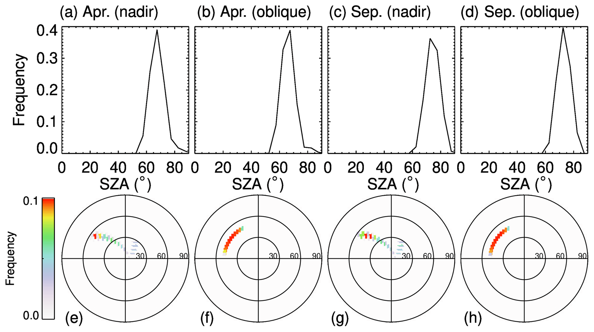
Figure 1Upper panels are the histograms of SZA for SLSTR observations: (a) nadir during April, (b) oblique during April, (c) nadir during September, and (d) oblique during September. Lower panels are the polar plots of (VZA, RAA) probability for AATSR observations: (e) nadir during April, (f) oblique during April, (g) nadir during September, and (h) oblique during September.
2.2 Laboratory measurements
Laboratory measurements of the bidirectional reflectance of snow samples contain important information about the dependence of the angular structure of snow reflection on the lighting geometry, wavelength and snow physical properties. The comparison of measured and modeled bidirectional reflectance helps to establish the conceptual ideas for the retrieval algorithm. For this comparison, we have selected measurements of fresh and aged snow samples presented by Dumont et al. (2010) and Peltoniemi et al. (2009), respectively.
The fresh snow sample, a cylinder of 30 cm diameter and 12 cm height, was taken from a new wet snow layer at Col de Porte (Chartreuse, France) at 1300 m above sea level during January 2008 (Dumont et al., 2010). The sample was stored in a cold room at −10 ∘C for 1 week to avoid metamorphic effects during the ensuing measurements. To obtain the bidirectional reflectance factor (BRF), the snow sample was illuminated by a monochromatic light source at an incidence zenith angle of 60∘. The spectral BRF between 500 and 2600 nm was measured at viewing zenith angles of 0, 30, 60, and 70∘ and relative azimuth angles 0, 45, 90, 135, and 180∘ by a spectrogonio radiometer developed at the Laboratoire de Planétologie de Grenoble, France, and using a Spectralon® and an Infragold® sample as a reference (see Dumont et al., 2010, for further details).
The aged snow sample, a cuboid of more than 10 cm height, was taken from an old dry snow layer at Masala, Finland, and brought into a warm laboratory. The spectral BRF between 350 and 2500 nm was measured during the aged process by the Finnish Geodetic Institute field goniospectropolariphotometer (FIGIFIGO) and using a Labsphere Spectralon® 99 % white reference plate. For illumination, a 1000 W Oriel Research quartz tungsten halogen lamp at a zenith angle of 60∘ was utilized (Peltoniemi et al., 2009). The spectral BRF was obtained at viewing zenith angles of up to 70∘ in 1∘ resolution and at relative azimuth angles of 0, 90, 130, 160, 180, 270, 310 and 340∘. The first and last measurements were made in the principal plane, indicating minor metamorphism in the snow layer during the measurement.
A comprehensive data library (Yang et al., 2013) containing the scattering, absorption and polarization properties of ice particles in the spectral range from 0.2 to 15 µm was used to calculate radiative transfer through a snow layer (Pohl et al., 2020b). A full set of single-scattering properties is available for nine ice crystal habits presented in Table 1. The maximum dimension of each habit ranges from 2 to 10 000 µm in 189 discrete sizes.
The optical properties of ice crystals depend on wavelength, ice crystal size and shape. Maximal dependence of the single-scattering albedo on the particle size is observed in the spectral ranges where ice absorption cannot be neglected. The asymmetry factor depends on the particle size for the whole spectral range. This dependence can be weaker or stronger at a selected wavelength depending on SPS (see Yang et al., 2013, for details).
To better illustrate the impact of SGS and SPS on the radiative transfer through a snow layer, we have calculated the reflectance of the snow layer consisting of droxtals, aggregates of 8 columns, hollow columns and plates with crystal surface roughness conditions as severely roughened. The simulations of snow reflectance were performed using the radiative transfer package SCIATRAN (Rozanov et al., 2014). The snow layer was defined as a layer directly over a black surface, with snow optical thickness of 500 and a snow geometrical thickness of 1 m. The snow layer is assumed to be vertically and horizontally homogeneous without any surface roughness and composed of monodisperse ice crystals. The impact of snow impurities and scattering/absorption processes in the atmosphere was neglected at this stage. The reflectance of the snow layer as a function of the effective radius of ice crystals at wavelengths of 0.55 and 1.6 µm is presented in Fig. 2. The calculations were performed for typical SLSTR instrument observation/illumination geometries (see Sect. 2.1), with SZA, VZA and RAA equal to 70, 30 and 135∘ (scattering angle 129∘).

Figure 2Reflectance of snow layer at 0.55 and 1.6 µm calculated assuming different SPSs. Observation/illumination geometry: SZA, VZA and RAA were set to 70, 30 and 135∘, respectively.
There are a couple of criteria we considered for the selection of the optimal wavelengths (0.55 and 1.6 µm) in the XBAER algorithm, for the purpose of creating a long-term satellite snow property dataset with good and stable accuracy.
-
We took the overlap channels between AATSR and SLSTR because a consistent long-term satellite snow dataset is possible only when the same algorithm can be applied to both AATSR and SLSTR instruments. In particular, the overlap channels between AATSR and SLSTR are 0.55, 0.66, 0.87, 1.6, 3.7, 10.85 and 12 µm.
-
Picking up wavelengths for which the contribution of thermal emission can be ignored, then 0.55, 0.66, 0.87 and 1.6 µm remain.
-
Deleting the channel 0.66 µm to avoid the potential impact of O3 absorption, after that, 0.55, 0.87 and 1.6 µm remain.
-
We take into account that the retrieval algorithm is a two-stage algorithm; namely, first it uses channels with minimum impact of the ice crystal shape to retrieve the grain size, and then it selects the shape using channels with minimum impact of grain size. Accounting for the fact that the 0.87 µm channel is impacted by both size and shape, 0.55 and 1.6 µm channels were picked up for the retrieval.
The right panel of Fig. 2 demonstrates the strong dependence of the snow layer reflectance at 1.6 µm on the SGS. One can also see that the dependence of snow reflectance on SPS cannot be neglected. In particular, the same reflectance can be obtained with a combination of different SGS and SPS. For instance, one can see from the right panel of Fig. 2 that the reflectance of the snow layer consisting of droxtals with SGS=200 µm or of plates with SGS=65 µm equals ∼0.035 in both cases. Thus, assuming different SPSs, the values of retrieved SGS can differ three times. The left panel of Fig. 2 demonstrates the dependence of the snow layer reflectance at 0.55 µm on SGS and SPS. It can be seen that the dependence of reflectance on SGS is very weak for droxtals and aggregates of 8 columns. However, reflectance at 0.55 µm decreases with an increase in SGS for hollow columns and plates. The weak oscillations for the reflectances at 0.55 µm can be explained by the joint impact of oscillations in the single-scattering albedo and elements of the scattering matrix presented in the original database. Although the reason for the oscillation in the database is unclear, it is unlikely due to physical phenomena (Masanori Saito, personal communication, 2021).
To illustrate this point, the dependence of the phase function at a 129∘ scattering angle on SGS is shown in the left panel of Fig. 3. The phase functions (F11 element of the scattering matrix) were extracted from the original database. According to the left panel of Fig. 3, the dependence of snow surface reflectance at 0.55 µm on SGS and SPS is caused mainly by the phase function of ice crystals. Weak oscillations can also be found.
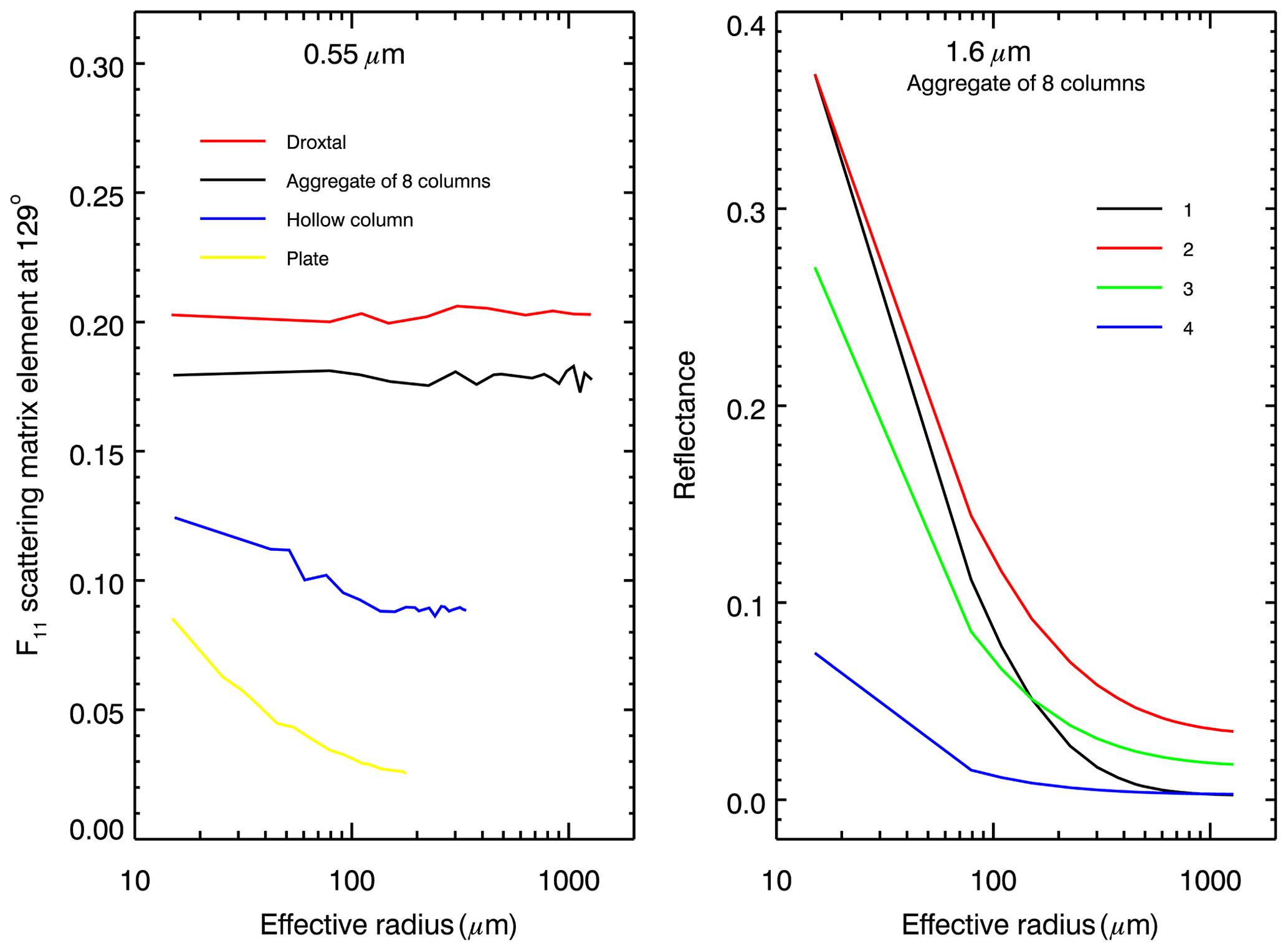
Figure 3Left panel: phase function at 0.55 µm for scattering angle of 129∘, extracted from the original database (Yang et al., 2013) as a function of effective radius. Right panel: reflectance of snow layer at 1.6 µm consisting of aggregates of 8 columns, calculated assuming that (1) phase function depends on the effective radius (black line), (2) phase function is constant corresponding to the effective radius of 15 µm (red line), (3) same as (2) but for effective radius of 150 µm (green line) and (4) same as (2) but for effective radius of 1150 µm (blue line).
The above analysis shows that accurate retrieval of SGS requires adequate information about SPS and accounting for the dependence of the phase function on SGS. To better illustrate the impacts of SGS on the ice crystal phase function, we calculated reflectance at 1.6 µm with different SGS values. The right panel of Fig. 3 represents the reflectance of the snow layer, consisting of aggregates of 8 columns, calculated accounting for the dependence of the phase function on the effective radius (black line) and assuming a constant phase function for three selected effective radii equal to 15, 150 and 1150 µm (red, green and blue lines, respectively). It can be seen that the accurate simulation of snow reflection requires accounting for the dependence of the phase function on SGS.
The main findings of the presented investigations can be formulated as follows:
-
Reflectance of a snow layer depends on both SGS and SPS.
-
Accurate simulation of snow surface reflectance requires accounting for the dependence of the phase function on SGS.
-
Spectral channels in the visible spectral range are more sensitive to SPS compared to SGS.
-
Spectral channels in the near-infrared spectral range are more sensitive to SGS compared to SPS.
Although the global classification of snow crystal, ice crystal, and solid-precipitation particles suggested in Kikuchi et al. (2013) consists of 121 particle types, we restrict ourselves, in the retrieval algorithm, to nine shapes of ice crystals, for which optical characteristics are represented in the database (Yang et al., 2013). And these nine shapes have been proven, especially from satellite observations, to be able to reproduce typical wavelength/angular features of snow reflectance in reality (Räisänen et al., 2015; Pirazzini et al., 2015; Saito et al., 2019; Schneider et al., 2019; Pohl et al., 2020b). To further illustrate that the selected dataset is able to reproduce the BRF of different snow types, we compared the simulated and measured BRF of fresh (Dumont et al., 2010) and aged (Peltoniemi et al., 2009) snow samples. To reproduce the spectral BRF by SCIATRAN, we use the setup described above in this section and adjust the SGS for each SPS by minimizing the deviation between simulated and measured reflectance at 1.6 µm. Figure 4 shows the simulated BRF in the principal plane at 0.55 µm of fresh and aged snow samples, as well as the respective measurements. The BRF is defined as , where I is the reflected radiance and F is the incident irradiance. According to Fig. 4a, for fresh snow, plates are the best shape to reproduce the measured BRF in the vicinity of the forward scattering peak but plates underestimate the BRF at higher viewing zenith angles in the backscattering region. Here, shapes of hollow bullet rosette, hollow column and aggregate of 10 plates exhibit better potential to simulate the fresh-snow-layer BRF. In the case of aged snow, shapes of solid and hollow column, hollow bullet rosette, and aggregate of 5 and 10 plates provide BRF values in conformity with respective measurements. However, they slightly underestimate the BRF at high zenith angles in the backscattering region where aggregates of 8 columns can simulate the aged-snow BRF better.
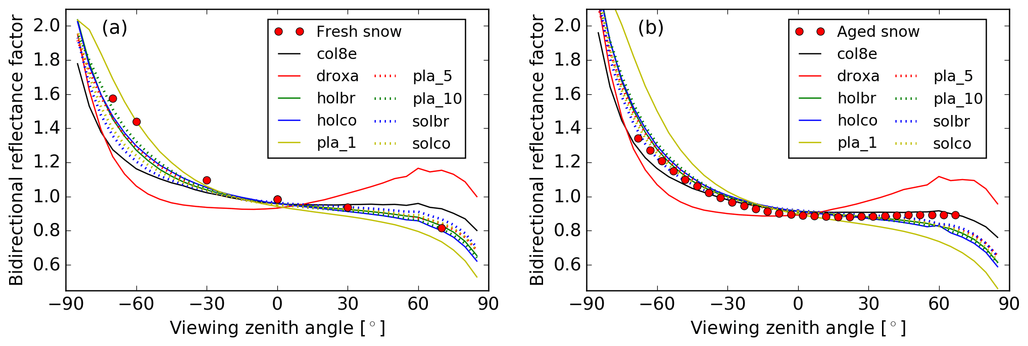
Figure 4The comparison of angle dependence of laboratory-measured and simulated snow reflectance: (a) fresh snow sample and (b) aged snow sample. Symbols are measurements and lines are simulations with SCIATRAN, assuming different SPSs (see legend).
The above analysis demonstrates that the selected database of SPS can be used successfully to reproduce measured BRF of both fresh and aged snow samples. Similar results were obtained by Pohl et al. (2020b). In this paper, the top-of-atmosphere BRF at 865 nm derived from POLarization and Directionality of the Earth's Reflectances 3 (POLDER-3) on Polarization & Anisotropy of Reflectances for Atmospheric Sciences coupled with Observations from a Lidar (PARASOL) measurements over a pure snow surface in Greenland (70.5∘ N, 47.3∘ W) on 6 July 2008 were compared with the SCIATRAN simulations, using droxtals, solid bullet rosettes and solid columns.
According to the above analysis, we can formulate the general algorithm to retrieve SGS and SPS from satellite observations. Satellite provides the wavelength-dependent TOA reflectance. For a given SGS and SPS pair, the minimization between satellite-observed TOA reflectance and theoretical simulation is performed. The optimal SGS and SPS are obtained when the difference between observations and simulations reaches the predefined criteria. The SSA is then calculated by the retrieved SGS and SPS.
The retrieval algorithm consists of three stages. The first stage includes the estimation of SGS using the effective Lambertian surface albedo after atmospheric correction for selected observation geometries and wavelengths. This step is performed based on the path radiance representation (Mei et al., 2017), in which the TOA reflectance can be described by the contribution from the atmosphere and the interaction between atmosphere and surface. The inverse to derive the surface reflectance from the satellite-observed TOA reflectance is called the atmospheric correction. And due to certain assumptions in the path radiance representation, the derived surface reflectance is equivalent to the effective Lambertian surface albedo. The estimation of SGS is obtained solving the following minimization problem with respect to the effective radius, r, of snow crystals:
Here, Ae and Rs(r) are two vectors whose components are the effective Lambertian surface albedo and the simulated snow reflectance, respectively. The dimension of these vectors is the number of wavelengths times the number of viewing directions.
The simulation of snow reflectance (components of vectors Rs(r)) was performed using the radiative transfer package SCIATRAN (Rozanov et al., 2014) as described in Sect. 3. The optical properties of nine SPSs, listed in Table 1, were used for radiative transfer calculations.
The minimization problem formulated by Eq. (1) was solved separately for each SPS using Brent's method (Brent, 1973). The solution of the minimization problem for each crystal habit is characterized by the following residual:
where is the solution of minimization problem given by Eq. (1) for the ith shape of the ice crystal particle.
The second stage is the selection of such i values (SPS) for which Δi is minimal. This completes the retrieval process and enables the optimal SGS and SPS to be obtained.
The third stage is to calculate SSA for the retrieved SGS and SPS. To this end, let us rewrite the SSA introduced above in the following equivalent form:
where r is the effective radius. According to Cauchy's surface area formula (Cauchy, 1841; Tsukerman and Veomett, 2016), the average area of the projections of a convex body is equal to the surface area of the body, up to a multiplicative constant. In our case, this results in At=4Ap and SSA for convex particles such as droxtals, solid columns and plates is equal to . In the case of non-convex particles, the calculation of SSA requires information about total area At. Although the database given by Yang et al. (2013) does not contain information about At, the total area of non-convex particles can be calculated employing the geometric parameters of ice crystal habits presented in Table 1 of Yang et al. (2013). Here we take a typical SPS, aggregate of 8 columns, as an example, to show the difference between SSA calculated assuming convex and non-convex particles.
According to Masanori Saito (personal communication, 2021), the parameters L and a of the aggregate of 8 columns (see Fig. 3 in Yang et al., 2013, for details) can be obtained by scaling with respect to the maximum dimension, D. To find these values for different maximal dimensions, we calculate at first the volume of the aggregate of 8 columns corresponding to parameters a and L on a relative scale as given in Table 1 of Yang et al. (2013).
Using the database of Yang et al. (2013), one can obtain the maximal dimension, Dr, corresponding to the volume, Vr. Introducing the scaling factor, , we have the semi-width and length for the aggregate with the maximal dimension Dk:
The total surface of the aggregate on a relative scale is given by
Accounting for Eq. (5), we have
Having obtained the total area, one can calculate SSA as the total surface area of a material per unit of mass:
Comparing SSA of a convex particle equal to with the result given by Eq. (8), one can easily notice the difference in SSA calculated from different SPSs using the same SGS. The details of such calculations for other non-convex ice crystal habits are given in the Appendix.
The relationship between SSA and SGS for different SPSs is presented in Fig. 5. According to Fig. 5, an almost inverse linear relationship between SSA and SGS can be found. The lines, representing droxtal, plate and column, overlap, indicating the same SSA for convex particles. For other SPSs with the same SGS, SSA is larger compared to convex faceted particles. SSA is restricted to the range of 0–100 m2 kg−1 in this investigation (Picard et al., 2009). For example, for SGS=100 µm, the SSA is 32.7 m2 kg−1 for convex faceted particles, whereas SSAs for aggregate of 8 columns, hollow bullet rosette, hollow column, aggregate of 5 plates, aggregate of 10 plates and solid bullet rosette are 44.2, 43.4, 37.7, 74.4, 66.8 and 35.6 m2 kg−1, respectively. The relative differences range from 9 %–128 %, depending on the SPS. Taking into account the definition of SSA, one can derive the following relationship between SSA convex and non-convex particles: , where subscript c and nc denote convex and non-convex particles, respectively. The obtained results reveal that for all non-convex ice crystals under consideration, and the ratio weakly depends on the SGS.
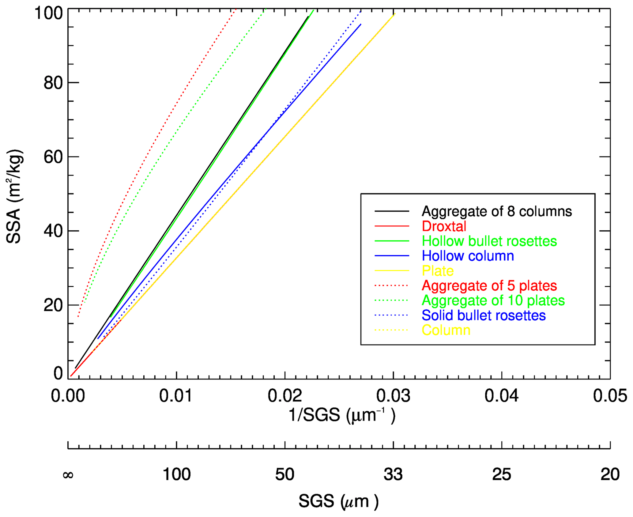
Figure 5Relationship between SGS and SSA for different SPSs. For a better illustration, the realistic range of specific surface area is limited to 100 m2 kg−1.
The accuracy of any retrieval algorithm depends not only on measurement errors but also on the uncertainty in parameters which cannot be retrieved. In our case, such parameters are ice crystal roughness, aerosol contamination and cloud contamination. The impacts of these factors on XBAER-derived SGS and SPS have been investigated and will be discussed in this section. The TOA reflectances at selected channels (0.55 and 1.6 µm) and observation directions for SZA, VZA and RAA of 70, 30 and 135∘ for nadir and 70, 55 and 135∘ for oblique, respectively, were calculated using the radiative transfer model SCIATRAN. The details of each scenario will be presented in the corresponding sub-section below.
5.1 Impact of snow particle shape
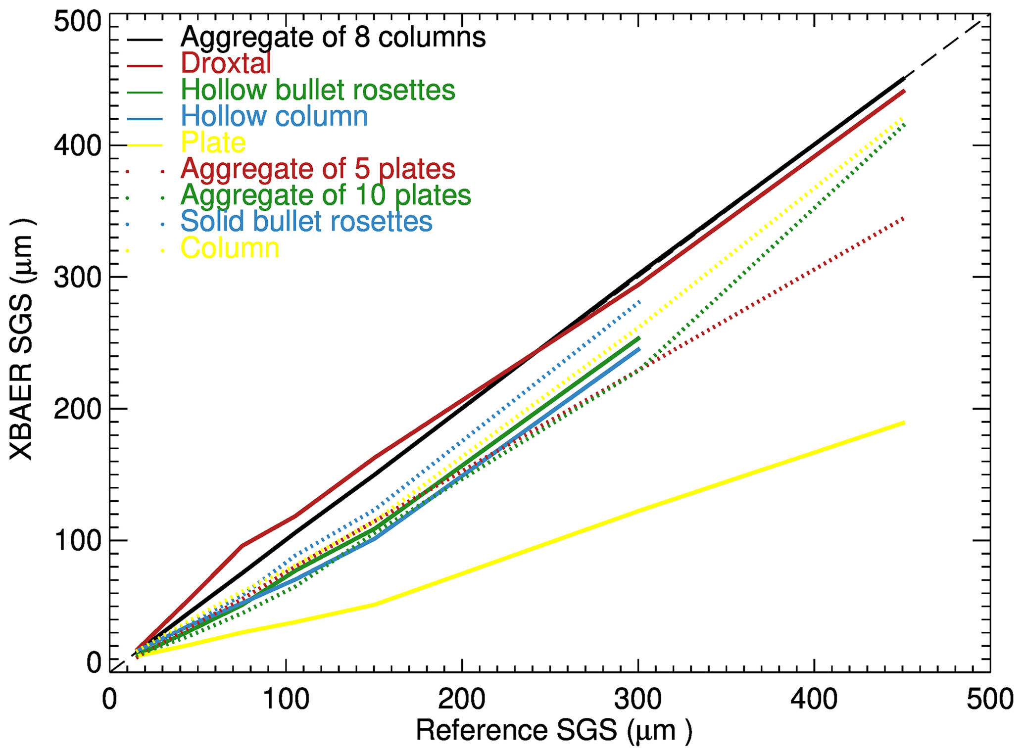
Since the first stage of the XBAER algorithm is to estimate the SGS assuming a given SPS, it is reasonable to investigate the impact of SPS on the retrieval of SGS. The TOA reflectances of a snow layer at 0.55 and 1.6 µm with the above-given observation geometries were calculated using the following settings for snow layer and atmospheric parameters:
-
Snow layer. This consists of ice crystals with SPS set to be severely roughened aggregates of 8 columns and maximal dimensions [100, 300, 500, 700, 1000, 2000, 3000, 5000] µm, which corresponds to SGS [15, 45.1, 75.2, 105.3, 150.4, 300.8, 451.3, 752.1] µm.
-
Atmosphere. This is excluded.
The simulated snow reflectances were used as components of vector Ae in Eq. (1). Nine SPSs from the database presented in Yang et al. (2013) are used sequentially in the retrieval process. The atmospheric correction is not performed because the atmosphere is excluded in the forward simulations. This enables avoiding additional errors caused by the atmospheric correction and estimates the pure effect of SPS on the retrieval results. Figure 6 shows the impact of the SPS on SGS retrieval. Different colors and line styles indicate different ice crystals used in the retrieval process. The solid black line represents the retrieved SGS assuming the SPS in the retrieval process is the same as in forward simulations. This line agrees well with the 1:1 line, indicating that the retrieval algorithm has been implemented technically correctly. According to Fig. 6, one can see both underestimation and overestimation of SGS depending on the SPS used in retrieval. However, in most cases, an incorrect SPS leads to an underestimation of SGS. In particular, the maximal effect can be seen when ice crystals of plate shape, rather than of the correct aggregate of 8 columns, is used (solid yellow line). This result can be easily explained coming back to the right panel of Fig. 2. Indeed, one can see that the same reflectance of the snow layer can be obtained using the plate shape, instead an aggregate-of-8-columns shape, with a significantly smaller SGS. These results reveal that the SPS is an important parameter affecting the accuracy of retrieved SGS.
5.2 Impact of SGS and SPS on SSA
Since the SSA is obtained from the retrieved SGS and SPS, an understanding of how the error in SGS and/or SPS propagates to the SSA will provide helpful information to understand the retrieved SSA. Figure 7 shows the impact of SGS (left) and SPS (right) on XBAER-retrieved SSA. The relative error in SGS, , is propagated to the relative error in SSA as , and it is independent of the reference SSA. The left panel of Fig. 7 depicts εSSA corresponding to ±0.16 of εr. One can see that this results in 19 % and −13.8 % of SSA relative errors, which are presented as the upper and lower error boundaries in the left panel of Fig. 7. The systematical error of ±16 % for SGS was obtained as the maximal relative difference between XBAER-retrieved SGS and both in situ and aircraft-measured SGS (as presented in the companion paper – Mei et al., 2021). This represents the worst case of SGS error propagation into SSA.
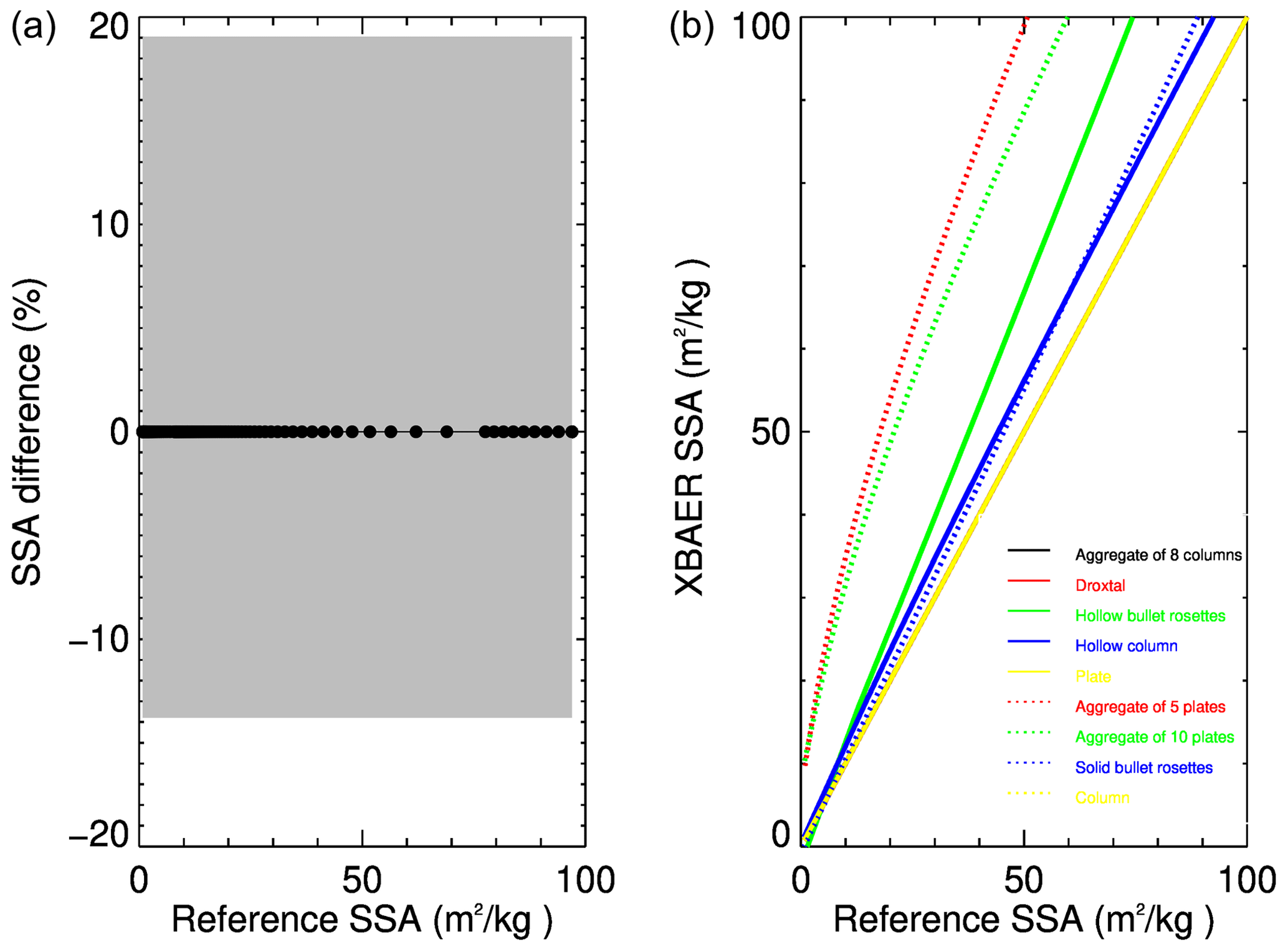
Figure 7Impact of SGS and SPS on the retrieval of SSA. (a) SGS errors – the black line with dots indicates the 0 difference for accurate SGS for aggregate of 8 columns, and the grey area indicates the relative error in SSA introduced by a 16 % error in SGS; (b) SPS selection – different color and line styles indicate different SPSs used in the calculation of SSA while the true SPS is set to be “plate” or other convex particles.
The impact of SPS on SSA is demonstrated in the right panel of Fig. 7. As a reference shape, we have selected in this case the plate, which provides the same SSA as other convex particles. One can see that the SSA of non-convex particles overestimates the SSA of convex particles, which is in line with the results presented in Sect. 4. For instance, for the same SGS, the SSA for aggregate of 8 columns (non-convex particle) is about 3 times larger than that for doxtal (convex particle). Since the assumption of the sphere (convex particle) is used to measure SSA in-field measures (Gallet et al., 2009; Nick Rutter, personal communication. 2021), such as observations from SnowEx, the retrieval results of SSA from XBAER will be systematically larger than field measurements in the case of non-convex particles even if the retrieved and measured SGSs are similar. However, a detailed discussion with respect to uncertainty in the campaign-based measurement is out of the scope of this paper.
5.3 Impact of ice crystal surface roughness
Although the surface roughness of ice crystals is not too severe for snow compared to ice cloud due to basic thermodynamics (Colbeck, 1980, 1983), the ice crystal surface roughness (ICSR), indicating ice crystal surface texture, may still be important for the retrieval of snow properties from optical sensors such as SLSTR. The ICSR has been used as a new variable in model simulation (Järvinen et al., 2018). Retrieval algorithms of ice cloud parameters are frequently based on the assumption that the ice crystal surface is smooth (Kokhanovsky et al., 2019). This assumption can however introduce large uncertainty in the ice cloud retrieval parameters and, as a consequence, lead to misunderstanding the impacts of ice clouds on global climate change (Järvinen et al., 2018). However, this issue has not yet been discussed for snow. In general, ice crystal surfaces are rougher in clouds than in snow layers due to metamorphism processes (Colbeck, 1980, 1983; Ulanowski et al., 2014). The investigation of the impact of ICSR on retrieval of snow properties provides valuable information to understand the XBAER algorithm. The ICSR according to Yang et al. (2013) is defined similarly to the definition suggested by Cox and Munk (1954) for the roughness of the sea surface. A parameter σ describes the degree of ICSR. The σ values 0, 0.03 and 0.5 are for three surface roughness conditions: smooth, moderate roughness and severe roughness. And only the above three values are available in the Yang et al. (2013) database. The snow layer reflectances were used as components of the vector Ae in Eq. (1) in the same way as in Sect. 5.1.
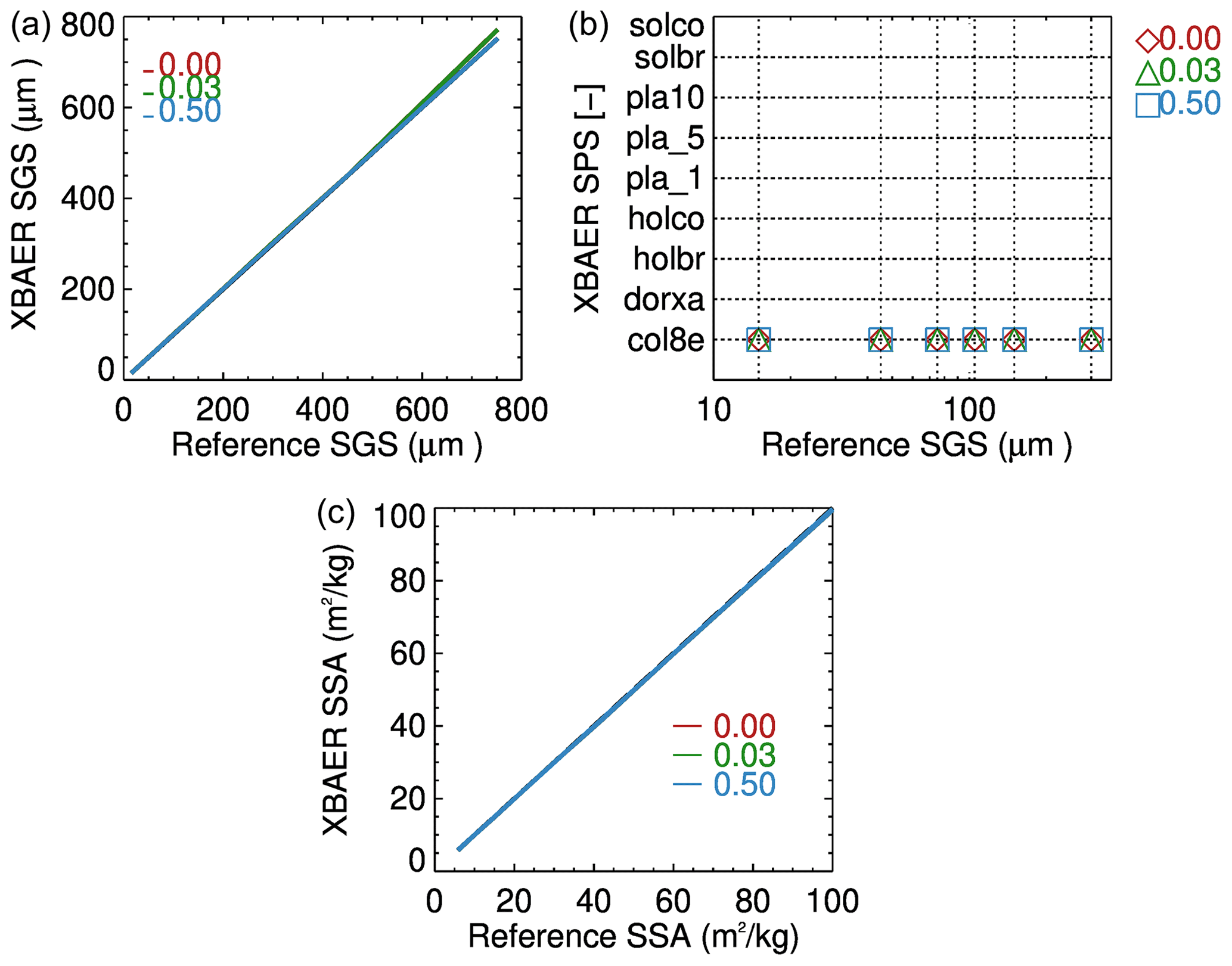
Figure 8Impact of ice crystal surface roughness (ICSR) on the retrieval of SGS (a), SPS (b) and SSA (c). Different colors indicate different ICSRs used in the retrieval.
Figure 8 shows the impact of ICSR on the retrieved SGS, SPS and SSA. The impact of ICSR on SGS and SSA are relatively small for SGSs smaller than ∼300 µm. Ignoring the impact of roughness leads, in general, to a slight overestimation of SGS and an underestimation of SSA. The absolute errors in SGS and SSA introduced by ICSR range from 0.3 %–3 %, depending on SGS. Due to the inverse almost linear relationship between SSA and SGS, as presented in Fig. 5, for the same SPS, an overestimation of SGS leads to an underestimation of SSA. The slight overestimation can be found if less ICSR is taken into account in retrieval because the snow reflectance with the same SGS and SPS for ICSR=0.5 is larger than for ICSR=0.03 due to the lower asymmetry factor of ice crystals with more roughened surface roughness; thus the same surface reflectance observed by satellite requires a larger SGS for the case with ICSR=0.03 used in retrieval in contrast to ICSR=0.5 used in the forward simulation. However, as can be seen from the right panel of Fig. 8, the XBAER algorithm still retrieves the correct SPS ignoring the impact of roughness.
5.4 Impact of aerosol contamination
The impact of aerosols on the retrieval of snow properties using passive remote sensing can be important because there is limited aerosol information over the cryosphere (Mei et al., 2013a, b, 2020a; Tomis et al., 2015) to perform an accurate atmospheric correction. The use of MERRA-simulated AOT, although of good data quality, will still introduce potential aerosol contamination into the XBAER-derived snow properties. The impact of aerosols on snow property retrieval is much smaller over Arctic regions compared to middle–low latitudes (e.g., Canadian Arctic, Tibetan Plateau) due to large absolute uncertainty in the MERRA-simulated aerosols over middle–low latitudes in wintertime. A detailed comparison of how possible aerosol contamination may affect the retrieved snow properties will be included in the companion paper (Mei et al., 2021). In the companion paper, the comparison between satellite-derived and campaign-measured snow properties all over the world will be included. In order to have a better understanding of aerosol contamination on snow property retrieval, the TOA reflectances were calculated at 0.55 and 1.6 µm with the above-given observation geometries using the following settings:
-
Snow layer. This is the same as in Sect. 5.1.
-
Atmosphere. Aerosol type is set to be weakly absorbing (Mei et al., 2020b) with AOTs of [0.05, 0.08, 0.11]. Other atmospheric parameters are set according to the Bremen 2D chemical transport model (B2D CTM) for April at 75∘ N (Sinnhuber et al., 2009). It is worth noticing these three AOT values represent background, average and pollution conditions in the Arctic as suggested by Mei et al. (2020a, b).
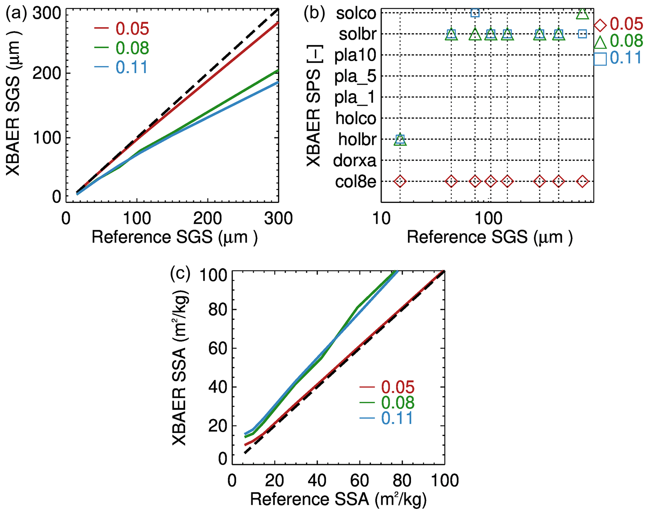
Figure 9Impact of aerosol contamination on the retrieval of SGS (a) SPS (b) and SSA (c). Different colors indicate different AOT used in forward simulations. No atmospheric correction is performed in the retrieval, black dash line is the 1:1 line.
Figure 9 shows the impact of aerosol contamination on the SGS (a), SPS (b) and SSA (c) retrieval. These results are obtained by introducing a 50 % error into AOT at the step of atmospheric correction and can be considered the worst case for impact of aerosol contamination on retrieved SGS, SPS and SSA. The surface reflectances estimated after employing the atmospheric correction were used as components of the vector Ae in Eq. (1). One can see that aerosol introduces systematic underestimation of retrieved SGS for the given scenarios and the magnitude of underestimation increases with the increase in AOT. For a typical background Arctic aerosol condition, with AOT=0.05, aerosol contamination introduces errors in SGS of less than 3 % for SGS≤150 µm and less than 7 % for µm. The maximal errors introduced by the aerosol contamination increase to 30 % and 37 % in the case of average and pollution conditions for AOT=0.08 and AOT=0.11, respectively. Please note that the AOT values in the Arctic can be even smaller than 0.05, for instance, AOT over Greenland. Thus, the analysis with respect to aerosol contamination is the worst case for a typical Arctic condition.
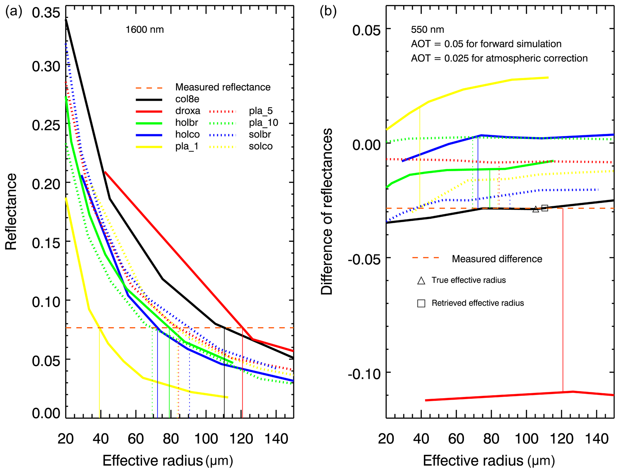
Figure 10Schematic representation of two stages of the retrieval process. (a) Determination of effective radius for each ice crystal form. (b) Selection of optimal SGS–SPS pair.
For the case of AOT=0.05, SPSs have been correctly retrieved for all SGS values, indicating that under a typical Arctic clean condition, the impact of aerosols is not so large as to disturb SPS retrieval. In order to demonstrate the two-stage retrieval process and illustrate the impact of aerosols, let us focus on Fig. 10. To facilitate the presentation, we consider the measurement of reflectance at 1.6 µm for a single observation direction (30∘) and at 0.55 µm for the difference in reflectance at two observation angles (30 and 55∘). This enables the avoiding of the minimization process given by Eq. (1) and represents the retrieval process in a simple graphic form. The left panel of Fig. 10 depicts the determination of an effective radius for each ice crystal form, assuming the correct shape is aggregate of 8 columns with an effective radius of 105.4 µm. Solid and dotted lines are the surface reflectance of the snow layer consisting of ice crystals with different forms, and the dashed line is the measured reflectance after the atmospheric correction. The obtained SGSs are in the range 40–120 µm, depending on the selected SPS, and presented in Fig. 10 by solid and dotted vertical lines. In the case of correct SPS selection (aggregate of 8 columns) the retrieved SGS is ∼110 µm. The right panel of Fig. 10 shows the second stage of the retrieval process, namely, the selection of an SPS for which the difference between the measured (dashed line) and simulated (solid black line) value is minimal. In the case under consideration the correct shape is selected with an effective radius of ∼110 µm.
For larger-AOT conditions, an inaccurate selection of SPS occurs for all SGS cases, indicating the remaining aerosol information is strong enough to decouple the aerosol contribution from the snow surface characteristic. Thus, a quality flag of SPS, associated with AOT, should be introduced into the retrieval of real satellite data. It is interesting to see that “solid bullet rosette” is the preferable SPS for very strong aerosol contamination cases. This is due to the similar scattering properties (shape) of ice crystals and weakly absorbing aerosols, defined in forward simulation. The impact of aerosol contamination, for typical Arctic conditions, introduces a less-than-5 % error into SSA. However, for large aerosol contamination, the around 30 % underestimation in SGS linearly introduced about 25 % overestimation in SSA, which agrees with the analysis as presented in Fig. 7.
Any cloud-screening method, especially over the cryosphere, may introduce cloud contamination for the retrieval of atmospheric and surface properties (Chen et al., 2014; Mei et al., 2017; Jafariserajehlou et al., 2019). Understanding of the cloud contamination will provide valuable information to interpret the retrieval results using the SLSTR instrument. To investigate the impact of cloud contamination, the following settings were used to perform the simulations of TOA reflectance:
-
Snow layer. This is the same as in Sect. 5.1.
-
Atmosphere. An aerosol-free atmosphere is used with other parameters as in Sect. 5.4. Additionally, vertically homogeneous ice cloud consisting of aggregates of 8 columns with an effective radius of 45 µm and optical thickness [0.1, 0.5, 1.0, 5] is set to be at the position of [5, 6] km.
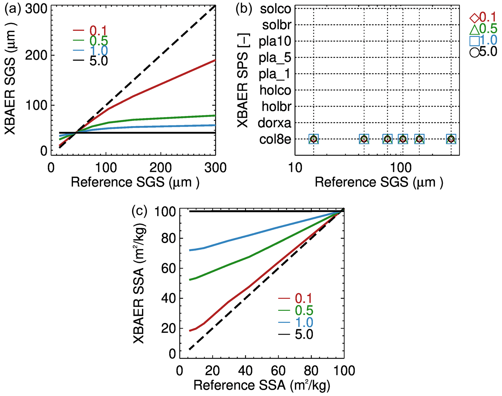
Figure 11Impact of cloud contamination on the retrieval of SGS (a), SPS (b) and SSA (c). Different colors indicate different COTs in forward simulations; dashed black line is the 1:1 line.
Figure 11 shows the impact of cloud contamination on XBAER-retrieved SGS (a), SPS (b) and SSA (c). The size of ice crystals in ice clouds is typically smaller than snow grain size (Kikuchi et al., 2013). Our statistical analysis of the ice crystal effective radius over Greenland shows an average value in the range of 30–50 µm, which is consistent with previous publications (King et al., 2013; Platnick et al., 2017). According to Fig. 11, an overestimation of SGS can be found for SGSs of less than 45 µm (cloud effective radius) and an underestimation of SGS can be found for SGSs larger than 45 µm. The magnitude of overestimation/underestimation increases with the increase in cloud optical thickness (COT). XBAER-derived SGS becomes saturated for COT larger than 0.5. Due to a limited photon penetration depth for optically thicker clouds (e.g., COT=5), the XBAER algorithm retrieves the effective radius of ice crystals in the cloud. This demonstrates that theoretically, the XBAER algorithm can retrieve an ice cloud effective radius without pre-processing of cloud screening. And this can be further used as post-processing to avoid cloud contamination.
The impact of the cloud on the retrieval of SPS is similar to the impact of aerosols considered above. In short, the cloud plays a larger role for larger SPSs (darker TOA) and this impact increases with the increase in COT. However, cloud with large COT can be much more easily detected and excluded by the cloud-screening algorithm (e.g., for the cases with COT>0.5). SPSs are correctly picked up due to the same SPS used for both the snow layer and the cloud layer. Similarly to the impact of aerosol, the underestimation of SGS introduced by the cloud leads to an overestimation of SSA (Fig. 11c). The increase in COT results in saturation of the ice cloud SSA, with a value of 100 m2 kg−1 in the case of aggregates of 8 columns.
The above theoretical investigations include all possible important factors affecting the accuracy of the XBAER algorithm. However, when applying the XBAER algorithm to the SLSTR instrument for real scenarios, two additional factors need to be considered as well: one is the impact of the instrument spectral response function (SRF), and the other one is the representativeness of the snow scenario for reality.
7.1 Impact of instrument spectral response function
-
Snow layer. This is the same as in Sect. 5.1.
-
Atmosphere. An aerosol-free atmosphere is used with other parameters as in Sect. 5.4.
The forward simulations are performed with and without the impact of the spectral response function (SRF). The SRFs for SLSTR at 0.55 and 1.6 µm are shown in Fig. 12. The retrieval is then performed ignoring the SRF. Figure 13 shows the impact of SRF on the retrieval of SGS, SPS, and SSA. For forward simulations without taking the SRF into account (labeled as No in Fig. 13), SGS, SPS and SSA are well received as expected. And this agrees with Fig. 6. However, ignoring the impact of the SRF introduces about 7 % uncertainties into the simulated surface reflectance, and this causes about a 5 %–7 % error in both SGS (overestimation) and SSA (underestimation). Taking the SRF into account leads to a smaller surface reflectance at 1.6 µm due to potential gas absorption at this wavelength and thus introduces an overestimation for SGS. However, due to a significantly smaller impact at 0.55 µm, the SRF does not play a significant role in the retrieval of SPS.
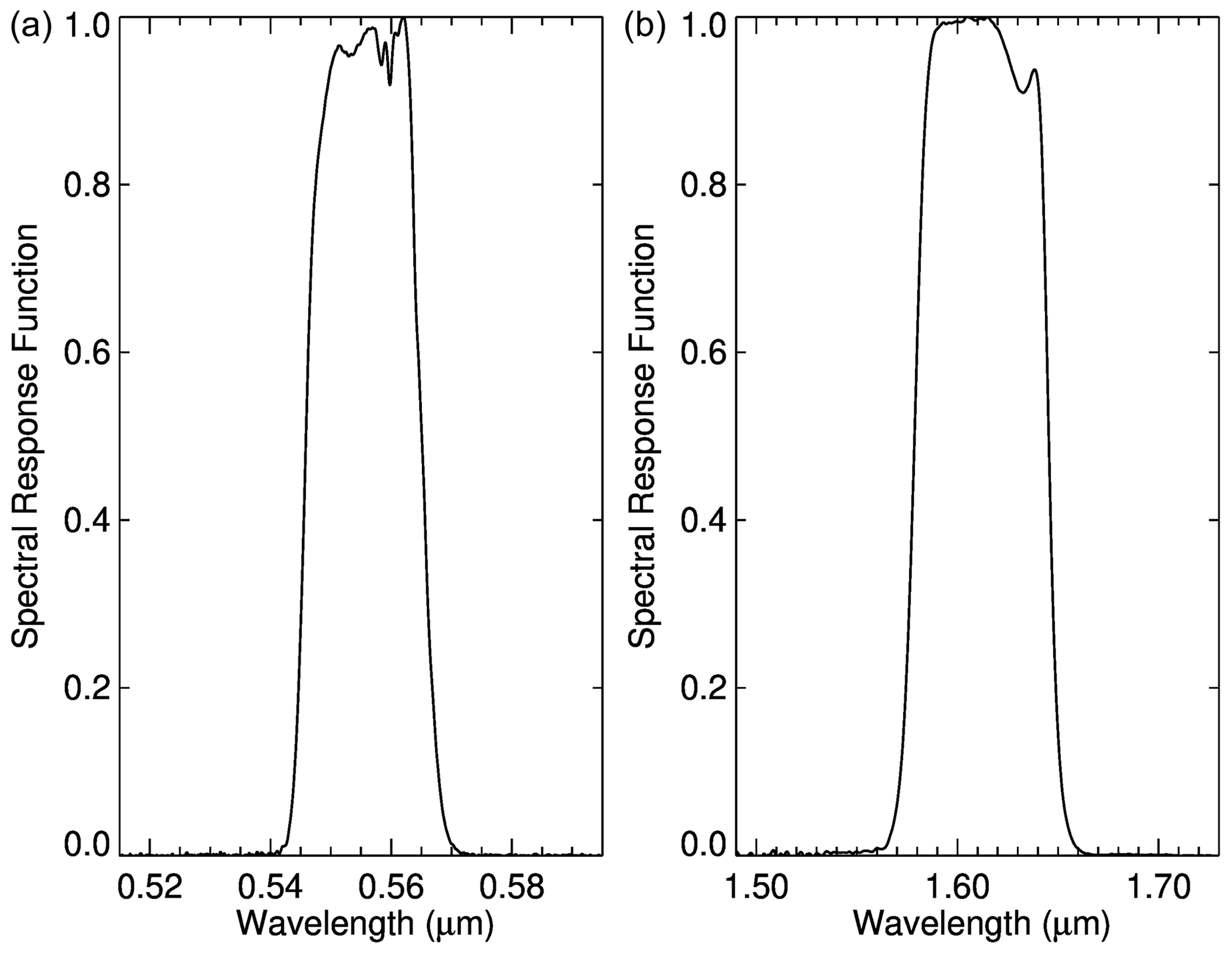
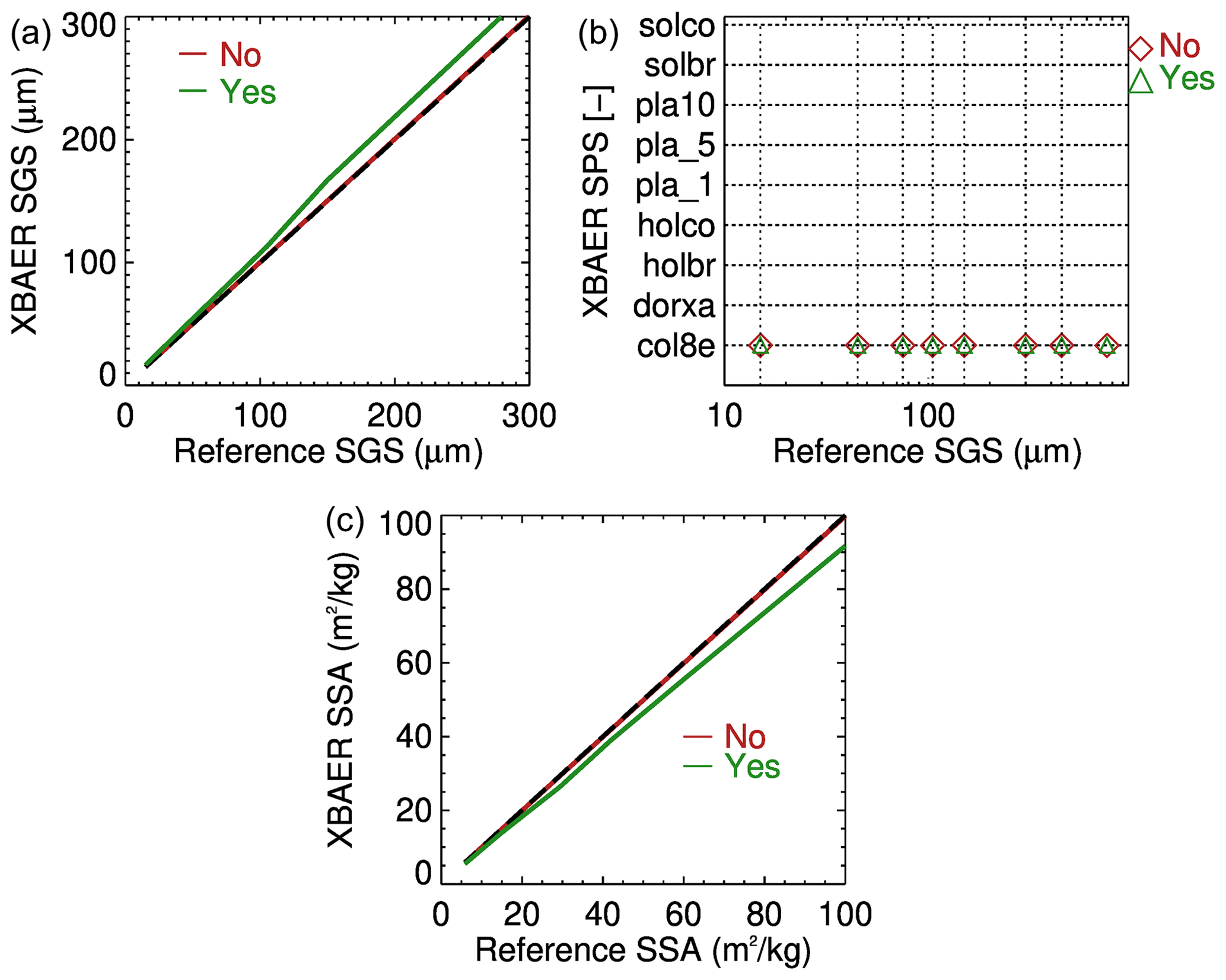
Figure 13Impact of SRF on the retrieval of SGS (a), SPS (b) and SSA (c). Different colors indicate retrieval results without (No) and with (Yes) the SRF in forward simulations; dashed black line is the 1:1 line.
7.2 Impact of snow inhomogeneities
In this section, a realistic model of the snow layer is represented by a vertically inhomogeneous, polydisperse ice crystal habit mixture. Following Saito et al. (2019), the gamma distribution with respect to the maximal dimension will be used to describe polydisperse properties:
Here, N is the number of ice particles per unit volume and G(D) is the gamma distribution function; i.e.,
where k and v are the shape and scale parameters, the normalization factor C is defined as
and Dmin and Dmax describe the minimal and maximum particle sizes in the distribution.
In order to introduce the vertical inhomogeneity, we use the measurement of snow density and equivalent optical diameter vertical profiles conducted during the SnowEx17 campaign. Accounting for the fact that the equivalent optical diameter cannot be directly used to define parameters of the gamma distribution, we use the vertical profile as a shape of the mode (most frequent value in a dataset); i.e.,
where De(z) is the measured vertical profile of equivalent optical diameter and D0(z) is the vertical profile of the mode. The mode near the top of the snow layer, D0(ztop), is assumed to be equal to 400 µm according to the measurement data reproduced by Saito et al. (2019) in their Fig. A1.
Taking into account the analytical expression of the mode via shape and scale parameters,
and the relationship between shape and scale parameters derived by Saito et al. (2019),
we can estimate parameters k and v of the gamma distribution corresponding to D0(z) given by Eq. (12).
The snow grain habit mixture (SGHM) model is used according to Saito et al. (2019). In particular, the particle habits include droxtal, solid hexagonal column and solid bullet rosette. The habit fraction, fh(D), as a function of the maximal dimension of the SGHM model is presented in Fig. 15b. The habit fraction is defined so that, for each D,
The selected SGHM model enables us to derive the total volume of ice per unit volume of air as
and ice water content (IWC)
where Vh(D) is the volume of each habit as given in the database of Yang et al. (2013) and ρice is the density of ice.
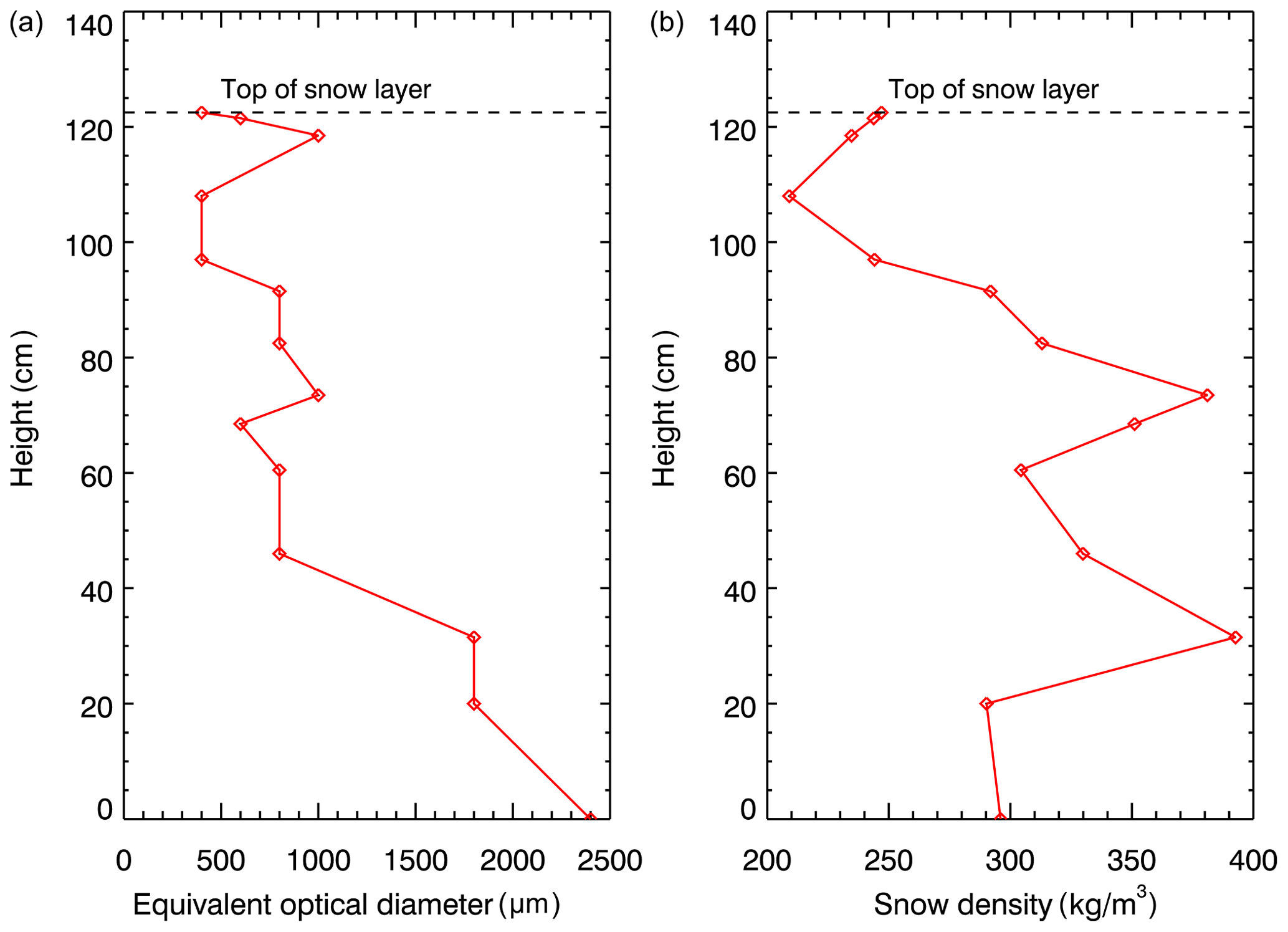
Figure 14Snow properties used for simulations to investigate the impacts of snow layer model on the XBAER retrieval (a) snow grain size profile and (b) snow density observed during the SnowEx17 campaign.
Taking into account the vertical profile if IWC is measured (see right panel of Fig. 14), we can obtain the vertical profile of the particle number density. Using Eqs. (16) and (17), we have
Summing up, we define the microphysical properties of the snow layer using the following model of particle size distribution:
where D0(z) and N(z) are given by Eqs. (12) and (18), respectively, and the shape parameter, k, is assumed to be altitude independent and set to 2.3.
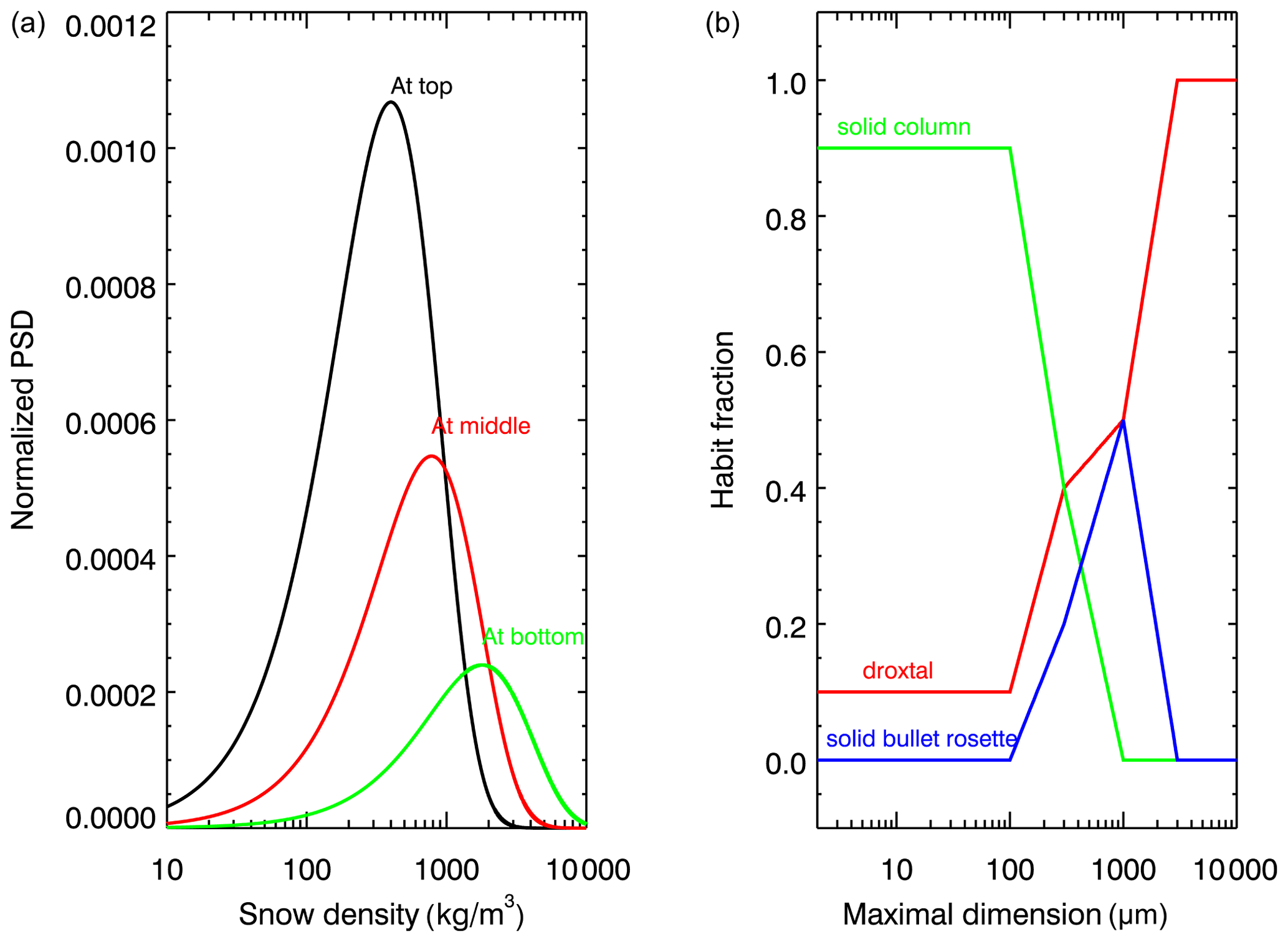
Figure 15Snow properties used for simulations to investigate the impacts of the habit mixture model on XBAER retrieval: (a) particle size distribution of snow grain size in snow layer and (b) habit fraction suggested by Saito et al. (2019).
The bulk single-scattering properties of the snow layer such as the extinction coefficient, scattering coefficient and scattering function are defined in the same way as proposed by Baum et al. (2011). For instance, the bulk extinction coefficient is calculated as
where σext,h(D) is the extinction cross section as given for each habit in the database of Yang et al. (2013).
The following settings are used to simulate the reference snow reflectance at wavelengths 0.55 and 1.6 µm:
-
Snow layer. This is a vertically inhomogeneous, polydisperse habit mixture and model as described above.
-
Atmosphere. This is excluded.
Using the simulated reflectances in the XBAER algorithm, we have retrieved SPS as droxtal with the maximal dimension equal to 740 µm. Taking into account that the model of particle size distribution (PSD) near the top of the snow layer is 400 µm and the mean value calculated as is equal to 708 µm, one can see that the retrieved maximal dimension is an estimation of the mean value of PSD near the top of the snow layer.
Since there is no single reference SGS value when a PSD is used, it is important to check the representativeness of XBAER-derived SGS. Accounting for the fact that the mode and mean values for a given PSD are two typical “effective” ways to describe a polydisperse medium, we compared reflectances of the snow layer calculated assuming PSD in the form of a gamma distribution and assuming a monodisperse medium with SGS equal to the mode or to the mean of the selected PSD. In order to simplify analysis, we consider vertically homogeneous snow layer consisting of only single-particle habit. The calculations of reflectance were performed for severely roughened aggregate-of-8-column and droxtal particles setting the shape parameter, k, equal to 2.3 and the model equal to [100, 300, 500, 700, 1000, 2000, 3000, 5000] µm.
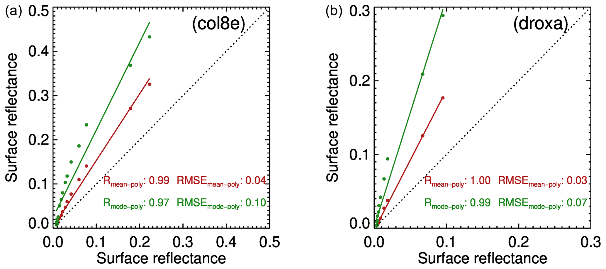
Figure 16The comparison between simulated snow reflectance using a mono- and polydisperse snow model consisting of aggregate of columns (a) and droxtal (b). In the case of the monodisperse model, the SGS is assumed to be the mean and mode value of PSD at the top of the snow layer (see Fig. 14a). The reference value is shown on the x axis.
Figure 16 shows the comparison of snow reflectance calculated assuming a monodisperse and polydisperse snow model. In the case of the monodisperse model, SGS is assumed to be equal to the mean or to the mode value of PSD. We can see that the surface reflectance calculated using the mean value of PSD agrees better with reference values than reflectance calculated using the mode value. In particular, the root-mean-square error (RMSE) values are more than 2 times smaller. One can also see from Fig. 16 that the difference between monodisperse reflectances calculated using mean or mode PSD values decreases with an increase in the PSD mode. This can be explained due to the fact that the increase in the PSD mode leads to the increase in absorption and decrease in reflectance sensitivity with respect to the variation in SGS.
SGS, SPS and SSA are three important parameters to describe snow properties. They play important roles in the changes in snow albedo/reflectance and impact the atmospheric and energy exchange processes. A better knowledge of SGS, SPS and SSA can provide more accurate information to describe the impact of snow on Arctic amplification processes. The information about SGS, SPS and SSA may also be used explore new applications to understand atmospheric conditions (e.g., aerosol loading). Although some previous attempts (e.g., Lyapustin et al., 2009) show the capabilities of using passive remote sensing to derive SGS over a large scale, no publication has been found in which SGS, SPS and SSA are derived simultaneously. To our best knowledge, this is the first paper attempting to retrieve these parameters using satellite observations.
The new algorithm is designed within the framework of the XBAER algorithm. The XBAER algorithm has been applied to derive SGS, SPS and SSA using the newly launched SLSTR instrument on board the Sentinel-3 satellite. This is the first part of two companion papers to describe the algorithm and to present the sensitivity studies.
The SGS, SPS and SSA retrieval algorithm is based on the recent publication by Yang et al. (2013), in which a database of optical properties for nine typical SPSs (aggregate of 8 columns, droxtal, hollow bullet rosette, hollow column, plate, aggregate of 5 plates, aggregate of 10 plates, solid bullet rosette, column) are provided. Previous publications show that this database can be used to retrieve ice crystal properties in both ice cloud and snow (e.g., Järvinen et al., 2018; Saito et al., 2019). The algorithm is an LUT-based approach, in which the minimization is achieved by the comparison between atmospherically corrected TOA reflectance at 0.55 and 1.6 µm observed by SLSTR and a pre-calculated LUT of surface reflectances under different geometries and snow properties. The retrieval is relatively time-consuming because the minimization has to be performed for each SPS and the optimal SGS and SPS are selected after nine minimizations are performed. The SSA is then obtained using the retrieved SGS and SPS based on another pre-calculated LUT.
The sensitivity studies with respect to the impacts of SPS, ICSR, and aerosol and cloud contamination on XBAER-derived SGS and SPS provide a comprehensive understanding of the retrieval accuracy of the new algorithm. The main findings of the theoretical considerations are (1) XBAER-derived SGS is more likely to represent the average SGS near the top of snow layer when a PSD is known; (2) SPS plays an important role in the retrieval accuracy of SGS – the retrieved SGS can differ several times by usage different SPSs in the retrieval process; (3) impact of ICSR on the retrieval accuracy of SGS can be neglected and ignoring ICSR completely may introduce a maximal 3 % error into the retrieval accuracy of SGS, especially for large ice crystals; (4) the assumption of a convex particle shape (e.g., sphere) for a non-convex ice crystal leads to the underestimation of the retrieved SSA; (5) the impact of aerosols and cloud increases with the increase in both aerosol/cloud loading and SGS; and (6) the impact of instrument SRF may introduce some positive bias for SGS and negative bias for SSA; however, it plays no role for the determination of SPS.
Even though all major possible factors affecting the retrieval accuracy of the XBAER algorithm are investigated in this paper, in reality, the final retrieval accuracy can only be evaluated by performing a thorough comparison with independent measurement results because uncertainties caused by each individual factor can compensate for each other in the real satellite retrieval. All details of such validation can be found in the companion paper of Mei et al. (2021).
According to the definition of specific surface area,
one needs to calculate the total area A of ice crystals. In the following sections, we consider in details the basic equations to calculate total area and SSA of different SPSs given in the database of Yang et al. (2013) and used above within the retrieval algorithm.
A1 Droxtal, solid column, plate
In the case of convex faceted particles such as droxtal, solid column and plate, the calculation of total area is straightforward and based on Cauchy's surface area formula:
Taking into account that for selected SPSs, one can find corresponding V and Ap values in the database given by Yang et al. (2013), we have the following result for the SSA of such particles:
A2 Hollow column
In this case a solid column includes two equal cavities in the form of a hexagonal pyramid and cannot be considered a convex particle. The aspect ratio of the hollow column with the height, d, of a hexagonal pyramid is given according to Yang et al. (2013) as
The volume of such a hollow column is given by
where the volume of the solid column, Vc, and a hexagonal pyramid, Vp, are
Thus, the volume, V, is
Employing the relationship between d and L given by Eq. (A4) and excluding a, we have
where m0 is , m1 is and m2 is . For a selected volume, V, the length, L, is calculated as follows:
where V100 is
Let us now calculate the area of each triangle side of the pyramid:
The area of the lateral surface of two pyramids is
And the total surface area of the hollow column is given by
where a and d should be expressed via L according to Eq. (A4).
Having obtained the total area, one can calculate the specific surface area:
A3 Hollow bullet rosettes
In this case a solid column includes a cavity in the form of a hexagonal pyramid with height H and a hexagonal pyramid with height t on the opposite site of the column. The aspect ratio and parameters H and t are given according to Yang et al. (2013) as
The volume of a hollow bullet rosette is given by
Using Eqs. (A6) and (A7), we have
Substituting H as given by Eq. (A15), we obtain
Using Eq. (A15), we express parameters a and t of hollow bullet rosettes via L:
where coefficients ma, mt and pa are
The expression Eq. (A18) can be rewritten as
The total area of a hollow bullet rosette is written as
and can be calculated when for a selected maximal dimension D the parameter L is known. For a desired dimension D (volume V) of hollow bullet rosettes, consisting of six equal rosettes (see Table 1), Eq. (A22) was solved with respect to the length, L, using the following iterative approach:
The iterative process starts with L0=1 and finishes when . The total area of hollow bullet rosettes is calculated as
The SSA is given by
A4 Solid bullet rosettes
The aspect ratio and parameter t are given according to Yang et al. (2013) as
The volume of a single solid bullet rosette is
Using Eq. (A6), we have
Using the formula given by Eq. (A27), we express parameters a and t of a solid bullet rosette via L:
where coefficients, ma, mt and pa are the same as in the case of hollow bullet rosettes given by Eq. (A21). The expression Eq. (A29) can be rewritten as
For a desired volume V of solid bullet rosettes, consisting of six equal rosettes (see Table 1), this equation was solved with respect to the length, L, of the solid bullet rosette using the following iterative approach:
The total area of solid bullet rosettes is calculated as
The SSA is given by
A5 Aggregate of 5 and 10 plates
In accordance with the paper of Yang et al. (2013), Table 1 provides the aspect ratios of the ice crystal habits. In the case of an aggregate of columns or plates, the semi-width a and length L of each hexagonal element of the aggregate are on a relative scale. In order to convert these parameters into absolute values, let us consider the following relationship given in Yang et al. (2013) for the aspect ratio of the plate:
where constants are m1=0.2914, m0=0.4172, m=0.8038 and p=0.526.
Using this expression and accounting for the fact that relative values for a, given in Table 1, are greater than 5 µm, we can express Lr via ar as
where subscript r denotes that they are on relative scale. The volume of a hexagonal plate on a relative scale is given by
The volume of aggregates of 5 or 10 plates is given by
where N is 5 and N is 10 for 5 and 10 plates, respectively. The absolute value of the volume, V, for a selected maximal dimension of aggregates of 5 or 10 plates can be found in the database presented by Yang et al. (2013). Introducing the scaling factor,
we rewrite expression Eq. (A38) as
where the absolute value of semi-width, ai, is given by
Having obtained the absolute value of ai for each plate, the length Li is calculated as
The total area of a hexagonal plate with semi-width ai and length Liis given by
The total area is given by
Having obtained the total area, one can calculate SSA as the total surface area of a material per unit of mass:
where ρ=917 kg m−3 is the density of ice.
The code and dataset used can be found at http://iup.uni-bremen.de/sciatran/ (Rozanov et al., 2021).
LM and VR conceptualized the study. LM, VR and CP implemented the code and processed the data. LM and VR analyzed the data. LM and VR prepared the manuscript with contributions from all co-authors. LM, VR, MV and JB polished the whole manuscript.
The authors declare that they have no conflict of interest.
This research was funded by the Deutsche Forschungsgemeinschaft (DFG, German Research Foundation) – Project ID 268020496 – TRR 172. The SLSTR data are provided by ESA. We thank Masanori Saito and Ian Baker for valuable discussion. The authors thank the two anonymous referees for their valuable comments.
This research has been supported by the Deutsche Forschungsgemeinschaft (grant no. 268020496 – TRR 172).
The article processing charges for this open-access
publication were covered by the University of Bremen.
This paper was edited by Alexandre Langlois and reviewed by two anonymous referees.
Aoki, T., Fukabori, M., Hachikubo, A., Tachibana, Y., and Nishio, F.: Effects of snow physical parameters on spectral albedo and bidirectional reflectance of snow surface, J. Geophys. Res., 105, 10219–10236, 2000.
Baker, I.: Microstructural characterization of snow, firn and ice, Philos. T. R. Soc. A, 377, 20180162, https://doi.org/10.1098/rsta.2018.0162, 2019.
Battaglia, A., Rustemeier, E., Tokay, A., Blahak, U., and Simmer, C.: PARSIVEL snow observations: a critical assessment, J. Atmos. Ocean. Tech., 27, 333–344, https://doi.org/10.1175/2009JTECHA1332.1, 2010.
Baum, B. A., Yang, P., Heymsfield, A. J., Schmitt, C., Xie, Y., Bansemer, A., Hu, Y. X., and Zhang, Z.: Improvements to shortwave bulk scattering and absorption models for the remote sensing of ice clouds, J. Appl. Meteorol. Clim., 50, 1037–1056, 2011.
Brent, R. P.: Chapter 4: An Algorithm with Guaranteed Convergence for Finding a Zero of a Function, Algorithms for Minimization without Derivatives, Englewood Cliffs, NJ, Prentice-Hall, ISBN 0-13-022335-2, 1973.
Cauchy, A.: Note sur divers théorèms relatifs à la rectification des courbes et à la quadrature des surfaces, C. R. Acad. Sci., 13, 1060–1065, 1841.
Chen, N., Li, W., Tanikawa, T., Hori, M., Aoki, T., and Stamnes, K.: Cloud mask over snow/ice covered areas for the GCOM-C1/SGLI cryosphere mission: Validations over Greenland, J. Geophys. Res.-Atmos., 119, 12287–12300, https://doi.org/10.1002/2014JD022017, 2014.
Colbeck, S. C.: Thermodynamics of snow metamorphism due to variations in curvature, J. Glaciol., 26, 291–301, https://doi.org/10.3189/S0022143000010832, 1980.
Colbeck, S. C.: Theory of metamorphism of dry snow, J. Geophys. Res., 88, 5475–5482, 1983.
Cole, B. H., Yang, P., Baum, B. A., Riedi, J., and C.-Labonnote, L.: Ice particle habit and surface roughness derived from PARASOL polarization measurements, Atmos. Chem. Phys., 14, 3739–3750, https://doi.org/10.5194/acp-14-3739-2014, 2014.
Cox, S. C. and Munk, W. H. : Measurement of the roughness of the sea surface from photographs of the sun's glitter, J. Opt. Soc. Am., 44, 838–850, 1954.
Dietz, A. J., Kuenzer, C., Gessner, U., and Dech, S.: Remote sensing of snow – a review of available methods, Int. J. Remote Sens., 33, 4094–4134, https://doi.org/10.1080/01431161.2011.640964, 2012.
Domine, F., Taillandier, A.‐S., and Simpson, W. R. (2007), A parameterization of the specific surface area of seasonal snow for field use and for models of snowpack evolution, J. Geophys. Res., 112, F02031, doi:10.1029/2006JF000512.
Domine, F., Gallet, J. C., Barret, M., Houdier, S., Voisin, D., Douglas, T., Blum, J. D., Beine, H., and Anastasio, C.: The specific surface area and chemical composition of diamond dust near Barrow, Alaska, J. Geophys. Res., 116, D00R06, https://doi.org/10.1029/2011JD016162, 2011.
Domine, F., Picard, G., Morin, S., Barrere, M., Madore, J. B., and Langlois, A.: Major Issues in Simulating Some Arctic Snowpack Properties Using Current Detailed Snow Physics Models: Consequences for the Thermal Regime and Water Budget of Permafrost, J. Adv. Model. Earth Sy., 11, 34–44, https://doi.org/10.1029/2018MS001445, 2019.
Donahue, C., Skiles, S. M., and Hammonds, K.: In situ effective snow grain size mapping using a compact hyperspectral imager, J. Glaciol., 67, 49–57, https://doi.org/10.1017/jog.2020.68, 2020.
Dumont, M., Brissaud, O., Picard, G., Schmitt, B., Gallet, J.-C., and Arnaud, Y.: High-accuracy measurements of snow Bidirectional Reflectance Distribution Function at visible and NIR wavelengths – comparison with modelling results, Atmos. Chem. Phys., 10, 2507–2520, https://doi.org/10.5194/acp-10-2507-2010, 2010.
Flanner, M. G. and Zender, C. S.: Linking snowpack microphysics and albedo evolution, J. Geophys. Res., 111, D12208, https://doi.org/10.1029/2005JD006834, 2006.
Frei, A., Tedesco, M., Lee, S., Foster, J., Hall, D. K., Kelly, R., and Robinson, D. A.: A review of global satellite-derived snow products, Oceanography, Cryosphere and Freshwater Flux to the Ocean, Adv. Space Res., 50, 1007–1029, 2012.
Gallet, J.-C., Domine, F., Zender, C. S., and Picard, G.: Measurement of the specific surface area of snow using infrared reflectance in an integrating sphere at 1310 and 1550 nm, The Cryosphere, 3, 167–182, https://doi.org/10.5194/tc-3-167-2009, 2009.
Gardner, A. S. and Sharp, M. J.: A review of snow and ice albedo and the development of a new physically based broadband albedo parameterization, J. Geophys. Res., 115, F01009, https://doi.org/10.1029/2009JF001444, 2010.
Grenfell, T. C. and Warren, S. G. : Representation of a nonspherical ice particle by a collection of independent spheres for scattering and absorption of radiation, J. Geophys. Res., 104, 31697–31709 https://doi.org/10.1029/1999JD900496, 1999.
Hagenmuller, P., Matzl, M., Chambon, G., and Schneebeli, M.: Sensitivity of snow density and specific surface area measured by microtomography to different image processing algorithms, The Cryosphere, 10, 1039–1054, https://doi.org/10.5194/tc-10-1039-2016, 2016.
Hansen, J. and Nazarenko, L.: Soot climate forcing via snow and ice albedos, Proc. Natl. Acad. Sci., 101, 423–428, 2004.
Jafariserajehlou, S., Mei, L., Vountas, M., Rozanov, V., Burrows, J. P., and Hollmann, R.: A cloud identification algorithm over the Arctic for use with AATSR–SLSTR measurements, Atmos. Meas. Tech., 12, 1059–1076, https://doi.org/10.5194/amt-12-1059-2019, 2019.
Järvinen, E., Jourdan, O., Neubauer, D., Yao, B., Liu, C., Andreae, M. O., Lohmann, U., Wendisch, M., McFarquhar, G. M., Leisner, T., and Schnaiter, M.: Additional global climate cooling by clouds due to ice crystal complexity, Atmos. Chem. Phys., 18, 15767–15781, https://doi.org/10.5194/acp-18-15767-2018, 2018.
Jiao, Z., Ding, A., Kokhanovsky, A., Schaaf, C., Bréon, F., Dong, Y., Wang, Z., Liu, Y., Zhang, X., Yin, S., Cui, L., Mei, L., and Chang, Y.: Development of a Snow Kernel to Better Model the Anisotropic Reflectance of Pure Snow into a Kernel-Driven BRDF Model Framework, Remote Sens. Environ., 221, 198–209, https://doi.org/10.1016/j.rse.2018.11.001, 2019.
Jin, Z., Charlock, T. P., Yang, P., Xie, Y., and Miller, W.: Snow optical properties for different particle shapes with application to snow grain size retrieval and MODIS/CERES radiance comparison over Antarctica, Remote Sens. Environ., 112, 3563–3581, https://doi.org/10.1016/j.rse.2008.04.011, 2008.
Kikuchi, K., Kameda, T., Higuchi, K., and Yamashita, A.: A global classification of snow crystals, ice crystals, and solid precipitation based on observations from middle latitudes to polar regions, Atmos. Res., 132–133, 460–472, 2013.
King, M. D., Platnick, S., Menzel, W. P., Ackerman, S. A., and Hubanks, P. A.: Spatial and temporal distribution of clouds observed by MODIS onboard the Terra and Aqua satellites, IEEE T. Geosci. Remote, 51, 3826–3852, 2013.
Kokhanovsky, A., Lamare, M.; Danne, O., Brockmann, C., Dumont, M., Picard, G., Arnaud, L., Favier, V., Jourdain, B.; Le Meur, E., Di Mauro, B., Aoki, T., Niwano, M., Rozanov, V., Korkin, S., Kipfstuhl, S., Freitag, J., Hoerhold, M., Zuhr, A., Vladimirova, D., Faber, A.-K., Steen-Larsen, H. C., Wahl, S., Andersen, J. K., Vandecrux, B., van As, D., Mankoff, K. D., Kern, M., Zege, E., and Box, J. E.: Retrieval of Snow Properties from the Sentinel-3 Ocean and Land Colour Instrument, Remote Sens., 11, 2280, https://doi.org/10.3390/rs11192280, 2019.
Konig, M., Winther, J.-G., and Isaksson, E.: Measuring snow and glacier ice properties from satelllite, Rev. Geophys., 39, 1–27, 2001.
Koren, H.: Snow grain size from satellite images, SAMBA/31/09, https://publications.nr.no/5119/Koren_-_Snow_grain_size_from_satellite_images.pdf (last acess: 7 May 2018), 2009.
Kukla G., Barry, R. G., Hecht, A., and Wiesnet, D. (Eds.): SNOW WATCH'85. Proceedings of the workshop held 28–30 October 1985 at the University of Maryland, College Park, MD, Boulder, CO, Word Data Center A for Glaciology (Snow and Ice), Glaciological Data, Report GD-18, 215–223, 1986.
Langlois, A., Royer, A., Montpetit, B., Roy, A., and Durocher, M.: Presenting Snow Grain Size and Shape Distributions in Northern Canada Using a New Photographic Device Allowing 2D and 3D Representation of Snow Grains, Front. Earth Sci., 7, 347, https://doi.org/10.3389/feart.2019.00347, 2020.
Legagneux, L. and Domine, F.: A mean field model of the decrease of the specific surface area of dry snow during isothermal metamorphism, J. Geophys. Res., 110, F04011, https://doi.org/10.1029/2004JF000181, 2005.
Legagneux, L., Cabanes, A., and Domine, F.: Measurement of the specific surface area of 176 snow samples using methane adsorption at 77 K, J. Geophys. Res., 107, 4335, https://doi.org/10.1029/2001jd001016, 2002.
Leroux C. and Fily M.: Modeling the effect of sastrugi on snow reflectance, J. Geophys. Res., 103, 25779–25788, 1998.
Li, W., Stamnes, K., Chen, B., and Xiong, X.: Snow grain size retrieved from near-infrared radiances at multiple wavelengths, Geophys. Res. Lett., 28, 1699–1702, https://doi.org/10.1029/2000GL011641, 2001.
Libois, Q., Picard, G., France, J. L., Arnaud, L., Dumont, M., Carmagnola, C. M., and King, M. D.: Influence of grain shape on light penetration in snow, The Cryosphere, 7, 1803–1818, https://doi.org/10.5194/tc-7-1803-2013, 2013.
Liu, J., Curry, J. A., Wang, H., Song, M., and Horton, R. M. : Impact of declining Arctic sea ice on winter snowfall, P. Natl. Acad. Sci., 109, 4074–4079, https://doi.org/10.1073/pnas.1114910109, 2012.
Livneh, B., Xia, Y., Mitchell, K. E., Ek, M. B., and Lettenmaier, D. P.: Noah LSM snow model diagnostics and enhancements, J. Hydrometeorol., 11, 721–738, 2009.
Lyapustin, A., Tedesco, M., Wang, Y. J., Aoki, T., Hori, M., and Kokhanovsky, A.: Retrieval of snow grain size over Greenland from MODIS, Remote Sens. Environ., 113, 1976–1987, 2009.
Mary, A., Dumont, M., Dedieu, J.-P., Durand, Y., Sirguey, P., Milhem, H., Mestre, O., Negi, H. S., Kokhanovsky, A. A., Lafaysse, M., and Morin, S.: Intercomparison of retrieval algorithms for the specific surface area of snow from near-infrared satellite data in mountainous terrain, and comparison with the output of a semi-distributed snowpack model, The Cryosphere, 7, 741–761, https://doi.org/10.5194/tc-7-741-2013, 2013.
McFarlane, S. A., Marchand, R. T., and Ackerman, T. P.: Retrieval of cloud phase and crystal habit from Multiangle Imaging Spectroradiometer (MISR) and Moderate Resolution Imaging Spectroradiometer (MODIS) data, J. Geophys. Res.-Atmos., 110, D14201, https://doi.org/10.1029/2004JD004831, 2005.
Mei, L. L., Xue, Y., de Leeuw, G., von Hoyningen-Huene, W., Kokhanovsky, A. A., Istomina, L., Guang, J., and Burrows, J. P.: Aerosol Optical depth retrieval in the Arctic region using MODIS over snow, Remote Sens. Environ., 128, 234–245, 2013a.
Mei, L. L., Xue, Y., von Hoyningen-Huene, W., Istomina, L., Kokhanovsky, A. A., de Leeuw, G., Guang, J., and Burrows, J. P.: Aerosol Optical depth retrieval over snow using AATSR data. Int. J. Remote Sens., 34, 5030–5041, 2013b.
Mei, L. L., Rozanov, V., Vountas, M., Burrows, J., Levy, R., and Lotz, W.: A Cloud masking algorithm for the XBAER aerosol retrieval using MERIS data, Remote Sens. Environ., 197, 141–160, https://doi.org/10.1016/j.rse.2016.11.016, 2017.
Mei, L., Vandenbussche, S., Rozanov, V., Proestakis, E., Amiridis, V., Callewaert, S., Vountas, M., and Burrows, J. P.: On the retrieval of aerosol optical depth over cryosphere using passive remote sensing, Remote Sens. Environ., 241, 111731, https://doi.org/10.1016/j.rse.2020.111731, 2020a.
Mei, L. L., Rozanov, V., Ritter, C., Heinold, B., Jiao, Z. T., Vountas, M., and Burrows, J. P.: Retrieval of aerosol optical thickness in the Arctic snow-covered regions using passive remote sensing: impact of aerosol typing and surface reflection model, IEEE T. Geosci. Remote, 58, 5117–5131, https://doi.org/10.1109/TGRS.2020.2972339, 2020b.
Mei, L., Rozanov, V., Jäkel, E., Cheng, X., Vountas, M., and Burrows, J. P.: The retrieval of snow properties from SLSTR Sentinel-3 – Part 2: Results and validation, The Cryosphere, 15, 2781–2802, https://doi.org/10.5194/tc-15-2781-2021, 2021.
Mishchenko, M. I., Travis, L. D., and Lacis, A. A.: Scattering, absorption, and emission of light by small particles, Cambridge University Press, 2002.
Nakaya, U.: Snow Crystals: Natural and Artificial, Harvard Univ. Press, Cambridge, 1954.
Nakaya, U. and Sekido, Y.: General classification of snow crystals ad their frequency of occurrence, Hokkaido Imperial Univ., J. Fac. Sci., Ser. II I-9, 234–264, 1938.
Painter, T. H., Dozier, J., Roberts, D. A., Davis, R. E., and Greene, R. O.: Retrieval of subpixel snow-covered area and grain size from imaging spectrometer data, Remote Sens. Environ., 85, 64–77, 2003.
Painter, T. H., Rittger, K., McKenzie, C., Slaughter, P., Davis, R. E., and Dozier, J.: Retrieval of subpixel snow covered areas, grain size, and albedo from MODIS, Remote Sens. Environ., 113, 868–879, 2009.
Peltoniemi, J., Hakala, T., Suomalainen, J., and Puttonen, E.: Polarised bidirectional reflectance factor measurements from soil, stones, and snow, J. Quant. Spectrosc. Ra., 110, 1940–1953, 2009.
Platnick, S., Meyer, K. G., King, M. D., Wind, G., Amarasinghe, N., Marchant, B., Arnold, G. T., Zhang, Z., Hubanks, P. A., Holz, R. E., Yang, P., Ridgway, W. L., and Riedi, J.: The MODIS Cloud Optical and Microphysical Products: Collection 6 Updates and Examples From Terra and Aqua, IEEE T. Geosci. Remote, 55, 502–525, 2017.
Picard, G., Arnaud, L., Domine, F., and Fily, M.: Determining snow specific surface area from near-infrared reflectance measurements: Numerical study of the influence of grain shape, Cold Reg. Sci. Technol., 56, 10–17, https://doi.org/10.1016/j.coldregions.2008.10.001, 2009.
Pirazzini, R., Räisänen, P., Vihma, T., Johansson, M., and Tastula, E.-M.: Measurements and modelling of snow particle size and shortwave infrared albedo over a melting Antarctic ice sheet, The Cryosphere, 9, 2357–2381, https://doi.org/10.5194/tc-9-2357-2015, 2015.
Pohl, C., Istomina, L., Tietsche, S., Jäkel, E., Stapf, J., Spreen, G., and Heygster, G.: Broadband albedo of Arctic sea ice from MERIS optical data, The Cryosphere, 14, 165–182, https://doi.org/10.5194/tc-14-165-2020, 2020a.
Pohl C., Rozanov V. V. , Mei L. , Burrows J. P., Heygster G., and Spreen G.: Implementation of an ice crystal single-scattering property database in the radiative transfer model SCIATRAN, J. Quant. Spectrosc. Ra., 253, 107118, https://doi.org/10.1016/j.jqsrt.2020.107118, 2020b.
Pope A., Gareth Rees, W., Fox, A. J., and Fleming, A.: Open access data in polar and cryo spehric remote sensing, Remote Sens., 6, 6183–6220, 2014.
Qu, Y., Liang, S. L., Liu, Q., He, T., Liu, S. H., and Li ,X. W.: Mapping surface broadband albedo from satellite observations: A review of literatures on algorithms and products, Remote Sens., 7, 990–1020, 2015.
Räisänen, P., Kokhanovsky, A., Guyot, G., Jourdan, O., and Nousiainen, T.: Parameterization of single-scattering properties of snow, The Cryosphere, 9, 1277–1301, https://doi.org/10.5194/tc-9-1277-2015, 2015.
Räisänen, P., Makkonen, R., Kirkevåg, A., and Debernard, J. B.: Effects of snow grain shape on climate simulations: sensitivity tests with the Norwegian Earth System Model, The Cryosphere, 11, 2919–2942, https://doi.org/10.5194/tc-11-2919-2017, 2017.
Rozanov, V. V., Rozanov, A. V., Kokhanovsky, A. A., and Burrows, J. P.: Radiative transfer through terrestrial atmosphere and ocean: Software package SCIATRAN, J. Quant. Spectrosc. Ra., 133, 13–71, https://doi.org/10.1016/j.jqsrt.2013.07.004, 2014.
Rozanov, V. V., Rozanov, A. V., and Burrows, J. P.: Radiative transfer through terrestrial atmosphere and ocean: Software package SCIATRAN, available at: http://iup.uni-bremen.de/sciatran/, last access: 7 May 2021.
Saito, M., P. Yang, N. G. Loeb, and S. Kato: A novel parameterization of snow albedo based on a two-layer snow model with a mixture of grain habits, J. Atmos. Sci., 76, 1419–1436, 2019.
Satellite Snow Monitoring Community (SSMC): Perspectives for a European Satellite-based Snow Monitoring Strategy, White Paper, Satellite Snow Monitoring Community, ESA DUE GlobSnow-2 Consortium, 2014.
Schneider, A., Flanner, M., De Roo, R., and Adolph, A.: Monitoring of snow surface near-infrared bidirectional reflectance factors with added light-absorbing particles, The Cryosphere, 13, 1753–1766, https://doi.org/10.5194/tc-13-1753-2019, 2019.
Serreze, M. C. and Francis, J. A.: The Arctic amplification debate, Clim. Change, 76, 241–264, 2006.
Sinnhuber, B.-M., Sheode, N., Sinnhuber, M., Chipperfield, M. P., and Feng, W.: The contribution of anthropogenic bromine emissions to past stratospheric ozone trends: a modelling study, Atmos. Chem. Phys., 9, 2863–2871, https://doi.org/10.5194/acp-9-2863-2009, 2009.
Stamnes, K., Li, W., Eide, H., Aoki, T., Hori, M., and Storvold, R.: ADEOSII/GLI snow/ice products – part I: Scientific basis, Remote Sens. Environ., 111, 258–273, https://doi.org/10.1016/j.rse.2007.03.023, 2007.
Taillandier, A. S., Domine, F., Simpson, W. R., Sturm, M., and Douglas, T. A.: Rate of decrease of the specific surface area of dry snow: Isothermal and temperature gradient conditions, J. Geophys. Res., 112, F03003, https://doi.org/10.1029/2006jf000514, 2007.
Tomasi, C., Kokhanovsky, A. A., Lupi, A., Ritter, C., Smirnov, A., O'Neill, N. T., Stone, R. S., Holben, B. N., and Nyeki, S.: Aerosol remote sensing in polar regions, Earth-Sci. Rev., 140, 108–157, https://doi.org/10.1016/j.earscirev.2014.11.001, 2015.
Tsukerman, E. and Veomett, E.: A Simple Proof of Cauchy's Surface Area Formula, arXiv [preprint], arXiv:1604.05815 2016.
Ulanowski, Z., Kaye, P. H., Hirst, E., Greenaway, R. S., Cotton, R. J., Hesse, E., and Collier, C. T.: Incidence of rough and irregular atmospheric ice particles from Small Ice Detector 3 measurements, Atmos. Chem. Phys., 14, 1649–1662, https://doi.org/10.5194/acp-14-1649-2014, 2014.
Van de Hulst, H: Light Scattering by Small Particles, Dover Publications, 496 pp., 1981.
Warren, S. and Wiscombe, W.: A model for the spectral albedo of snow, II: Snow containing atmospheric aerosols, J. Atmos. Sci., 37, 2734–2745, 1980.
Wiebe, H., Heygster, G., Zege, E., Aoki, T., and Hori, M.: Snow grain size retrieval SGSP from optical satellite data: Validation with ground measurements and detection of snow fall events, Remote Sens. Environ., 128, 11–20, https://doi.org/10.1016/j.rse.2012.09.007, 2013.
Xiong, C. and Shi, J.: Snow specific surface area remote sensing retrieval using a microstructure based reflectance model, Remote Sens. Environ., 204, 838–849, https://doi.org/10.1016/j.rse.2017.09.017, 2018.
Yamaguchi, S., Ishizaka, M., Motoyoshi, H., Nakai, S., Vionnet, V., Aoki, T., Yamashita, K., Hashimoto, A., and Hachikubo, A.: Measurement of specific surface area of fresh solid precipitation particles in heavy snowfall regions of Japan, The Cryosphere, 13, 2713–2732, https://doi.org/10.5194/tc-13-2713-2019, 2019.
Yang, P., Bi, L., Baum, B. A., Liou, K.-N., Kattawar, G. W., Mishchenko, M. I., and Cole, B.: Spectrally consistent scattering, absorption, and polarization properties of atmospheric ice crystals at wavelengths from 0.2 to 100 µm, J. Atmos. Sci., 70, 330–347, 2013.
- Abstract
- Introduction
- Data
- Dependence of snow reflectance on target parameters
- XBAER algorithm
- Impact of model parameters uncertainty
- Impact of cloud contamination
- Impact of other factors occurring in reality
- Conclusions
- Appendix A
- Code and data availability
- Author contributions
- Competing interests
- Acknowledgements
- Financial support
- Review statement
- References