Surface temperatures and their influence on the permafrost thermal regime in high-Arctic rock walls on Svalbard

Permafrost degradation in steep rock walls and associated slope destabilization have been studied increasingly in recent years. While most studies focus on mountainous and sub-Arctic regions, the occurring thermo-mechanical processes also play an important role in the high Arctic. A more precise understanding is required to assess the risk of natural hazards enhanced by permafrost warming in high-Arctic rock walls.

This study presents one of the first comprehensive datasets of rock surface temperature measurements of steep rock walls in the high Arctic, comparing coastal and near-coastal settings. We applied the surface energy balance model CryoGrid 3 for evaluation, including adjusted radiative forcing to account for vertical rock walls.

Our measurements comprise 4 years of rock surface temperature data from summer 2016 to summer 2020. Mean annual rock surface temperatures ranged from −0.6 in a coastal rock wall in 2017/18 to −4.3 ^∘C in a near-coastal rock wall in 2019/20. Our measurements and model results indicate that rock surface temperatures at coastal cliffs are up to 1.5 ^∘C higher than at near-coastal rock walls when the fjord is ice-free in winter, resulting from additional energy input due to higher air temperatures at the coast and radiative warming by relatively warm seawater. An ice layer on the fjord counteracts this effect, leading to similar rock surface temperatures to those in near-coastal settings. Our results include a simulated surface energy balance with shortwave radiation as the dominant energy source during spring and summer with net average seasonal values of up to 100 W m⁻² and longwave radiation being the main energy loss with net seasonal averages between 16 and 39 W m⁻². While sensible heat fluxes can both warm and cool the surface, latent heat fluxes are mostly insignificant. Simulations for future climate conditions result in a warming of rock surface temperatures and a deepening of active layer thickness for both coastal and near-coastal rock walls.

Our field data present a unique dataset of rock surface temperatures in steep high-Arctic rock walls, while our model can contribute towards the understanding of factors influencing coastal and near-coastal settings and the associated surface energy balance.

1 Introduction

As a response to a climate change, degradation of mountain permafrost can impact local ecology (Jin et al., 2020), play an important role in landscape development (Etzelmüller and Frauenfelder, 2009) and contribute to slope destabilization (Gruber and Haeberli, 2007; Krautblatter et al., 2013). Increased frequencies of slope failures have been observed in recent years (Fischer et al., 2012; Gruber et al., 2004a; Ravanel et al., 2010, 2017). These natural hazards can damage infrastructure and cause casualties in downslope regions (Harris et al., 2001, 2009). Permafrost in rock walls has been studied in mountainous regions (Allen et al., 2009; Krautblatter et al., 2010; Magnin et al., 2015; Noetzli and Gruber, 2009) as well as in sub-arctic areas (Blikra and Christiansen, 2014; Lewkowicz et al., 2012; Magnin et al., 2019). However, permafrost dynamics in steep rock walls in the high Arctic are poorly understood, despite the impact on coastal erosion (Ødegård and Sollid, 1993) and local ecology such as breeding seabirds (Yuan et al., 2010). In this study, we will focus on rock surface temperatures in steep coastal and near-coastal cliffs at a high-Arctic site close to Ny-Ålesund, Svalbard (Fig. 1).

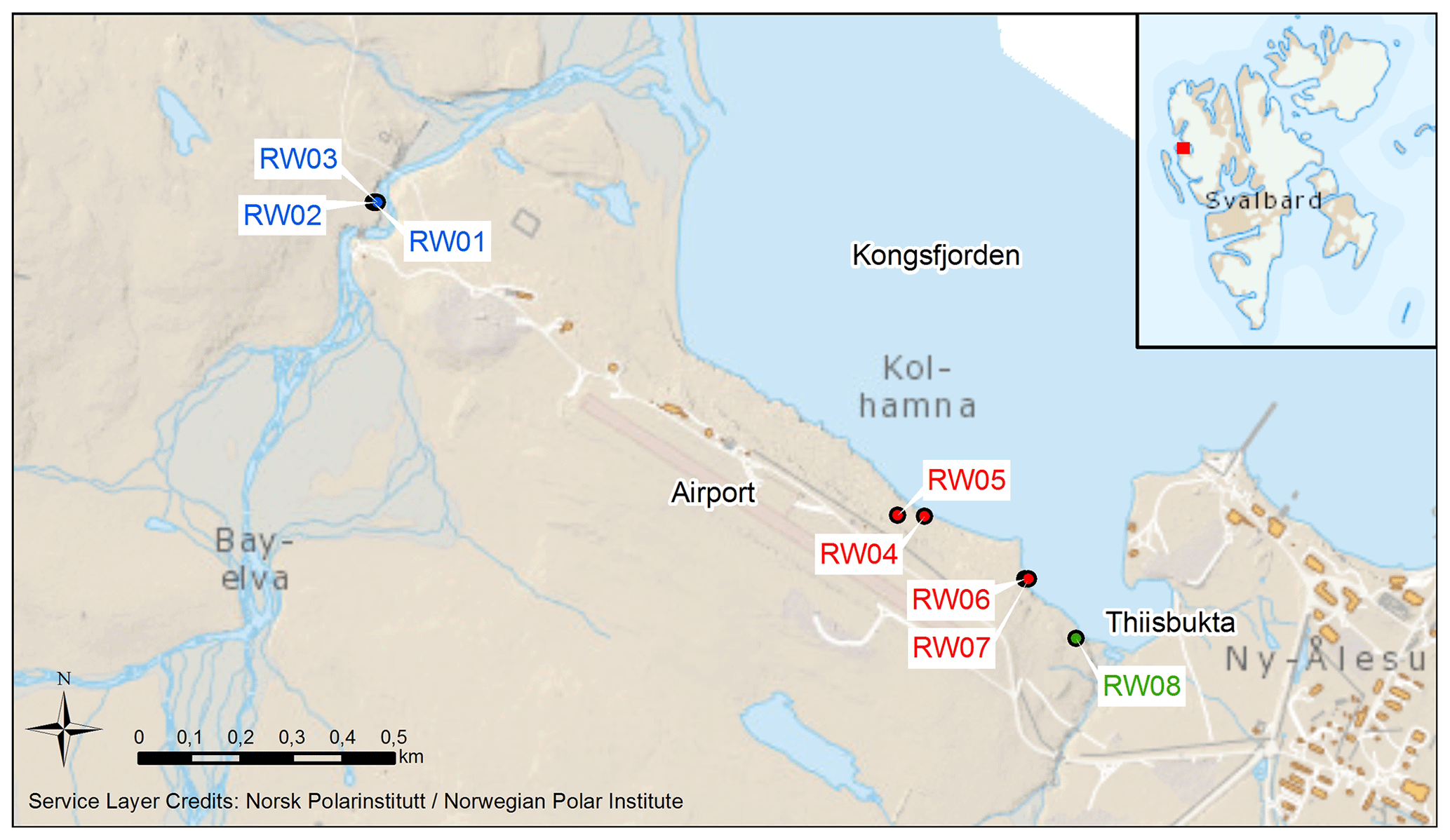
Figure 1 Locations of installed loggers in the canyon (blue labels: RW01 to RW03), at the coastal cliffs (red labels: RW04 to RW07) and in the bay Thiisbukta (green label: RW08). Source: NP_ Basiskart_Svalbard_WMTS_25833/FKB_Svalbard_WMTS_25833, ETRS89 UTM 33 © Norsk Polarinstitutt (https://www.npolar.no/, last access: 7 July 2020).

Svalbard is located in the northern part of the warm North Atlantic current, and therefore, it is very sensitive to atmospheric and oceanic changes (Walczowski and Piechura, 2011). Increasing air temperatures have been observed for more than a century (Nordli et al., 2020). Climate models predict an increase in precipitation and a warming of air temperature with the most pronounced air temperature change in the winter season (Hanssen-Bauer et al., 2019; Isaksen et al., 2016). The climatic changes are also apparent in permafrost temperatures on Svalbard as observed in boreholes over the last few decades (Boike et al., 2018; Christiansen et al., 2010; Etzelmüller et al., 2020; Isaksen et al., 2007). Simulated thermal conditions on Svalbard show an increase in ground temperatures and indicate significant warming and an increase in active layer thickness over the 21st century (Etzelmüller et al., 2011). Besides large-scale climate changes, local conditions can play an important role in the surface energy budget, resulting in an amplification or dampening of the large-scale signal (Westermann et al., 2009). Besides sensible and latent heat fluxes, shortwave and longwave radiation are crucial factors as they have a strong impact on the energy transfer processes from the atmosphere to the ground, effectively modulated in the presence of insulating snow cover (Gisnås et al., 2014, 2016; Haberkorn et al., 2015a, 2017). The terrain exposure induces significant spatial variability in shortwave radiation that should be considered when modeling thermal conditions in inclined slopes (Fiddes and Gruber, 2014; Magnin et al., 2015).

Besides down-welling radiation, longwave radiation emitted by water bodies as well as reflected shortwave radiation on snow and ice can influence the rock surface temperature. Therefore, sea ice coverage plays an important role in the surface energy balance of coastal cliffs. According to observations since 1997, Kongsfjorden used to be characterized by sea ice cover during the winter season (Gerland and Hall, 2006). Since 2006, the sea ice extent has been reduced significantly and the ice thickness and snow cover on ice have become thinner (Johansson et al., 2020). This could also affect coastal erosion as sea ice and development of an ice foot protect the cliffs by absorbing ocean wave energy and control the removal of weathered material from the base of the cliff (Ødegård and Sollid, 1993). With shorter or absent fast-ice periods, coastal cliffs are exposed to waves and tides for longer durations. Climate models predict a further reduction in sea ice cover in the western fjords of Svalbard (Hanssen-Bauer et al., 2019). Thus, thermal models for steep rock walls have to consider the influence of aspect and slope angle on radiative forcing as well as additional heat sources like open seawater and reflection of shortwave radiation on sea ice.

In this study, we applied a full energy balance model to evaluate the role of the different radiative forcing elements in the thermal regime in steep slopes at a high-Arctic site. In doing so, we extended the parametrization of radiative forcing in the thermal model CryoGrid 3 to account for effects governing steep rock walls, and we validated the model with measured rock wall temperatures in the study area. Our objectives were to analyze the effect of coastal and near-coastal settings on (i) rock surface temperatures of vertical rock walls and (ii) the surface energy balance throughout the seasons and (iii) to estimate future developments of the thermal regime until 2100 for these settings.

2 Study site

The observation site is situated near the village of Ny-Ålesund, Kongsfjorden, located on the west coast of Spitsbergen. We measured rock surface temperatures in steep coastal and near-coastal rock walls (Fig. 1). Carbonate rocks of Permian to Carboniferous age with an apparent joint system are the dominant bedrocks (Fig. 2). The surrounding of the study area is a strandflat and is characterized by tundra vegetation, while the surface sediments are dominated by fine- to medium-grained glacial and marine deposits (Hop and Wiencke, 2019; Westermann et al., 2009).

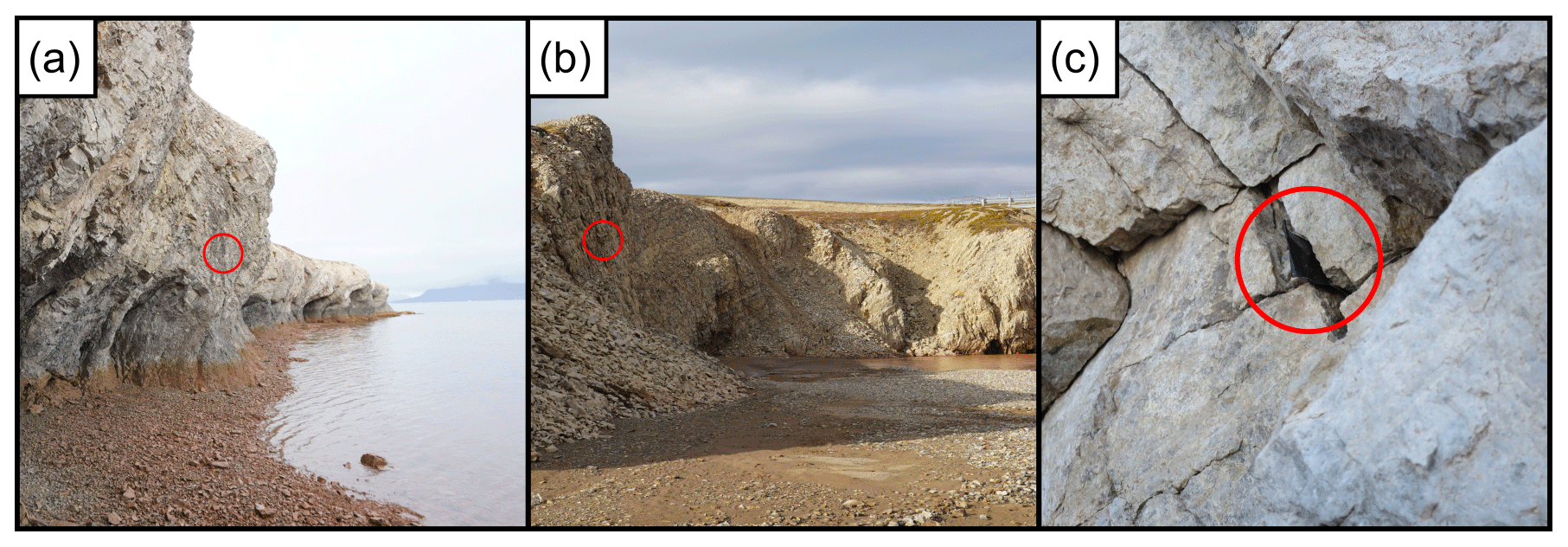
Figure 2 Locations of rock wall loggers used in this study: (a) coastal cliffs at the open fjord next to Ny-Ålesund airport (tidal zone visible at bottom). The position of RW06 is marked with a red circle. (b) Near-coastal rock walls in the canyon of Bayelva. The position of RW01 is marked with a red circle. (c) Close-up of a rock wall logger location: marking tape is visible, while the logger is located about 5 cm inside the crack in thermal contact with the rock.

Long-term records of climatological parameters are evidence of ongoing changes in the Arctic climate system with an increase in mean annual temperature by $+\mathrm{1.3}\pm \mathrm{0.7}$ ^∘C per decade and a rise during winter months by $+\mathrm{3.1}\pm \mathrm{2.6}$ ^∘C per decade. The winter warming is linked to a change in net longwave radiation of $+\mathrm{3.9}\pm \mathrm{3.9}$ W m⁻² per decade (Maturilli et al., 2015). The net shortwave radiation is mainly altered in the summer season by $+\mathrm{12.0}\pm \mathrm{12.0}$ W m⁻² per decade due to the decrease in reflection caused by a reduced snow cover duration (Hop and Wiencke, 2019; Maturilli et al., 2015).

The main surface wind direction is along the axis of Kongsfjorden from the inland to the coast throughout all seasons. The mountains cause complex wind fields (Maturilli and Kayser, 2017), and a southeasterly wind flow occurs as a result of channeled winds from the Kongsvegen glacier (Beine et al., 2001). Measured mean annual precipitation in Ny-Ålesund in the period 2000–2019 was 484 mm (annual precipitation in Svalbard, Hopen and Jan Mayen, filtered; Environmental monitoring of Svalbard and Jan Mayen (MOSJ), 2021). It can occur as both rain and snow throughout the year, but the snow-free season is typically from June to October (Hop and Wiencke, 2019).

3 Methods

3.1 Surface rock temperature monitoring

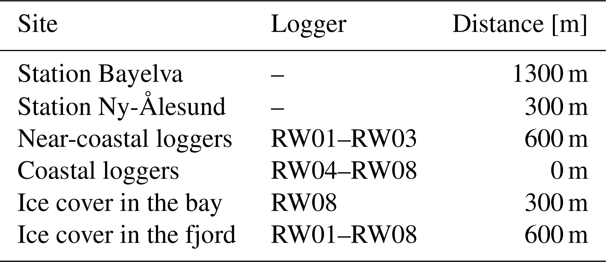
In this study, we used eight iButton (© Maxim) temperature loggers (Table 1) which were installed during the summers and springs of 2016 and 2017 in different locations near Ny-Ålesund in Svalbard. The measurement sites are labeled with RW01 to RW08 (Fig. 1) and are located in near-vertical north- to east-facing rock walls. They represented three different settings: (i) near-coastal rock walls in the canyon of Bayelva (three locations), located about 600 m from the open fjord; (ii) coastal cliffs at the open fjord next to Ny-Ålesund airport (four locations); and (iii) a coastal cliff in the bay of Thiisbukta (one location). The settings allowed the analysis of permafrost temperatures in near-coastal rock walls and coastal cliffs affected by seawater (Fig. 2).

Table 1 Settings of surface temperature loggers used in this study at eight different locations RW01–RW08 in the surroundings of Ny-Ålesund, Svalbard.

The temperature sensors were placed in deep cracks in the rock wall so that both sides of the iButton are in direct thermal contact with the rock surface and the sensor is protected from sunlight (Fig. 2c). The measurement accuracy of iButtons is estimated at 0.5 ^∘C by the manufacturer, and no additional calibration was used. The numerical precision of the sensor readout was set to 0.0625 ^∘C, with a sampling rate of 4 h. At each measurement site, we installed at least one more iButton, generally placed within 10 cm of the main sensor in exactly the same aspect but often in different cracks or different parts of the same crack, to evaluate the uncertainty in the sensor and/or logger system. We used these duplicate measurements to evaluate the combined uncertainty in the sensor and/or logger system and the placement in the walls. For all sites, the differences between the two sensors were found to be less than 0.1 ^∘C for annual averages, while seasonal averages showed differences of less than 0.2 ^∘C.

3.2 Model description

We adapted the CryoGrid 3 ground thermal model (Westermann et al., 2016), originally designed for horizontal surfaces, to account for conditions in steep rock walls (Magnin et al., 2017). CryoGrid 3 calculates rock temperatures by solving the heat equation, uses the surface energy balance as an upper boundary condition and considers latent heat effects depending on water content of the substrate as performed in Westermann et al. (2016). The heat transfer to the ground is calculated by heat conduction. The surface energy balance is derived from time series of air temperature, specific humidity and wind speed at a known height above the ground; incoming shortwave and longwave radiation; air pressure; and rates of snowfall and rainfall (Westermann et al., 2016). In the standard version designed for horizontal surfaces, turbulent fluxes between the surface and the atmosphere are controlled by vertically moving air parcels as defined in the Monin–Obukhov similarity theory (Monin and Obukhov, 1954). As a consequence, movement of air parcels at a vertical wall would be parallel to the surface rather than perpendicular. Therefore, we assumed in all model calculations that the near-surface wind profile follows a neutral atmospheric stratification. To do so, we applied the same approach as Magnin et al. (2017), who used CryoGrid 3 to simulate rock wall and permafrost temperatures at the Aiguille du Midi, France.

Besides the analysis of rock surface temperatures (RSTs), we used CryoGrid 3 to determine the active layer thickness (ALT). We applied a small grid spacing in the upper layers (0.1 m between 0 and 1 m depth) and gradually increased the grid spacing to the lower layers of the model (10 m between 50 and 100 m depth) to account for detailed ground temperature calculations in the active layer near the surface.

We define the surface as the interface between the atmosphere and the rock wall. Fluxes, which transport energy away from the surface, have a negative sign, while fluxes, which transport energy towards the surface, are denoted positive.

3.3 Preprocessing

As the energy input of shortwave and longwave radiation depends on varying aspects and slope angles of the rock walls, we modified the model to account for the different physical settings of the logger locations. We calculate incoming shortwave radiation as the sum of direct, diffuse and reflected shortwave radiation, while incoming longwave radiation includes atmospheric longwave radiation as well as heat emission of the close environment.

We divided shortwave radiation into direct and diffuse components (Fiddes and Gruber, 2014). This required the determination of the atmospheric clearness index k_t, the ratio between solar radiation arriving at the surface S_in and the radiation at the top of the atmosphere S_TOA:

$$\begin{array}{}\text{(1)}& k_{\mathrm{t}}={\displaystyle \frac{S_{\text{in}}}{S_{\text{TOA}}}}.\end{array}$$

The fraction of diffuse shortwave radiation k_d was computed based on the clearness index k_t,

$$\begin{array}{}\text{(2)}& k_{\mathrm{d}}=\mathrm{0.952}-\mathrm{1.041}{e}^{-\exp (\mathrm{2.300}-\mathrm{4.702}\cdot k_{\mathrm{t}})},\end{array}$$

taking into account the sky view factor SVF. As we applied the model to vertical rock walls, we assumed an SVF of 0.5 for all locations (Kastendeuch, 2013). Therefore, the amount of diffuse shortwave radiation S_diff can be expressed as

$$\begin{array}{}\text{(3)}& S_{\text{diff}}=\text{SVF}\cdot k_{\mathrm{d}}\cdot S_{\text{in}}.\end{array}$$

Consequently, the amount of direct shortwave radiation S_dir is the remaining fraction $(\mathrm{1}-k_{\mathrm{d}})\cdot S_{\text{in}}$. After we determined the azimuth α_sun and elevation β_sun of the sun for every time step depending on latitude, longitude and altitude of each location, we projected direct shortwave radiation S_dir on inclined slopes (Appendix A).

Besides direct and diffuse shortwave radiation, we implemented reflected shortwave radiation in the model to account for diffuse reflection on ice and snow surfaces as well as on snow-free terrain. Assuming Lambertian reflectance, we derived reflected shortwave radiation S_ref, taking into account the albedo of the surface α and the sky view factor SVF:

$$\begin{array}{}\text{(4)}& S_{\text{ref}}=S_{\text{in}}\cdot \mathit{\alpha }\cdot (\mathrm{1}-\text{SVF}).\end{array}$$

We used the sum of diffuse, direct and reflected shortwave radiation as a driving variable for the model CryoGrid 3 on vertical rock walls.

Moreover, we modified longwave radiation by using the implemented sky view factor SVF. For simplicity, we assumed an SVF of 0.5 for all locations, so 50 % of the longwave radiation is given by the forcing data L_{in_forc}, representing the atmospheric longwave radiation, while the rest is derived from the ambient temperature T_amb applying the Stefan–Boltzmann law with the Stefan–Boltzmann constant σ (Fiddes and Gruber, 2014):

$$\begin{array}{}\text{(5)}& L_{\text{in}}=\text{SVF}\cdot L_{\text{in}\mathit{\_}\text{forc}}+\left(\mathrm{1}-\text{SVF}\right)\cdot \mathit{\sigma }\cdot {\left(T_{\text{amb}}+\mathrm{273.15}\right)}^{\mathrm{4}}.\end{array}$$

With this approach, we assumed that incoming longwave radiation is isotropic. The ambient temperature T_amb was given by either the air temperature or the sea surface temperature in the case when the logger was located directly above the sea. If the seawater was covered by ice and could not emit any heat, we used air temperature for deriving the longwave radiation.

Apart from the modification of incoming shortwave and longwave radiation, we included the water balance in the model by implementing a water bucket approach. Due to the vertical alignment of the rock walls and the consistency of hard bedrock, precipitation did not infiltrate into the material and evaporation of moisture at the rock surface dominated the latent heat flux. Therefore, the latent heat flux had only a minor influence on the total surface energy balance and a simplistic water bucket approach was sufficient for the required model setup (Appendix B).

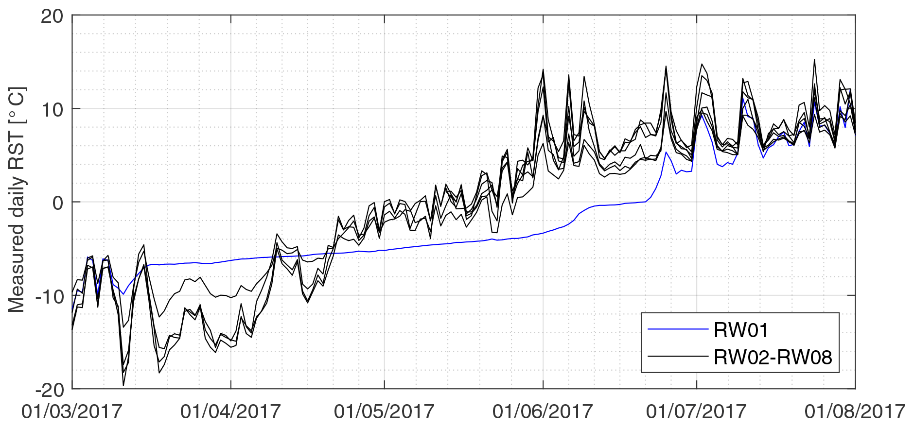
Figure 3 Mean measured daily RST in winter 2017. RW01 shows a temporarily damped signal due to snow cover.

We did not consider snow cover in the model, which was adequate for most of the measurement data in the analyzed time period from 2016 to 2020. An exception is displayed in Fig. 3, showing the damped signal of RW01 due to snow cover. Besides spring 2017, RW01 was influenced by snow over a period of 2 to 3 months in spring 2019 and 2020. In the other measurement sites, snow cover was only briefly observed in May 2019 (RW05) and in May 2020 (RW05, RW06, RW08). Further evaluations on the possible influence of snow cover are given in the Supplement, where we present model runs considering snow cover in the rock walls following the model approach of Magnin et al. (2017).

3.4 Model parameters and forcing data

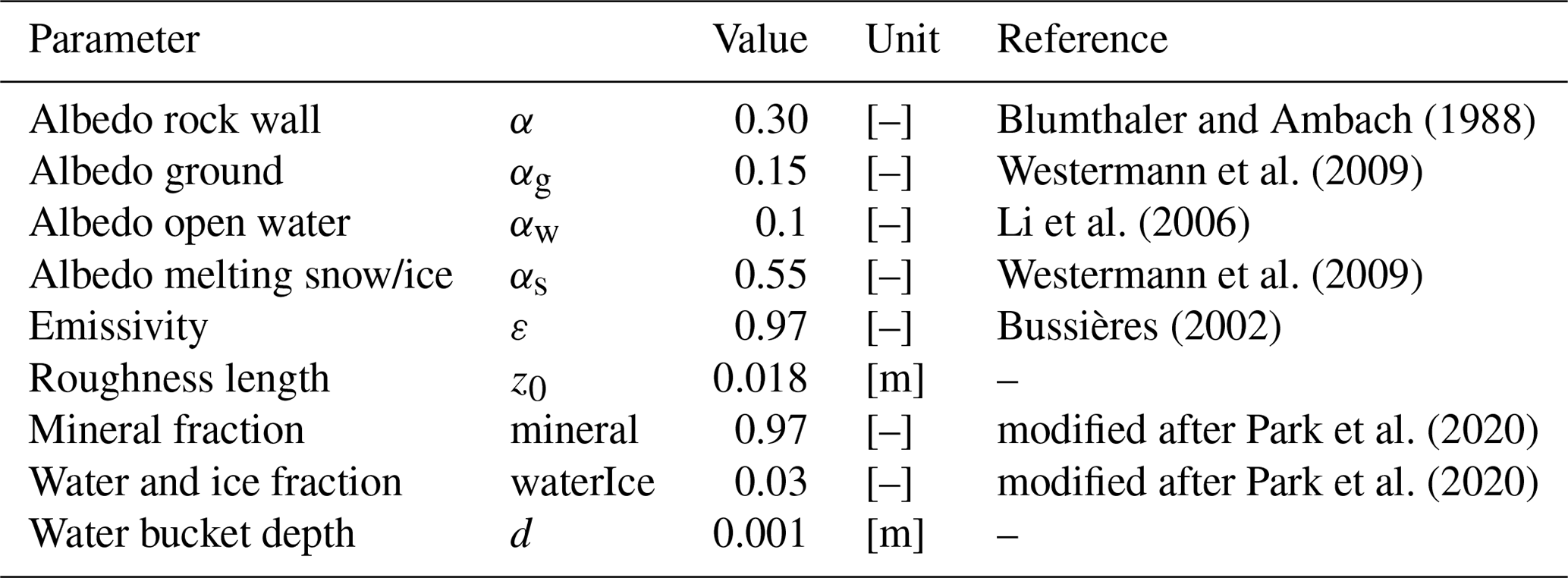
The study focused on rock surface temperatures; thus simplified subsurface properties were implemented (Table 2). We considered the bedrock to have a volumetric mineral content of 97 % and a volumetric water content of 3 %, which implied saturated conditions during the entire simulation. The assumed porosity was selected to be higher than measurements of 0.5 % of fresh carbonate samples without cracks in the Ny-Ålesund region (Park et al., 2020), with the goal to account for the fractured nature of the rock walls. Due to the high uncertainty in this value, a sensitivity study was performed for the volumetric mineral and water content. The albedo for limestones was found to be between approximately 0.22 and 0.32 (Blumthaler and Ambach, 1988), and as light-colored carbonates build up the cliffs, we assumed an albedo of 0.3 in the model setup. An important fitting parameter was the roughness length z₀ as performed in Magnin et al. (2017). We set it to a value of 0.018 m, which represents roughly $\mathrm{1}/\mathrm{10}$ of the height of the surface roughness elements. This fitted well to the small-scale variations on the rugged rock surface characterized by joint systems (Fig. 2), but uncertainties regarding the different spatial scale of roughness elements in the rock walls remain. We set the albedo for the horizontal ground surface to 0.15 (Westermann et al., 2009) and for water surfaces to 0.1, which is in the range of the surface ocean albedo for the typical high solar zenith angles on Svalbard (Li et al., 2006; Robertson et al., 2006). The albedo for ice and snow was set to a relatively low value of 0.55, as the highest influence of reflected shortwave radiation was expected for spring, when snowmelt decreases the albedo. This is in line with the reported decrease in albedo from 0.8 to 0.5 in Westermann et al. (2009). All values can be found in Table 2, and a sensitivity study for selected parameters is provided in the Supplement.

Table 2 Model parameters assumed in the simulations.

Atmospheric forcing was provided by the AROME-Arctic weather model, which is a regional, high-resolution, non-hydrostatic, numerical weather prediction system for the European Arctic (Müller et al., 2017). It is based on HARMONIE-AROME as part of the ALADIN-HIRLAM system, which provides short-range weather forecasts for northern and southern European countries (Bengtsson et al., 2017; Seity et al., 2011). Archive files of atmospheric data since October 2015 are available. In 2017, updates were implemented to improve high-resolution weather forecasts over the Nordic regions (Müller et al., 2017). AROME-Arctic operates on a resolution of ∼2.5 km grid spacing at 65 vertical levels. We used time series ranging from October 2015 to August 2020 from AROME-Arctic as forcing data for the model. The nearest 2.5 km grid cell of AROME-Arctic to the required locations was located northeast of Ny-Ålesund in Kongsfjorden (78.9^∘ N, 11.98^∘ E; 20 m a.s.l.). The selected grid cell covers both parts of the fjord and the adjacent land surface and therefore provides suitable forcing data for the loggers located directly at or within a short distance of the shoreline. The driving variables absolute humidity, wind speed, down-welling shortwave and longwave radiation, air pressure, and rates of snowfall and rainfall for this grid cell have been extracted from the archive. Incident solar radiation at the top of the atmosphere was provided by ERA5 (Hersbach, 2016).

The spatial resolution of air temperature given by AROME-Arctic was not sufficient to capture small-scale variabilities. Therefore, we used records from two climate stations to force the model (Boike et al., 2018, 2019; Maturilli, 2020a–i; Boike et al., 2021). The Baseline Surface Radiation Network (BSRN) station in Ny-Ålesund is located in the village center (78.9250^∘ N, 11.9300^∘ E) with a distance of about 300 m to the coast (Maturilli et al., 2013). The second station at the Bayelva site is located on top of the Leirhaugen hill, which is within a 1.3 km distance of the coast (Boike et al., 2018). Using records of two different stations allowed us to estimate gradients in air temperatures from the coast to environments further inland. For simplicity, we interpolated linearly between the two stations and estimated the air temperature at the rock walls subject to their distance to the open water body of the fjord. As sea ice coverage enlarges the distance to the open water body, we added an additional mean distance (Table 3), estimated by analysis of the web camera time series from the mountain Zeppelinfjellet (Pedersen, 2013).

Table 3 Distances to the open water body used for the linear interpolation of air temperature and logger locations that the distances are applied to.

We used the water temperature of Kongsfjorden recorded by the AWIPEV underwater observatory at a 12 m depth to estimate the longwave heat emission of the water body. The data provide a time series of water temperatures for the entire period from October 2015 to August 2020 with a resolution of 1 h (Fischer et al., 2018a–c, 2019, 2021a, b).

We simulated long-term climate impacts of three different representative concentration pathways (RCPs) RCP2.6, RCP4.5 and RCP8.5 (van Vuuren et al., 2011) for coastal and near-coastal settings. For the period 1980 to 2019, we used forcing data of the ERA-Interim reanalysis, while the years 2020 to 2100 were created using an anomaly approach based on CMIP5 projections of the Community Climate System Model (CCSM4) (CLM4.0 Offline Model Forcing Data Archived from CCSM4 historical and RCP simulations, 2020). Therefore, decadal monthly anomalies were derived from the CCSM4 projections using a reference period from 2009 to 2019 which were then applied to the reanalysis data of the same period (see Koven et al., 2015).

To account for small-scale variabilities between coastal and near-coastal rock walls, we calculated a linear regression using the AROME forcing data. Others parameters were simplified due to a lack of information: sea temperature was set to a constant value of 2.53 ^∘C, which is the mean sea temperature of the analyzed period of 2016 to 2020. Sea ice was assumed in the months February to May until the year 2005 (Gerland and Hall, 2006). Despite these uncertainties, these steps allowed us to analyze possible trajectories for the future developments of the rock wall thermal regime.

3.5 Model scenarios

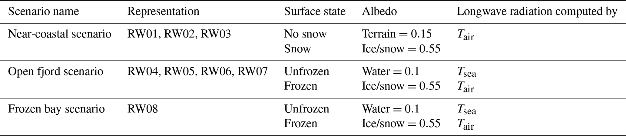
In this study, we considered several scenarios to represent the thermal conditions at the selected rock walls (Table 4). We varied the source of forcing air temperature, the source for heat emission and the albedo of the foot of the slope to account for the different locations. The near-coastal scenario was controlled by conditions either with or without snow at the foot of the slope resulting in temporarily changing albedos for snow and terrain. The frozen bay scenario showed temporarily frozen seawater leading to changes in the source of heat emission and albedo of the foot of the slope. The open fjord scenario was characterized by a predominantly unfrozen fjord during the entire year and had consequently no varying parameters in most of the simulation time. Short periods of a frozen layer occur temporarily so that the model parameters were modified the same way as in the frozen bay scenario. Daily frozen conditions were estimated by analyzing a web camera time series from the mountain Zeppelinfjellet, which provides photos of Ny-Ålesund and the adjacent coastline every 10 min (Pedersen, 2013).

Table 4 Model scenarios and corresponding settings with the three varying parameters source for air temperature: source for longwave heat emission and albedo of the foot of the slope.

4 Results

4.1 Measurements of rock surface temperatures

Mean annual temperatures (September–August) as well as mean temperatures in the winter season (December–February) are given in Table 5. For the measurement period 2016 to 2020, all loggers record below-freezing mean annual rock surface temperatures (MARSTs) with values between −0.6 (RW06 in 2017/18) and −4.3 ^∘C (RW02 in 2019/20). The MARSTs typically vary by up to several degrees between the recorded years, with 2017/18 being the warmest year. Measurements in 2019/20 show the lowest MARST, which is related to a comparatively cold winter (December–February) and spring (March–May) season (Table 5).

Table 5 Measured MARST and mean RST in the winter season (December–February) for all locations RW01 to RW08. Lack of data results from either (¹) snow cover on the logger or (²) missing records. MARSTs are coldest in near-coastal settings (RW01–RW03). Mean RSTs in the winter season are found to be coldest in near-coastal settings, closely followed by settings in the bay (RW08), while settings at the open fjord show the highest RSTs (RW04–RW07).

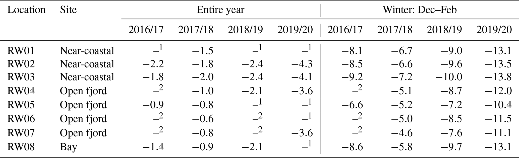
Minimum and maximum daily RSTs are found between −24.2 (RW03) and 18.9 ^∘C (RW06). The variability in daily RST shows a higher frequency in summer and higher amplitudes in winter. Fluctuations in RST are especially pronounced for near-coastal rock walls during the cold periods of the year, while the signal at coastal cliffs at the open fjord is dampened in the same time.

We emphasize that loggers at the coastal cliffs record higher MARST than loggers in near-coastal rock walls with a mean difference in MARST of 1.0 ^∘C (Table 5), although the loggers are located within just about a 1.5 km distance (Fig. 1) at similar elevations. The setting is especially important in winter and spring seasons, and RST differences account for 1.5 to 2.2 ^∘C in these time periods. The lower the temperatures, the larger the temperature difference between these two settings, which is apparent in Fig. 4a.

Besides these observations of RST, time series of station data show that higher air temperatures are recorded for the BSRN station in Ny-Ålesund compared to for the Bayelva site further inland. During the year 2017/18, the air temperature difference was 0.9 ^∘C with the highest differences of 1.6 ^∘C during the winter season and 1.5 ^∘C during the spring season.

We highlight that RST values in the Thiisbukta bay are significantly lower in winter than RST at the coastal cliffs even though the loggers are all located at the shoreline. This is especially true for periods when the bay is characterized by an ice layer on the water (Fig. 4a) but can also be observed for unfrozen conditions in the bay. If not only the bay is frozen but also widespread sea ice occurs in the fjord, RST values in all three settings show about the same temperatures (Fig. 4b).

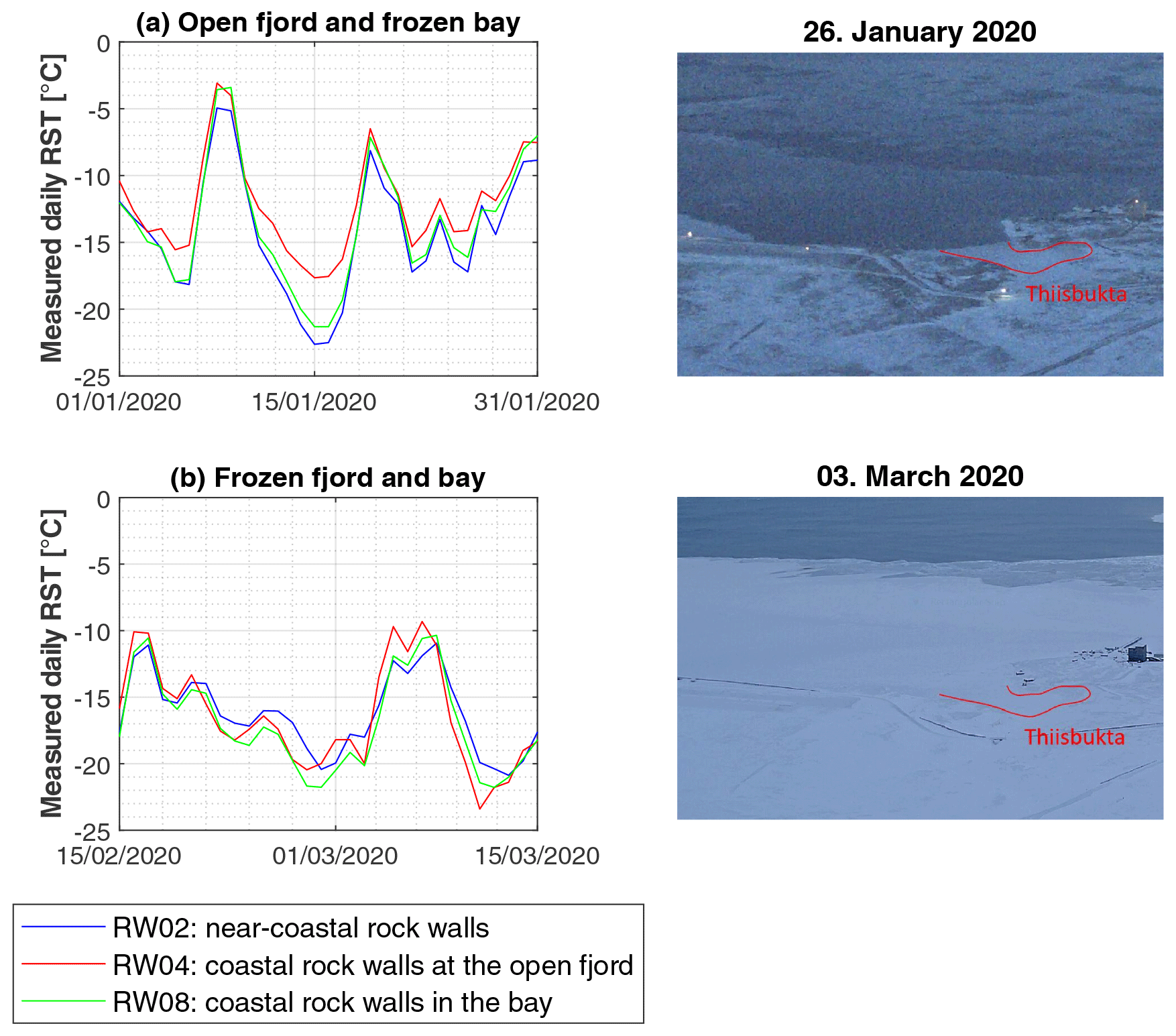
Figure 4 Mean measured daily RST for two different conditions in Kongsfjorden: (a) the time period 1–31 January 2020 was mainly characterized by a frozen bay and an open fjord. RSTs at coastal cliffs show higher values than RSTs at the near-coastal rock walls and at rock walls in the bay. The most pronounced differences are found with RSTs below −10 ^∘C. (b) In the time period 15 February–15 March 2020, the bay and the fjord were predominantly frozen. In this case, no clear differences could be observed between the three settings. RW02, RW04 and RW08 were selected as they have the same aspect but different settings.

4.2 Model validation

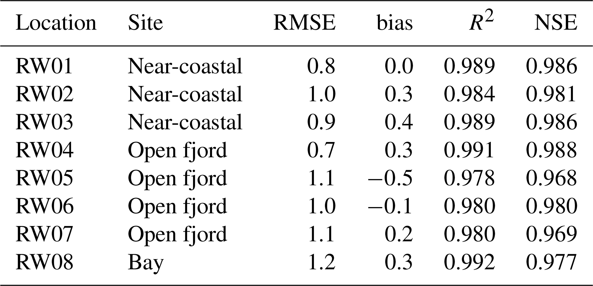
We compared monthly average values of measured rock surface temperature RST to the model results of the near-coastal scenario (RW01, RW02, RW03), the open fjord scenario (RW04, RW05, RW06, RW07) and the frozen bay scenario (RW08). The measured RST was reproduced closely with the applied model setup, especially for temperatures near the freezing point (Fig. 5). Besides the visually good agreement of Fig. 5, a root-mean-square error (RMSE) below 1.2 ^∘C, the bias (−0.5 to 0.4 ^∘C), the coefficient of determination R² (above 0.97) and the Nash–Sutcliffe efficiency NSE (above 0.96) for all locations confirmed a good reproduction of the measured data (Table 6).

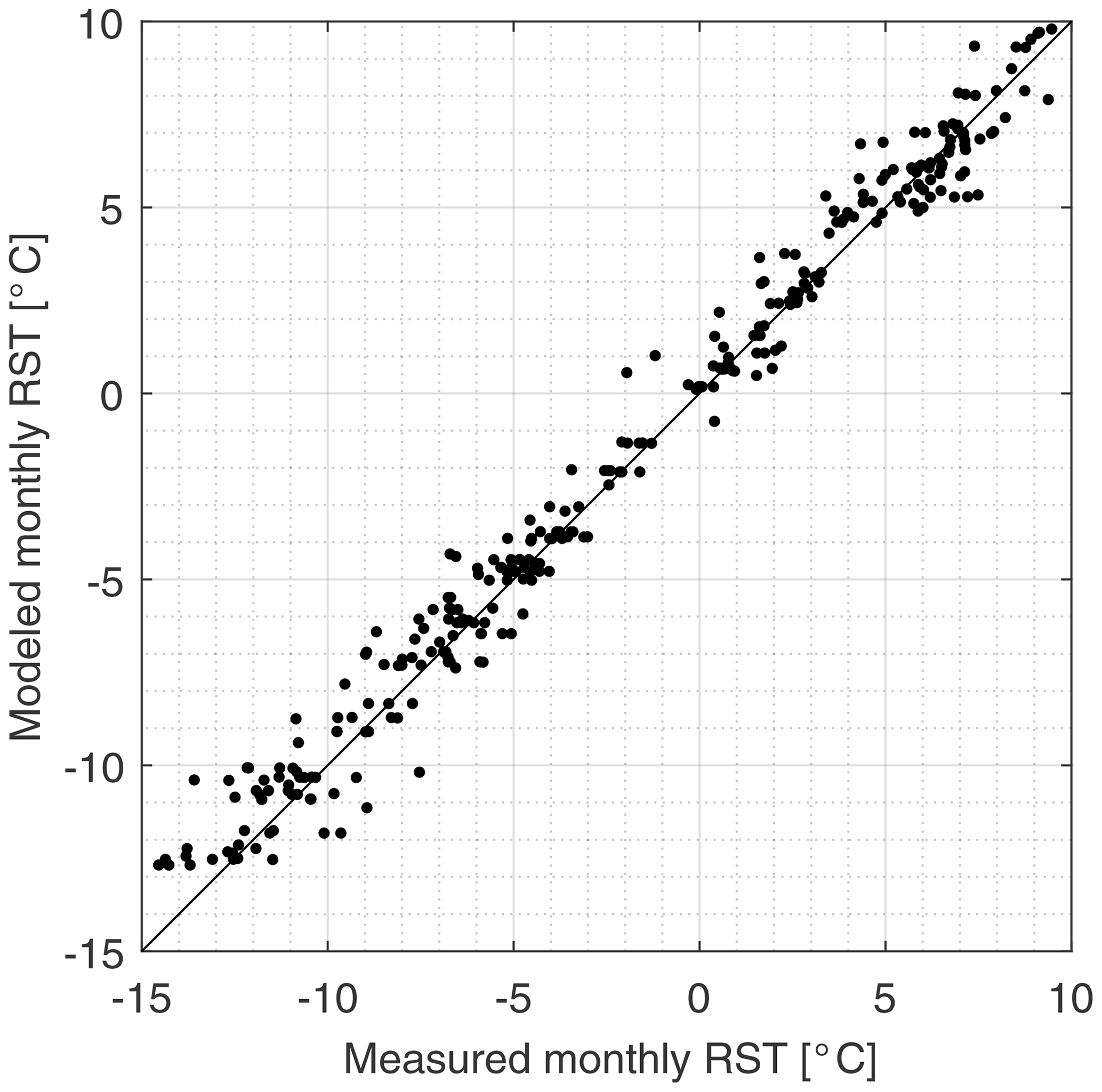
Figure 5 Mean modeled vs. measured monthly RST for all locations RW01 to RW08, comprising each entirely recorded month for the measurement periods stated in Table 1.

Table 6 Summary statistics of the model validation including RMSE, bias, R² and NSE. The statistics were calculated for all locations RW01 to RW08, comprising each entirely recorded month for the measurement periods stated in Table 1.

4.3 The influence of open water and sea ice on RST

The model results are in good agreement with the in situ measurements and corroborate the pattern of open water and sea ice influence on RST.

Below-freezing MARSTs are modeled for all locations, ranging from −0.3 (RW06 in 2017/18) to −3.9 ^∘C (RW02 in 2019/20) with the warmest year being 2017/18 and the coldest year being 2019/20. The lowest MARSTs are modeled at rock walls in the near-coastal scenario, while the open fjord scenario produces the highest MARST.

The model results show differences in MARST according to the exposition of the rock wall: in the open fjord scenario, the lowest MARST in 2017/18 is found on the north-facing rock wall RW05 (−0.9 ^∘C), while the highest MARST is calculated for RW06 facing east-northeast (−0.3 ^∘C). Model runs for north- and south-facing rock walls suggest that differences in MARST due to exposition are only 0.7 ^∘C or less. While no effect is detectable in winter, higher RST variations of up to 1.6 ^∘C are calculated for the spring season.

Simulations with snowfall provided by the forcing data cannot represent the temporarily occurring snow cover in the rock walls adequately. A distinct overestimation of snow cover in early winter and a clear underestimation in late spring result in significant deviations from the measured data. Results of simulations including snow cover are provided in the Supplement.

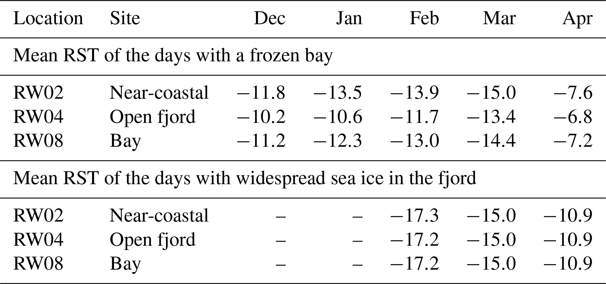
In the model results, we find that temporarily occurring ice cover on the fjord results in lower RST at the nearby rock walls. For time periods with a frozen bay but no sea ice in the open fjord, only RW08 is affected. Model results show a ca. 1–1.5 ^∘C colder RST compared to the other rock walls at the shoreline, but they are still warmer than the modeled RST in near-coastal settings. However, the results indicate that days with a widespread sea ice extent in the fjord lead to similar RSTs in all locations (Table 7).

Table 7 Modeled mean RST with frozen conditions in the bay or sea ice in the fjord. Frozen conditions in the bay lead to a local cooling of RW08, while sea ice results in similar RSTs for all settings. RW02, RW04 and RW08 were selected as they have the same aspect but different settings.

Lower RST values under frozen conditions can be traced back to three different factors: while (1) lower air temperature and (2) the lack of heat emission from the ocean lead to a cooling of RST, (3) the reflection of shortwave radiation on the ice layer increases RST as an additional energy source. The amount to which these factors influence the decrease in RST between the open fjord scenario and the frozen bay scenario is given in Fig. 6. Between December and February, air temperature and the lack of radiative heating are the dominant factors, while reflected shortwave radiation plays no role. In March and April, the influence of reflected shortwave radiation increases as polar night conditions end. As no sea ice occurred after April in the measurement period 2016 to 2020, no analysis could be performed for the late spring and early summer season.

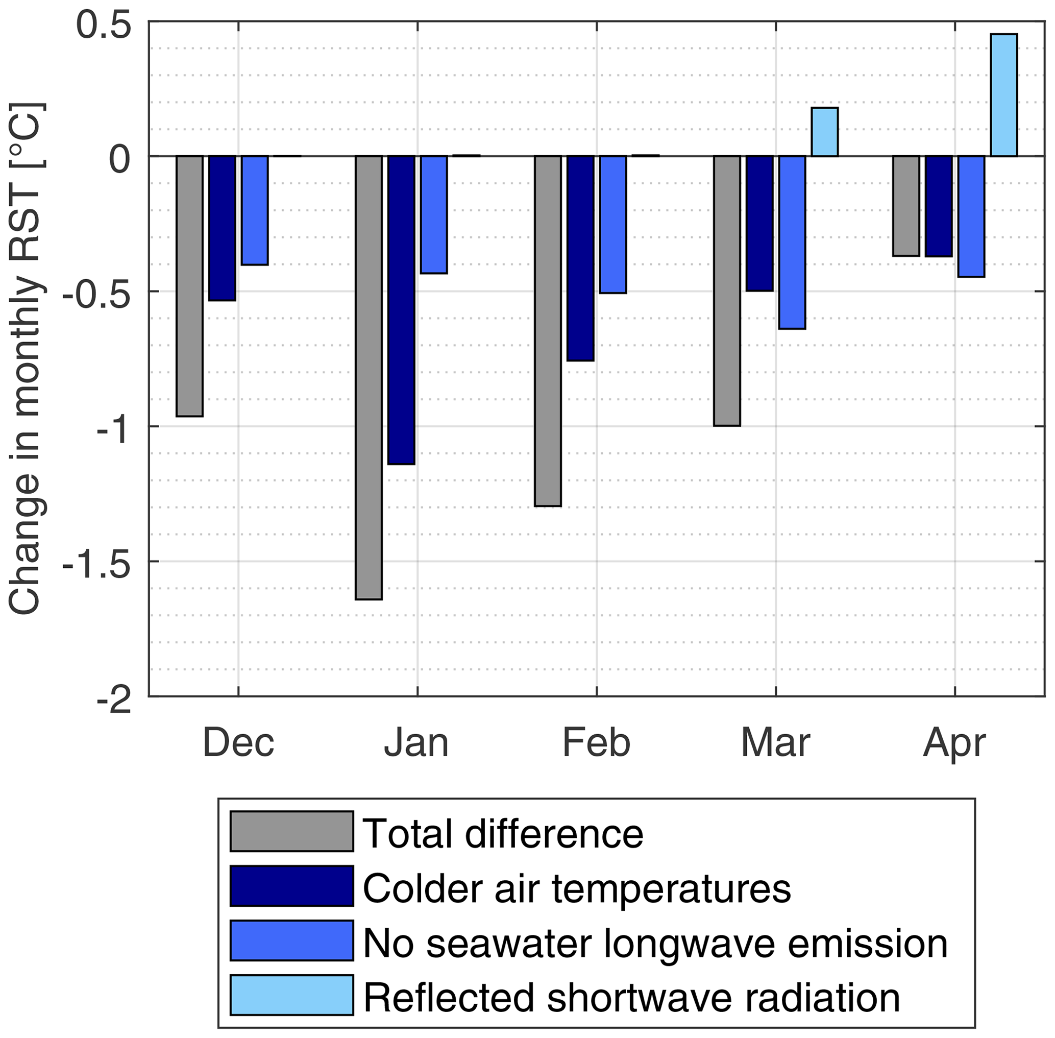
Figure 6 Temperature difference between the open fjord scenario (reference) and different model scenarios. Colder air temperatures: same as reference but using colder air temperature as distance to the open water body is enlarged. No seawater longwave emission: same as reference but using air temperature instead of seawater temperature. Reflected shortwave radiation: same as reference but assuming ice albedo for the surrounding terrain. Total difference: frozen bay scenario combining all three effects.

4.4 The surface energy balance

Individual fluxes of the surface energy budget in the different seasons are given in Fig. 7 (winter is December–February; spring is March–May; summer is June–August; fall is September–November) with positive fluxes directed towards the surface. For comparison of the different scenarios, the fluxes are calculated for vertical rock walls with an aspect of 40^∘ (∼NE), which comprises model runs of RW02, RW04 and RW08.

Figure 7 Surface energy balance for the seasons of the year for a vertical rock wall with an aspect of 40^∘ (RW02, RW04 and RW08). The most pronounced differences in the scenarios are found in winter and spring, while summer and fall show similar fluxes. SW is net shortwave radiation; LW is net longwave radiation; Qe is latent heat flux; Qh is sensible heat flux; G is ground heat flux.

During winter which mostly coincides with polar night conditions (25 October to 14 February), shortwave radiation is zero or only reaches very small values. During this period, the system loses energy mainly due to negative net longwave radiation, which is especially pronounced for the near-coastal scenario, followed by the frozen bay scenario. The loss of energy is opposed by positive sensible heat fluxes, representing a warming of the surface and a cooling of the atmosphere. Strong sensible heat fluxes are associated with high wind speeds and high temperature differences between air and rock wall. Compared to the other terms of the surface energy balance, the negative ground heat flux leading to ground cooling is only small.

In spring, net shortwave radiation increases significantly and becomes the dominant energy source with the highest energy input for the near-coastal scenario and the lowest for the open fjord scenario. Longwave radiation counteracts this process and cools the surface with the highest fluxes in the near-coastal scenario. Besides, sensible heat fluxes contribute to the energy loss with slight differences in the scenarios. However, sensible heat fluxes and emitted longwave radiation cannot compensate for the incoming energy by shortwave radiation and RST as well as ground heat fluxes starting to increase, especially as no energy is used for melting due to snow-free conditions.

The summer period is characterized by similar fluxes in the surface energy balance in all scenarios. The warming of RST continues due to strong shortwave radiation as the main energy source. Energy is lost by longwave radiation and sensible heat fluxes, but latent heat fluxes also cool the surface. However, these fluxes cannot compensate for the energy input. Consequently, the ground heat flux increases even more, leading to seasonal thawing of the active layer.

During fall, net shortwave radiation decreases rapidly due to shorter days, but sensible heat fluxes turn positive, acting as an energy source again. The loss of energy by longwave radiation is slightly higher for near-coastal scenarios and ground heat fluxes are close to zero, indicating the turn to refreezing of the active layer.

In the course of a year, shortwave radiation is naturally the main source of energy to the system, while most energy is lost by longwave radiation. Sensible heat fluxes warm the surface in fall and winter, while they cool in spring and summer. Latent heat fluxes are of minor importance, reflecting the small water-holding capacity of the rock surface assumed in the model. Net ground heat fluxes are close to zero.

4.5 Simulations of future climate change scenarios

The past and future simulations of different RCPs show an increase in MARST for both the near-coastal and the open fjord scenario (Fig. 8). Between 1980 and 2020, MARST increases by several degrees and the MARST difference of the near-coastal scenario and the open fjord scenario is significant. We emphasize that in this period winter sea ice loss has been drastic in Kongsfjorden, going from a normally frozen fjord to a normally open fjord. Thus, in reality, the actual warming may have even been higher than either of the scenarios suggest. Figure 8 clarifies that the current measurement period represents relatively warm years in the occurring fluctuations in MARST and a drop to colder MARST in 2020.

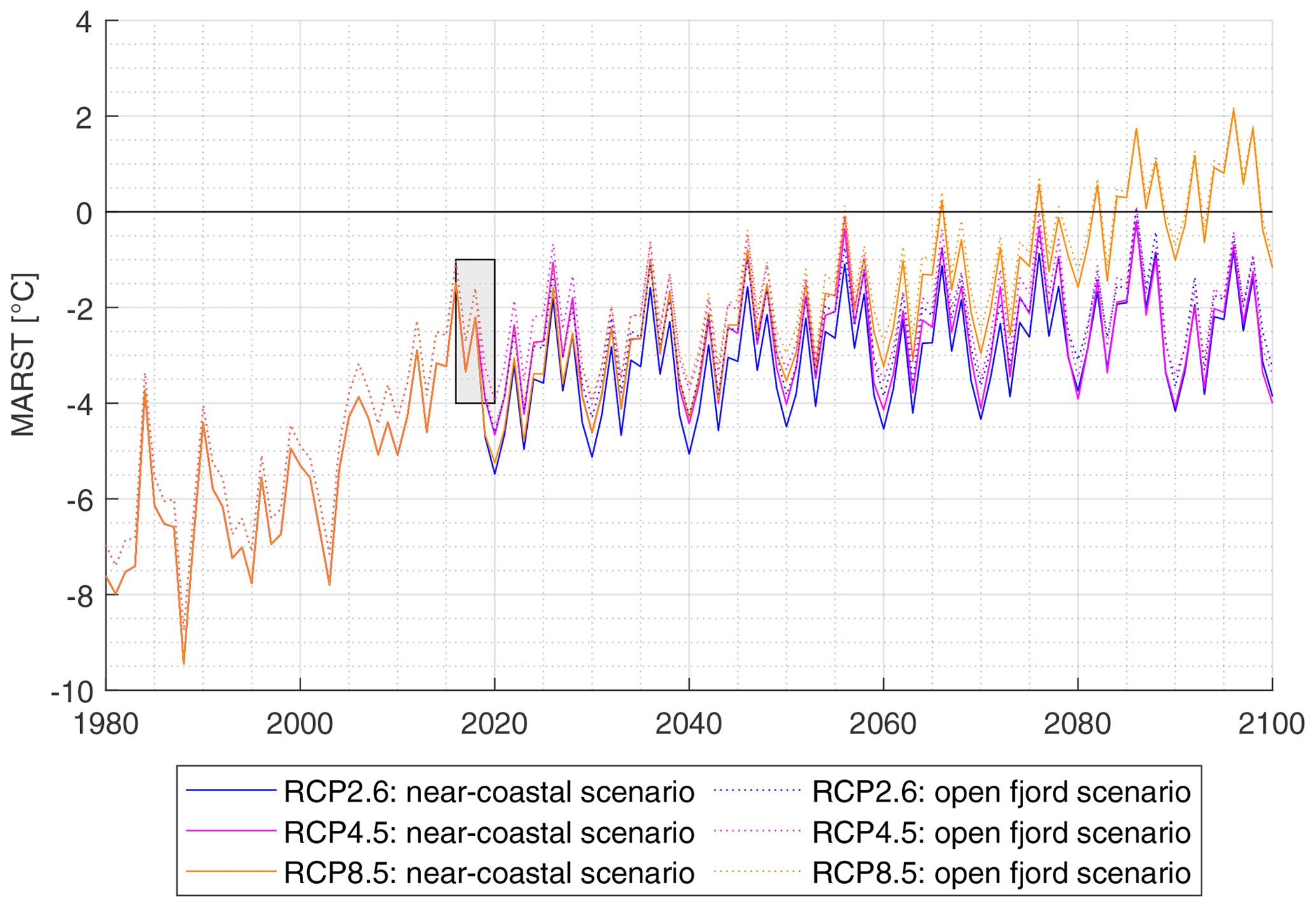
Figure 8 MARST of past and future simulations with the settings of the near-coastal scenario and the open fjord scenario with RCP2.6, RCP4.5 and RCP8.5. The grey box shows the measurement period.

During the years 2020 to 2080, all three pathways show slightly increasing MARST. The influence of the different rock wall locations decreases with time, and consequently, MARST values of the near-coastal and open fjord scenario become more aligned. After 2080, RCP2.6 and RCP4.5 are stabilized with MARST between −4 and 0 ^∘C, while RCP8.5 shows further increasing MARST reaching mean annual values of up to 2 ^∘C.

The model results suggest that a large part of the warming in RST has already happened by the year 2020, while the prospective increase in RST in the 21st century will bring the permafrost close to thawing.

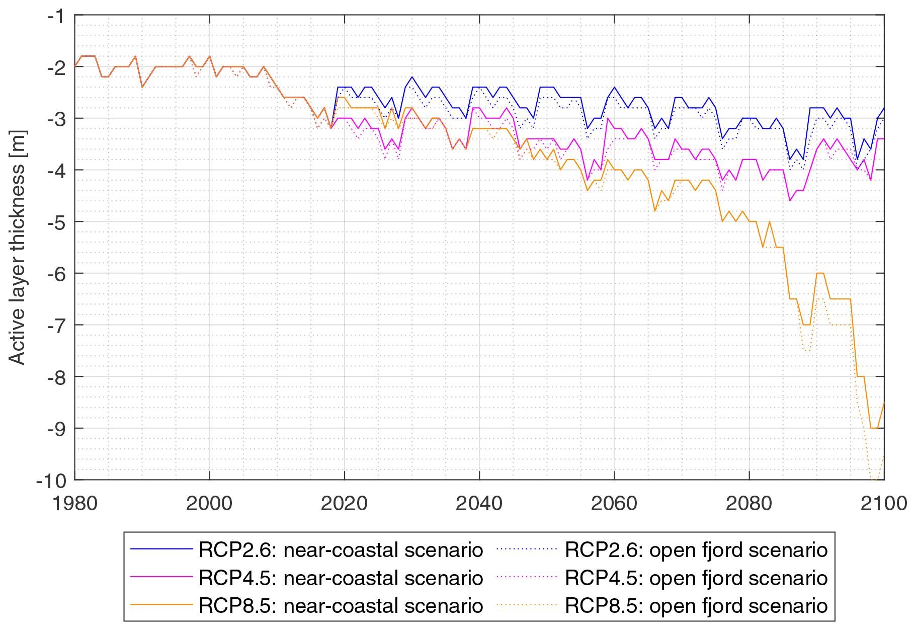
Figure 9 Active layer thickness of past and future simulations with the settings of the near-coastal scenario and the open fjord scenario with RCP2.6, RCP4.5 and RCP8.5.

Furthermore, simulations of the RCPs suggest an effect on the active layer thickness ALT (Fig. 9). Between 1980 and 2010, ALT is about 2 m, with a slightly deeper active layer for the open fjord scenario. After 2010, the ground begins to thaw deeper during the summer season, but the future evolution varies between the three simulated RCPs: RCP2.6 is characterized by a slight increase in ALT and a stabilization between 2.5 and 3.5 m after 2080. RCP4.5 shows a similar trend with ALT between 3.0 and 4.5 m at the end of the century. However, the simulation of RCP8.5 results in a significant increase in ALT below 8 m and with no apparent stabilization effect. Moreover, a talik develops after 2095, implying that the cold winter seasons do not lead to a freezing of the entire ground column anymore.

5 Discussion

5.1 Measurement and model uncertainties

To measure rock surface temperatures, we employed simple iButton temperature loggers, which feature a measurement accuracy of 0.5 ^∘C. While they were not additionally calibrated prior to deployment, we installed duplicates to quantify the combined uncertainty in the sensor and/or logger system and the placement in the rock walls. For all sites, the long-term temperature differences between the two sensors (see Sect. 3.1) were found to be significantly smaller than the differences in MARST between different rock wall sites, which the key results of this study are based on. We therefore conclude that our findings are well supported in the light of the measurement uncertainty.

Our model setup contains uncertainties regarding unknown model parameters, which were estimated using the literature and calibrating the model. Especially rock (surface) parameters could be improved by a more precise analysis of the lithological characteristics.

A critical point is the assumption of a neutral atmospheric stratification perpendicular to the vertical rock wall, which must be regarded as a first-order approximation as it does not account for the complex wind field and boundary layer conditions near the rock wall. This leads to uncertainties in near-surface turbulent exchange of the vertical wall as micro-topography and changing weather conditions can influence the movement of the air parcels. Wind profiles perpendicular to the wall as well as measurements of air temperature and humidity could help to estimate the importance of this error source. However, we scaled the roughness length z₀ to compensate for these assumptions and to fit the modeled surface temperatures to the observed values.

Another error source is the estimation of air temperature at the logger location. The linear interpolation between the two stations and the dependency on the distance to the open water body of the fjord comprise a coarse approximation at best which does not take the wind direction, the atmospheric boundary layer structure and the local micro-climate into account. Air temperature measurements at the shoreline could help to improve the quality of the forcing data.

5.2 The influence of open water and sea ice on RST

In the time period 2016 to 2020, all records display negative MARST, which indicates permafrost conditions at all locations (Table 5). Svalbard lies in the continuous permafrost zone (Brown et al., 1997; Obu et al., 2019), and deep permafrost is observed in the area, e.g., within the abandoned mine shafts (Liestøl, 1977) and in boreholes (Christiansen et al., 2010). We found that the exposition of the rock wall only leads to small differences in MARST. In the winter season, polar night conditions suppress any dependence on exposition, while the effect is most pronounced in the spring season for low sun angles. In general, the influence of exposition in the high Arctic is small compared to at sites at lower latitudes, like the European Alps (Gruber et al., 2004b; Magnin et al., 2015; Noetzli and Gruber, 2009).

Model runs in the Supplement show that the temporarily occurring snow cover in the rock walls poorly correlates with snowfall but can mainly be traced back to snowdrift and in some cases the buildup of snow from the foot of the rock wall.

Two main factors control the RST difference during the winter season between the relatively warm open fjord scenario and the relatively cold near-coastal scenario: (i) air temperature gradients from the coast to the inland play an important role. They have a pronounced effect on the surface energy balance, especially on turbulent fluxes, and result in higher RST at the coastal settings. Furthermore, (ii) incoming longwave radiation leads to higher RST values at the coastal cliffs. The rock walls receive energy by longwave radiation emitted by the surfaces in the field of view, which is controlled by seawater temperature for open fjord settings and by air temperature for near-coastal rock walls. As the seawater has significantly higher temperatures than the air during winter, the energy input is larger at the coastal cliffs.

Thick snow deposits (>1 m depth) can effectively insulate the ground, resulting in higher RST during winter (Haberkorn et al., 2015b). This is also true for Ny-Ålesund, where ground surface measurements and model results indicate higher mean annual ground surface temperatures (MAGSTs) for planes with thick snow cover as documented by Gisnås et al. (2014). However, thin snow cover (<0.5 m depth) can lead to a lowering of RST as low air temperatures can still affect the rock while the high albedo of the snow reflects large parts of solar radiation (Haberkorn et al., 2015b; Magnin et al., 2017). Both the warming and the cooling effects are apparent in RST measurements at those logger positions that are temporarily covered by snow (Fig. 3). Furthermore, a direct comparison of MARST in the largely snow-free cliffs with MAGST measured in near-horizontal tundra settings close to the Bayelva station (using the measurement setup of Gisnås et al., 2014) suggests that MARST at coastal cliffs can be even warmer than MAGST under thick snow cover.

While ice cover in the bay leads to locally decreased RST in the bay, a widespread sea ice extent results in lower RST for all settings. Maximum sea ice coverage has significantly reduced since 2006, and a shorter sea ice season has been observed since 2002 (Johansson et al., 2020). Hence, it can be assumed that RST at the coastal cliff has increased since then in the winter and spring season. Three main factors could be identified which influence the model results: during polar night conditions, (i) air temperature gradients between the open water body and inland and (ii) radiative heating by comparatively warm seawater strongly affect RST, leading to lower RST for frozen conditions. When incoming solar radiation increases again in March, (iii) the increased reflection of shortwave radiation on the ice cover can counteract these processes to a certain extent.

5.3 The surface energy balance

The components of the surface energy balance are estimated for different seasons of the year. In summer and fall, fluxes are largely similar for the different scenarios, while significant differences can be noticed in winter and spring (Fig. 7).

Net shortwave radiation is the dominant source of energy for all scenarios in spring and summer due to midnight sun conditions. The flux is especially strong when solar radiation is strongly reflected by surrounding sea ice or snow cover in addition to the direct and diffuse shortwave radiation. This can be seen in spring in the near-coastal scenario (reflection on snow) and the frozen bay scenario (reflection on ice). As the bay is not continuously frozen, the effect is less pronounced in the frozen bay scenario. In the open fjord scenario, reflection of shortwave radiation plays a minor role as a result of the low albedo of seawater.

The system loses energy by net longwave radiation during the entire year, and the differences between the scenarios are most pronounced in winter and spring. The small net longwave radiation in the open fjord scenario can be explained by higher incoming longwave radiation through emission of the relatively warm seawater. During summer, the temperature difference between seawater and air is smaller which limits the influence compared to in the cold seasons. However, sensible heat fluxes are a major component and play an important role during the entire year. In winter and fall, they warm the surface and cool the atmosphere, while this process is reversed in spring and summer. In winter, sensible heat fluxes are larger in the near-coastal and frozen bay scenarios compared to the open fjord scenario. As roughness lengths and wind speed are assumed to be the same, this effect can be traced back to larger temperature differences between air and rock wall. Therefore, the air temperature gradients in the surroundings of Ny-Ålesund intensify the sensible heat transfer to the surface and influence the surface energy budget of the rock walls significantly. Latent heat fluxes play a minor role in the energy budget as just a small amount of water that is available for evaporation can be stored in the vertical bedrock.

5.4 Future climate change scenarios

At the coastal cliff sites, our simulations suggest that MARSTs have significantly increased in the last 40 years. The increase in MARST has been especially pronounced since the year 2000. This is in line with increasing ground temperatures, observed from 1998 to 2017 at the Bayelva station close to the setting described in this study (Boike et al., 2018). A further increase in MARST is predicted for all pathways with positive values for RCP8.5 at the end of the century. The main reasons are increasing air temperatures and longwave radiation in the course of the 21st century.

Another important effect is the reduced difference in the near-coastal scenario and the open fjord scenario with ongoing permafrost warming. This can be explained by a convergence of seawater temperature and air temperature during the winter season in the assumed model forcing, which likely reflects true conditions in a future ice-free Arctic. As a consequence, the influence of the relatively warm seawater on the radiation budget and coastal air temperatures becomes less important under a warmer climate and RSTs of near-coastal and open fjord settings become more similar.

Moreover, the impact of a changing climate becomes visible in deeper layers of the ground, e.g., through a deepening of the active layer. However, these model results must be interpreted carefully as additional warming from the top of the cliff must be considered, depending on the geometry of the cliffs. Therefore, the presented model results for deeper layers are likely biased for the investigated small rock walls, while they might be applicable to higher cliffs in the close surroundings of Ny-Ålesund.

Our model results indicate a significant warming of permafrost temperatures and a deepening of ALT in the 21st century, a trend that can lead to destabilization of rock slopes (Krautblatter et al., 2013). Besides, loss of sea ice and a correlated longer duration of the open-water season can enhance coastal erosion (Barnhart et al., 2014). In this study, the thermal regime of relatively low coastal cliffs is investigated. Indeed, similar processes can also affect much higher cliffs. Failures of coastal rock slopes can impact the water body and trigger displacement waves along shorelines, as happened at Paatuut, Greenland, in 2000 (Dahl-Jensen et al., 2004; Hermanns et al., 2006). Due to permafrost degradation, rock slope failures in the high Arctic might become more likely in the future, which should be taken into account for risk assessment of settlements and infrastructure.

6 Conclusion

In this study, we present measurements of rock surface temperatures (RSTs) from steep coastal and near-coastal cliffs in the high-Arctic setting of Ny-Ålesund, Svalbard, comprising data from 2016 to 2020. The permafrost model CryoGrid 3 is applied for this thermal regime with an adapted parametrization of radiative forcing: the slope angles and aspects of the rock walls have been taken into account as well as additional heat sources like longwave emission from seawater and reflecting shortwave radiation on snow and ice cover. With our measurements and model results, we can draw the following conclusions:

• Measured RSTs in coastal cliffs are up to 1.5 ^∘C higher during the winter season than in the near-coastal rock walls. Model results suggest that this results from slightly higher air temperatures at the coast compared to inland locations as well as from the continuous energy input by longwave radiation from the relatively warm seawater.

• When the sea adjacent to the coastal cliff is covered by sea ice, coastal RSTs are decreased and closely match RST at inland locations. This can be explained by lower air temperatures and disabled longwave emission of seawater. Reflection of shortwave radiation on the ice cover counteracts this process but is only effective when polar night conditions end. As a consequence, sea ice loss in Kongsfjorden is expected to increase RST on coastal cliffs during winter.

• Simulations for future climate conditions show an increase in mean annual rock surface temperatures (MARSTs) with a stabilization between −4 and 0 ^∘C for RCP2.6 and RCP4.5 and a further warming to above-freezing MARST for RCP8.5 at the end of the century. Furthermore, the model predicts a deepening of the active layer for all RCPs.

Appendix A: Projection of direct shortwave radiation on inclined planes

We determined the direct shortwave radiation perpendicular to an inclined slope S_{dir_slope} by projecting the direct shortwave radiation on the horizontal S_dir as follows:

$$\begin{array}{}\text{(A1)}& S_{\text{dir\_slope}}={\displaystyle \frac{S_{\text{dir}}}{\cos \left({\mathit{\delta }}_{\text{sun\_hor}}\cdot \frac{pi}{\mathrm{180}}\right)}}\cdot \cos \left({\mathit{\delta }}_{\text{sun\_slope}}\cdot {\displaystyle \frac{pi}{\mathrm{180}}}\right),\end{array}$$

with δ_{sun_hor} being the angle between the solar rays and the normal on the horizontal plane and δ_{sun_slope} being the angle between the solar rays and the normal on the inclined slope. The valid solar zenith angle was set to 85^∘, excluding the very early sunrise and sunset, as this would lead to highly overestimated energy input on a vertical wall due to nearly vertical solar rays.

Appendix B: The water bucket approach

We based the infiltration of water on a water bucket approach. As long as the uppermost grid cell was unfrozen, water could infiltrate and the water content of the grid cell increased. After reaching saturation, excess water was removed by surface runoff. We calculated the potential evaporation with the turbulent latent heat flux based on the Monin–Obukhov similarity theory (Monin and Obukhov, 1954). We weighted the amount of evaporated water with the water content of the grid cell, taking into account that water can evaporate more easily under saturated conditions.