The diurnal Energy Balance Model (dEBM): a convenient surface mass balance solution for ice sheets in Earth system modeling

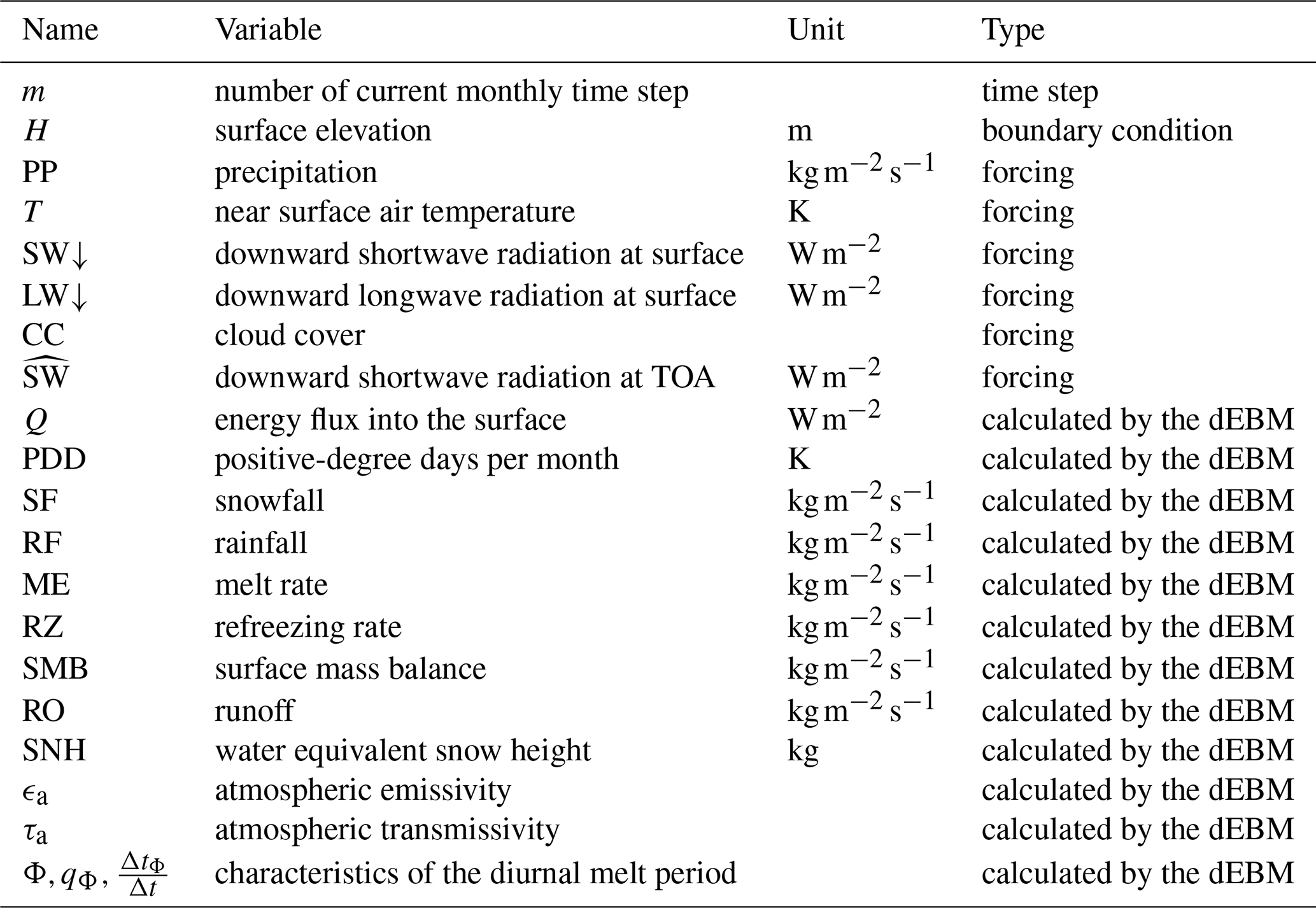
The surface mass balance scheme dEBM (diurnal Energy Balance Model) provides a novel interface between the atmosphere and land ice for Earth system modeling, which is based on the energy balance of glaciated surfaces. In contrast to empirical schemes, dEBM accounts for changes in the Earth’s orbit and atmospheric composition. The scheme only requires monthly atmospheric forcing (precipitation, temperature, shortwave and longwave radiation, and cloud cover). It is also computationally inexpensive, which makes it particularly suitable to investigate the ice sheets' response to long-term climate change. After calibration and validation, we analyze the surface mass balance of the Greenland Ice Sheet (GrIS) based on climate simulations representing two warm climate states: a simulation of the mid-Holocene (approximately 6000 years before present) and a climate projection based on an extreme emission scenario which extends to the year 2100. The former period features an intensified summer insolation while the 21st century is characterized by reduced outgoing longwave radiation. Specifically, we investigate whether the temperature–melt relationship, as used in empirical temperature-index methods, remains stable under changing insolation and atmospheric composition. Our results indicate that the temperature–melt relation is sensitive to changes in insolation on orbital timescales but remains mostly invariant under the projected warming climate of the 21st century.

1 Introduction

At the surface, land ice gains mass through snow accumulation and loses mass through meltwater runoff and sublimation. The total surface mass balance (SMB) of a healthy ice sheet (i.e., not in the process of disintegration) needs to be positive in the long term, in order to compensate for mass loss at the base, the peripheral surface and the interfaces to oceans or proglacial lakes. The SMB exerts an essential control on the volume and geometry of ice sheets. Responding directly to climate change, the SMB substantially influences the waxing and waning of large-scale ice sheets in the course of glacial–interglacial cycles on timescales of tens of thousands to 100 000 years (e.g., Hays et al., 1976; Huybers, 2006). The last glacial period was terminated by a rapid deglaciation, which caused the global sea level to rise by more than 100 m within 10 000 years (e.g., Lambeck et al., 2014) and resulted in a complete disintegration of the North American and Fennoscandian Ice Sheet (e.g., Peltier et al., 2015). In the present interglacial period, the Holocene, the Greenland Ice Sheet is the only ice sheet remaining on the Northern Hemisphere. Today, superimposed on the natural glacial–interglacial cycle, the anthropogenic climate change will likely initiate an unprecedented, anthropogenic deglaciation. The Greenland Ice Sheet is presently shrinking, and surface processes are predicted to amplify Greenland ice loss in the future (Oppenheimer et al., 2021).

Ice sheet models forced by different climate projections predict a reduction in the mass of the Greenland Ice Sheet by the end of this century, which could, according to high-emission scenarios, contribute 9±5 cm to sea level rise from 2015 to 2100 (Goelzer et al., 2020). This assessment is in general agreement with earlier studies based on fewer ice sheet models and different SMB forcing (Rueckamp et al., 2019; Fuerst et al., 2015). Aschwanden et al. (2019) demonstrate that gradually increasing surface runoff will become the predominant reason for GrIS mass loss under the projected warming of the coming centuries. In the 2002–2017 period, the Greenland Ice Sheet and surrounding glaciers contributed a total of 1 cm to sea level rise as measured by the Gravity Recovery and Climate Experiment (GRACE; Tapley et al., 2004). Reduced SMB explains more than half of the mass loss of the Greenland Ice Sheet (GrIS) (Sasgen et al., 2012). The change in SMB, primarily due to intensified meltwater runoff, has been attributed to positive air temperature anomalies, a more extended melt period (e.g., Tedesco and Fettweis, 2012) and a reduction in cloud cover (Hofer et al., 2017). The GRACE observational period is characterized by several summers of extreme melt in Greenland, and year-to-year changes in GrIS mass loss are large in comparison to the general acceleration over the full GRACE period. Specifically, the 2003–2013 period of accelerating mass loss and the subsequent deceleration are mostly associated with atmospheric circulation change (Greenland blocking, e.g., Fettweis et al., 2013; Bevis et al., 2019). To understand and predict the response of continental ice sheets to a changing climate, it is critical to reliably diagnose the SMB component. A reliable estimate of the SMB can be produced either (a) with empirical approaches or (b) from consideration of the surface energy balance in physics-based schemes. Empirically, the SMB of the GrIS can be estimated from near-surface air temperatures, for instance, by the positive-degree-day method (Reeh, 1991). This particularly simple approach linearly relates mean melt rates to positive-degree days, PDDs; PDD refers to the temporal integral of near-surface temperatures (T) exceeding the melting point, (e.g., Calov and Greve, 2005). Since this scheme has a low computational cost and is easy to handle, it has been widely used for long climate simulations (Charbit et al., 2013; Gierz et al., 2015; Heinemann et al., 2014; Roche et al., 2014; Ziemen et al., 2014) and paleo-temperature reconstructions (Box, 2013; Wilton et al., 2017). The PDD method was calibrated based on SMB observations from the GrIS and has demonstrated a good skill to reproduce recent changes in Greenland surface mass balance (Fettweis et al., 2020). However, changes in insolation due to long-term changes in the Earth's orbit can influence the sensitivity of the SMB to temperature (van de Berg et al., 2011; Robinson and Goelzer, 2014). Also, field measurements from glaciers outside of Greenland reveal that optimal parameters for the PDD scheme strongly differ for different latitudes, altitudes or climate zones (Hock, 2003). Therefore it is questionable whether the empirical Greenland-based parameterization can be applied to ice sheets outside of Greenland (e.g., the ice sheets of the last ice age) or in different climates.

In contrast to empirical approaches, physics-based (and thus more universal) surface mass balance schemes for ice sheets and glaciers consider the sum of all energy fluxes Q into the surface layer to calculate surface melt and refreezing of meltwater. If the surface temperature is at the melting point, the melt rate is linearly related to the surface layer's net energy uptake. Refreezing is analogously related to a net heat release, but refreezing is limited by the amount of available liquid water. This asymmetry between melting and refreezing implies that unresolved (spatial or temporal) variations in Q around melting point result in underestimation of meltwater runoff. Consequently, SMB calculations based on the energy balance should resolve the region where Q>0 in summer and should also resolve the diurnal melt–freeze cycle, which is particularly pronounced for clear-sky conditions. Away from their mostly steep margins, ice sheets usually rise to high elevations and are exposed to cold air temperatures. Therefore, melting occurs in a narrow strip along the ice sheets' margins, which requires a resolution that is still beyond the scope of multidecadal global climate simulations or reanalysis products such as ERA-Interim (Dee et al., 2011). SMB estimates thus commonly involve some downscaling of coarse-resolution forcing, either (i) dynamically through high-resolution regional climate models, such as MAR (Fettweis et al., 2017), RACMO, (Noël et al., 2018), HIRHAM, (Langen et al., 2015) or NHM-SMAP (Niwano et al., 2018); (ii) through the implementation of a one-dimensional SMB module in the climate model which recalculates the energy balance on different elevation classes (Vizcaino et al., 2010); or (iii) through downscaling of coarse-resolution climate forcing according to the high-resolution topography for stand-alone SMB modeling (e.g., Born et al., 2019; Krapp et al., 2017). Overall, regional climate models perform best in comparison to observations as was demonstrated in the Greenland Surface Mass Balance Intercomparison Project (GrSMBMIP; Fettweis et al., 2020), which is primarily related to a better representation of topographic precipitation. The computational cost of regional climate models prohibits the use of these models on millennial timescales, which is necessary to study the slow response of ice sheets in a changing climate. Downscaling SMB via elevation classes within Earth system models is a relatively complex yet less costly approach, and first applications yield promising results (e.g., Vizcaino et al., 2010; van Kampenhout et al., 2019). Its tight integration into an Earth system model prohibits its use as a flexible stand-alone SMB model. Stand-alone SMB models for long-term Earth system modeling usually realize spatial downscaling by a lapse rate correction of coarse-resolution temperatures to high-resolution topography. These efficient SMB schemes either involve empirical parameterizations which are not necessarily climate independent (Plach et al., 2018; de Boer et al., 2013) or usually require at least daily forcing. The BErgen Snow SImulator (BESSI; Born et al., 2019) uses a daily time step and considers the surface energy balance in combination with a sophisticated multi-layer snowpack model. BESSI appears to underestimate refreezing possibly because diurnal freeze–melt cycles are not resolved. The Surface Energy and Mass balance model of Intermediate Complexity (SEMIC; Krapp et al., 2017) also uses a daily time step but statistically accounts for diurnal variations in surface temperature. Following a similar approach Krebs-Kanzow et al. (2018b) demonstrated that the diurnal melt period can be downscaled from monthly mean forcing by using the knowledge of the diurnal cycle of insolation at the top of the atmosphere, which is a function of latitude and season.

Here we refine the approach of Krebs-Kanzow et al. (2018b) and present a novel stand-alone SMB model, dEBM. The presented model is efficient on millennial timescales and particularly suitable for Earth system modeling on long timescales in a modular framework such as Gierz et al. (2020), as it only requires monthly forcing. The scheme now also includes an albedo scheme, accounts for changes in atmospheric composition and statistically resolves submonthly variability in cloud cover. In the following section of this paper, we provide a detailed model description. We then discuss the calibration of model parameters and evaluate the model against observations and a regional climate model. Finally, we apply dEBM with climate forcing from a simulation of the mid-Holocene warm period and from a transient climate simulation from the preindustrial period to the year 2100 based on the RCP8.5 scenario (Taylor et al., 2012). We specifically analyze the sensitivity of meltwater runoff to temperature change for these two distinct warm periods, to assess the validity of the empirical PDD method for different background climates. In the Appendix, Tables A1 and A2 provide a list of parameters and variables.

2 Model description

2.1 General concept

The dEBM is based on the surface energy balance and simulates surface mass balance (SMB), melting (ME), refreezing (RZ), snowfall (SF), snow height (SNH), net runoff (RO) and albedo (A) at monthly time steps. The model is formulated with a focus on the ablation zone; if surface conditions do not favor surface melt, the surface mass balance is exclusively controlled by the accumulation of snow. As forcing, the model requires monthly means of total precipitation (PP_cr), near-surface air temperature (T_cr), incoming surface shortwave radiation (SW${}_{\mathrm{cr}}^{\downarrow }$), top-of-atmosphere (TOA) incoming shortwave radiation $\widehat{\mathrm{SW}}$, incoming longwave radiation (LW${}_{\mathrm{cr}}^{\downarrow }$) and cloud cover (CC_cr), and as a boundary condition it requires the surface elevation H_cr consistent with the forcing data. The suffix _cr is given to the quantities, as usually, a coarse-resolution climate model provides these forcing fields. Furthermore a target grid of sufficient resolution needs to be defined, and respective high-resolution surface elevation data H need to be available.

Preparatory processing and downscaling of the forcing (Sect. 2.4). In the following, H_int, T, PP, SW^↓, LW^↓ and CC denote the respective monthly mean variables after downscaling or interpolating to the target grid. The spatial downscaling scheme involves a simple elevation correction of T_cr by applying a spatially and temporally constant lapse rate. The concept of the temporal downscaling is to separately diagnose radiation for “fair” and “cloudy” days and to proportionally account for these days according to monthly mean cloud cover. This temporal downscaling strategy is based on additional assumptions and is inspired by an analysis of PROMICE automatic weather station data (Ahlstrom et al., 2008). These observations from the GrIS reveal that daily cloudiness is not normally distributed but forms two clusters (Fig. 1) with distinct radiative characteristics (Fig. 2).

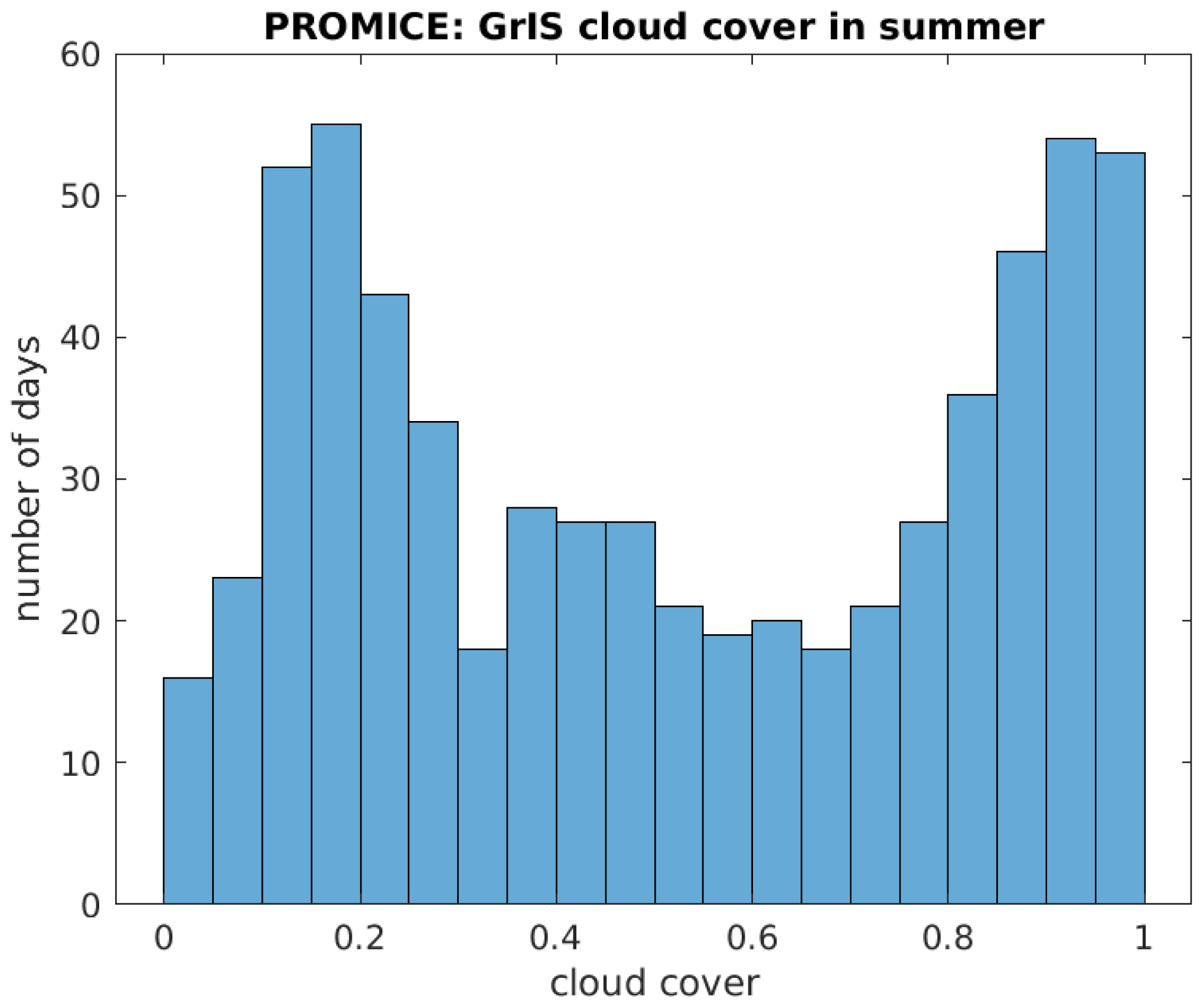
Figure 1 Histogram of daily cloud cover over the Greenland Ice Sheet throughout the summer months (June, July, August) based on daily measurements from up to 11 years of daily observations from 17 PROMICE weather stations.

Melting and refreezing periods (Sect. 2.3). We separately diagnose monthly melt and refreezing rates from submonthly periods of positive and negative surface energy balance, respectively (Sect. 2.3). We consider the surface energy balance of three different cases: the energy balance of cloudy days, Q_cloudy, and of fair days, Q_fair, and for fair days, we additionally consider the surface energy balance of the diurnal melt period Q_MP. Here and in the following, _MP denotes quantities relevant during the melt period of fair days. The energy balance of the downscaled submonthly periods Q_cloudy,Q_MP and Q_fair−Q_MP then yields respective melt or refreezing rates which contribute to the monthly surface mass balance (Sect. 2.2). The albedo scheme (Sect. 2.6) accounts for an important positive feedback: melting lowers the albedo of a snow surface, which in turn increases the energy uptake from shortwave radiation and re-intensifies melting. In consequence the ablation zone is distinguished by the lower albedo of wet snow and bare ice from the accumulation zone with higher albedos of dry and fresh snow. The dEBM distinguishes three surface types with distinct albedos: bright new snow, dry snow and dark wet show. The surface type of each grid point is assigned after an evaluation of the potential surface mass balance for each surface type, which implies that the surface energy balance is preliminarily calculated three times using the respective albedo values.

2.2 The surface mass balance

The main components determining the surface mass balance and the ice sheet's meltwater runoff (RO)

$$\begin{array}{}\text{(1)}& \begin{array}{rl}\mathrm{SMB}& =\mathrm{SF}-\mathrm{ME}+\mathrm{RZ}\\ \mathrm{RO}& =\mathrm{ME}+\mathrm{RF}-\mathrm{RZ}\end{array}\end{array}$$

are discussed individually in the following.

Snowfall SF.

SF(PP, T) is a function of precipitation and near-surface air temperature as described in Sect. 2.4.

Rainfall RF.

RF(PP, T) = PP − SF is a function of precipitation and near-surface air temperature as described in Sect. 2.4.

Surface melt rate ME.

Melting is assumed to be only possible if monthly mean near-surface temperature exceeds a minimum temperature, T_min. As in Krebs-Kanzow et al. (2018b), we choose T_min = −6.5 ^∘C. Under melting conditions, melt rates of cloudy days are linearly related to any positive net surface energy flux $max(\mathrm{0},Q_{\mathrm{cloudy}})$, and the melt rate of fair days is related to $max(\mathrm{0},Q_{\mathrm{fair}}$, Q_MP), with Q_cloudy,Q_fair being the surface energy balance of cloudy and fair days and Q_MP being the energy balance during the subdaily melt period of fair days (Sect. 2.3). In most cases Q_fair<Q_MP, as outgoing longwave radiation usually dominates the energy balance of a cold surface in clear nights (Sect. 2.3). The total melt rate is

$$\begin{array}{}\text{(2)}& \begin{array}{rl}\mathrm{ME}=& {\displaystyle \frac{\mathrm{1}}{\mathit{\rho }{L}_{\mathrm{f}}}}\left(\right(\mathrm{1}-\mathrm{CC}\left)\right(max(\mathrm{0},Q_{\mathrm{fair}},Q_{\mathrm{MP}}))\\ & +\mathrm{CC}max(\mathrm{0},Q_{\mathrm{cloudy}}))\end{array}\end{array}$$

with latent heat of fusion L_f and the density of liquid water ρ.

Refreezing rate RZ.

Analogous to melting, we assume that RZ is linearly related to negative net surface energy fluxes. The maximum potential refreezing rate is

$$\begin{array}{}\text{(3)}& \begin{array}{rl}{\mathrm{RZ}}_{\mathrm{pot}}=& {\displaystyle \frac{\mathrm{1}}{\mathit{\rho }{L}_{\mathrm{f}}}}(\mathrm{1}-\mathrm{CC})(min(\mathrm{0},Q_{\mathrm{fair}},Q_{\mathrm{fair}}-Q_{\mathrm{MP}}\left)\right)\\ & +\mathrm{CC}min(\mathrm{0},Q_{\mathrm{cloudy}}).\end{array}\end{array}$$

The total refreezing rate is limited by the amount of liquid water (from rainfall RF; see Sect. 2.4 or melting ME) and the storage capacity. Following the parameterization of Reeh (1991), we assume that the surface snow layer can hold 60 % of its mass, and the refreezing rate for the month m is

$$\begin{array}{}\text{(4)}& \begin{array}{rl}\mathrm{RZ}=& min\left(\left[(\mathrm{RF}+\mathrm{ME}),\right.\right.\\ & \left.\left.{\displaystyle \frac{\mathrm{0.6}\mathrm{SNH}(m-\mathrm{1}){\mathit{\rho }}_{\mathrm{water}}}{\mathrm{\Delta }{t}_m}},{\mathrm{RZ}}_{\mathrm{pot}}\right]\right).\end{array}\end{array}$$

SNH is the water equivalent snow height, which is a prognostic quantity; see Sect. 2.7 for details. m is the monthly time step, and Δt_m is the duration of month m, which is always a month here. Meltwater which does not refreeze within a month is added to the monthly runoff.

Other contributions to the SMB such as sublimation, evaporation and hoar are so far neglected by the dEBM as it is not expected that our downscaling approach can improve the respective mass fluxes if these are provided by climate models. In the framework of global climate models, these processes can be diagnosed on larger spatial scales but shorter time steps. With minor technical modifications, these fluxes can be individually added to snowfall (SF) and rainfall (RF) as an additional forcing (negative snowfall does not pose a problem).

2.3 The surface energy balance

We consider the surface energy balance of a melting surface. The energy balance of a melting surface can be simplified by applying the Stefan–Boltzmann law for longwave radiation with the snow and ice surface temperature at the melting point T_i=T₀. As surface temperature is not simulated by the dEBM, we define a simple temperature criterion for the near-surface air temperature T>T_min to identify potential melting conditions. We either rule out melting from the outset or estimate melt rates from this simplified energy balance, depending on near-surface air temperature (T), incoming shortwave radiation (SW^↓) and albedo (A(SurfaceType)), which is chosen according to the given surface types (i.e., NewSnow, DrySnow or WetSnow), and further differentiate these for cloudy and fair conditions following Willeit and Ganopolski (2018):

$$\begin{array}{}\text{(5)}& \begin{array}{rl}Q=& (\mathrm{1}-A){\mathrm{SW}}^{\downarrow }+a(T-T_{\mathrm{0}})+b\\ a=& {\mathit{ϵ}}_{\mathrm{i}}{\mathit{ϵ}}_{\mathrm{a}}\mathit{\sigma }\mathrm{4}{T}_{\mathrm{0}}^{\mathrm{3}}+\mathit{\beta }\\ b=& -{\mathit{ϵ}}_{\mathrm{i}}\mathit{\sigma }{T}_{\mathrm{0}}^{\mathrm{4}}+{\mathit{ϵ}}_{\mathrm{a}}{\mathit{ϵ}}_{\mathrm{i}}\mathit{\sigma }\left(T_{\mathrm{0}}^{\mathrm{4}}\right)+R,\end{array}\end{array}$$

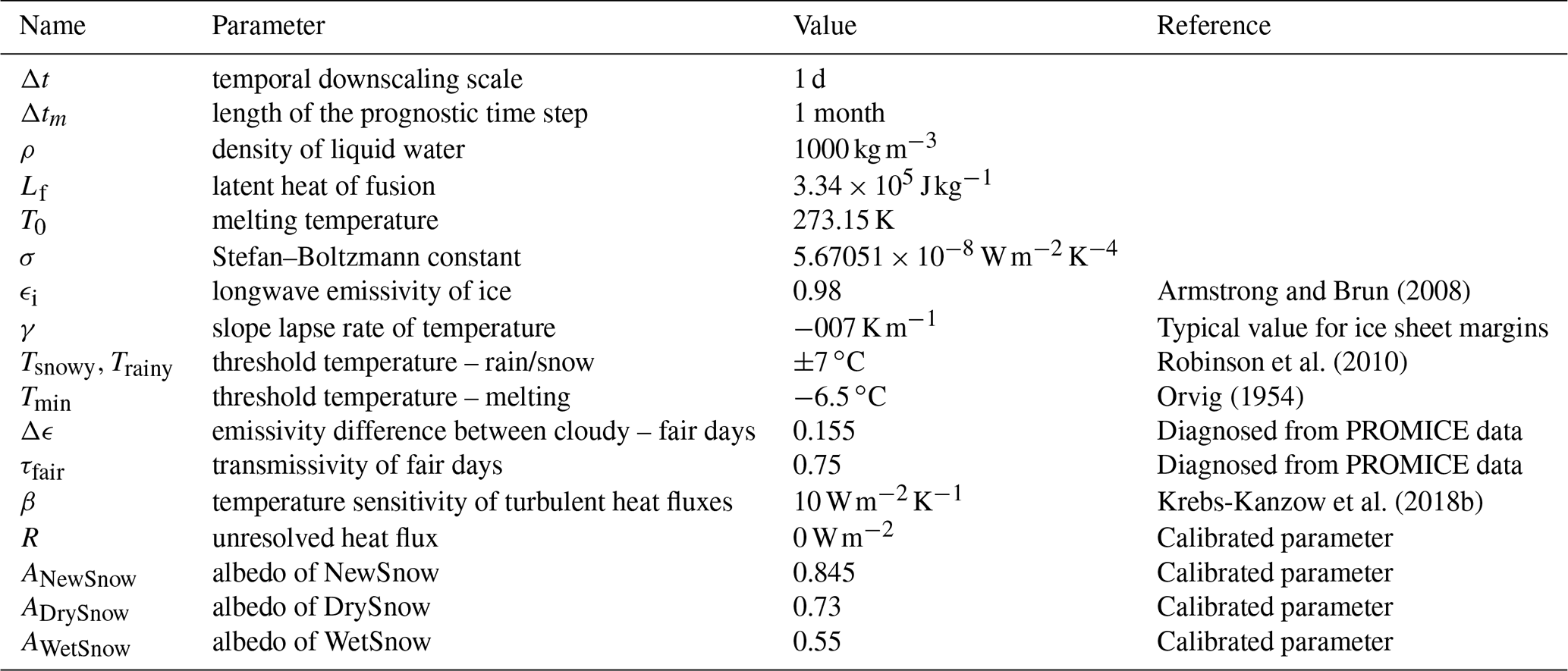
where ϵ_i and ϵ_a are the longwave emissivities of ice and atmosphere, σ is the Stefan–Boltzmann constant, the coefficient β represents the temperature sensitivity of the turbulent heat flux and T₀ is the melting point. We use a constant ϵ_i=0.98 (Armstrong and Brun, 2008) and locally diagnose ϵ_a from the longwave radiation and air temperature forcing. We define that all fluxes into the ice sheet's surface layer are positive. The term R represents all unresolved energy fluxes, such as temperature-independent turbulent heat fluxes and heat conduction to the subsurface.

In contrast to Krebs-Kanzow et al. (2018b), parameters a and b are not constant because the atmospheric emissivity is diagnosed from longwave radiation and near-surface temperature. Since Q_fair and Q_cloudy are separately calculated (Eq. 5), the monthly shortwave radiation SW${}_{\mathrm{cloudy}/\mathrm{fair}}^{\downarrow }$, albedo $A_{\mathrm{cloudy}/\mathrm{fair}}$ and atmospheric emissivity ${\mathit{ϵ}}_{\mathrm{a},\mathrm{cloudy}/\mathrm{fair}}$ are also differentiated between cloudy and fair conditions (Sect. 2.4).

Following Krebs-Kanzow et al. (2018b), we also consider the energy balance of the daily melt period of fair days, which is defined to be that part of a day when the elevation angle of the sun exceeds a critical value so that incoming shortwave radiation exceeds outgoing longwave radiation. In contrast to Krebs-Kanzow et al. (2018b), we estimate the critical elevation angle Φ for each location to account for the spatial variability in atmospheric emissivity ϵ_a,fair. The energy balance of the daily melt period Q_MP is then

$$\begin{array}{}\text{(6)}& Q_{\mathrm{MP}}=\left((\mathrm{1}-A){\mathrm{SW}}_{\mathrm{MP}}^{\downarrow }+a_{\mathrm{MP}}{T}_{\mathrm{MP}}+b_{\mathrm{MP}}\right),\end{array}$$

where Q_MP represents a monthly mean energy flux with

$$\begin{array}{}\text{(7)}& \begin{array}{rl}{\mathrm{SW}}_{\mathrm{MP}}& ={\displaystyle \frac{\mathrm{\Delta }{t}_{\mathrm{\Phi }}}{\mathrm{\Delta }t}}{q}_{\mathrm{\Phi }}{\mathrm{SW}}_{\mathrm{fair}}\\ a_{\mathrm{MP}}& ={\displaystyle \frac{\mathrm{\Delta }{t}_{\mathrm{\Phi }}}{\mathrm{\Delta }t}}{\mathit{ϵ}}_{\mathrm{i}}{\mathit{ϵ}}_{\mathrm{a},\mathrm{fair}}\mathit{\sigma }\mathrm{4}{T}_{\mathrm{0}}^{\mathrm{3}}+\mathit{\beta }\\ b_{\mathrm{MP}}& ={\displaystyle \frac{\mathrm{\Delta }{t}_{\mathrm{\Phi }}}{\mathrm{\Delta }t}}\left(-{\mathit{ϵ}}_{\mathrm{i}}\mathit{\sigma }{T}_{\mathrm{0}}^{\mathrm{4}}+{\mathit{ϵ}}_{\mathrm{a},\mathrm{fair}}{\mathit{ϵ}}_{\mathrm{i}}\mathit{\sigma }\left(T_{\mathrm{0}}^{\mathrm{4}}\right)+R\right).\end{array}\end{array}$$

T_MP is the near-surface temperature T_MP during the melt period. T_MP is parameterized by the positive-degree days per month as defined in Sect. 2.4. The Δt_Φ is the length of the melt period when the sun exceeds the elevation angle Φ. The ratio $\frac{\mathrm{\Delta }{t}_{\mathrm{\Phi }}}{\mathrm{\Delta }t}$ converts the energy flux during the melt period to daily fluxes. The q_Φ is the ratio $\frac{{\mathrm{SW}}_{\mathrm{\Phi }}}{{\mathrm{SW}}_{\mathrm{0}}}$ (surface shortwave radiation averaged over the daily melt period relative to shortwave radiation averaged over the whole day). The parameters q_Φ and Δt_Φ are functions of the elevation angle Φ, which is calculated locally here as we use spatially variable atmospheric emissivity.

2.4 Preprocessing of the climate forcing

The following downscaling steps are conducted prior to the actual SMB simulation to represent submonthly variability and spatially unresolved topographic features.

2.4.1 Monthly mean atmospheric emissivity

According to the Stefan–Boltzmann law, downward longwave radiation can be expressed as a function of atmospheric emissivity and temperature:

$$\begin{array}{}\text{(8)}& \mathrm{LW}({\mathit{ϵ}}_{\mathrm{a}},T)={\mathit{ϵ}}_{\mathrm{a}}\mathit{\sigma }{T}^{\mathrm{4}}.\end{array}$$

In preparation of the downscaling of longwave radiation, we use Eq. (8) to diagnose ϵ_a,cr from coarse-resolution downward longwave radiation and near-surface temperatures.

2.4.2 Interpolation

A bilinear interpolation between the source grid and the higher resolved target grid generates the fields of H_int, T_int SW^↓, ϵ_a, PP, CC and $\widehat{\mathrm{SW}}$.

2.4.3 Spatial downscaling: lapse rate correction of air temperature

We use a lapse rate of $\mathit{\gamma }=-\mathrm{0.007}$ K m⁻¹ to transform the near-surface temperature to the surface elevation H_ice of the target grid according to

$$\begin{array}{}\text{(9)}& T=T_{\mathrm{int}}+\mathit{\gamma }(H_{\mathrm{ice}}-H_{\mathrm{int}}).\end{array}$$

H_ice may originate from an ice sheet simulation or reconstruction and thus may differ substantially from the topography used in the climate model (H_int). The lapse-rate-corrected temperatures in combination with the interpolated ϵ_a can be used to spatially downscale longwave radiation by applying the Stefan–Boltzmann law. This spatial downscaling of longwave radiation is here combined with a statistical downscaling of submonthly variability, as detailed below.

2.4.4 Rain and snow

Precipitation is partitioned into snowfall (SF) and rainfall (RF) according to the downscaled temperatures T following Robinson et al. (2010), where SF=f(T)PP_int, with the solid fraction of the monthly mean precipitation, f(T), following a sine function from 1 to 0 between threshold temperatures $T_{\mathrm{snowy}}=-\mathrm{7}$ ^∘C and T_rainy=7 ^∘C. Below and above these thresholds all precipitation is considered to be snow and rain, respectively.

2.4.5 Statistical downscaling of radiative fluxes for fair and cloudy conditions

We fractionate downward longwave radiation and shortwave radiation for fair and cloudy conditions:

$$\begin{array}{}\text{(10)}& \begin{array}{rl}\mathrm{SW}\downarrow & =\mathrm{CC}{\mathrm{SW}}_{\mathrm{cloudy}}^{\downarrow }+(\mathrm{1}-\mathrm{CC}){\mathrm{SW}}_{\mathrm{fair}}^{\downarrow }\\ \mathrm{LW}\downarrow & =\mathrm{CC}{\mathrm{LW}}_{\mathrm{cloudy}}^{\downarrow }+(\mathrm{1}-\mathrm{CC}){\mathrm{LW}}_{\mathrm{fair}}^{\downarrow }.\end{array}\end{array}$$

To avoid numeric problems, we only apply this separation if monthly cloud cover is in the range of [0.1 0.9] and otherwise use unseparated SW↓ and LW↓ to calculate the energy balance Q, accounting (not accounting) for the diurnal melt period during the entire month, if CC<0.1 (CC>0.9).

Where we separate cloudy and fair conditions, we need to introduce two additional assumptions which are based on an analysis of PROMICE automatic weather station data here (Ahlstrom et al., 2008). Specifically we analyze daily radiation, cloud cover and air temperature observations from 17 stations, which cover up to 11 years (Fig. 2). Applying Eq. (8), we diagnose distinct atmospheric emissivities ϵ_fair and ϵ_cloudy for fair or cloudy conditions, and similarly we diagnose atmospheric transmissivities τ_fair and τ_cloudy according to

$$\begin{array}{}\text{(11)}& {\mathrm{SW}}_{\mathrm{fair},\mathrm{cloudy}}^{\downarrow }={\mathit{\tau }}_{\mathrm{fair},\mathrm{cloudy}}\widehat{\mathrm{SW}}\end{array}$$

with atmospheric transmissivities τ_cloudy and τ_fair for fair and cloudy conditions.

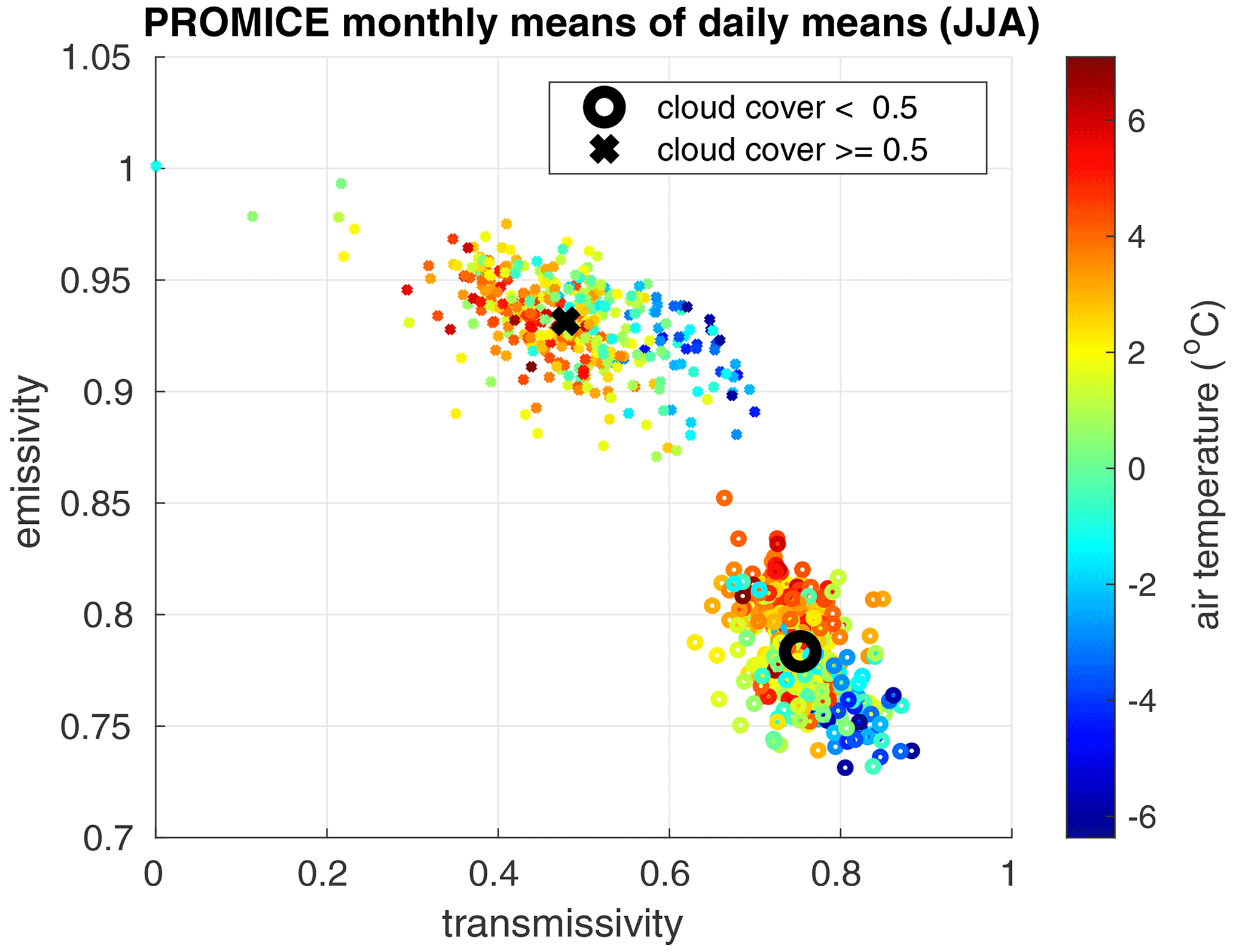
Figure 2 Monthly mean emissivities versus transmissivities for fair and cloudy conditions, ${\stackrel{\mathrm{‾}}{\mathit{ϵ}}}_{\mathrm{fair}}$, ${\stackrel{\mathrm{‾}}{\mathit{ϵ}}}_{\mathrm{cloudy}}$, ${\stackrel{\mathrm{‾}}{\mathit{\tau }}}_{\mathrm{fair}}$ and ${\stackrel{\mathrm{‾}}{\mathit{\tau }}}_{\mathrm{cloudy}}$ of all summer months as calculated from up to 11 years of daily observations from 17 PROMICE weather stations. Every symbol represents the respective parameters as diagnosed for one individual month at one station. Colors reflect the respective air temperature measurements. Black symbols represent the respective dataset means.

To do so we classify all summer days (June to August) with cloud cover ≥ 50 % as “cloudy” and otherwise as “fair” and calculate monthly mean ϵ_fair, ϵ_cloudy, τ_fair and τ_cloudy.

Under fair conditions atmospheric transmissivity τ_fair is relatively well constrained (Fig. 2). Therefore, we use τ_fair=0.75 to diagnose SW${\downarrow }_{\mathrm{fair}}={\mathit{\tau }}_{\mathrm{fair}}\widehat{\mathrm{SW}}$ and SW${\downarrow }_{\mathrm{cloudy}}=\frac{\mathrm{1}}{\mathrm{CC}}(\mathrm{SW}\downarrow -(\mathrm{1}-\mathrm{CC}\left)\mathrm{SW}{\downarrow }_{\mathrm{fair}}\right)$ from Eq. (11).

To separate longwave radiation, we constrain atmospheric emissivities by defining Δϵ to be the emissivity increase due to cloud cover with

$$\begin{array}{}\text{(12)}& {\mathit{ϵ}}_{\mathrm{cloudy}}={\mathit{ϵ}}_{\mathrm{fair}}+\mathrm{\Delta }\mathit{ϵ}.\end{array}$$

This is in line with parameterizations which assume that greenhouse gas concentration (which is primarily water vapor) and cloud cover will influence the atmospheric emissivity independently (e.g., König-Langlo and Augstein, 1994). The difference between ϵ_fair and ϵ_cloudy is thus assumed to be constant, and both values are equally affected by greenhouse gases. For a given Δϵ, we can determine

$$\begin{array}{}\text{(13)}& \begin{array}{rl}{\mathit{ϵ}}_{\mathrm{fair}}& ={\mathit{ϵ}}_{\mathrm{a}}-\mathrm{CC}\mathrm{\Delta }\mathit{ϵ}\\ {\mathit{ϵ}}_{\mathrm{cloudy}}& ={\mathit{ϵ}}_{\mathrm{a}}+(\mathrm{1}-\mathrm{CC})\mathrm{\Delta }\mathit{ϵ}.\end{array}\end{array}$$

According to König-Langlo and Augstein (1994) and Sedlar and Hock (2009) the emissivity difference will be Δϵ≈0.21 if cloudy and fair conditions correspond to a cloud cover of 100 % and 0 %, respectively. This value is not realistic, because partially cloud-covered days occur frequently (Fig. 1), and emissivity and cloud cover are not linearly related. Instead Fig. 2 indicates that Δϵ≈0.155, which is the value we use to separate longwave radiation in all following applications.

In Fig. 2 parameters reveal a temperature dependence which is predominantly associated with the elevation range of the PROMICE stations. The cloud thickness may be reduced at high elevations, and τ_cloudy is therefore elevation dependent. For τ_fair (the empirical parameter in our downscaling) the elevation effect is small by comparison. The temperature dependence in emissivities ϵ_fair,cloudy is in part related to the larger water vapor content of warmer air and is implicitly accounted for, as we do not constrain ϵ_fair but only prescribe Δϵ.

Positive-degree days

To parameterize the mean temperature of the diurnal melt period T_MP from monthly mean temperatures, we resort to positive-degree days per month, PDD, here defined to be the temporal integral of near-surface temperatures T exceeding the melting point per month. As in Krebs-Kanzow et al. (2018b) we use T_MP=PDD_3.5, with PDD_3.5 approximated as in Calov and Greve (2005) from monthly mean near-surface temperature ${\stackrel{\mathrm{‾}}{T}}_{\mathrm{a}}$ and a constant standard deviation of std_T=3.5 ^∘C.

2.5 Initialization and forward integration

For a transient simulation, we initialize the model with no initial snow cover (SNH =0) and, for Northern Hemisphere applications, start the integration with October, the beginning of the hydrological year. After December, we continue the integration (re)using the forcing of the first year for two 12-month cycles. The first 15 months are considered to be a spin-up, the following second full cycle is the first year of the actual simulation. At the end of each month, snow height is updated according to its surface mass balance (Sect. 2.7). After September we additionally subtract the snow height of the previous year's September, which corresponds to the assumption that snow which is by then older than a year will transform into ice. On the Southern Hemisphere, the integration should start in April, and snow should transform to ice by the end of March.

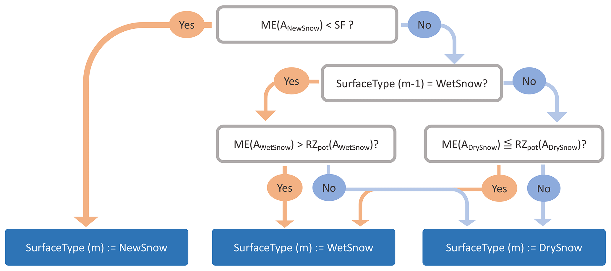
Figure 3 Schematic of the algorithm which selects the surface type (NewSnow, DrySnow or WetSnow) for each grid point and month m.

2.6 The albedo scheme

Surface melt decreases the albedo of snow and ice, and at the same time a lowered albedo intensifies surface melt. This strong positive feedback is a particularly crucial mechanism accelerating the recent mass loss of the GrIS (Box et al., 2012). The albedo of ice and snow is thus a critical parameter in any surface mass balance estimate which is based upon the balance of radiative and turbulent energy fluxes. The dEBM distinguishes three surface types: new snow, A_NewSnow; dry snow, A_DrySnow; and wet snow or ice, A_WetSnow. Each surface type is assigned a pair of albedo values for fair and cloudy conditions. Following Willeit and Ganopolski (2018), we assume that the albedo for cloudy conditions exceeds the respective albedo for fair conditions of the same surface type by 0.05. To determine the local surface type for a given month, we preliminarily calculate for these ME(A_SurfaceType) and RZ_pot(A_SurfaceType) as a function of albedo for each surface type. The local albedo is then determined by testing a sequence of logical conditions which are illustrated as a decision tree in Fig. 3. The scheme first tests whether the new snow of that month is likely to survive. If this is not the case the scheme includes some element of persistence: if snow was wet (dry) in the previous month it is first tested whether conditions allow that the surface remains wet (dry).

2.7 Snow height

At the end of every month m we update the height of the surface snow layer according to

$$\begin{array}{}\text{(14)}& \mathrm{SNH}\left(m\right)=max(\mathrm{0},\mathrm{SNH}(m-\mathrm{1}\left)\right)+{\displaystyle \frac{\mathrm{\Delta }{t}_m}{\mathit{\rho }}}(\mathrm{SF}-\mathrm{ME}+\mathrm{RZ}).\end{array}$$

where Δt_m is the length of month m. It is important to note that, between months, water cannot be stored within the snow column. That part of the monthly produced meltwater which does not refreeze within the same month will be removed from the snow column and will be added to the runoff. At the end of September we suppose that snow which is older than a year has been transformed to ice and accordingly reset snow height to

$$\begin{array}{}\text{(15)}& \mathrm{SNH}\left(m\right)=\mathrm{SNH}\left(m\right)-\mathrm{SNH}(m-\mathrm{12}).\end{array}$$

3 Parameter selection and evaluation based on observations

3.1 Experimental design

The albedo parameterization substantially influences the sensitivity of all SMB schemes which are based on the surface energy balance. The dEBM distinguishes three surface types, new snow, dry snow and wet snow, each associated with a distinct albedo. Similar surface types can be distinguished in observation. In field measurements on the western GrIS, Knap and Oerlemans (1996) observe albedos between 0.85 and 0.75 at higher altitudes and after the end of the melt season. Similarly Aoki et al. (2003) find that albedo of dry snow ranges between ≈ 0.85 for fresh snow and 0.75 for aged snow. During the melt season and near the ice edge, Knap and Oerlemans (1996) find a wide range of albedos for different surface types ranging from albedos around 0.45 for ice with ponds of surface water to mean albedos around 0.65 for superimposed ice (fragmented ice with an angular structure). On larger spatial scales and averaged over multiple days, however, areas of wet snow and ice typically exhibit albedos between 0.5 and 0.58 (Bøggild et al., 2010; Alexander et al., 2014; Riihelä et al., 2019). We conduct a series of calibration experiments with different parameter combinations for A_NewSnow, A_DrySnow and A_WetSnow together with the residual heat flux R (in Eq. 7). For fair conditions we vary A_NewSnow within $[\mathrm{0.84},\mathrm{0.845},\mathrm{0.85}]$, A_DrySnow within $[\mathrm{0.68},\mathrm{0.69},\mathrm{0.70},\mathrm{\dots },\mathrm{0.78}]$ and A_WetSnow within $[\mathrm{0.53},\mathrm{0.54},\mathrm{0.55},\mathrm{0.56},\mathrm{0.57}]$. The albedo values for cloudy conditions are varied with accordingly larger base values, and R varies within $[-\mathrm{2},-\mathrm{1},\mathrm{0},\mathrm{1},\mathrm{2}]$ W m⁻². These calibration experiments adapt the experimental design of Fettweis et al. (2020) and simulate the 1980–2016 SMB of the GrIS using monthly ERA-Interim forcing (Dee et al., 2011), which provides a resolution of 79 km and which is interpolated or downscaled by dEBM to the 1 km ISMIP6 grid (Nowicki et al., 2016). We evaluate these experiments based on two independent observational datasets. In the following we refer to these datasets as local observations and integral observations.

3.1.1 Local observations

We evaluate the calibration experiments based on local SMB measurements from Machguth et al. (2016) which are distributed around the ice sheet's margins and which provide integral SMBs over periods between months and multiple years. For each calibration experiment we bilinearly interpolate the simulated SMB of the four nearest grid cells of the ISMIP6 grid to the coordinates of the measurements and integrate simulated SMB over the respective observation period. Where observations do not cover full months the respective simulated monthly mean values contribute proportionally. We do not include observations which are outside of the ISMIP6 ice mask, which are not completely covered by the 1980–2016 period or which cover less than 3 months, which leaves 1252 local observations which primarily allow the assessment of the skill of the model to reproduce spatial characteristics of the SMB.

3.1.2 Integral observations

Also, we compare the simulated SMB to the 2003–2016 annual integral Greenland SMB derived from the sum of GRACE mass balance measurements $\frac{\mathrm{\Delta }M}{\mathrm{\Delta }t}$ (Sasgen et al., 2012, 2021) and interpolated monthly estimates of solid ice discharge D from Mankoff et al. (2019), assuming that SMB $=\frac{\mathrm{\Delta }M}{\mathrm{\Delta }t}+D$. Using the integral observations, we calculate annual SMB from October 2003 to September 2015 based on hydrologic years which start in October, which then provides the basis to assess the skill of the model to reproduce the integral SMB and its interannual variability.

3.2 Analysis of the calibration experiments

For the evaluation of the dEBM scheme, we take into account that the precipitation forcing is possibly biased: as precipitation is interpolated from the coarse-resolution ERA-Interim data, the intensified snow accumulation at the slopes and margins of the ice sheet may be systematically underestimated. Also low accumulation rates in the interior may be relatively inaccurate in the ERA-Interim reanalysis. Note that we do not optimize any parameters which affect snow accumulation, and errors in the forcing data may influence the calibration. Furthermore GRACE observations include regions of Greenland with seasonal snow cover and ice caps, which are not part of the ISMIP6 main ice sheet domain. We here assume that both errors in the interpolated ERA-Interim precipitation and the inconsistency of domains primarily affect the multi-year mean SMB of the GrIS but not so much its spatial or interannual variations. For this reason we separately evaluate the mean SMB and the variation around the mean with respect to the integral and local observations in order to choose a parameter combination which yields a good agreement with the variations around the mean for both datasets.

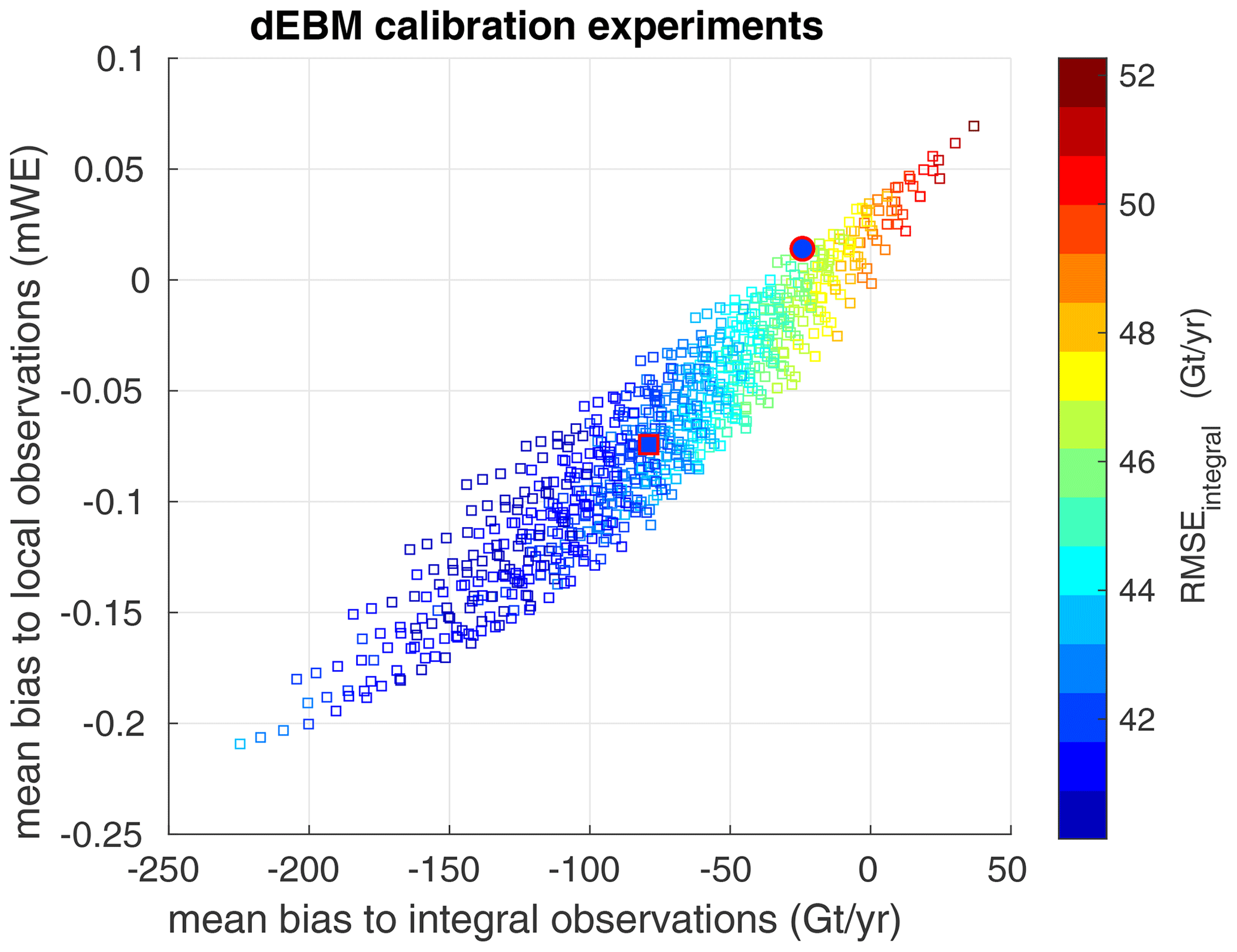
Figure 4 Mean bias of calibration experiments to integral observations as a function of the mean bias to local observations. The color represents the root-mean-square error of annual variations in the calibration experiments relative to the annual variations in the integral observations after the respective mean bias was removed. The experiment with the parameter combination which was selected for all following experiments is highlighted as a filled square with red borders. Also shown is experiment dEBM_MAR,ERA as a solid circle, which uses the same selected parameter combination but different forcing (see Sect. 4).

Figure 5 Root-mean-square error of the calibration experiments to temporal variations in the integral observation as a function of the root-mean-square error of calibration experiments to local observations. The mean bias between observations and calibration experiments has been removed before root-mean-square errors were calculated. Colors represent the mean bias of the calibration experiments to integral observations. The experiment with the parameter combination which was selected for all following experiments is highlighted as a filled square with red borders. Also shown is experiment dEBM_MAR,ERA as a solid circle, which uses the same selected parameter combination but different forcing (see Sect. 4).

We find that agreement of simulated mean SMB with observations is consistent between local and integral observations (Fig. 4) (low bias to local observations is also associated with low bias to integral observations), which indicates that the systematic bias over the entire period and domain is small in both datasets. Furthermore, we find multiple parameter combinations which yield reasonable agreement with both the temporal variations in the integral observations and the spatial structure in the local observations (Fig. 5). Good agreement with variations in both datasets (RMSE_integral<43 Gt and RMSE_local<0.557 mWE) is associated with a bias of approximately −80 Gt yr⁻¹ to the mean integral observations (Fig. 5) and a bias of approximately −0.07 mWE with respect to mean local observations. Closer inspection of the parameter combinations (not shown) which yield such good agreement reveals that combinations with $R=[\mathrm{0},\mathrm{1}]$ W m⁻², A_NewSnow=0.845, and A_WetSnow=0.55 or A_WetSnow=0.56 provide a generally good skill. Varying A_DrySnow in the range of [0.65 0.75] mostly influences whether agreement with local or integral observations is better.

Based on the calibration experiments, we choose the parameter combination of R=0 W m⁻², A_NewSnow=0.845, A_DrySnow=0.73 and A_WetSnow=0.55 for all following experiments. Using this combination together with the ERA-Interim forcing in experiment dEBM_ERA yields a good agreement with both the local and the integral observations.

4 Evaluation based on the regional climate model MAR

4.1 Experimental design

To compare dEBM to the regional model MAR, we conduct an experiment which follows the design of the calibration but uses a modified precipitation forcing. Experiment dEBM_MAR,ERA uses dynamically downscaled snow and rainfall from an ERA-Interim-forced simulation with the regional climate model MAR (experiment MAR_ERA; Fettweis et al., 2020). All other forcing fields are identical to the forcing used for the calibration experiments. The experiment MAR_ERA here also serves as a reference for comparison. The MAR simulation MAR_ERA was conducted in the framework of the Greenland Surface Mass Balance Intercomparison Project (GrSMBMIP) on an equidistant 15 km grid and was forced with 6-hourly ERA-Interim data at its lateral boundaries. This simulation was found to be in particularly good agreement with observations (Fettweis et al., 2020).

4.2 Evaluation of experiment dEBM_MAR,ERA

Replacing the precipitation forcing by MAR_ERA precipitation considerably improves the agreement with local observations. Furthermore, experiment dEBM_MAR,ERA exhibits a smaller mean bias to observations (Fig. 4 and Fig. 5), which supports our earlier hypothesis that the mean bias in experiment dEBM_ERA may be related to a systematically biased precipitation in the coarse-resolution ERA-Interim forcing. Experiments dEBM_MAR,ERA and MAR_ERA generally agree with respect to the evolution of integral, annual SMB (Fig. 6) with a root-mean-square error of 27 Gt. In comparison to the seasonal cycle of MAR, dEBM underestimates (overestimates) early (late) summer SMB, which indicates that dEBM fails to accurately reproduce onset and end of the annual melt season due to its monthly time step and missing processes such as snow aging, which may particularly bias late summer melt (Fig. 7). Integrated over the year these seasonal biasses mostly cancel out.

Figure 6 Annual mean integrated SMB in Gt yr⁻¹ of the Greenland Ice Sheet as derived from integral observations (black), and as simulated by MAR (blue) and dEBM (red).

Figure 7 The 1980–1999 multiyear monthly means of the GrIS SMB in Gt yr⁻¹ as simulated by MAR (blue) and dEBM (red) and their difference (dashed black).

We now evaluate the spatial representation of components of the SMB by comparing experiment dEBM_MAR,ERA to the MAR_ERA simulation for the period 1980 to 1999. By design the two simulations are identical in snow accumulation while variables which influence the meltwater runoff (i.e., temperatures, radiation and cloud cover) are dynamically consistent but not identical to the respective forcings used in dEBM_MAR,ERA. The presented MAR output has been interpolated or, in the case of air temperature and SMB, downscaled from its native 15 km resolution to the 1 km ISMIP6 grid. The temperature forcing of dEBM has been downscaled from ERA-Interim fields using a fixed lapse rate of 7 K km⁻¹ and generally exhibits a similar spatial structure. In comparison to MAR summer temperatures, we observe a large-scale warm bias over high-elevation North Greenland and mostly negative anomalies along the eastern margins of the ice sheets which can exceed 5 ^∘C around the complex East Greenland fjord systems around the Scoresby Sound. Large-scale patterns are inherent differences between ERA-Interim and MAR while local difference, especially at the coasts, may partly be a result of the relatively crude lapse rate correction of the dEBM forcing (Fig. 8).

Surface melt rates largely agree in the ablation zones of west and southeast Greenland (Fig. 9). Considerably weaker dEBM melt rates in the region of the Scoresby Sound can be attributed to the lower temperatures in the dEBM forcing, while lower melt rates at the southern tip of Greenland are not associated with respective differences in the temperature forcing. Stronger melting at the ice sheet's fringes is particularly visible in North Greenland and at the southeastern coast, which is also not always associated with warmer temperatures. Differences which are not explained by different temperature forcing may have a multitude of reasons: the simplicity of the dEBM albedo scheme, unresolved submonthly variability or the (neglected) effect of humidity and high wind speed on turbulent heat fluxes, which will be important at coastal locations. Finally dEBM seems to underestimate melting systematically at the upper boundary of the ablation zone. This is likely related to unrepresented submonthly temperature variability, as temperatures exhibit stronger variability at high elevations (Fausto et al., 2011) and the constant albedo for dry snow which cannot account for snow aging in low-accumulation regions of the interior GrIS. The weaker melting at higher elevations is in part compensated for by refreezing, which is generally weaker in dEBM than in MAR and especially in the higher parts of the ablation zone.

In total we find a good agreement between simulated SMB from dEBM and MAR, with differences being mostly restricted to narrow regions at the coast (Fig. 10).

The simulated albedo is closely linked to the simulated SMB. In the interior of the ice sheet, albedos simulated by dEBM are generally up to 0.05 higher than MAR albedos. Outside of the ablation zone MAR simulates a gradual transition towards higher albedos while dEBM always uses the new snow albedo of A_NewSnow=0.845 as soon as melt rates fail to exceed snowfall. If we use MAR as a reference, we find that within the ablation zone, dEBM seems to underestimate albedos in regions with high accumulation rates (southwest and southeast) while albedo is mostly overestimated in the north where accumulation rates are low and snow aging is important. Remarkably, higher (lower) albedo in the ablation zone is not necessarily associated with accordingly higher (lower) SMB or vice versa.

Figure 8 Comparison of multi-year (1980–1999) mean summer near-surface temperature from experiments MAR_ERA (a) and dEBM_MAR,ERA (b) and differences between dEBM_MAR,ERA and MAR_ERA (c).

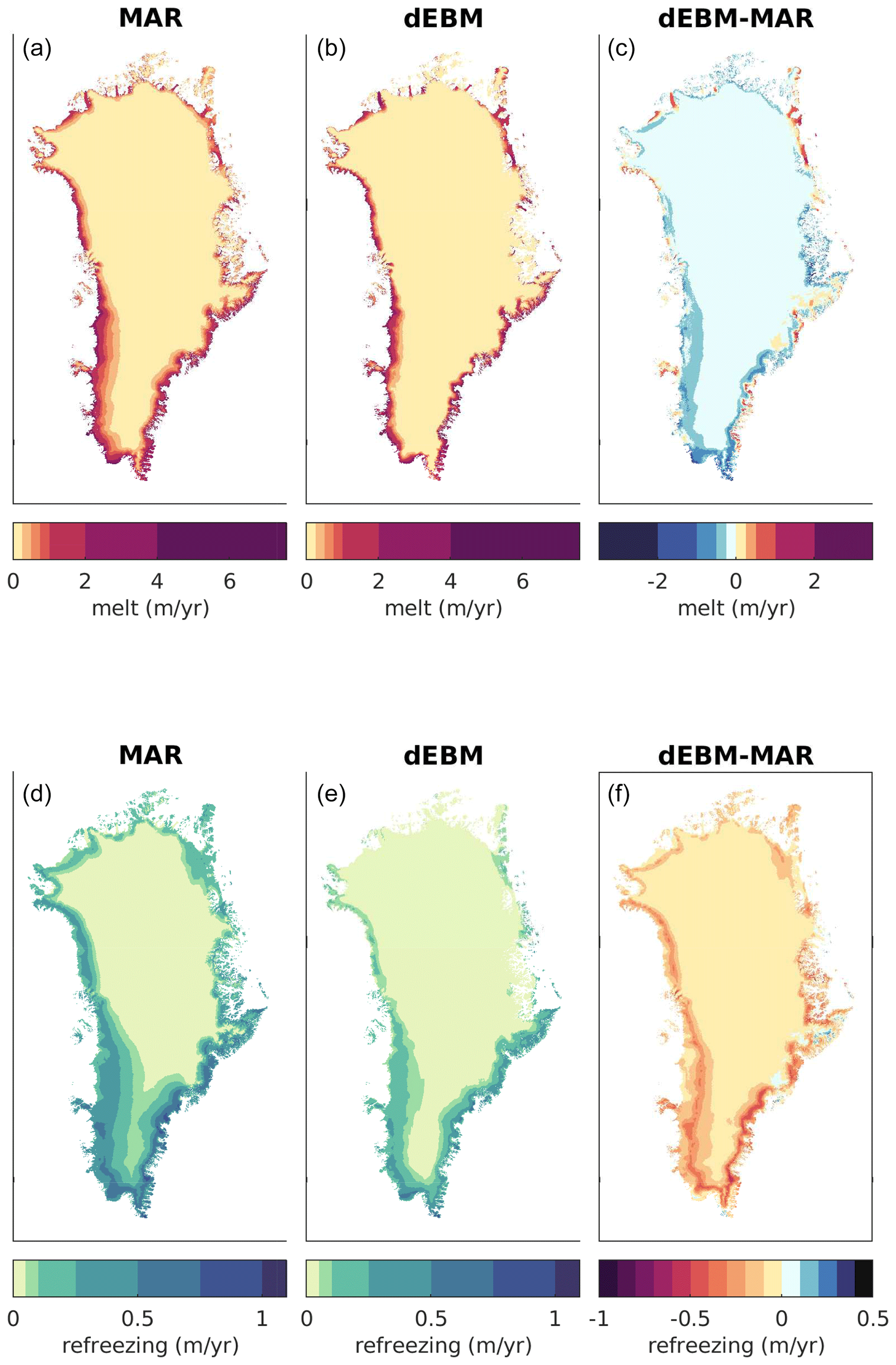
Figure 9 Comparison of multi-year (1980–1999) mean melt rates (a, b, c) and refreezing rates (d, e, f) from experiments MAR_ERA (a, d) and dEBM_MAR,ERA (b, e) and differences between dEBM_MAR,ERA and MAR_ERA (c, f).

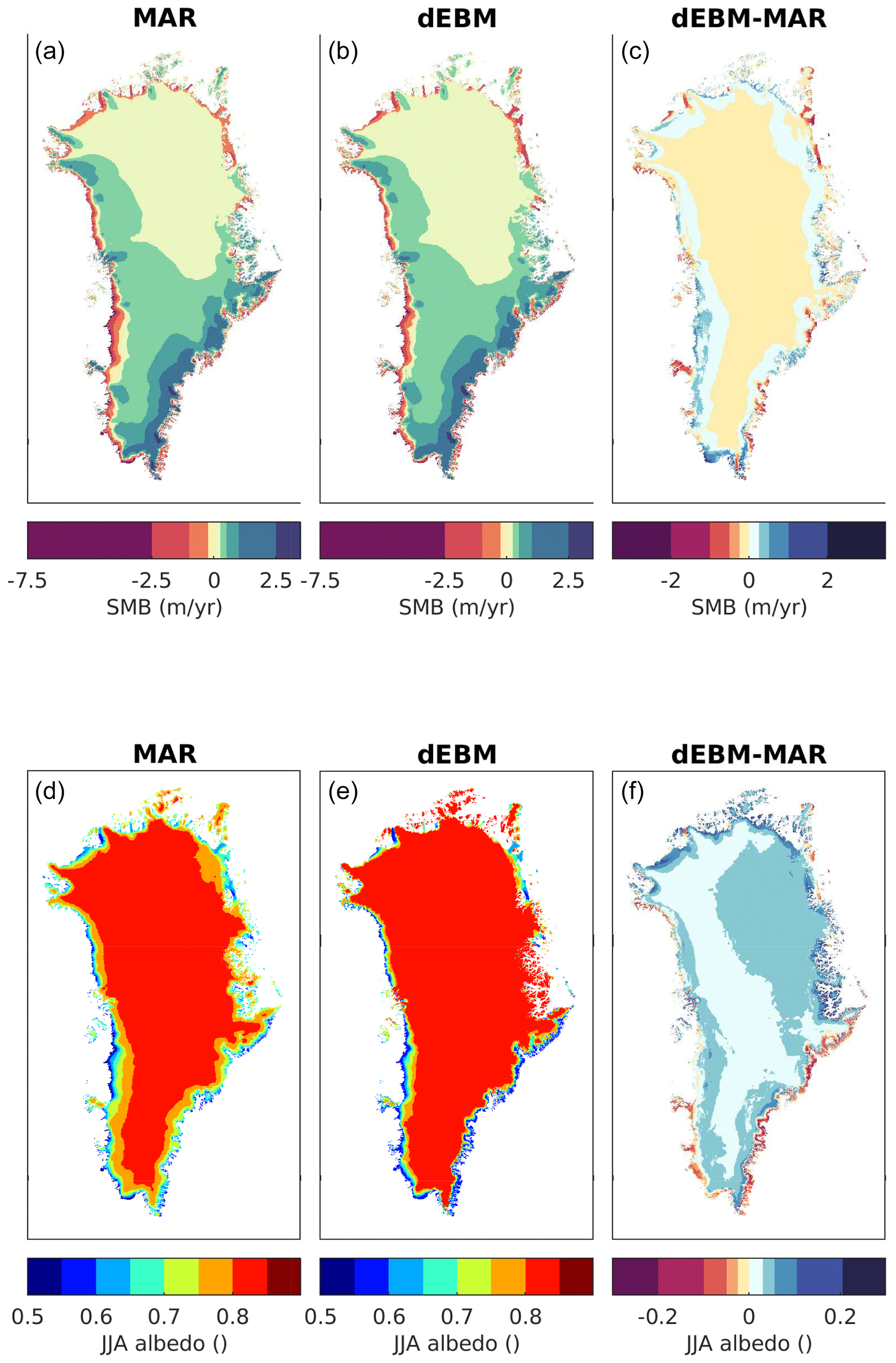
Figure 10 Comparison of multi-year (1980–1999) mean surface mass balance (a, b, c) and summer albedo (d, e, f) from experiments MAR_ERA (a, d) and dEBM_MAR,ERA (b, e) and differences between dEBM_MAR,ERA and MAR_ERA (c, f).

5 Sensitivity of the SMB to climate

5.1 Experimental design

We use dEBM to study the SMB of the Greenland Ice Sheet in a warm climate period of the past and in the warming climate of a future climate scenario. Both simulations have been conducted with the AWI Earth System Model, AWI-ESM (Sidorenko et al., 2015) at a horizontal resolution of approximately 1.85×1.85^∘ with 47 vertical levels (T63L47) in the atmosphere, and both experiments use an invariant present-day ice sheet geometry as boundary conditions.

Mid-Holocene simulation H6K. Due to a stronger-than-present axial tilt of the Earth (obliquity) the mid-Holocene (6000 years before present) was characterized by intensified summer insolation and consequently 2 to 3 ^∘C warmer summer temperatures over Greenland (Dahl-Jensen et al., 1998). The experiment H6K uses 200 years of monthly mean climate forcing from an equilibrated mid-Holocene simulation. The mid-Holocene simulation has been conducted using modified orbital parameters and greenhouse gas concentration following the PMIP protocols as defined in Otto-Bliesner et al. (2017).

The 1850 to 2099 simulation Industrial. The experiment Industrial uses 250 years of monthly forcing from an experiment with changing boundary conditions, which is a combination of a historical simulation from 1850 to 2005 and a future projection forced according to a high-emission scenario (following the Representative Concentration Pathway RCP8.5; Taylor et al., 2012).

In the following we use the years 1850 to 1899 of the experiment Industrial as a reference period (“PI” hereafter) for both experiments which here serves as a surrogate for the preindustrial period.

Here the AWI-ESM forcing is downscaled to an equidistant 5 km grid in contrast to the 1 km grid used in the previous section.

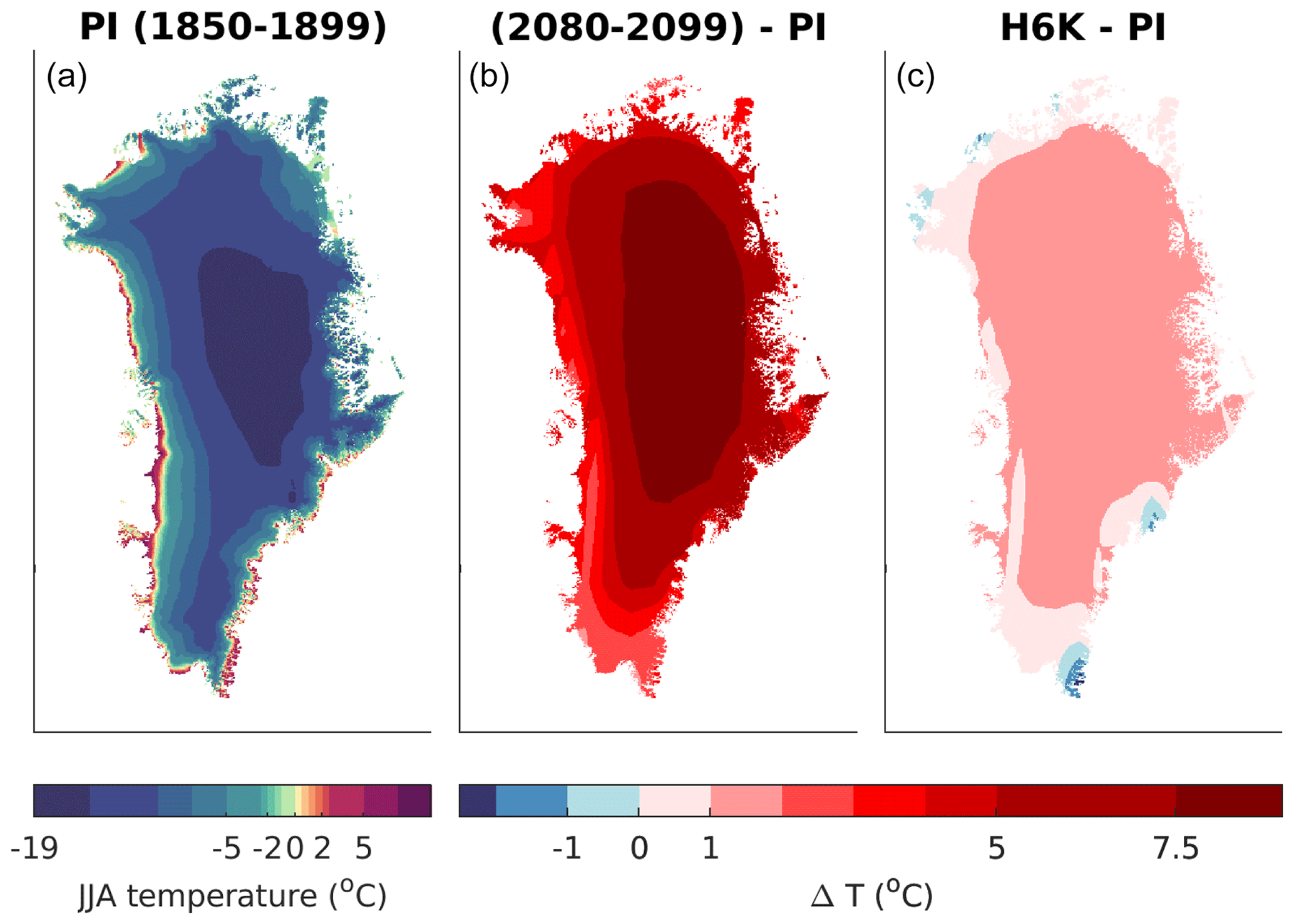
Figure 11 Mean summer 2 m temperature of the PI period (years 1850 to 1899) in the experiment Industrial (a) and anomalies of summer mean 2 m temperature with respect to PI of the Industrial experiment 2080 to 2099 period (b) and mean mid-Holocene (H6K) summer 2 m temperatures (c).

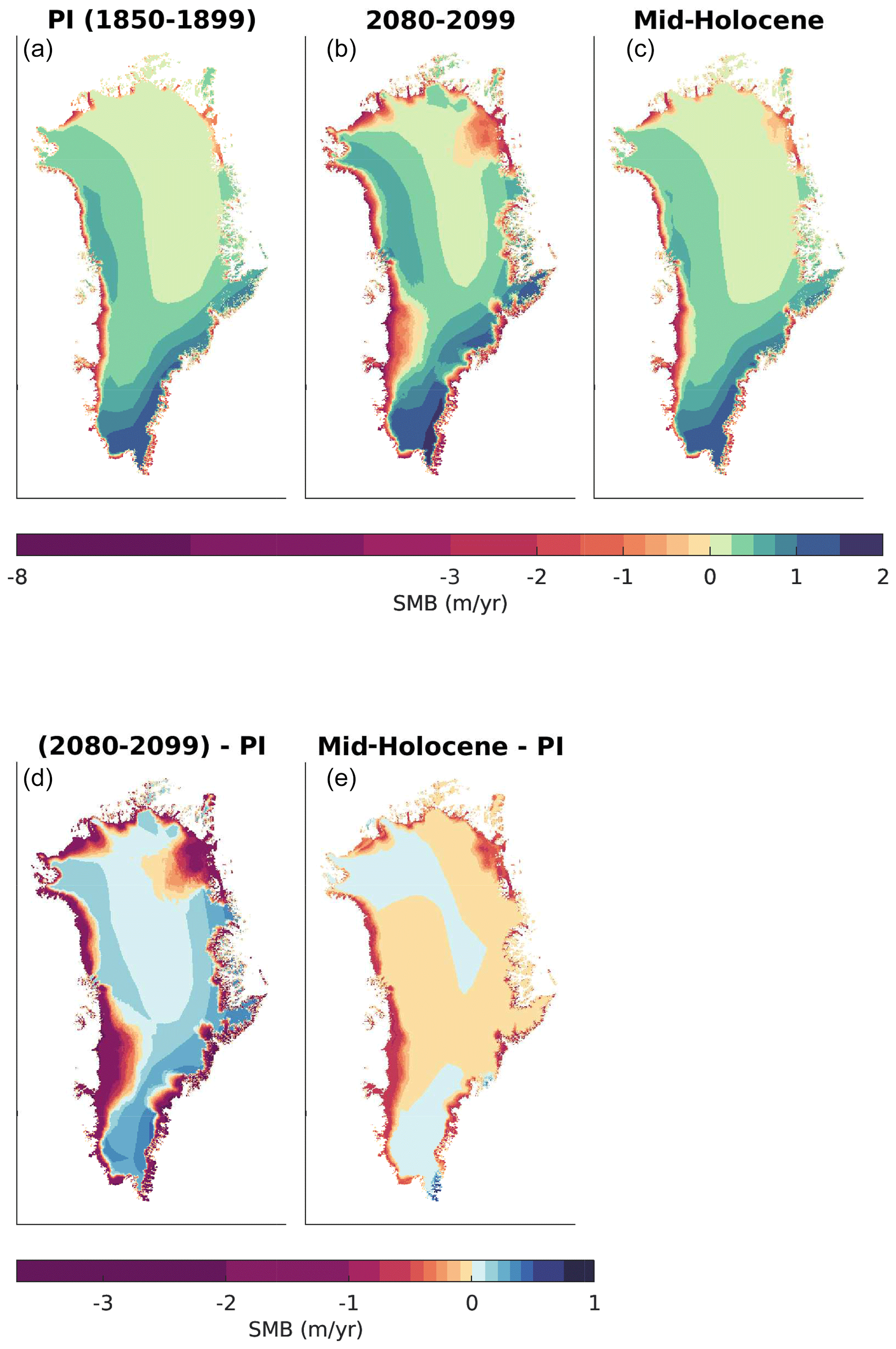
Figure 12 (a–c) Mean SMB of the experiment Industrial during the PI period (years 1850 to 1899, a), during the 2080 to 2099 period of the experiment Industrial (b) and mean SMB of experiment H6K. (d, e) SMB anomaly with respect to the PI period for the years 2080 to 2099 in the experiment Industrial (d) and for experiment H6K.

Figure 13 GrIS SMB time series from the experiment Industrial (red), experiment H6K (blue) and experiment MAR_ERA (black, Sect. 4). Fine lines show yearly accumulated values, and bold lines represent respective 5-year moving means.

5.2 Experiments H6K and Industrial

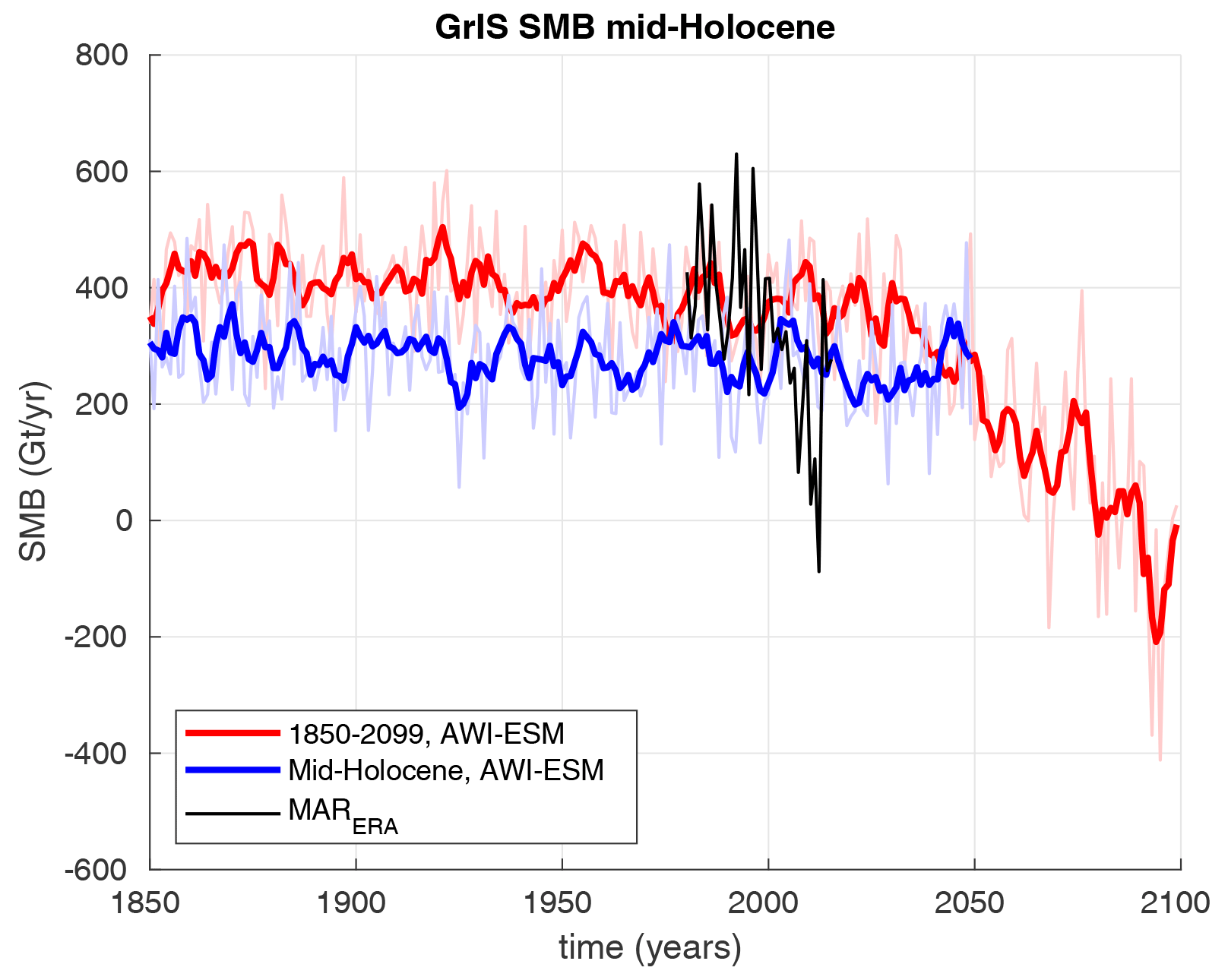
Compared to the PI period of the experiment Industrial, the climate of experiment H6K is characterized by stronger insolation and higher air temperatures over Greenland in summer (Fig. 11). In the ablation zone summer air temperatures exceed PI temperatures by approximately 0.5–1 ^∘C (Fig. 11), which is somewhat lower than reconstructed temperatures (Dahl-Jensen et al., 1998). The experiment Industrial exhibits a strong warming in the 21st century with summer air temperatures at the ice sheet's margins rising by 3–5 ^∘C above late 19th century values (Fig. 11). In response to the warmer climate of experiment H6K, dEBM simulates intensified melting and generally slightly extended ablation areas (Fig. 12), which in total decrease the mean SMB of the entire ice sheet by more than 100 Gt (Fig. 13). The transient climate of the experiment Industrial yields only a minor trend in SMB throughout the 20th century and starts to decrease substantially in the first half of the 21st century. By the end of the simulation SMB has decreased by more than 500 Gt, and the total SMB of the GrIS has changed its sign to negative. In particular in the west and northeast the ablation zone is no longer restricted to the margins but extends to the interior ice sheet (Fig. 12). The intensified melting is to some degree compensated for by higher accumulation rates. Simulated SMB around the end of the 20th century agrees well with the MAR simulation. The climate model however does not reproduce the extreme Greenland blocking in the 2005–2015 period, which is a common problem in global climate models (Hanna et al., 2018). Accordingly the interannual variations in SMB of recent decades are underestimated, and the simulated negative trend in SMB may be delayed.

5.3 Analysis of the temperature–melt relation

Local observations from Greenland reveal a linear relation between positive-degree days (PDD) and surface melt scaling with so-called degree day factors. This linear relationship is the basis of many empirical models (e.g., Reeh, 1991). For ice sheet applications degree day factors are commonly chosen to be DDF_ice≈ 8 mm (K d)⁻¹ and DDF_snow≈3 mm (K d)⁻¹ for snow and ice, respectively (Lefebre et al., 2002; Huybrechts et al., 1991). We now investigate the sensitivity of this relation between temperature and melt under different climates. For this purpose we separately integrate total simulated annual melt rates, positive-degree days and the temperature-independent terms of the surface energy balance (Eq. 5) $(\mathrm{1}-A)\mathrm{SW}\downarrow +b$ over two surface types. Here we do not distinguish between snow and ice but classify all local monthly melt rates ME of a given year into two subsets: ME_ws where the SurfaceType is equal to WetSnow and ME_ns,ds where SurfaceType is not equal to WetSnow. Analogously we analyze positive-degree days and the temperature-independent terms of Eq. (5) $(\mathrm{1}-A)\mathrm{SW}\downarrow +b$ in respective subsets of yearly output. Based on our dEBM simulations, we then infer degree day factors DDF_ws and DDF_ns,ds as in Krebs-Kanzow et al. (2018a) according to

$$\begin{array}{}\text{(16)}& \begin{array}{rl}{\mathrm{DDF}}_{\mathrm{ws}}& ={\displaystyle \frac{\sum {\mathrm{ME}}_{\mathrm{ws}}}{\sum {\mathrm{PDD}}_{\mathrm{ws}}}}\\ {\mathrm{DDF}}_{\mathrm{ns},\mathrm{ds}}& ={\displaystyle \frac{\sum {\mathrm{ME}}_{\mathrm{ns},\mathrm{ds}}}{\sum {\mathrm{PDD}}_{\mathrm{ns},\mathrm{ds}}}},\end{array}\end{array}$$

which represent an annual mean of all local degree day factors weighted by the melt rate (Fig. 14). Despite the inconsistency in the classification of surface types, we find a general agreement with the empirical parameters with ${\stackrel{\mathrm{‾}}{\mathrm{DDF}}}_{\mathrm{ws}}=\mathrm{8.7}$ mm (K d)⁻¹ and ${\stackrel{\mathrm{‾}}{\mathrm{DDF}}}_{\mathrm{ns},\mathrm{ds}}$ = 2.1 mm (K d)⁻¹ averaged over the 1850 to 1999 period. Both DDF_ws and DDF_ns,ds are especially sensitive to the H6K background climate with mean degree day factors ${\stackrel{\mathrm{‾}}{\mathrm{DDF}}}_{\mathrm{ws}}=\mathrm{9.8}$ mm (K d)⁻¹ and ${\stackrel{\mathrm{‾}}{\mathrm{DDF}}}_{\mathrm{ns},\mathrm{ds}}=\mathrm{3.1}$ mm (K d)⁻¹. Sensitivity to the warming climate of the 21st century is less pronounced with both degree day factors increasing by ≈ 0.3 mm (K d)⁻¹ towards the end of the experiment Industrial. Comparison with the temperature-independent terms of the surface energy balance (Eq. 5) indicates a linear relation between degree day factors and temperature-independent energy fluxes. The effect of shortwave radiation is in fact implicitly temperature dependent as surface albedo of glaciated surfaces usually decreases when air temperature exceeds melting point. This temperature dependence is also included in some albedo parameterizations (Bougamont et al., 2005; Aoki et al., 2003) and to some degree also represented in the dEBM by distinguishing three surface types.

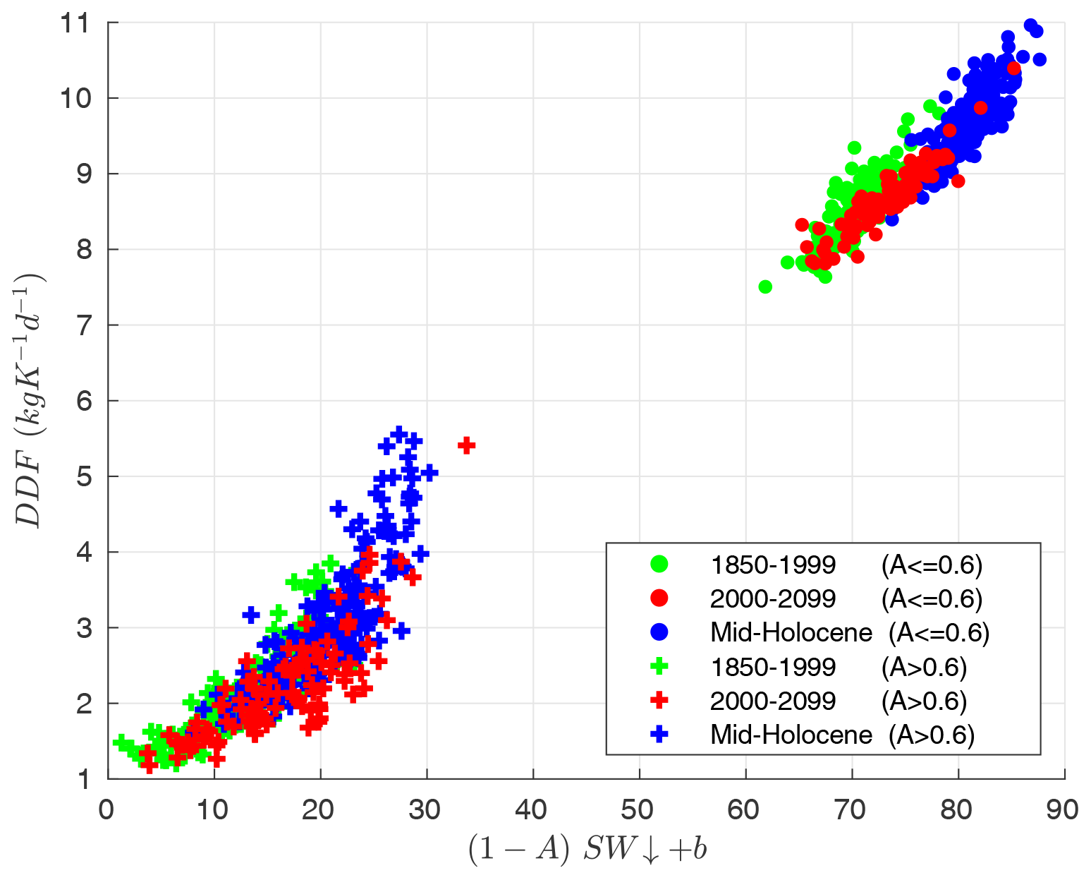
Figure 14 Degree day factors diagnosed from dEBM for the years 1850–1999 of the Industrial simulation (green), for the years 2000–2099 of the Industrial simulation (red) and for the 200 years of experiment H6K (blue) as a function of the temperature-independent terms in Eq. (5). Each circle (cross) represents a domain-wide annual mean of all monthly values for which SurfaceType is WetSnow (SurfaceType is not WetSnow) weighted by melt rate.

6 Summary and conclusions

The atmosphere influences the surface mass balance (SMB) of ice sheets on short temporal and small spatial scales, which induces long-term changes in continental ice volume in a changing climate. Usually, climate simulations that span more than a few centuries do not provide the required resolution to reliably predict the SMB, which implies the necessity to downscale climate forcing on long timescales. Here, we introduce the diurnal Energy Balance Model, dEBM, an SMB model of intermediate complexity. The dEBM is particularly suitable for Earth system modeling on multi-millennial timescales as model parameters are sufficiently general to remain applicable if atmospheric greenhouse gas concentration, or the seasonal and diurnal cycles, changes. The central concept of this model is the temporal downscaling that accounts for both submonthly variations in cloud cover and the diurnal melt–freeze cycle (Krebs-Kanzow et al., 2018b). This approach allows us to calculate SMB from monthly forcing with a monthly time step which reduces the computational cost substantially. In its Fortran version the actual dEBM code runs as sequential code on one core. After interpolation to the target grid, it takes about 5 s to compute the SMB of 1 year for a configuration with 360 000 grid points on a CPU core (Xeon Broadwell CPU; E5-2697v4, 2.3 GHz). A MATLAB version of the model simulates the 1979–2016 SMB of the GrIS at 1 km resolution (approximately 4.8 million grid points) in approximately 30 min on a Linux desktop PC. Requiring only monthly forcing also provides for an uncomplicated interface, as monthly forcing is usually more accessible in case of completed transient climate simulations such as simulations of the CMIP5 project (Taylor et al., 2012).

The model is physically plausible, as optimal parameters, calibrated to SMB observations from the GrIS, remain well within observational constraints.

The presented version agrees better with observations than an earlier version that already has, considering its simplicity, demonstrated a good skill to simulate the SMB of the GrIS (GrSMBMIP; Fettweis et al., 2020). The main progress in this new dEBM version is that atmospheric emissivity is no longer parameterized but is now diagnosed from the atmospheric forcing. Since Zolles and Born (2019) have demonstrated a strong sensitivity, the explicit inclusion of longwave radiation improves the computed SMB for a broad spectrum of climate stages ranging from glacial to future climate projections with strong radiative forcing. The dEBM compares well with simulated SMB from the complex regional climate model MAR (Fettweis et al., 2020) and exhibits an overall good agreement with local and integral observation and also reproduces individual extreme melt seasons of the last decades.

The dEBM does not downscale precipitation but interpolates precipitation forcing. A comparison of two dEBM simulations, which only differ in precipitation forcing, either originating from the ERA-Interim (Dee et al., 2011) reanalysis or from the regional climate model MAR, indicates that the coarser resolution of the reanalysis data induces a systematic bias in precipitation over Greenland. Coarse-resolution precipitation forcing represents a general source of error, but this is unlikely to affect the relative change of SMB in response to climate variations.

Furthermore, we have used dEBM in combination with two climate simulations from the global climate model AWI-ESM: a simulation of the mid-Holocene warm period and a transient global warming scenario which covers the period from 1850 to 2099. Both simulations exhibit warmer-than-present temperatures over the GrIS; the first one due to intensified summer insolation and the second one due to rising greenhouse gas concentration. In line with Plach et al. (2018) and van de Berg et al. (2011), the sensitivity of surface melt to air temperature increases by more than 10 % in the mid-Holocene experiment. In contrast, the temperature–melt relation barely changes during the global warming scenario. Hence, empirical temperature-based SMB methods like the commonly used PDD method might be applicable for the next decades but are not reliable on millennial timescales or outside of Greenland.

Naturally, the reduced complexity and the monthly time step of our model entail limitations. The comparison with MAR simulations reveals that the beginning and the end of the melt season is not truthfully simulated. In Greenland, under present-day climate these errors mostly cancel out but may also impair the representation of interannual variability. On orbital timescales, however, the melt season may be shorter or shifted in time, which may result in systematic errors over extended periods. In principle, these errors could be reduced or assessed by testing different time step schemes. Also owing to the monthly time step, dEBM may not reliably simulate the transition between dry and wet snow, where submonthly variability is usually strong (Fausto et al., 2011) and substantial surface melt may happen during short-lived warm spells. Furthermore, the model does not consider any processes within the snow column and relies on a simplistic albedo scheme, which may also impair the skill of the model near the upper boundary of the melt region or in regions with high accumulation rates. For these reasons the dEBM may not be well suited for small-scale applications outside of the main ablation zone, and it remains unclear whether this SMB model can be applied to individual glaciers or ice caps. In the context of long-term Earth system modeling, however, these shortcomings are unlikely to affect the sensitivity of the SMB to long-term climate change on the whole and probably are outweighed by uncertainties in climate forcing and boundary conditions.

Nevertheless, some extensions and modifications might be considered, depending on the problem and the region of interest. In coastal regions, the constant temperature sensitivity of the turbulent heat flux might be replaced by a function of wind speed. Further improvements might focus on the heat flux to the ground, the representation of liquid water storage in the snow column, a shorter time step and a downscaling algorithm for precipitation to reproduce better topographically steered precipitation. Furthermore, one might prescribe a background bare-ice albedo to account for regional darkening due to dust deposition or microbial activity (Wientjes et al., 2011; Cook et al., 2020).

As a natural next step we intend to test the dEBM in the framework of the coupled AWI-ESM Earth system model (Gierz et al., 2020) to study glacial–interglacial timescales. Furthermore, dEBM can be used as a diagnostic for climate simulations based on fixed ice sheet geometries or coupled to an ice sheet model using forcing derived from climate models and observation as in Niu et al. (2019). Overall, dEBM captures the essential physics which drive SMB variations on long timescales. We envision this intermediate-complexity model to be a low-cost alternative wherever dynamical downscaling with regional climate models is not feasible.

Appendix A

Table A1 Variables used in the dEBM.

Armstrong and Brun (2008)Robinson et al. (2010)Orvig (1954)Krebs-Kanzow et al. (2018b)

Table A2 Physical and empirical parameters used in this paper.