the Creative Commons Attribution 4.0 License.
the Creative Commons Attribution 4.0 License.
 | 21 Apr 2021
A new automatic approach for extracting glacier centerlines based on Euclidean allocation
Xiaojun Yao
Hongyu Duan
Shiyin Liu
Wanqin Guo
Meiping Sun
Dazhi Li
Glacier centerlines are crucial input for many glaciological applications. From the morphological perspective, we proposed a new automatic method to derive glacier centerlines, which is based on the Euclidean allocation and the terrain characteristics of glacier surface. In the algorithm, all glaciers are logically classified as three types including simple glacier, simple compound glacier, and complex glacier, with corresponding process ranges from simple to complex. The process for extracting centerlines of glaciers introduces auxiliary reference lines and follows the setting of not passing through bare rock. The program of automatic extraction of glacier centerlines was implemented in Python and only required the glacier boundary and digital elevation model (DEM) as input. Application of this method to 48 571 glaciers in the second Chinese glacier inventory automatically yielded the corresponding glacier centerlines with an average computing time of 20.96 s, a success rate of 100 % and a comprehensive accuracy of 94.34 %. A comparison of the longest length of glaciers to the corresponding glaciers in the Randolph Glacier Inventory v6.0 revealed that our results were superior. Meanwhile, our final product provides more information about glacier length, such as the average length, and the longest length, the lengths in the accumulation and ablation regions of each glacier.
- Article
(18474 KB) - Full-text XML
-
Supplement
(62796 KB) - BibTeX
- EndNote


Glaciers are an important freshwater resource on earth and a vital part of the cryosphere (Muhuri et al., 2015). According to the Fifth Assessment Report (AR5, https://www.ipcc.ch/, last access: 17 April 2021) published by the Intergovernmental Panel on Climate Change (IPCC), there are 168 331 glaciers (including ice caps) in the world, with a total area of 726 258 km2 apart from ice sheets. Glaciers move towards lower altitude by gravity, which is the most obvious distinction between glacier and other natural ice bodies. The glacier flow lines are the motion trajectories of a glacier, and the main flow line is the longest flow trajectory of glacier ice. Due to the differences in the speed and moving direction of any point at the surface or inside the glacier, the calculation of the main flow line of glaciers requires coherent velocity field data, which are difficult to obtain on the global or regional scale (McNabb et al., 2017). Therefore, some concepts such as the glacier axis and the glacier centerlines were proposed (Le Bris and Paul, 2013; Kienholz et al., 2014; Machguth and Huss, 2014). Glacier centerlines are the central lines close to main flow lines of glaciers, which can be acquired based on glacier axis and be used to simulate the glacier flow line.
As an important model parameter, the glacier centerline can be used to determine the change of glacier length (Leclercq et al., 2012a; Nuth et al., 2013), analyze the velocity field (Heid and Kääb, 2012; Melkonian et al., 2017), estimate the glacier ice volume (Li et al., 2012; Linsbauer et al., 2012) and develop one-dimensional glacier models (Oerlemans, 1997; Sugiyama et al., 2007). Meanwhile, the length of the longest glacier centerline is one of the key determinants of glacier geometry and an important parameter of a glacier inventory (Paul et al., 2009; Leclercq et al., 2012b). The length and area of the glacier can also be used to estimate the large-scale glacier ice volume (Zhang and Han, 2016; Gao et al., 2018). The length change at the terminus of a glacier can directly reflect the state of motion, e.g., glacier recession, glacier advance or surging (Gao et al., 2019). Winsvold et al. (2014) analyzed the changes of glacier area and length in Norway, using glacier inventories derived from Landsat TM/ETM+ images and digital topographic maps. Herla et al. (2017) explored the relationship between the geometry and length of glaciers in the Austrian Alps based on a third-order linear glacier length model. Leclercq and Oerlemans (2012), Leclercq et al. (2014) reconstructed annual averaged surface temperatures in the past 400 years on hemispherical and global scales from glacier length fluctuations. These studies indicated that both the extraction of contemporary glacier length and the reconstruction of historical glacier length require more accurate extraction methods of glacier flow lines.
In order to obtain the length of glaciers, some automatic or semi-automatic methods were proposed in recent years. Schiefer et al. (2008) extracted the longest flow path on the ice surface based on a hydrological model, which was generally 10 % to 15 % larger than the glacier length. Le Bris and Paul (2013) accomplished the automatic extraction of flow lines from the highest point to the terminus of a glacier based on the concept of glacier axis, with a verification accuracy of 85 %. Unfortunately, the branches of glacier centerlines have not been extracted, and the length is not necessarily the maximum for huge or complex glaciers (Paul et al., 2009). Machguth and Huss (2014) proposed an extraction method of glacier length based on the slope and width of a glacier with a success rate of 95 %–98 %; however the branches of glacier centerlines could not be extracted either. Kienholz et al. (2014) applied the grid–least-cost route approach to the automatic extraction of glacier flow lines, having an automation degree of 87.8 % with additional manual intervention. Yao et al. (2015) proposed the semi-automatic method of extraction glacier centerlines based on Euclidean allocation theory, which required the expertise and experiences for composite valley glaciers and ice caps. So, the current biggest challenge is still the implementation of automated extraction of the glacier centerline and the acquirement of more information about glacier length. The aims of this study are to design an algorithm to (i) automatically generate centerlines for the main body of each glacier and its branches; (ii) automatically calculate the longest length, average length, length of the accumulation region and length of the ablation region of each glacier, along with corresponding polylines; and (iii) improve the degree of automation as much as possible on the premise of ensuring the accuracy of glacier centerlines.
The glacier dataset used in this study is the Second Chinese Glacier Inventory (SCGI) released by the National Tibetan Plateau Data Center (http://westdc.westgis.ac.cn/data, last access: 17 April 2021), which has been approved by some organizations (e.g., WGMS, GLIMS, NSIDC) and adopted in the Randolph Glacier Inventory (RGI) v6.0 (Guo et al., 2017). According to the SCGI (Fig. 1), there were 48 571 glaciers in China, with a total area of 51 766.08 km2, accounting for 7.1 % of the glacier area in the world except for the Antarctic and Greenland ice sheets (Liu et al., 2015). Due to the lack of an automatic method to calculate a glacier's length, there was no length property in the SCGI, and some subsequent studies have not made great breakthroughs (Yang et al., 2016; Ji et al., 2017).
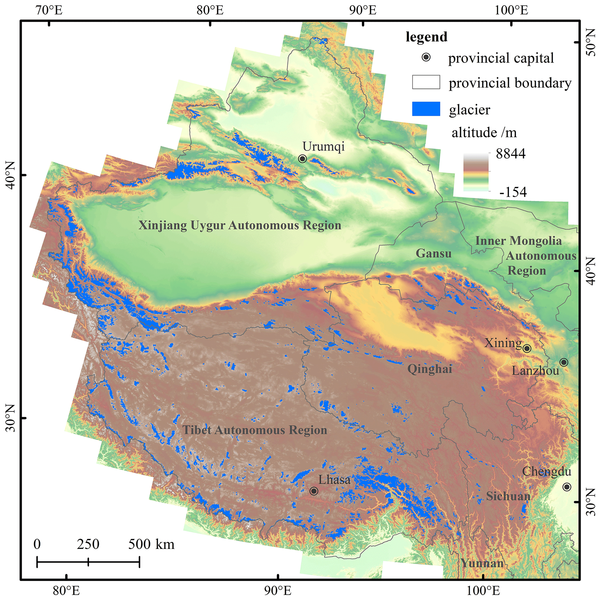
Figure 1The distribution of glaciers in China.
The SCGI was produced based on Landsat TM/ETM+ images and ASTER images in the period of 2004–2011 and SRTM v4.1 with a spatial resolution of 90 m (Liu et al., 2015). In this study, we selected SRTM1 DEM v3.0 (http://www2.jpl.nasa.gov/srtm, last access: 2 March 2013, with a spatial resolution of 30 m) (Farr et al., 2007) in consideration of its free access and higher data quality, which was used to identify division points on the glacier outlines, extract ridge lines in the coverage region of glaciers and generate the glacier centerlines. Additionally, we extracted glaciers in China from the RGI v6.0 provided by GLIMS (http://www.glims.org/RGI/, last access: 17 April 2021). There are 38 053 glaciers matching the graphic position of the SCGI. The field of Lmax of RGI v6.0 provides the length of the longest flow lines on the glacier surface, which was calculated with the algorithm proposed by Machguth and Huss (2014). For verifying the validity and accuracy of glacier centerlines, we compared the extracted longest length of glaciers with the value of Lmax in the RGI v6.0.
In order to implement the automatic extraction of glacier centerlines, we have designed a new set of algorithms. Relevant parameters and processing procedures are introduced as follows.
3.1 Model parameters
The code was written in Python and partially invoked the site package of ArcPy. The calculation of the glacier centerlines relies on two basic inputs: (i) glacier in the form of polygon with a unique value field and a projection coordinate system (unit: m) and (ii) DEM data having the spatial resolution and acquisition time close to the images used for a glacier inventory. We defined 11 adjustable parameters named ) (see Table 1), which were achieved by classifying a glacier polygon through a set of reasonable rules. The purpose is to improve the degree of automation and the accuracy. Three key parameters are described as
-
P3, the threshold of flow accumulation, to control the generation of auxiliary lines;
-
P6, the step size of searching the local highest points, to control the extraction of extremely high points;
-
P8, the grid cell size of Euclidean allocation, to improve the algorithm efficiency.
Table 1The description of adjustable parameters.
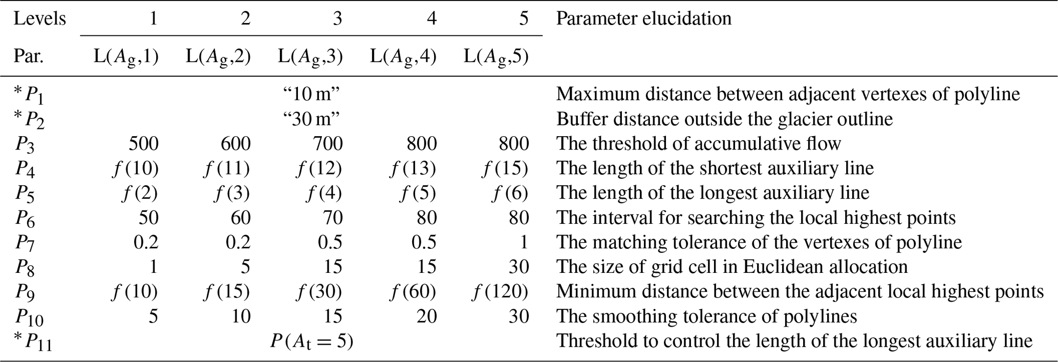
Note: the parameters with * are constant.
In the algorithm, the number of the local highest points is affected by the perimeter of the glacier (Pg). We took the given area (At) and the perimeter (Pt, Eq. 1) of the equilateral triangle corresponding to At as the grading threshold. According to the area (Ag) and the perimeter (Pg) of each glacier's outer boundary, all glaciers were divided into five levels (Eq. 2), which represented the five levels of a glacier polygon with a difference in Pg. The built-in parameters were set according to the different levels (Table 1). P4, P5 and P9 were controlled in proportion to the side length of the equilateral triangle corresponding to Pt. The proportional coefficient was T (Eq. 3). According to the actual situation of the repeated programming test, the empirical value of each parameter is given in Table 1.
where is the threshold (unit: km2) set of glacier area and denotes the corresponding levels of glaciers and is used as the index of array A.
3.2 Computation flow
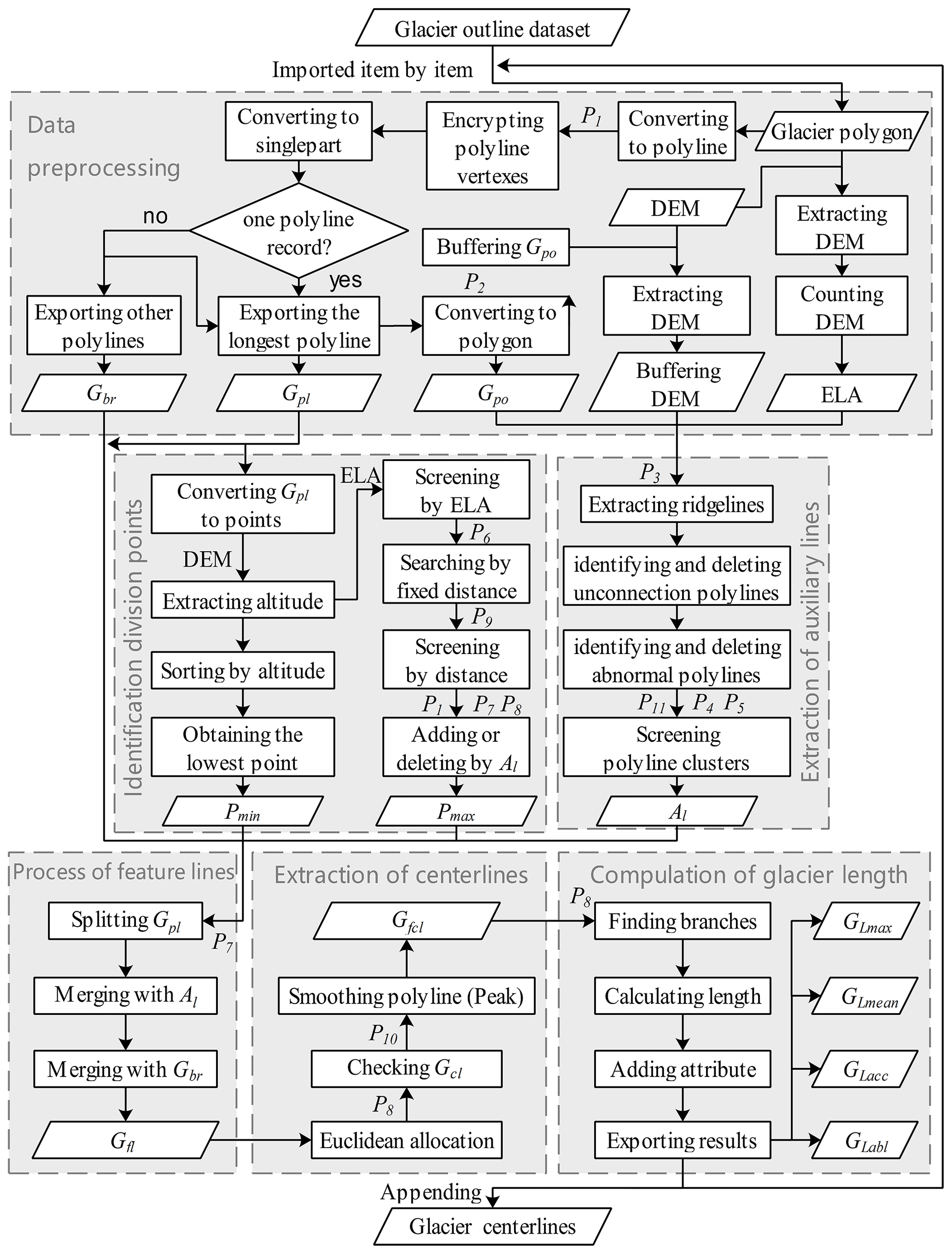
In this paper, glaciers were divided into three categories: simple glacier (extremely high point: single; auxiliary line: no; the area of bare rock: no), simple compound glacier (extremely high point: several; auxiliary line: no; the area of bare rock: no) and complex glacier (extremely high point: several; auxiliary line: yes; the area of bare rock: yes). Following the principle from simple to complex, the algorithm was composed of six main steps: data preprocessing, extraction of auxiliary lines, identification of division points, reconstruction of feature lines, extraction of centerlines and calculation of glacier length. The flow chart of the algorithm is illustrated in Fig. 2.
The automatic extraction of glacier centerlines in this study obeys the following rules: (i) the elevation of the local highest points must be higher than the equilibrium line altitude (ELA); (ii) a glacier has only one exit, which is the lowest point of the polyline of the glacier's outer boundary (Gpl); (iii) the auxiliary line only acts on the accumulation region of glacier; and (iv) the Gpl, auxiliary lines and bare rock region simultaneously serve as barrier lines to restrict the flow direction of the glacier centerlines.
3.3 Critical processes
3.3.1 Data preprocessing
The data preprocessing includes four parts: (i) checking the input data, (ii) pre-processing the glacier outlines, (iii) fine-tuning the built-in parameters and (iv) calculating the ELA of glaciers. First, the polygon of the glacier's outer boundary (Gpo), the polyline of glacier's outer boundary (Gpl) and the boundary of the bare rock in glacier (Gbr) were obtained by splitting the glacier outlines in the importing module. These temporary data would be used as the input parameters of other modules in the subsequent process. Secondly, the module exported the number of closed lines in glacier outlines Ag and Pg, which were used to determine the number of bare rocks on the glacier surface and the type and level of glaciers. Thirdly, according to the parameter-adjusting rules at the level of glaciers, 11 built-in parameters (see Table 1) were fine-tuned. Finally, the median elevation (Zmed) of each glacier aided by its DEM was computed, which was then used to estimate the ELA of each glacier. The schematic diagram of processing glacier outlines is shown in Fig. 3.

Figure 3The schematic of processing raw data (Gpo denotes the polygon of the glacier, Gpl denotes the polyline of the glacier's outer boundary and Gbr denotes the boundary of the bare rock in the glacier).
3.3.2 Extraction of auxiliary lines
For making glacier centerlines more reasonable, we introduced the auxiliary lines that represent the internal ridgelines of glaciers to intervene in the generation of centerline for the upper part of a glacier. The extraction of auxiliary lines included the extraction of ridgelines and post-processing. Based on the inverse terrain method, the extraction of ridgelines was easily accomplished by the workflow of hydrologic analysis. The post-processing was relatively complicated. The main reason was that the auxiliary lines were tree-like polylines starting from the upper boundary of the glacier. In principle, the mass flow in the location of the auxiliary lines on the glacier surface could be obviously blocking-up, which was equivalent to the ice divide. The preliminary ridgelines needed to be screened once more combined with a DEM by the traversal method. Determining the cluster of auxiliary lines was the main problem to be solved by the algorithm of this part. According to the designed algorithm, it could be divided into five parts in post-processing: (i) identifying and deleting the disconnected lines, (ii) identifying and deleting the abnormal lines, (iii) determining the members of line cluster, (iv) determining the longest length of line cluster and (v) screening the line clusters. The schematic diagram of extracting the auxiliary lines is shown in Fig. 4.
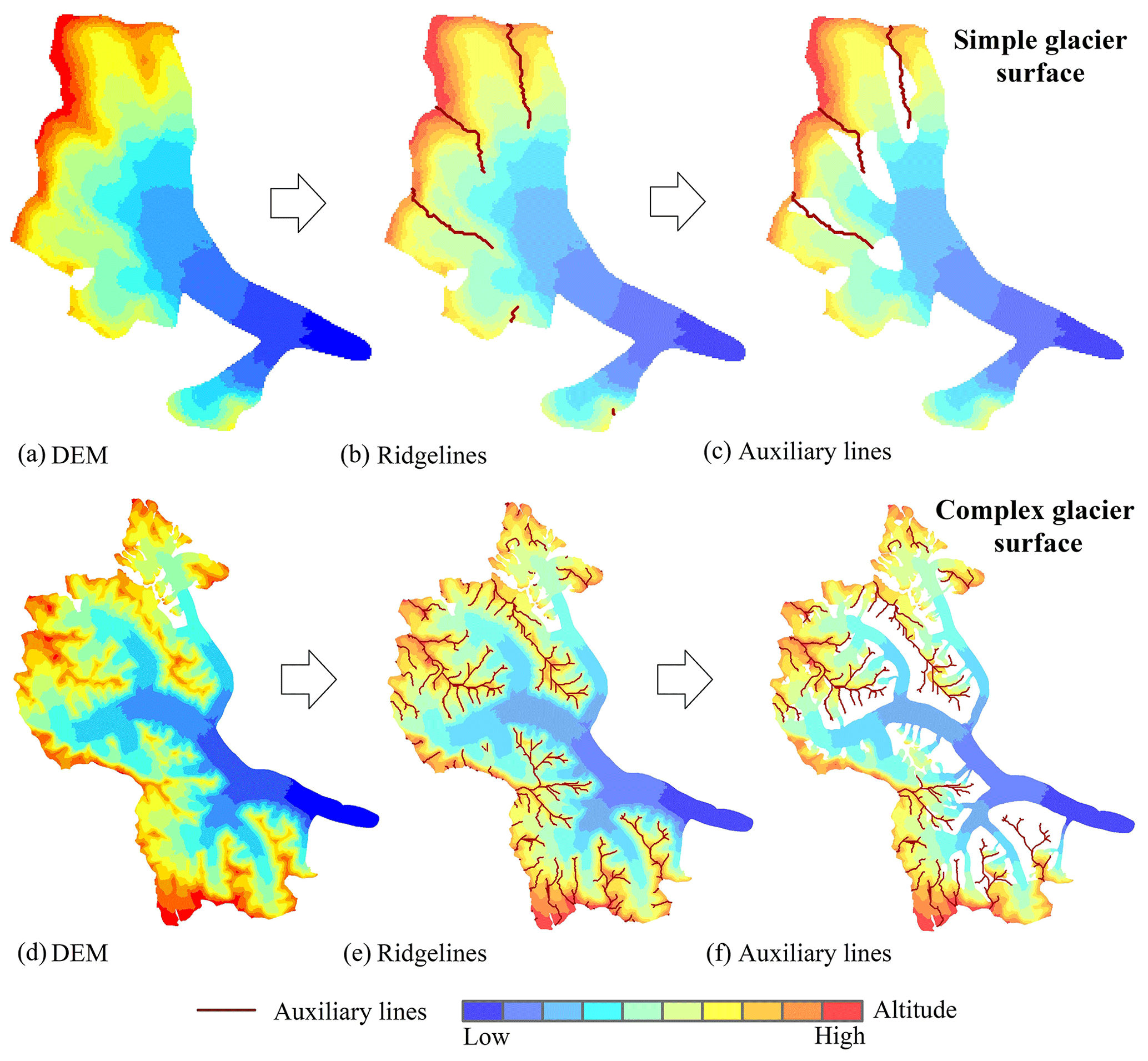
Figure 4The schematic of extracting auxiliary lines. Panels (a and d) demonstrate the digital elevation model (DEM) around the glacier. Panels (b and e) show the ridgelines in the region covered by the DEM. Panels (c and f) show the auxiliary lines in the glacier.
The automatically extracted ridgelines were often disconnected, so it was necessary to remove independent existence or unreasonable ridgelines using the auxiliary data such as DEM, ELA and Gpo by ergodic algorithms. Firstly, the ridgelines of the glacier surface (Ar) were obtained by clipping the ridge lines using Gpo. The set of all possible starting points of auxiliary lines was gained by intersecting Ar with Gpl. Then, the ridgeline clusters connected to each starting point were achieved and marked by traversing the point set. The number of auxiliary lines was initially determined. Lastly, the longest length of each auxiliary line was calculated by adopting the critical path algorithm. The final auxiliary lines (Al) were obtained by screening all auxiliary lines using the three parameters of P4, P5 and P11.
3.3.3 Identification of division points
The division points include the lowest point (Pmin) and the local highest point (Pmax). The ordered point set (h) was obtained after converting Gpl from a polyline to a point set and extracting the elevation for the point set. The method for obtaining Pmin was relatively simple, as shown in Eq. (4).
In comparison, the extraction of Pmax was more complicated. It was necessary to ensure the extraction of all possible branches of the centerlines and avoid the redundancy of branches. The algorithm could be divided into four steps: (i) obtaining the local highest point set (M′′) by filtering h (Eqs. 5 and 6) according to P6; (ii) removing the elements (Eq. 7) at an altitude lower than ELA from M′′; (iii) removing the elements (Eq. 8) of adjacent distance less than P9 from M′; and (vi) checking, deleting or adding some local highest points (Eq. 9) using the auxiliary lines to ensure that there was at least one local highest point among adjacent auxiliary lines.
3.3.4 Reconstruction of feature lines
Feature lines of glacier surface were used to express Gpl, Gbr, Al, Pmax, Pmin, and the intersection of Al and Gpl. The schematic diagram of merging the glacier surface features is illustrated in Fig. 5.
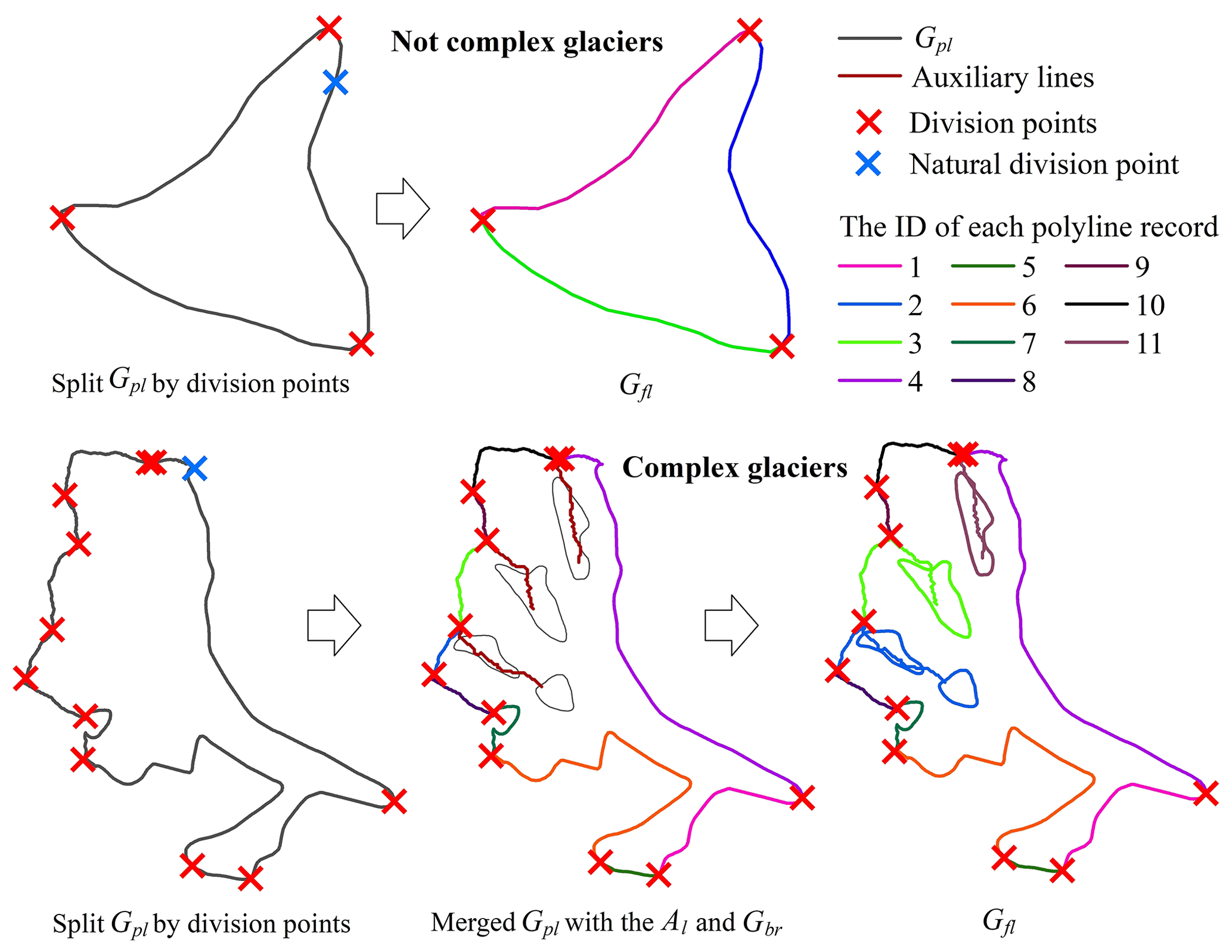
Figure 5The schematic of extracting the polyline features of glacier surface.
For simple glaciers and simple compound glaciers, it was only necessary to merge Pmax and Pmin into a vector file, then split Gpl and allocate one unique code for each polyline after converting it from multipart to single part. For a complex glacier, the processing method was composed of several steps. First of all, the Gpl split by division points needed to be combined with Gbr (if any) and Al (if any) into a vector file. After converting it from multipart to single part, the program would again allocate code for each polyline and remark it as Gsp1. Secondly, polyline records in Gsp1 were selected one by one with Al, and then the polyline records belonging to the same part in Gsp1 were merged, which was recorded as Gsp2. Thirdly, Gedge was exported by selecting Gsp2 using Gpl, and Galone was exported after switching selection, which represented the bare rock region that still existed independently after merging the glacier outlines with the auxiliary lines. Finally, adopting the proximity algorithm, each element (if any) in Galone was processed in turn with Gedge. Specifically, it needed three steps. (i) The vertex set E (Eq. 10) of Gedge and the vertex set U (Eq. 11) of Galone were obtained. (ii) The pairs of polylines (Eq. 12) matched by serial number were calculated, and the corresponding marks in Gsp2 were made. (iii) The feature lines (Gfl) of glacier surface were reconstructed by merging the same marks in Gsp2.
3.3.5 Extraction of glacier centerlines
Original glacier centerlines (Gcl) were achieved with the function of Euclidean allocation in ArcPy, which needed the input of Gfl and set the value of P8. Firstly, the feature lines (Gfl) after automatically deriving by the program are input, and the function of Euclidean allocation in ArcPy is called to generate the division glacier surface. Then the common edges between regions on the dividing glacier surface are identified. Finally, the common edges are automatically checked and processed to obtain Gcl. The final glacier centerlines (Gfcl) were obtained by processing Gcl with the Peak algorithm, after setting the tolerance for smoothing polylines (P10). The schematic diagram of extracting Gfcl and the longest length of glaciers (GLmax) is shown in Fig. 6.
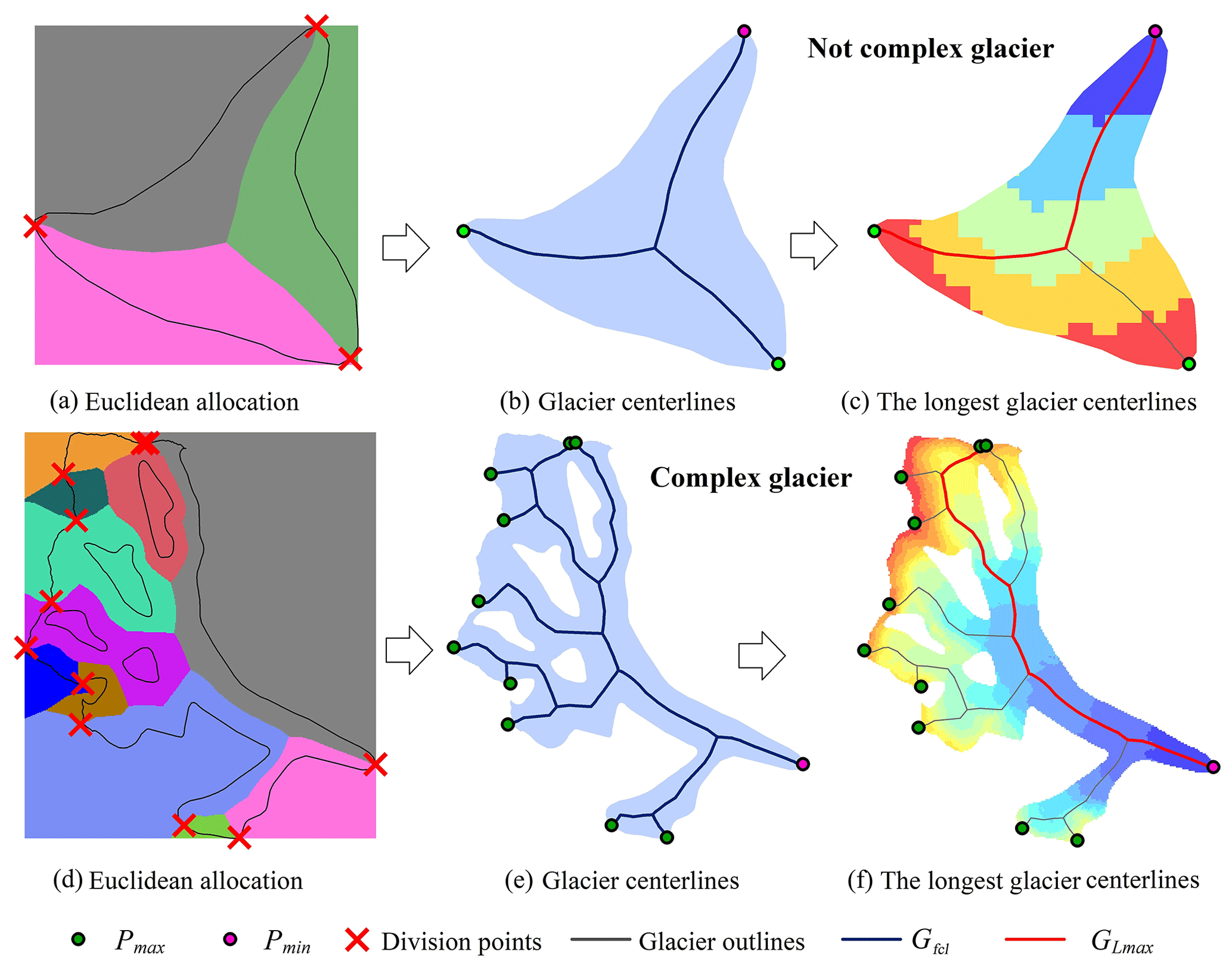
Figure 6The schematic of extracting centerlines and the longest centerline of the glacier. Panels (a and d) show the results after executing the European allocation, and the different colors represent the regions which have the shortest distance to the corresponding edges of the glacier. Panels (b and e) represent the centerlines(Gfcl), the local highest point (Pmax) and the lowest point (Pmin) of the glacier. Panels (c and f) demonstrate the longest centerline (GLmax) of the glacier, and the background is the digital elevation model with the graduated red (high) – blue (low) color.
3.3.6 Calculation of glacier length
The final code of the Gfcl was determined by Pmin after Gfcl being converted from multipart to single part and was given in a unified format. Then all branches of glacier centerlines and glacier length were achieved using algorithm (Fig. 7) similar to the critical path. This work consisted of four steps. (i) The polyline set of Gfcl was recorded as C (Eq. 13), and then the sets of polyline length (L) and polyline endpoint (S) (Eq. 13) were obtained. (ii) The initial search point (B) (Eq. 14), the end of the glacier centerline, was determined by the coordinates of Pmin based on the above steps. The common endpoint set (N) (Eq. 14) with the next parts of glacier centerlines was obtained, and then the polyline code corresponding to B was recorded. (iii) Each element in N was used as a new starting point for the search (B′) (Eq. 15), which was used to get the common endpoint set (N′) (Eq. 15) with the next parts of the glacier centerlines. The coding of the corresponding polyline set of each glacier branch was recorded separately, and (vi) the above process continued until all branches of the glacier centerline trace back to its corresponding Pmax (Eq. 16).
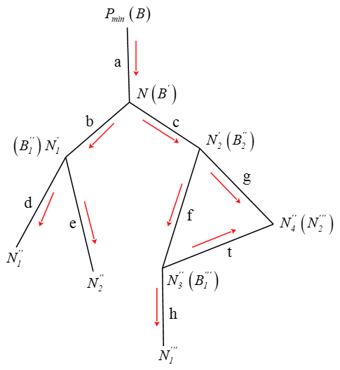
Figure 7The schematic of calculating glacier length (the red arrow represents the search direction of the branches of the glacier centerline).
The length of each branch of the glacier centerlines was counted. The average length (Eq. 17) of all branches was named the average length of a glacier (GLmean). The longest length (Eq. 18) of all branches was named the longest length of a glacier (GLmax). In addition, the part above ELA in GLmax was regarded as the accumulation region length (GLacc) of a glacier, and the part of GLmax with altitude lower than ELA was regarded as the ablation region length (GLabl) of a glacier. Finally, the corresponding vector data were generated and some attributes including the corresponding polyline code, glacier code and the value of glacier length were added.
4.1 Methods of quality analysis
Here, we used the SCGI as the test data to run the designed program, including 48 571 glaciers. The extraction results of some typical examples of glaciers (from simple to complex) are presented in Fig. 8. The accuracy of glacier centerlines was evaluated based on a random verification method in this study. All glaciers (total quantity: NG) corresponding to the samples were obtained and arranged in ascending order of the area. Specifically, 100 random integers were generated in the set of [0, NG). Glaciers with a corresponding serial number were exported as samples. After the visual inspection, the accuracy evaluation was conducted based on the following statistical analysis.
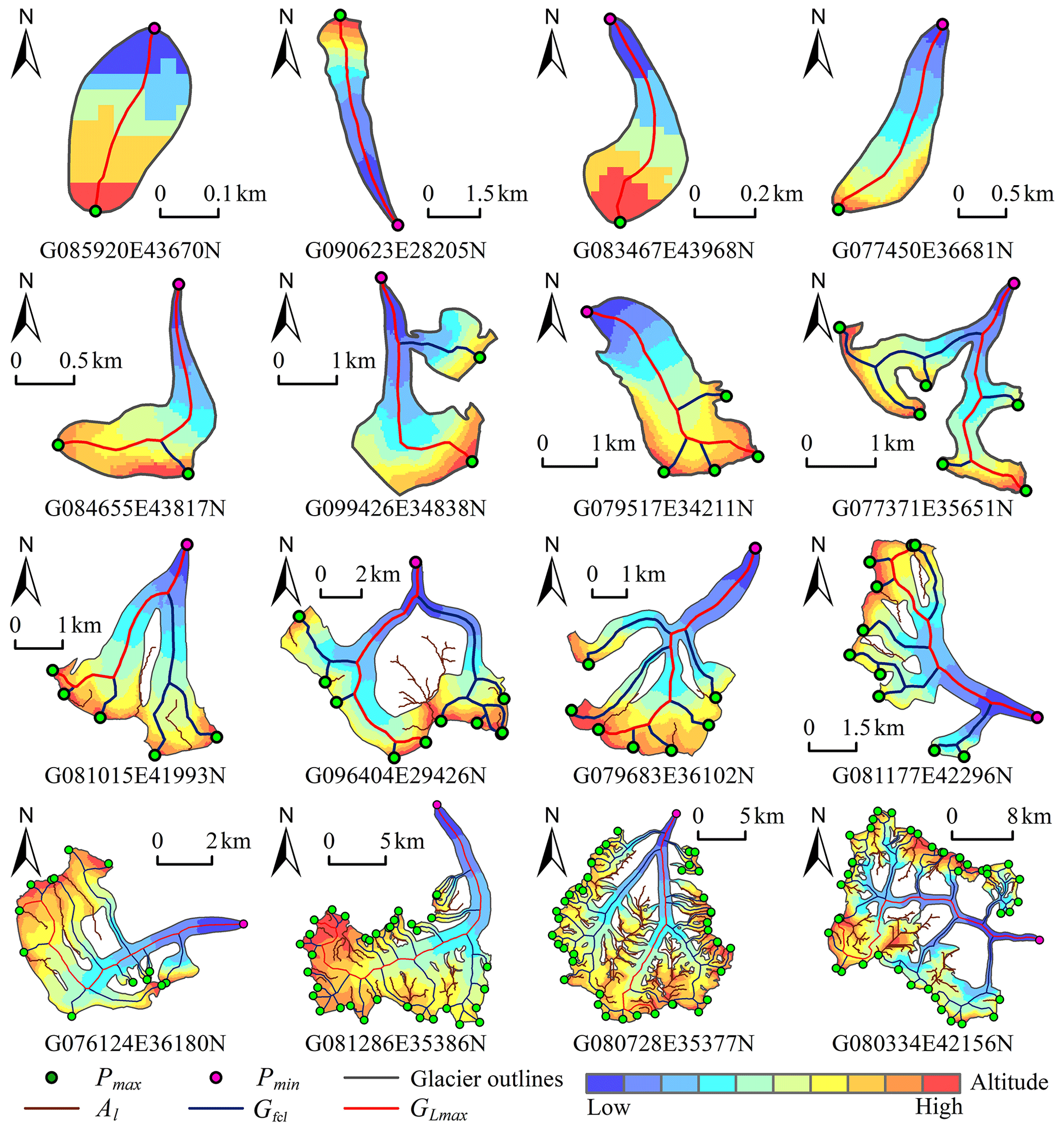
Figure 8The centerlines for some typical glaciers (Pmax and Pmin denote the local highest point and lowest point in the boundary of the glacier, respectively; Al denotes the auxiliary lines; Gfcl and GLmax denote the centerlines and the longest centerline of the glacier).
Firstly, 100 glaciers were randomly selected from the glacier dataset as samples to obtain a verification accuracy (R1) (Eq. 19). Secondly, each level of glacier was separately taken as the total (NT), and 100 glaciers were randomly selected. There were five samples for five levels, which were used to calculate a verification accuracy (R2) (Eq. 20) by taking the number proportion of each glacier level as the weight. Then, 100 glaciers with the largest, middle and smallest areas were selected separately as samples. The verification accuracy (R3) (Eq. 21) was derived using as the allocation proportion of weight. Finally, the average value of R1, R2 and R3 was used as the comprehensive accuracy (R) (Eq. 22). Among them, Si represented the verification accuracy of the ith sample ().
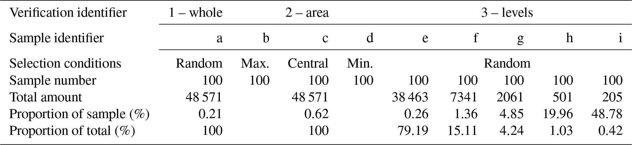
4.2 Sample selection and assessment criteria
Visual inspection in combination with satellite images and topographic maps is the most direct evaluation method for extraction results. Using 48 571 glaciers in China as the test data, nine samples of 900 glaciers were selected for three verifications according to the evaluation method defined in Sect. 4.1. The samples used for verification and relative information are given in Table 2.
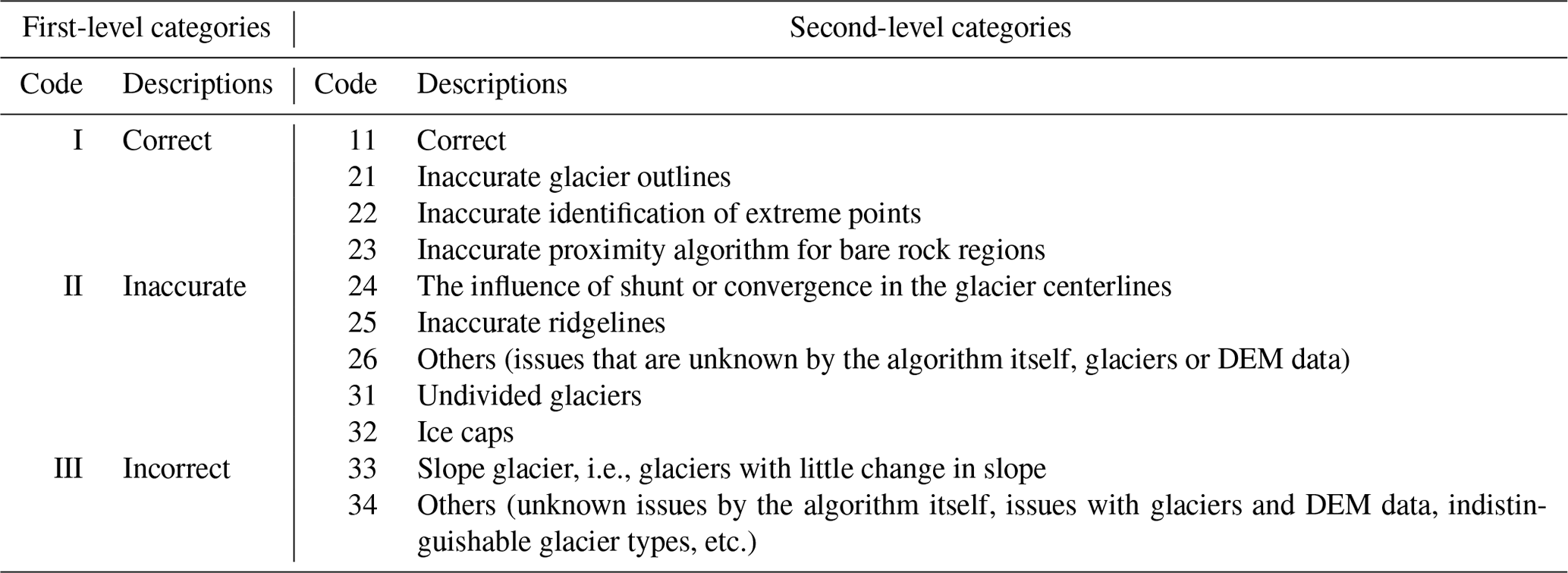
Considering the possible defaults of the input data, we set some standards of accuracy evaluation (Table 3). The first level includes three categories: correct (I), inaccurate (II) and incorrect (III). The secondary categories were divided into 11 categories according to probable causes, among which the inaccurate causes and incorrect causes were subclassified as six types and four types, respectively. Type II mostly involves glaciers with accurate GLmax but missing, redundant or unreasonable branches of glacier centerlines. When calculating the comprehensive accuracy, categories I and II were regarded as correct, and only category III was considered incorrect.
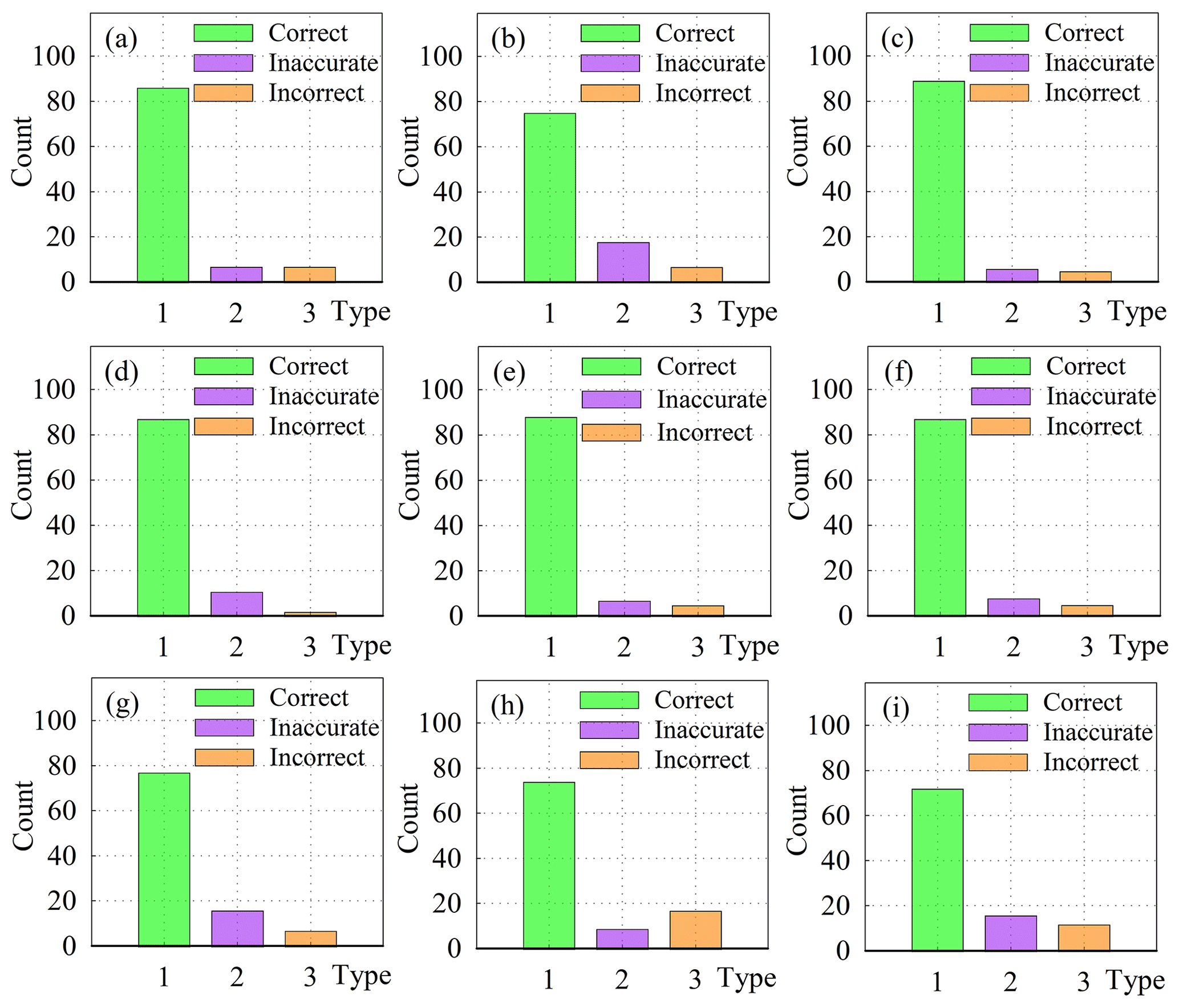
Figure 9The statistical chart of evaluating results according to the first-level categories.
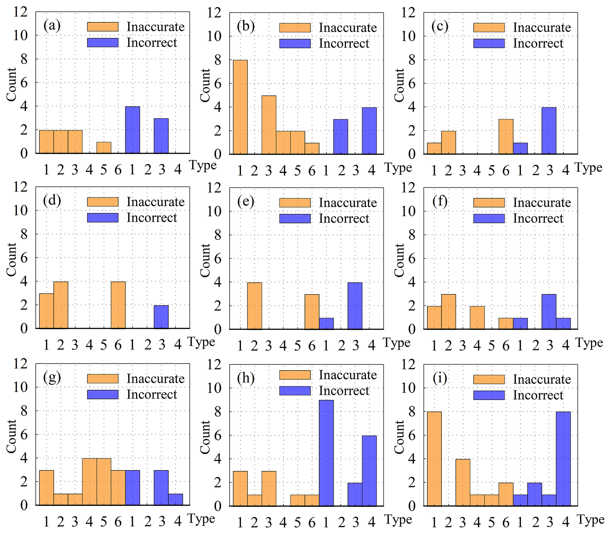
Figure 10The statistical chart of evaluating results according to the second-level categories.
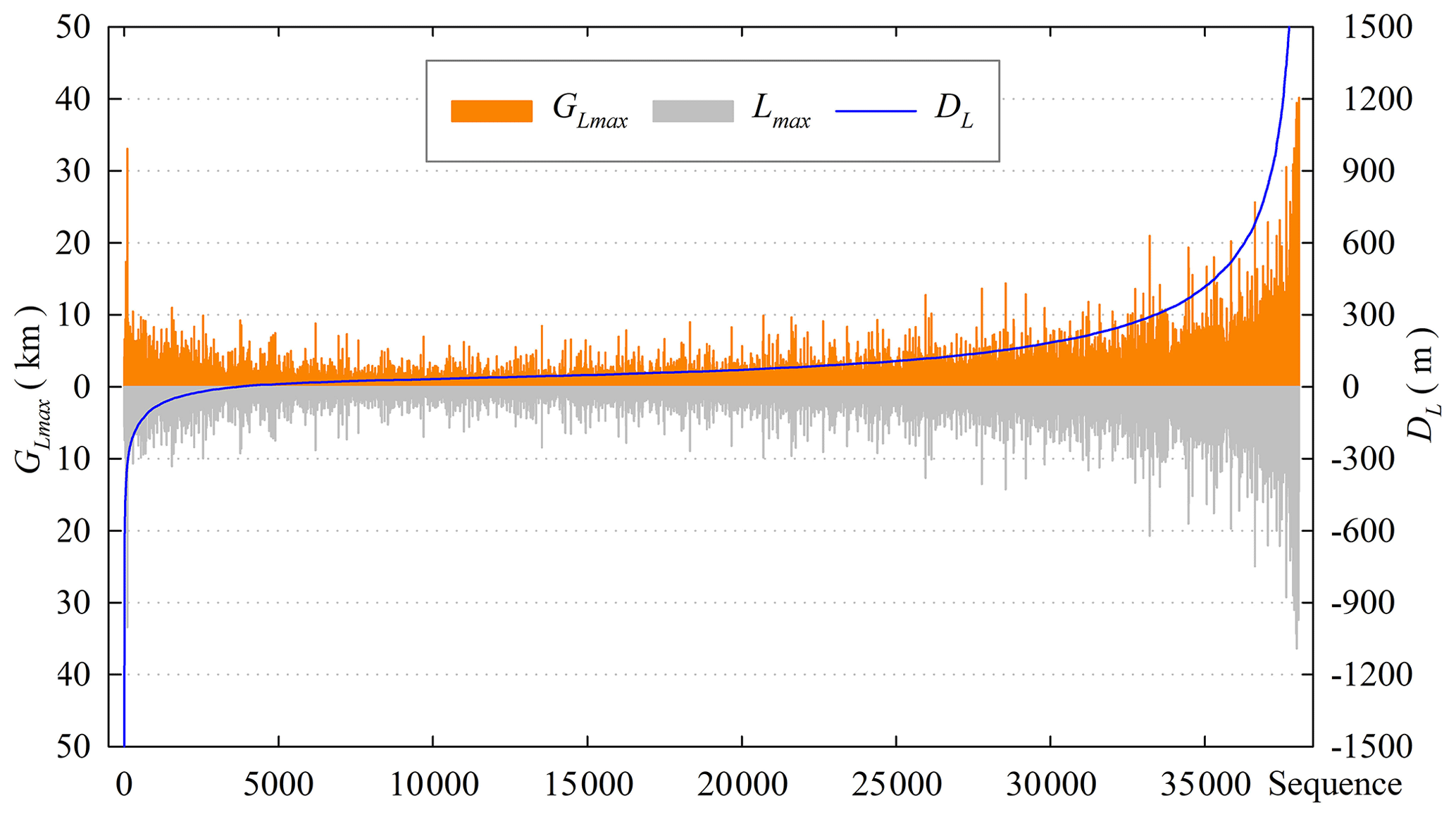
Figure 11The statistical chart of the difference (DL) of the longest glacier length between this dataset (GLmax) and the RGI v6.0 (Lmax).
4.3 Statistics of different samples
According to the standards in Table 3, the selected samples were conducted with visual investigation. The results of nine samples were displayed in Fig. 9. The statistical results showed that the accuracy of verification 2 was the highest (95.25 %), followed by verification 3 (94.76 %) and verification 1 (93 %). The comprehensive accuracy of glacier centerlines was 94.34 %, of which category I and category II accounted for 86.06 % and 8.28 %, respectively. Meanwhile, we summarized the frequency of each type in each sample based on second-level categories. As seen in Fig. 10, the problems of centerlines of small glaciers were mainly caused by the inaccurate selection of division points due to the insufficient accuracy of DEM (code: 22) and incorrect calculation results of some glaciers with little change in slope (code: 33). The problems of centerlines of large glaciers were mainly concentrated in some types coded in 31 and 32, which needed to be repartitioned and recalculated. In addition, a few problems were found in samples: the upper outlines of the glacier were across the ridgeline, a small number of glaciers were not correctly segmented and the altitude in the glaciers' DEM was abnormal. This implied that the reasonable glacier outlines and accurate DEM data were the prerequisite for extracting glacier centerlines and calculating glacier length.
4.4 Comparison to glaciers' maximum length from the RGI v6.0
4.4.1 The statistic of bit order and DL
In the RGI v6.0, 38 053 glaciers in the SCGI were adopted and accounted for 78.35 % of the total glaciers in China, by checking the GLIMS_ID in both glacier datasets. As mentioned above, the field Lmax, the longest glacier length, was contained in the RGI v6.0. In order to further verify the accuracy of glacier length calculated by this method, we calculated the difference (DL) between GLmax and Lmax and then arranged them in ascending order to generate the distribution diagram of sequence DL (Fig. 11). If DL was negative, it meant that the GLmax of glaciers with the corresponding serial number was smaller than Lmax and vice versa. Overall, there was only a small number of glaciers with extremely large at both ends (Fig. 11). After visual inspection, GLmax was more consistent with the actual status of glaciers.
In addition, the average value of positive DL, the average value of negative DL and the number of glaciers in different levels were calculated (Fig. 12). The size of three pixels for the DEM was used as the statistical tolerance, which means glaciers within the tolerance range were regarded as consistent extraction results. Statistically, there were 22 017 glaciers within tolerance, 925 glaciers with negative DL and 15 111 glaciers with positive DL that are greater than the tolerance. In terms of numerical comparison, GLmax obtained by our method was slightly larger than Lmax in RGI v6.0.
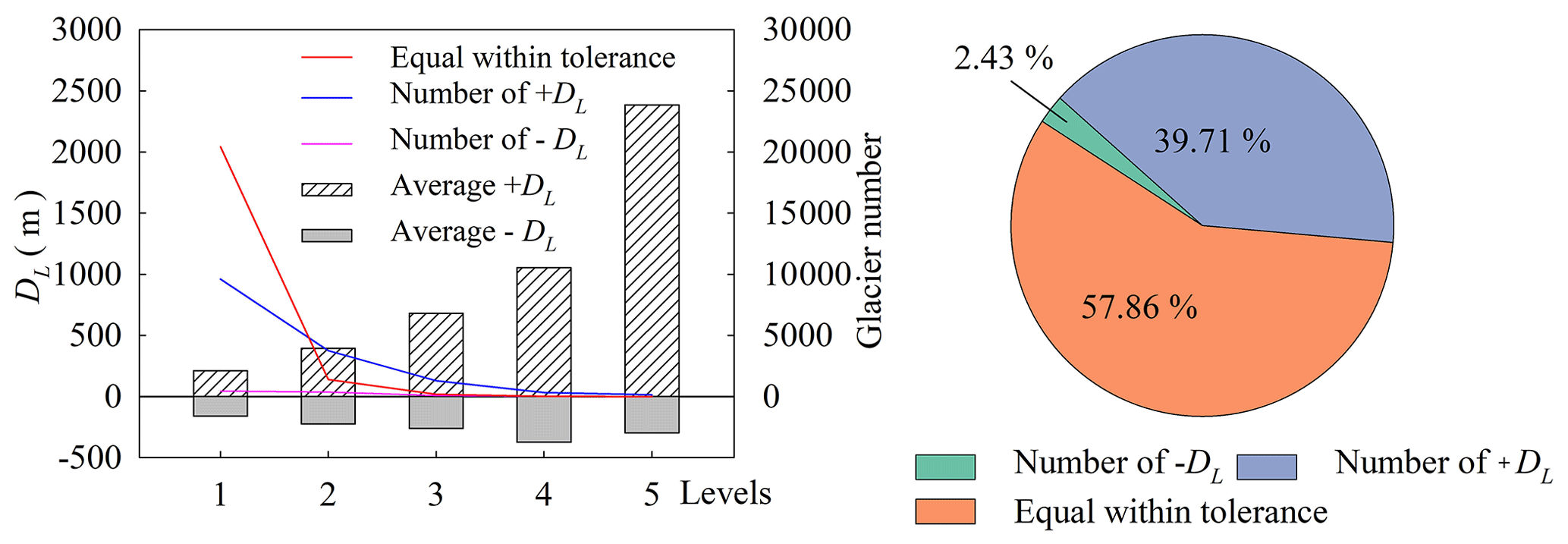
Figure 12The statistical charts of the difference (DL) of the longest length of glaciers by two methods in different glacier sizes.
4.4.2 Analysis of abnormal DL
Combining the designed algorithm with visual inspection, the preliminary analysis showed that the local abnormal DEM, inaccurate glacier outlines and some glacier types (such as ice cap, slope glacier, etc.) were the main causes of abnormal DL (Fig. 13). A slope glacier is a typical multi-origin and multi-exit glacier with almost the same number of local highest points and local lowest points, which often exist in pairs (Fig. 13a). If the local highest point did not match the local lowest point, a value of positive DL would occur (Fig. 13a, blue polyline). Local abnormalities in DEM generally resulted in a shorter GLmax (negative DL), as shown in Fig. 13b. Some key local highest points could not be identified because of the inaccurate outlines, resulting in a large negative DL (Fig. 13c). For a non-single glacier, this algorithm could only identify a lowest point, and all branches of glacier centerlines converge to this point, which would increase the length of most branches and make GLmax too large or even wrong (Fig. 13d).
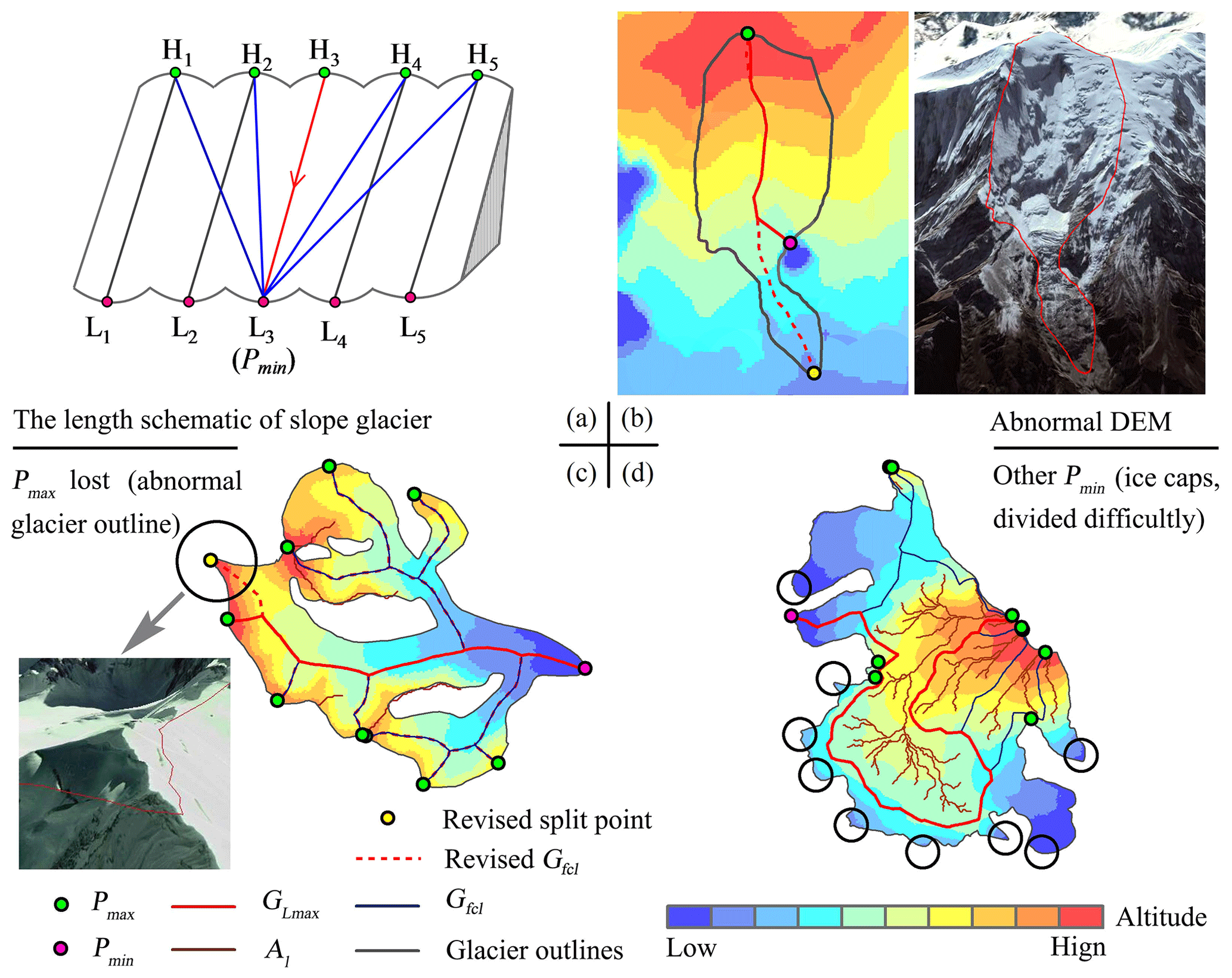
Figure 13The schematic of probable causes for the abnormal of the longest glacier length. In (b), the red dashed line indicates the revised glacier centerline, and the yellow point is the correct lowest point (Pmin). In (c), the red dashed line represents the missing branch, and the yellow point is a local highest point (Pmax) missed by the algorithm. In (d), the black circle indicates some probable exits of the glacier, which needs to be divided into individual glaciers before extracting the centerlines.
The small or abnormal Lmax of some glaciers was also the main reason for abnormal DL. An abnormal example is shown in Fig. 14. The Tugebieliqi Glacier (GLIMS_ID: G080334E42156N) with the maximum is the third largest glacier in China, behind Sugatyanatjilga Glacier and Tuomuer Glacier. Its GLmax was 40.179 km, but its Lmax in the RGI v6.0 was only 11.703 km. The further measurement by Google Earth showed that the west–east length (DW–E) of the glacier was about 27.72 km, which meant that our result was more conformable to reality.
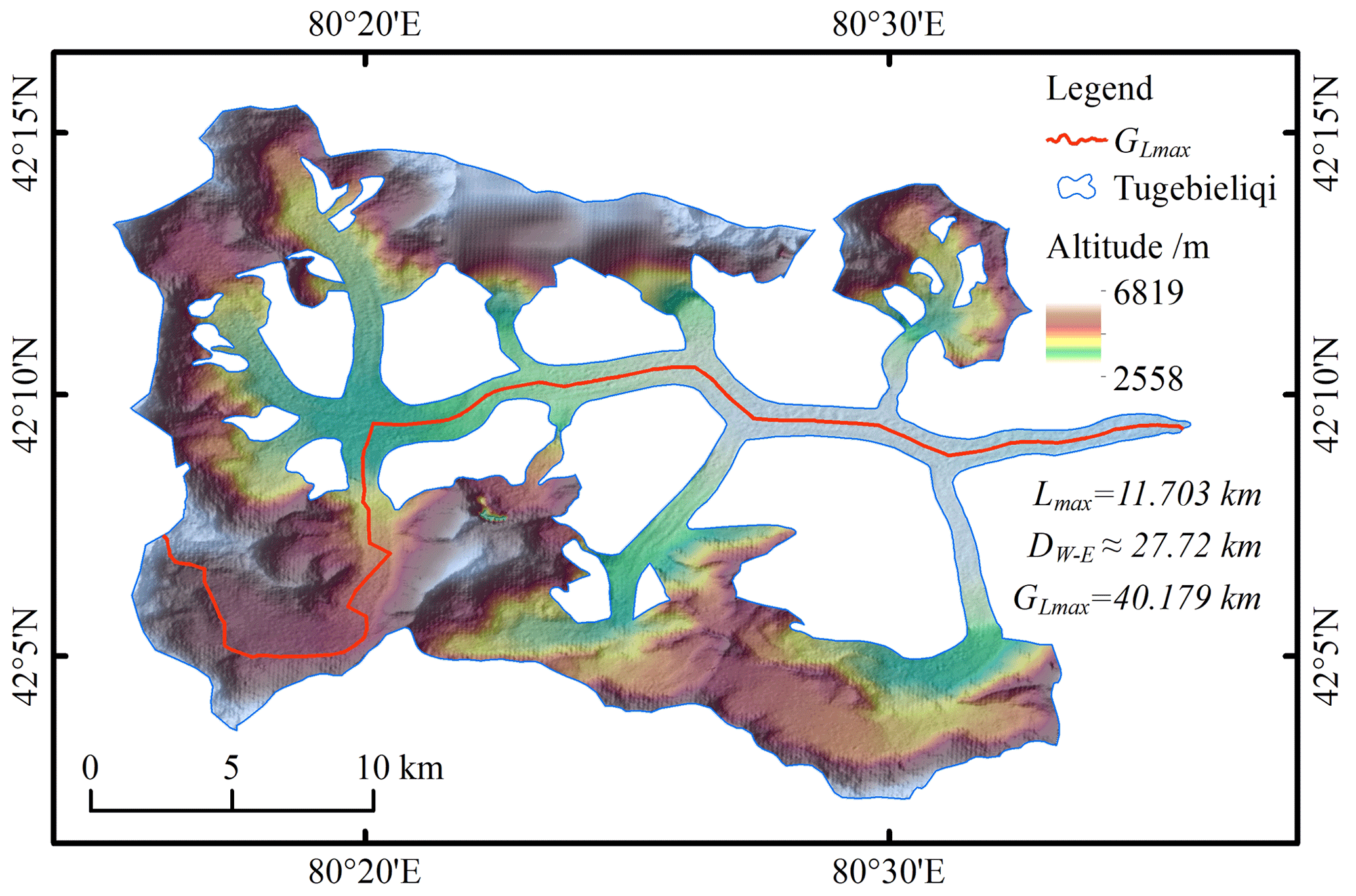
Figure 14The schematic of the longest centerline of Tugebieliqi Glacier (Lmax: the corresponding length of this glacier in the RGI v6.0; DW–E: the distance from west to east of this glacier; GLmax: the length calculated by our method).
5.1 Performance of the algorithm
In the process of extracting centerlines of glaciers in China, all glaciers were equally divided into eight tasks according to the number and considering the running efficiency of the algorithm. Based on the actual extraction results, five glaciers that failed to execute were added as the ninth task. Tasks coded T1–T9 were executed in the working environment of ArcGIS 10.4 software. Except for T7 and T9 using a Lenovo G410 (processors: Intel® Core™ i5-4210M CPU at 2.60 GHz; memory: 4 GB DDR3L 1600 MHz; video card: AMD Radeon R5 M230 2 GB discrete graphics) home laptop, the other seven tasks used seven Dell OptiPlex 7040 (processors: Intel® Core™ i7-6700 CPU at 3.40 GHz; memory: 8 GB DDR4 2633 MHz; video card: AMD Radeon™ R5 340X 2GB integrated graphics) of the tower server with the same configuration. The task distribution and execution results of the tests are given in Table 4.
Table 4The statistics of assigning tasks and results of execution in tests.
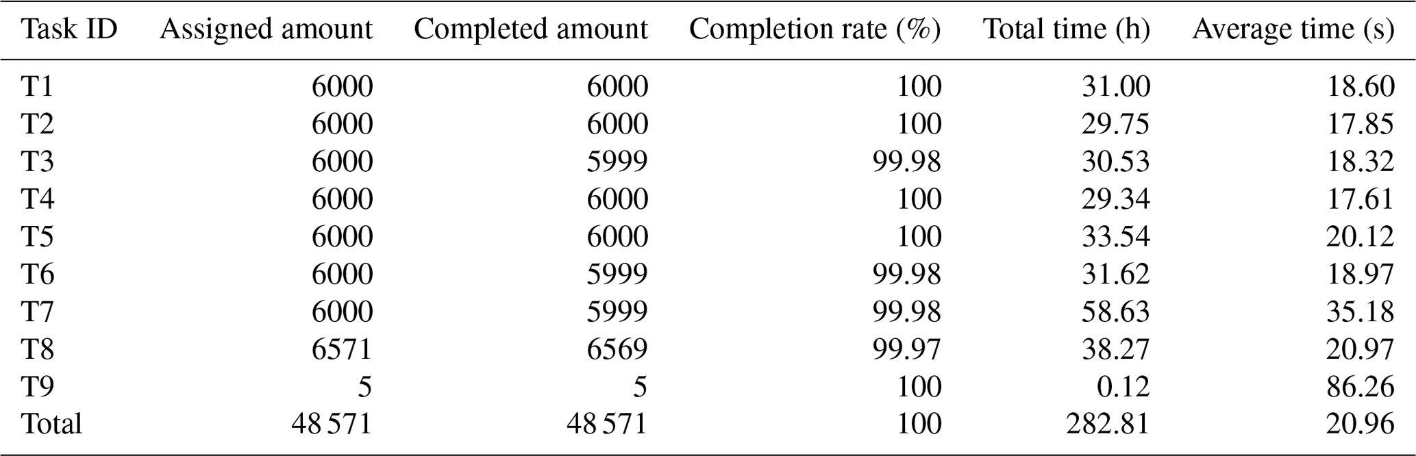
The results of the tests showed that the program took an average of 20.96 s to process an individual glacier, whereas it spent 86.26 s or even longer for some complex glaciers. Among the first eight processing tasks, T4 took the least time. The main reason was that the assigned glaciers in this task were mostly small, and complex glaciers were fewer, except for the higher machine configuration. T7 took the longest time, and the cause was the lower machine configuration. The results of all tasks were merged to obtain the centerline dataset of the SCGI. It contained seven vector files (56 items) and nine logs, which took up about 912 MB in the storage.
5.2 Influence of glacier outline quality and DEM
The extraction method of glacier centerlines belongs to the geometric graphic algorithm and depends on glacier outlines. Natively, compared with the previous studies, our method has similar problems: (i) the delayed shunt and early convergence of the branches and (ii) the centerlines of the same glacier in different periods, which is not geometrically comparable for some glaciers with drastic changes of outlines. The extraction results also showed that the branches of some glacier centerlines did have delayed diversion or early convergence, while the impact on the simulation of the glacier's main flow line was limited. Considering that the results of extracting glacier centerlines change with the changes of glacier outlines, the measurement of the length change of glaciers in different periods will be the focus of our future work. We may further design a new algorithm to automatically supplement, extend, delete or modify the benchmarking glacier centerlines, so as to measure the changes of centerlines and length of glaciers in different periods.
The bare rock region refers to the non-glacial component that is within the outer boundary of the glacier outlines but is not covered by snow or ice. It can be divided into two types: one is the exposed rock protruding on the glacier surface; the other is the cliff generally existing between the upper part of the glacier and the firn basin. The snow or ice on the upper part of the glacier enters the firn basin through the cliffs. And the snow and ice on the cliffs are also important sources of replenishment for firn basin. So the cliffs are theoretically considered to be part of the glacier. However, the cliffs may be similar to the bare rock area during the ablation season, and the cliffs are often accompanied by the presence of image shadows, which will easily cause misjudgments of glacier outlines in interpretation.
Determining the ownership of bare rock regions in Gfl will improve the quality of glacier centerlines. In this study, all bare rock regions were considered to be the first category, and such cases were handled accordingly. The first category was divided into two types: (i) the bare rock area on the upper part of the glacier being equivalent to the ice divide and (ii) the bare rock area near the end of the glacier. The attribution of most bare rock areas in the upper part of the glacier can be determined by the intersection point of Al, Gpl with Gbr. Only a few bare rock areas still exist alone; Eq. (12) was required to determine the segments of the Gfl to which they belong. Some bare rock areas located in the ablation area were allowed to exist alone in the Gfl, and the probability of their existence was extremely low.
The determination of the glacier's ELA is difficult. Some scholars believed that each glacier has its own ELA (Cui and Wang, 2013; Sagredo et al., 2016), but other scholars argued that the ELA of all glaciers in a certain region is the same (Sagredo et al., 2014; Jiang et al., 2018). The measurement of ELA requires continuous and long-term observation data, so it is very difficult to determine the ELA of the glaciers on a large scale. In this study, the ELA used to distinguish between the accumulation area and the ablation area of the glacier was estimated by calculating the median of elevation (Zmed). For some glaciers (such as calving glaciers), the Zmed is above the actual ELA, which has been reasonably explained by scholars (Braithwaite and Raper, 2009). And it was considered that this overestimation is unlikely to affect the automatic calculation of glacier length (Machguth and Huss, 2014).
5.3 Some other factors influencing centerline of glaciers
Automatic extraction of glacier centerlines was basically carried out during the processing of polylines, so the processing algorithm of polylines in the program occupied a considerable part of codes. Among them, several common problems of disconnected polylines are shown in Fig. 15. The following four types are important, which have a great influence on the accuracy and extraction automation of glacier centerlines.
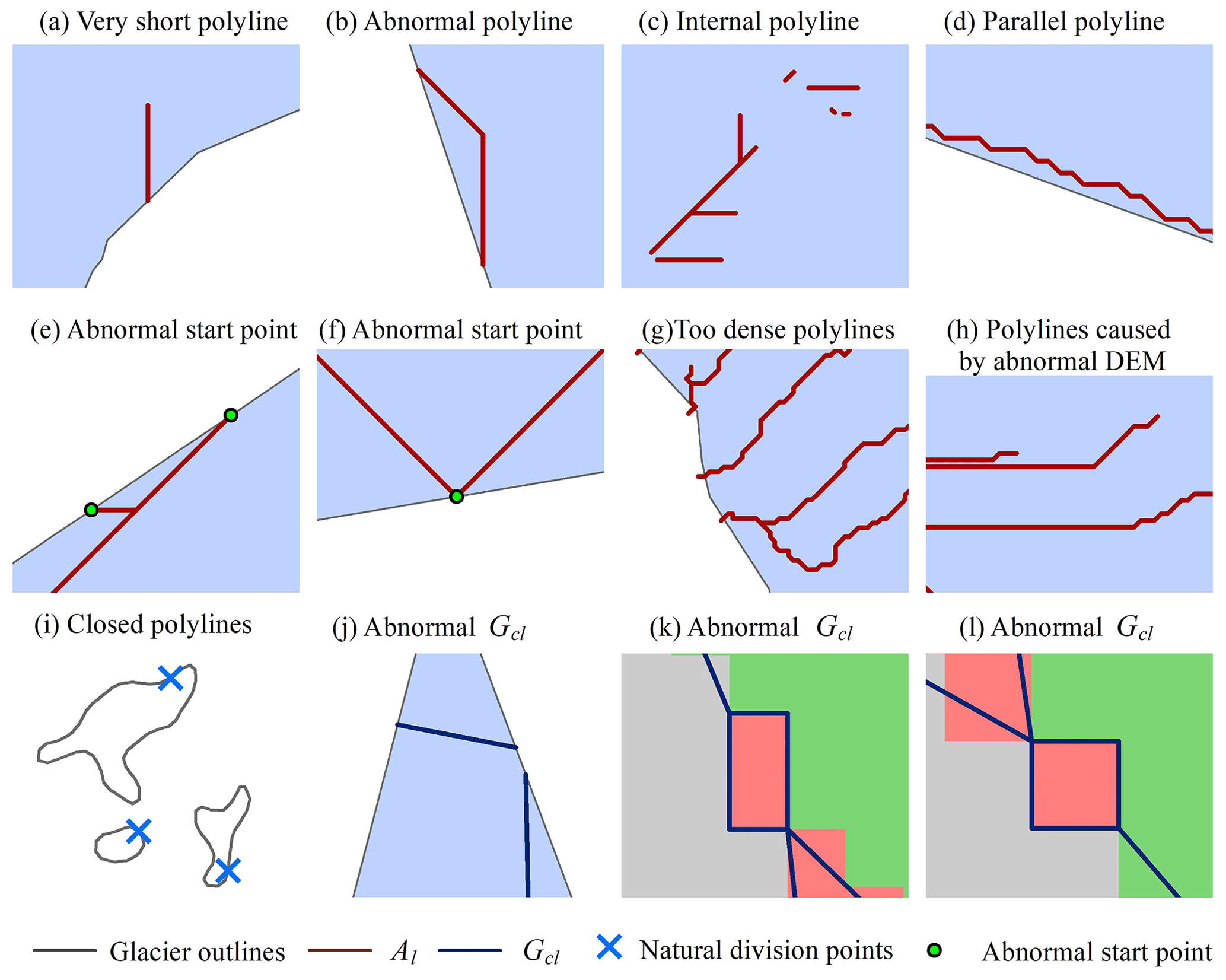
Figure 15The schematic of discontinuous short polylines. Panels (a–h) represent type (i), (i) represents type (ii), (j) represents type (iii) and (k, l) represent type (iv). The background in (a–h) and (j) represents glacier-covered areas. Panel (i) shows several closed polylines, which are not filled with background color. The different background colors in (k, l) represent different areas of the glacier surface after the European allocation.
(i) During the post-processing of the auxiliary lines, due to the inaccuracy of ice divide or the problems of DEM, the ridgelines in the edge of the ice divide of some glaciers start at the Gpl and end up with the Gpl or in parallel along the Gpl, which are unreasonable. In response to this problem, the algorithm set corresponding rules for screening in the processing of auxiliary lines, reducing the impact of such problems as much as possible.
(ii) The visually closed vector polyline is not completely closed. Its start and end are at the same point, which is equal to a natural division point. Unless the natural division point of Gpl completely coincides with a certain division point, the number of polyline records in the Gpl after division will be one more than we expected. Therefore, it is necessary to identify the natural division point during processing and merge the two disconnected polyline records.
(iii) The algorithm of Euclidean allocation is accomplished based on raster operation, which is equivalent to the equidistant scatter operation with the interval of P8 on the glacier surface. For some glaciers with horizontal or vertical distribution of the Gpl, the extraction will continue after the centerlines overlap with the Gpl. We only need to design the corresponding functions to detect and delete this redundancy of the disconnected polylines.
(iv) In the process of calling the module of Euclidean allocation to generate the centerlines, there is a slight probability that pixels with strictly equal distances will appear. The central axis will generate a regular rectangle based on the raster pixel corresponding to the central point, which will affect the calculation of the GLmax. In the algorithm, a function to identify and deal with such problems was added after the Euclidean allocation, and then the polylines on one side of the diagonal of a rectangle were randomly retained.
An automatic method for extracting glacier centerlines based on Euclidean allocation in two-dimensional space was designed and implemented in this study. It only needs the glacier outlines and the corresponding DEM to automatically generate the vector data of glacier centerlines and provides different properties including the longest length, the average length, the length in the ablation region and the length in the accumulation region of the glacier. The standardized and automatic extraction of glacier centerlines requires no manual intervention. Meanwhile, we used the SCGI as the test data to run the program and verify its efficiency. The success rate of extracting glacier centerlines was very close to 100 %, and the comprehensive extraction accuracy reached 94.34 %, which reflected the robustness and simplicity of this method.
The automatic extraction algorithm proposed has three advantages: (i) introducing the auxiliary reference lines which ensure the validity of the upper glacier centerlines, (ii) success in automatically obtaining the longest centerline of each glacier and the branches of glacier centerlines and (iii) providing more information of glacier lengths than other methods proposed by some scholars. Compared with the longest length of each glacier in the RGI v6.0, the length of the corresponding glacier calculated by our algorithm is in better agreement with the actual length of the glacier. We also identified the possible causes affecting the accuracy of glacier centerlines. In the future, we will focus on improving the time efficiency of the algorithm, providing the updated datasets of glacier centerlines with higher quality and identifying the abnormal glacier phenology such as rapid glacier surge.
The paper uses numerous abbreviations. Explanations of the main acronyms are listed in Table A1.
| At | The given area of an equilateral triangle |
| Ag | The polygon's area of the glacier's outer boundary |
| Al | The final auxiliary line |
| Ar | The ridgelines of the glacier surface |
| Gbr | The bare rock in the glacier |
| Gfcl | The final glacier centerline |
| Gfl | The feature lines of the glacier surface |
| Gcl | Glacier centerline |
| GLabl | The length in the ablation region of the glacier |
| GLacc | The length in the accumulation region of the glacier |
| GLmax | The longest length of the glacier |
| GLmean | The average length of the glacier |
| Gpl | The polyline of the outer boundary of the glacier |
| Gpo | The polygon of the outer boundary of the glacier |
| Lmax | The longest glacier length of RGI v6.0 |
| DL | The difference between GLmax and Lmax |
| Pt | The given perimeter of an equilateral triangle |
| Pg | The perimeter of the glacier's outer boundary |
| Pmax | The highest local point of glacier outline |
| Pmin | The lowest point of glacier outline |
| RGI | The Randolph Glacier Inventory |
| SCGI | The Second Chinese Glacier Inventory |
| Zmed | The median elevation of the glacier |
The code used to support the findings of this study are available in the Supplement.
The datasets including the SCGI, RGI v6.0 and SRTM1 DEM v3.0 used in this study are freely available. The database of glacier centerlines in the SCGI produced in this study are available from the corresponding author upon request.
The Supplement consists of three parts. They are (i) automatic extraction software of glacier centerlines, (ii) software instructions and (iii) some test results. The supplement related to this article is available online at: https://doi.org/10.5194/tc-15-1955-2021-supplement.
XY designed this algorithm of extracting glacier centerlines and edited the manuscript. DZ implemented the program and wrote the first draft of the manuscript. HD tested the program and checked the quality of glacier centerlines. SL, WG, MS and DL reviewed and edited the manuscript.
The authors declare that they have no conflict of interest.
We thank editors and the two reviewers for their valuable comments that improved the manuscript. Dahong Zhang thanks his current supervisor, Professor Shiqiang Zhang of Northwest University in Xi'an, China, for valuable ideas and suggestions.
This research has been supported by the National Natural Science Foundation of China (grant nos. 41861013, 42071089 and 41801052), the Open Research Fund of the National Earth Observation Data Center (grant no. NODAOP2020007) and the Open Research Fund of the National Cryosphere Desert Data Center (grant no. 20D02).
This paper was edited by Alexander Robinson and reviewed by two anonymous referees.
Braithwaite, R. J. and Raper, S. C. B.: Estimating equilibrium-line altitude (ELA) from glacier inventory data, Ann. Glaciol., 50, 127–132, https://doi.org/10.3189/172756410790595930, 2009.
Cui, H. and Wang, J.: The methods for estimating the equilibrium line altitudes of a glacier, Journal of Glaciology and Geocryology, 35, 345–354, 2013.
Farr, T. G., Rosen, P. A., Caro, E., Crippen, R., Duren, R., Hensley, S., Kobrick, M., Paller, M., Rodriguez, E., Roth, L., Seal, D., Shaffer, S., Shimada, J., Umland, J., Werner, M., Oskin, M., Burbank, D., and Alsdorf, D.: The Shuttle Radar Topography Mission, Rev. Geophys., 45, 1–33, https://doi.org/10.1029/2005rg000183, 2007.
Gao, Y. P., Yao, X. J., Liu, S. Y., Qi, M. M., Gong, P., An, L. N., Li, X. F., and Duan, H. Y.: Methods and future trend of ice volume calculation of glacier, Arid Land Geography, 41, 1204–1213, 2018.
Gao, Y. P., Yao, X. J., Liu, S. Y., Qi, M. M., Duan, H. Y., Liu, J., and Zhang, D. H.: Remote sensing monitoring of advancing glaciers in the Bukatage Mountains from 1973 to 2018, Journal of Natural Resources, 34, 1666–1681, https://doi.org/10.31497/zrzyxb.20190808, 2019.
Guo, W., Liu, S., Xu, J., Wu, L., Shangguan, D., Yao, X., Wei, J., Bao, W., Yu, P., Liu, Q., and Jiang, Z.: The second Chinese glacier inventory: data, methods and results, J. Glaciol., 61, 357-372, https://doi.org/10.3189/2015JoG14J209, 2017.
Heid, T. and Kääb, A.: Repeat optical satellite images reveal widespread and long term decrease in land-terminating glacier speeds, The Cryosphere, 6, 467–478, https://doi.org/10.5194/tc-6-467-2012, 2012.
Herla, F., Roe, G. H., and Marzeion, B.: Ensemble statistics of a geometric glacier length model, Ann. Glaciol., 58, 130–135, https://doi.org/10.1017/aog.2017.15, 2017.
Ji, Q., Yang, T.-B., He, Y., Qin, Y., Dong, J., and Hu, F.-S.: A simple method to extract glacier length based on Digital Elevation Model and glacier boundaries for simple basin type glacier, J. Mt. Sci., 14, 1776–1790, https://doi.org/10.1007/s11629-016-4243-5, 2017.
Jiang, D. B., Liu, Y. Y., and Lang, X. M.: A multi-model analysis of glacier equilibrium line altitudes in western China during the Last Glacial Maximum, Science China Earth Sciences, 49, 1231–1245, https://doi.org/10.1360/n072018-00058, 2018.
Kienholz, C., Rich, J. L., Arendt, A. A., and Hock, R.: A new method for deriving glacier centerlines applied to glaciers in Alaska and northwest Canada, The Cryosphere, 8, 503–519, https://doi.org/10.5194/tc-8-503-2014, 2014.
Le Bris, R. and Paul, F.: An automatic method to create flow lines for determination of glacier length: A pilot study with Alaskan glaciers, Comput. Geosci., 52, 234–245, https://doi.org/10.1016/j.cageo.2012.10.014, 2013.
Leclercq, P. W. and Oerlemans, J.: Global and hemispheric temperature reconstruction from glacier length fluctuations, Clim. Dynam., 38, 1065–1079, https://doi.org/10.1007/s00382-011-1145-7, 2012.
Leclercq, P. W., Pitte, P., Giesen, R. H., Masiokas, M. H., and Oerlemans, J.: Modelling and climatic interpretation of the length fluctuations of Glaciar Frías (north Patagonian Andes, Argentina) 1639–2009 AD, Clim. Past, 8, 1385–1402, https://doi.org/10.5194/cp-8-1385-2012, 2012a.
Leclercq, P. W., Weidick, A., Paul, F., Bolch, T., Citterio, M., and Oerlemans, J.: Brief communication “Historical glacier length changes in West Greenland”, The Cryosphere, 6, 1339–1343, https://doi.org/10.5194/tc-6-1339-2012, 2012b.
Leclercq, P. W., Oerlemans, J., Basagic, H. J., Bushueva, I., Cook, A. J., and Le Bris, R.: A data set of worldwide glacier length fluctuations, The Cryosphere, 8, 659–672, https://doi.org/10.5194/tc-8-659-2014, 2014.
Li, H., Ng, F., Li, Z., Qin, D., and Cheng, G.: An extended “perfect-plasticity” method for estimating ice thickness along the flow line of mountain glaciers, J. Geophys. Res.-Earth, 117, 1020–1030, https://doi.org/10.1029/2011jf002104, 2012.
Linsbauer, A., Paul, F., and Haeberli, W.: Modeling glacier thickness distribution and bed topography over entire mountain ranges with GlabTop: Application of a fast and robust approach, J. Geophys. Res.-Earth, 117, 3007–3024, https://doi.org/10.1029/2011jf002313, 2012.
Liu, S. Y., Yao, X. J., Guo, W. Q., Xu, J. L., Shang Guan, D. H., Wei, J. F., Bao, W. J., and Wu, L. Z.: The contemporary glaciers in China based on the Second Chinese Glacier Inventory, Acta Geographica Sinica, 70, 3–16, https://doi.org/10.11821/dlxb201501001, 2015.
Machguth, H. and Huss, M.: The length of the world's glaciers – a new approach for the global calculation of center lines, The Cryosphere, 8, 1741–1755, https://doi.org/10.5194/tc-8-1741-2014, 2014.
McNabb, R. W., Hock, R., O'Neel, S., Rasmussen, L. A., Ahn, Y., Braun, M., Conway, H., Herreid, S., Joughin, I., Pfeffer, W. T., Smith, B. E., and Truffer, M.: Using surface velocities to calculate ice thickness and bed topography: a case study at Columbia Glacier, Alaska, USA, J. Glaciol., 58, 1151–1164, https://doi.org/10.3189/2012JoG11J249, 2017.
Melkonian, A. K., Willis, M. J., and Pritchard, M. E.: Satellite-derived volume loss rates and glacier speeds for the Juneau Icefield, Alaska, J. Glaciol., 60, 743–760, https://doi.org/10.3189/2014JoG13J181, 2017.
Muhuri, A., Natsuaki, R., Bhattacharya, A., and Hirose, A.: Glacier Surface Velocity Estimation Using Stokes Vector Correlation, Synthetic Aperture Radar, Singapore, 2015, ISBN: 9781467372961, 606–609, 2015.
Nuth, C., Kohler, J., König, M., von Deschwanden, A., Hagen, J. O., Kääb, A., Moholdt, G., and Pettersson, R.: Decadal changes from a multi-temporal glacier inventory of Svalbard, The Cryosphere, 7, 1603–1621, https://doi.org/10.5194/tc-7-1603-2013, 2013.
Oerlemans, J.: A flowline model for Nigardsbreen, Norway: projection of future glacier length based on dynamic calibration with the historic record, Ann. Glaciol., 24, 382–389, https://doi.org/10.1017/S0260305500012489 1997.
Paul, F., Barry, R. G., Cogley, J. G., Frey, H., Haeberli, W., Ohmura, A., Ommanney, C. S. L., Raup, B., Rivera, A., and Zemp, M.: Recommendations for the compilation of glacier inventory data from digital sources, Ann. Glaciol., 50, 119–126, https://doi.org/10.3189/172756410790595778, 2009.
Sagredo, E. A., Rupper, S., and Lowell, T. V.: Sensitivities of the equilibrium line altitude to temperature and precipitation changes along the Andes, Quaternary Res., 81, 355–366, https://doi.org/10.1016/j.yqres.2014.01.008, 2014.
Sagredo, E. A., Lowell, T. V., Kelly, M. A., Rupper, S., Aravena, J. C., Ward, D. J., and Malone, A. G. O.: Equilibrium line altitudes along the Andes during the Last millennium: Paleoclimatic implications, Holocene, 27, 1019–1033, https://doi.org/10.1177/0959683616678458, 2016.
Schiefer, E., Menounos, B., and Wheate, R.: An inventory and morphometric analysis of British Columbia glaciers, Canada, J. Glaciol., 54, 551–560, https://doi.org/10.3189/002214308785836995 2008.
Sugiyama, S., Bauder, A., Zahno, C., and Funk, M.: Evolution of Rhonegletscher, Switzerland, over the past 125 years and in the future: application of an improved flowline model, Ann. Glaciol., 46, 268–274, https://doi.org/10.3189/172756407782871143 2007.
Winsvold, S. H., Andreassen, L. M., and Kienholz, C.: Glacier area and length changes in Norway from repeat inventories, The Cryosphere, 8, 1885–1903, https://doi.org/10.5194/tc-8-1885-2014, 2014.
Yang, B. Y., Zhang, L. X., Gao, Y., Xiang, Y., Mou, N. X., and Suo, L. D. B.: An integrated method of glacier length extraction based on Gaofen satellite data, Journal of Glaciology and Geocryology, 38, 1615–1623, 2016.
Yao, X. J., Liu, S. Y., Zhu, Y., Gong, P., An, L. N., and Li, X. F.: Design and implementation of an automatic method for deriving glacier centerlines based on GIS, Journal of Glaciology and Geocryology, 37, 1563–1570, 2015.
Zhang, W. and Han, H. D.: A review of the ice volume estimation of mountain glaciers, Journal of Glaciology and Geocryology, 38, 1630–1643, 2016.
- Abstract
- Introduction
- Input data and test region
- Principles and algorithm of glacier centerline extraction
- Accuracy evaluation and the results
- Discussion
- Conclusions
- Appendix A: The list of main acronyms in this study
- Code availability
- Data availability
- Author contributions
- Competing interests
- Acknowledgements
- Financial support
- Review statement
- References
- Supplement