Impact of updated radiative transfer scheme in snow and ice in RACMO2.3p3 on the surface mass and energy budget of the Greenland ice sheet

Radiative transfer in snow and ice is often not modeled explicitly in regional climate models. In this study, we evaluate a new englacial radiative transfer scheme and assess the surface mass and energy budget for the Greenland ice sheet in the latest version of the regional climate model RACMO2, version 2.3p3. We also evaluate the modeled (sub)surface temperature and melt, as radiation penetration now enables internal heating. The results are compared to the previous model version and are evaluated against stake measurements and automatic weather station data of the K-transect and PROMICE projects. In addition, subsurface snow temperature profiles are compared at the K-transect, Summit, and southeast Greenland. The surface mass balance is in good agreement with observations, with a mean bias of −31 mm w.e. yr⁻¹ (−2.67 %), and only changes considerably with respect to the previous RACMO2 version around the ice margins and near the percolation zone. Melt and refreezing, on the other hand, are changed more substantially in various regions due to the changed albedo representation, subsurface energy absorption, and meltwater percolation. Internal heating leads to higher snow temperatures in summer, in agreement with observations, and introduces a shallow layer of subsurface melt. Hence, this study shows the consequences and necessity of radiative transfer in snow and ice for regional climate modeling of the Greenland ice sheet.

1 Introduction

The Greenland ice sheet (GrIS) has been losing mass at an accelerating pace in the last decade (Box and Colgan, 2013; Kjeldsen et al., 2015; Bevis et al., 2019; Shepherd et al., 2020). Both surface runoff and solid ice discharge have increased, enhancing mass loss (Bigg et al., 2014). The relative contribution of surface processes with respect to ice discharge, however, has recently increased considerably (Enderlin et al., 2014; Kjeldsen et al., 2015; Mouginot et al., 2019), augmenting the need to accurately model the surface mass balance (SMB) in regional and global climate models.

The SMB, which is the difference between precipitation and ablation, i.e., runoff, sublimation, and drifting snow erosion, is highly variable in space and time. Snow and ice melt leading to extensive runoff typically dominates the SMB around the margins of the GrIS, leading to mass loss of up to 3 m water equivalent (w.e.) yr⁻¹, while snowfall dominates in the interior (Van den Broeke et al., 2016). In the interior, melt events do not necessarily lead to runoff, as a significant fraction of all meltwater refreezes locally (Steger et al., 2017). The length and spatial extent of melt events vary from year to year, but record-breaking melt events like during the summer of 2012 and 2019 can bring melt to almost the entire ice sheet (Nghiem et al., 2012; Bennartz et al., 2013; Tedesco et al., 2013; Tedesco and Fettweis, 2020), enhancing snow metamorphism and lowering the albedo, i.e., the fraction of incoming shortwave radiation that is reflected. As similar melt events are expected to become more common in a warmer climate (IPCC, 2013; Shepherd et al., 2020), it is therefore important to adequately resolve the individual SMB components. In situ observations, however, lack the required spatial coverage and temporal sampling to fully capture these events, while satellites cannot adequately quantify melt rates, and thus the use of climate models is required (Rae et al., 2012; Goelzer et al., 2013; Leeson et al., 2018; Alexander et al., 2019).

Regional climate models (RCMs) are able to explicitly resolve the GrIS SMB components and other atmospheric and surface processes and are characterized by a high temporal (subhourly) and spatial resolution (up to 5 km) (Fettweis et al., 2017; Langen et al., 2017; Powers et al., 2017; Niwano et al., 2018; Noël et al., 2018b). RCMs are known to perform well for most of the ice sheet, but they struggle to resolve topographically inhomogeneous regions (Leeson et al., 2018). Statistically downscaling the SMB components to an even higher resolution of up to 1 km (Noël et al., 2019) solves many such issues. Still, the rough topography typically found close to the ice margin is often not modeled correctly and can lead to incorrect precipitation patterns, which illustrates the need to further improve SMB-related parameterizations (Van de Berg et al., 2020).

Surface melt rate is determined by the surface energy budget (SEB), i.e., the sum of radiative, turbulent, and subsurface heat fluxes. A considerable part of incoming shortwave radiation, however, penetrates through the surface, heating snow and ice layers below (Kuipers Munneke et al., 2009; Warren, 2019; He and Flanner, 2020). This is especially important if ice rather than snow is at or close to the surface. Radiation scattering is limited in these large-grained ice layers, and shortwave radiation is therefore also absorbed below the surface, acting as a heat source. As internal heat is not as effectively dissipated as at the surface, subsurface energy absorption can lead to subsurface melting if the surface is close to or at the melting point.

Parameterizations of radiative fluxes can still be improved in RCMs. The Modèle Atmosphérique Régional (MAR), for example, uses the Surface Vegetation Atmosphere Transfer scheme SISVAT (Gallée et al., 1991; De Ridder and Gallée, 1998; Fettweis, 2007; Fettweis et al., 2017). SISVAT does not contain a proper radiative transfer scheme in snow or ice; the albedo is therefore parameterized by using various tuning parameters. Internal heating by shortwave radiation is also not calculated and is therefore not included in the heat balance of a layer. Similarly, the RCM HIRHAM5 (Lucas-Picher et al., 2012), which uses the physics of the ECHAM5 model (Roeckner et al., 2003), does not consider radiative transfer in snow and ice, and the snow albedo is calculated simply as a linear function with the surface temperature. The RCM that we use in this study, the polar (p) version of the Regional Atmospheric Climate Model (RACMO2), also does not include radiation penetration.

RACMO2 has been used extensively to model large-scale, ice-sheet-wide developments of the Greenland (Noël et al., 2018b, 2019) and Antarctic ice sheets (Van de Berg and Medley, 2016; Van Wessem et al., 2018) but also for glaciated areas on a smaller scale, like the glaciers and ice caps of the Canadian Arctic (Noël et al., 2018a). Furthermore, RACMO2 has been used to investigate physical processes like the snowmelt–albedo feedback (Jakobs et al., 2019) and föhn winds (Wiesenekker et al., 2018). Recent improvements in snow albedo parameterizations and radiation transfer schemes now allow the implementation of a radiation penetration module in RACMO2 (Van Dalum et al., 2019). The new version RACMO2.3p3, henceforth Rp3, incorporates a new snow and ice albedo and radiative transfer scheme, which includes internal heating by radiation penetration, and updates to the firn module (Van Dalum et al., 2020a).

In this paper we assess the impact of the improved radiative transfer scheme in snow and ice on the modeled SMB and SEB for the GrIS in Rp3. Section 2 discusses the model and initialization; expands on the concepts of SMB, SEB, and internal energy absorption; and discusses the in situ data sets in more detail. In Sect. 3, internal energy absorption due to radiation penetration is assessed. In Sect. 4, sensitivity experiments further highlight the impact of internal heating on the subsurface temperature. Results are compared with observations and compared to the previous RACMO2 version, 2.3p2 (Rp2) (Noël et al., 2018b) and to a Rp3 model version without internal energy absorption (Rp3 WIE). In Sect. 5, results are analyzed by evaluating the SEB compared to observations and by comparing modeled SEB of Rp3 with Rp2. Similar to Sect. 5, Sect. 6 focuses on the SMB and its components. We also compare the SMB of Rp3 with Rp3 WIE. Finally, Sect. 7 summarizes the results, and conclusions are drawn.

2 Methods and data

2.1 Regional climate model

The Regional Atmospheric Climate Model (RACMO2), developed at the Royal Netherlands Meteorological Institute (KNMI), couples the surface and atmospheric processes of the European Centre for Medium-Range Weather Forecasts (ECMWF) Integrated Forecast System (IFS), cycle 33r1 (ECMWF, 2009), with the atmospheric dynamics of the High Resolution Limited Area Model, version 5.0.3 (HIRLAM, Undén et al., 2002). The polar (p) version of RACMO2, which is developed at the Institute for Marine and Atmospheric Research Utrecht (IMAU), is adjusted for glaciated areas by introducing a dedicated glaciated tile that includes snow and ice processes and more complete ice–atmosphere interaction (Noël et al., 2015). Two major components have been updated in the new version Rp3 compared to the previous version Rp2: the multilayer firn module and the snow and ice albedo parameterization, which makes use of a radiative transfer scheme.

2.1.1 Multilayer firn module

Four modifications have been applied to the multilayer firn module, which we briefly address here and are discussed in more detail in Van Dalum et al. (2020a). Firstly, Rp2 uses a prognostic fresh snow layer, which is effectively a sublayer of the uppermost snow layers. This sublayer is removed, and the uppermost snow layers are now allowed to be as thin as a few millimeters. Secondly, if merging is necessary, a snow layer now merges with its most similar adjacent layer instead of the next layer. Numerical diffusion is prevented by redistributing mass if a thin layer merges with a thick layer. Layers formed by local accumulation are not allowed to merge with glacial ice. Furthermore, the effective vertical resolution has increased, with typically 50 to 60 active snow layers, up to a maximum of 100. Model output, however, is only available for the first 20 layers. Thirdly, internal melt will thin a subsurface snow layer if the density is lower than 700 kg m⁻³. Pore space is created for ice layers with a density of more than 830 kg m⁻³. A combination of both occurs for firn with intermediate densities. Melting of the upper layer always leads to thinning. Finally, the initialized ice density is changed from 910 in Rp2 to 917 kg m⁻³ in Rp3.

2.1.2 Snow albedo and radiative transfer

The plane-parallel broadband snow albedo scheme based on Gardner and Sharp (2010) is replaced by the Two-streAm Radiative TransfEr in Snow Model (TARTES; Libois et al., 2013), which is coupled to RACMO2 with the Spectral-to-NarrOWBand ALbedo (SNOWBAL) module version 1.2 (Van Dalum et al., 2019). The broadband albedo parameterization of Gardner and Sharp (2010) is based on tuning parameters and lookup tables and parameterizes the albedo impact of SZA, wavelength of irradiance, grain radius, cloud cover, and impurities. Only the upper snow layer is considered for its calculations, with the second layer as a semi-infinite background layer. As the upper snow layers in RACMO2 are often only millimeters thick, there is virtually no radiation penetration in Rp2.

The albedo scheme of Rp3 is fundamentally different, as TARTES uses the asymptotic radiative transfer theory (Kokhanovsky, 2004; He and Flanner, 2020) and the radiative transfer equation (Jiménez-Aquino and Varela, 2005) to calculate a spectral albedo and subsurface energy absorption by using the geometric-optics method. Spectral radiative transfer in TARTES depends on snow layer density, impurity concentration, grain radius, and grain shape. Here, grains are assumed to be spherically shaped, and prognostic estimates are provided for the other variables by the multilayer firn model. SNOWBAL has been developed to couple the output of TARTES with the 14 contiguous shortwave spectral bands of the IFS physics scheme embedded in RACMO2, taking into account sub-band variations in both the albedo and the irradiance. SNOWBAL selects a predefined representative wavelength for given atmospheric conditions suitable for TARTES to use, such that a narrowband albedo and subsurface energy flux can be accurately represented by one spectral evaluation of TARTES (Van Dalum et al., 2019). The representative wavelength depends on the SZA and vertically integrated water vapor for clear-sky conditions and ice and liquid water path for cloudy conditions. Bands 13 and 14, covering 3077–3845 and 3846–12 500 nm, respectively, are excluded from calculations, as the albedo for these bands can be safely assumed to be zero (Gardner and Sharp, 2010), and all energy contributes to the SEB.

2.1.3 Ice albedo

Additionally, a new bare-ice albedo parameterization using both TARTES and SNOWBAL has been developed. In Rp2, the bare-ice albedo is prescribed by the lowest 5 % of the 16 d diffuse albedo product of 1 km MODIS data (MCD43A3v5; Schaaf and Wang, 2015), resampled to the RACMO2 grid and limited between 0.3 for dark ice and 0.55 for perennial snow (Noël et al., 2018b). In Rp3, we replace these predefined bare-ice albedos by using TARTES and SNOWBAL for each spectral band, allowing for varying bare-ice albedo and estimates of subsurface heating. TARTES, however, is not suitable to be applied directly to ice, as it is not based on Mie-scattering theory, and some approximations have to be made.

Firstly, we determine the specific surface area (SSA) of a semi-infinite ice layer such that TARTES and SNOWBAL calculate a broadband albedo of 0.6, which represents the broadband albedo of clean blue ice (Reijmer et al., 2001; Dadic et al., 2013) for clear-sky conditions and a reference SZA of 60^∘. For this, we find an SSA of 0.788 m² kg⁻¹ (4.152 mm grain size). Then, using this SSA and SZA, a broadband albedo can be determined for a range of impurities. With this impurity range, the MCD43A3v5 MODIS albedo can be converted into an impurity concentration for each model grid point. Each time a layer is identified as bare ice, TARTES and SNOWBAL use the prescribed SSA and impurity field to do its calculations. For subsurface glacial ice layers, we use this procedure as well. Superimposed ice is treated differently than glacial ice, as it is formed by refreezing of meltwater in snow layers and has a granular structure (Granskog et al., 2006). In Rp3, superimposed ice is therefore treated as a snow layer, with a minimum grain radius of 0.720 mm for a layer density of 750 kg m⁻³, and the grain radius increases linearly to the bare-ice value of 4.152 mm for a density of 917 kg m⁻³. A more detailed model description, evaluation, and discussion of the snow and ice albedo product can be found in Van Dalum et al. (2020a).

2.2 Surface mass balance and surface energy budget

The surface energy budget (SEB) of RACMO2, with fluxes toward the surface defined as positive, is defined as

$$\begin{array}{}\text{(1)}& M={\mathrm{LW}}_{\mathrm{d}}+{\mathrm{LW}}_{\mathrm{u}}+{\mathrm{SW}}_{\mathrm{d}}+{\mathrm{SW}}_{\mathrm{u}}+\mathrm{SHF}+\mathrm{LHF}+G_{\mathrm{s}},\end{array}$$

with M the surface melt flux (M=0 when surface temperature T_s<273.15 K); LW_d, LW_u, SW_d, and SW_u the downward and upward longwave radiative fluxes and downward and upward shortwave radiative fluxes, respectively; SHF and LHF the sensible and latent heat fluxes; and G_s the subsurface conductive heat flux, all in W m⁻². Meltwater is allowed to percolate into deeper layers using the tipping-bucket method; i.e., water fills a layer until irreducible water saturation is reached (Coléou and Lesaffre, 1998). Excess water moves to the next unsaturated layer, where it can refreeze, be retained, or run off. There is no lateral flow between grid points. The subsurface conductive heat flux G_s is the energy flux between the skin layer, i.e., the contact layer between the atmosphere and the surface, and the uppermost layer of the firn column. Between all model layers, G_s is also derived and used for the subsurface temperature evolution, but this flux is not stored.

Here, we adopt the following definition of the surface mass balance (SMB), in mm w.e. yr⁻¹:

$$\begin{array}{}\text{(2)}& \mathrm{SMB}=\mathrm{SN}+\mathrm{RA}-\mathrm{ER}-\mathrm{SU}-\mathrm{RU},\end{array}$$

with SN as snowfall, RA rain, ER drifting snow erosion, SU surface and suspended snow sublimation, and RU runoff. RU represents rain and meltwater that is not refrozen or retained in the firn layer. Strictly speaking, this definition of SMB represents the climatic mass balance, as internal accumulation is included (Cogley et al., 2011).

2.3 Internal energy absorption

In Rp3, the albedo and energy absorption profiles within snow layers are computed on full-radiation (FR) time steps, which is every whole hour. For all other time steps of 4 min, the albedo and absorption profiles of the previous FR time step are used as long as the sun is above the horizon. The internal energy absorption that is calculated by TARTES, however, is only valid on a FR time step, as snow layers and radiation entering the snowpack change within the hour.

To be able to calculate internal energy absorption at non-FR time steps, we assume that the net downward shortwave energy flux F(z) decays exponentially within a model layer with attenuation length τ, where depth z>z_top, with z_top the depth of the upper interface and F_top the net downward shortwave flux at the top of the snow layer. F(z) is defined positive if downwards and is then

$$\begin{array}{}\text{(3)}& F\left(z\right)=F_{\mathrm{top}}{\mathrm{e}}^{-\left(z-z_{\mathrm{top}}\right)/\mathit{\tau }}.\end{array}$$

At each FR time step, τ is determined for each snow layer using Eq. (3) and the modeled absorption profile of TARTES. During non-FR time steps, these τ's are used to distribute the net absorbed shortwave radiation over the model layers. This procedure is repeated for all spectral bands of Rp3, as both the albedo and τ depend on wavelength. For visible light, only a small fraction of incoming radiation is absorbed in the snowpack, but penetrates relatively deeply. For near-infrared (near-IR, 750–1400 nm) radiation, a large fraction is absorbed, but penetration and absorption are limited to the upper layers (Ebert et al., 1995; Gardner and Sharp, 2010; He et al., 2017, 2018; He and Flanner, 2020). On average, considerable absorption of solar radiation (more than 20 W m⁻²) is limited to the upper 20 cm for clean ice and only to several milliliters for snow.

Due to the absorption behavior for near-IR radiation, a major fraction of incoming radiation is absorbed in the upper millimeters of the snowpack. As for this length scale, the timescale for heat diffusion to the surface is shorter than the model time step, and near-surface shortwave radiation absorption therefore needs to be accounted for in the SEB. In order to distinguish between surface and internal energy absorption, we assume that the fraction of absorbed energy attributed to the SEB is 1 at the surface and linearly decreases to 0 at the maximum skin layer equilibration depth (SLED). In other words, the SLED is defined as the maximum depth at which some energy can still equilibrate with the surface within a model time step. Using scale analysis, we estimate the SLED for both snow and ice to be 5 mm for the 4 min time step used in this study (Appendix A). All energy absorbed beyond the SLED can be ascribed to internal absorption. Hence, for a layer ranging from top z_top to bottom z_bot, that is completely above the SLED, i.e., z_bottom≤z_sled, and by using Eq. (3), the absorbed internal energy E_internal is given by the dissipated flux:

$$\begin{array}{}\text{(4)}& \begin{array}{rl}{E}_{\mathrm{internal}}& =-\underset{z_{\mathrm{top}}}{\overset{z_{\mathrm{bot}}}{\int }}{\displaystyle \frac{z}{z_{\mathrm{sled}}}}{\displaystyle \frac{\mathrm{d}F\left(z\right)}{\mathrm{d}z}}\mathrm{d}z,\\ & ={\displaystyle \frac{F_{\mathrm{top}}}{z_{\mathrm{sled}}}}\left(\left(z_{\mathrm{top}}+\mathit{\tau }\right)-\left(z_{\mathrm{bot}}+\mathit{\tau }\right){\mathrm{e}}^{-\left(z_{\mathrm{bot}}-z_{\mathrm{top}}\right)/\mathit{\tau }}\right).\end{array}\end{array}$$

The absorbed energy that contributes to the SEB is the difference between the total energy absorbed in this layer and E_internal. For the layer in which the SLED is located, Eq. (4) is evaluated to z_sled; all energy below SLED is counted as internal energy absorption.

Figure 1 illustrates F(z), $\mathrm{d}F\left(z\right)/\mathrm{d}z$, and the energy contributing to E_SEB and E_internal as a function of depth for a typical fresh snow (Fig. 1a) and ice layer (Fig. 1b) for Rp3's spectral bands 6 (778–1242 nm) and 4 (442–625 nm), respectively. As energy absorption depends on F(z) and τ, which in turn depends strongly on wavelength and snow structure (Meirold-Mautner and Lehning, 2004; Ackermann et al., 2006; Warren et al., 2006; He et al., 2017, 2018; He and Flanner, 2020; Cooper et al., 2020), more energy is absorbed within the SLED for fresh snow and near-IR radiation, as τ is smaller for this case than for ice and visible light, for which τ is large, resulting in more internal energy absorption close to the surface and a larger E_SEB.

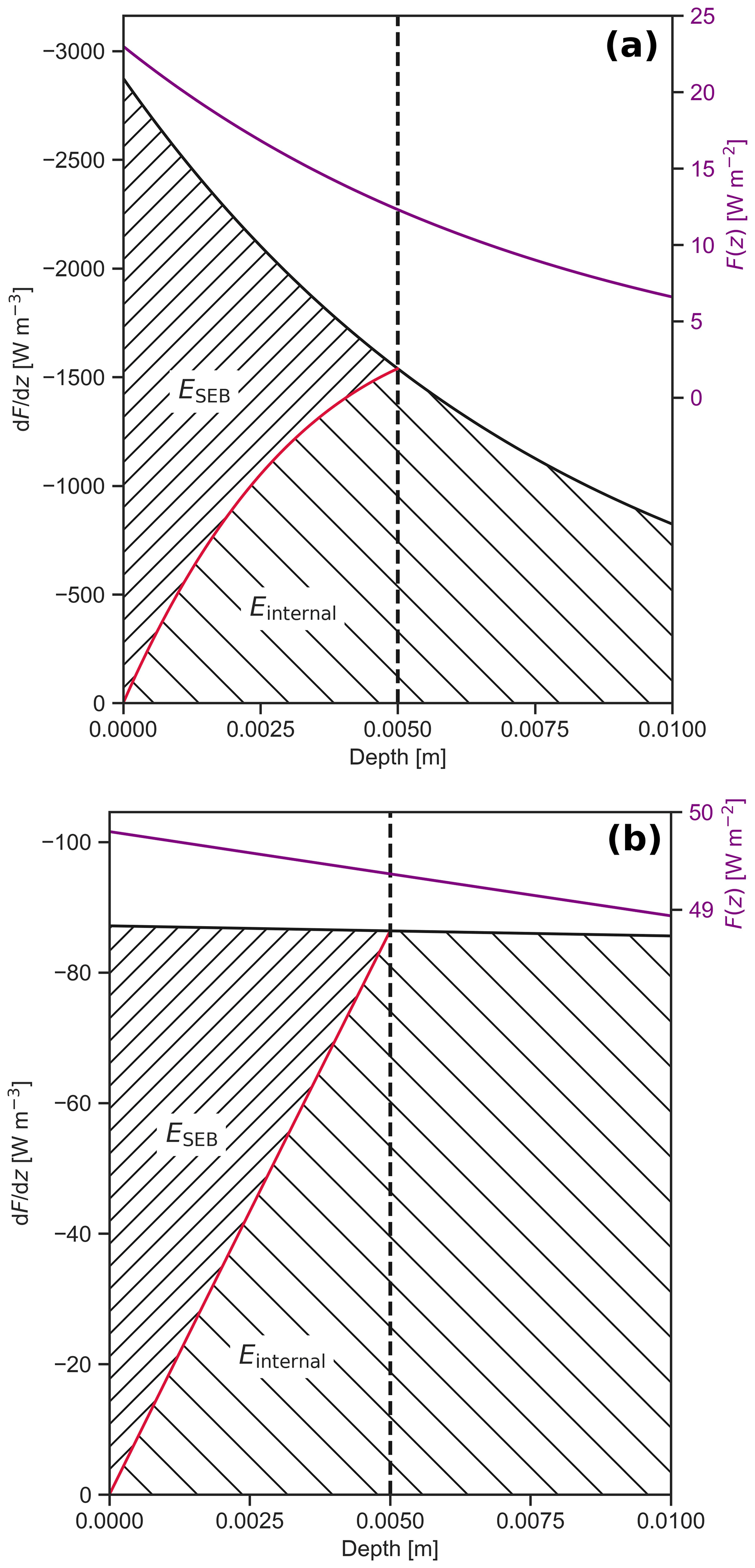
Figure 1 Net downward shortwave radiation F(z) (purple), $\mathrm{d}F\left(z\right)/\mathrm{d}z$; absorbed energy contributing to the SEB (E_SEB), indicated by the area above the red curve with dense hatches; and internal energy absorption (E_internal), indicated by the area under the red curve with sparse hatches, as a function of depth for (a) a fresh snow layer and Rp3's spectral band 6 (778–1242 nm) and (b) an ice layer for band 4 (442–625 nm). The vertical dashed line shows the 5 mm skin layer equilibration depth (SLED). Here, we assume typical net downward shortwave radiation at the surface and τ=0.008 m for panel (a) (Meirold-Mautner and Lehning, 2004) and τ=0.56 m for panel (b) (Cooper et al., 2020). All absorbed energy beyond z_sled is internal.

2.4 RACMO2 simulations

In this study, we test Rp3 on a 11 km grid for the GrIS and its immediate surroundings between 2006 and 2015, using September 2000 to December 2005 as spinup. At the lateral boundaries, Rp3 is forced with ERA-Interim data (Dee et al., 2011). The only impurity type considered is soot, which is homogeneously distributed for all snow and firn layers. The impact of soot is known to be underestimated, so a fixed concentration of 5 ng g⁻¹ is used, which is higher than the typical 3 ng g⁻¹ soot concentration of the interior (Chylek et al., 1992; Doherty et al., 2010; Dang et al., 2015). A spatially variable soot concentration is used for bare ice such that the Rp3 bare-ice albedos match the MODIS observations for clear-sky conditions and typical solar zenith angle (Van Dalum et al., 2020a).

The firn column, i.e, snow and ice density, thickness, temperature, optical grain radius, and water concentration, is initialized for all active layers with output of Rp2 (Noël et al., 2018b). Bare ice is identified if the continuous set of layers, counted from the bottom up, have a density larger than or equal to 899 kg m⁻³.

In order to highlight the impact of model changes, we investigate the sensitivity of various parameters by comparing the results with a run of Rp3 that is without internal energy absorption (Rp3 WIE). Rp3 WIE also covers the same period of analysis as Rp3 and Rp2, and all energy is added to the SEB. Furthermore, we investigate the sensitivity of the numerical choices in the implementation of internal heating by two sensitivity experiments, in which z_sled is set to 2.5 and 10 mm.

To determine the statistical significance of the bias between model versions or the bias with observations, we use statistical bootstrapping with a significance of 2 standard deviations.

2.5 In situ observations

Three types of measurements are used in this study: stake measurements to determine the SMB, automatic weather station (AWS) observations to evaluate the SEB, 2 m temperature (T_2 m) and 10 m wind speed (v_10 m), and subsurface temperature observations. The SMB observational data set in the GrIS ablation zone of Machguth et al. (2016) consists, among others, of data along the Kangerlussuaq transect (K-transect; Smeets et al., 2018) and data of the Programme for Monitoring of the Greenland Ice Sheet (PROMICE; Van As et al., 2011). The K-transect is located perpendicular to the ice margin at approximately 67^∘ N in southwest Greenland and includes both ablation and accumulation sites (shown in Fig. 5c). PROMICE measurement sites are positioned around Greenland but are mostly located in the ablation zone. A first-order approximation of the uncertainty of the SMB observations according to Machguth et al. (2016) is 0.2–0.4 m w.e. yr⁻¹. AWS data of both the K-transect and PROMICE are used to evaluate the SEB. Deriving energy fluxes from AWS data is not trivial and requires assumptions regarding surface roughness and sensor tilt corrections. For the K-transect, this is discussed in more detail by Smeets et al. (2018). Smeets et al. (2018) also report an uncertainty for shortwave radiation of approximately 1 %, for longwave radiation of ±5 W m⁻², for T_2 m of max ±0.5 ^∘C but usually ±0.2–0.3 ^∘C, and for V_10 m of at least ±0.2 m s⁻¹. Furthermore, subsurface snow temperature profiles from Summit are used. These temperature profiles have been measured during the summer of 2007 as part of the Summit Radiation Experiment (SURE '07) at depths of 0.02 m up to 0.10 m using thermocouples and at a depth of 0.20, 0.30, 0.50, 0.75, and 1.00 m using thermistor strings (Kuipers Munneke et al., 2009).

The majority of observations are performed outside the time window of the model run or within two grid points of the ice-sheet margin; these are dismissed, as the ice-sheet margins are not properly captured at the 11 km resolution used for these runs. For example, the modeled surface elevation above sea level for the PROMICE stations NUK-U and THU-U, both located close to the ice margin within two grid points on the RACMO2 grid, show an undesirably large elevation difference with observations: 1069 and 665 m in Rp3 versus 1120 and 760 m observed, respectively. Here, we accept only grid points with an elevation difference of 50 m or less. This limits the data set to S6, S7, S8, S9, and S10 for the K-transect; to KAN-M and KAN-U for PROMICE; and to two SMB measurement locations slightly to the northwest of S9.

For the evaluation of SMB and SEB, the two closest grid points to an observational site are selected in RACMO2 and linearly interpolated between them. Interpolation between two grid points is, however, not desirable for the analysis of subsurface processes, as the size and depth of snow layers in RACMO2 can change between two neighboring points. Instead, we use the nearest model grid point for subsurface processes.

3 Subsurface energy absorption

3.1 K-transect

Internal energy absorption of shortwave radiation is an important addition in Rp3. We illustrate the absorption of solar radiation and optical grain radius as a function of depth for the K-transect for 2012 in Fig. 2 (locations illustrated in Fig. 5c). S6 is situated in the ablation zone, and this dry region is characterized by a relatively thin fresh snowpack after winter. During June, the ice horizon quickly moves up, exposing bare ice until September. As S6 is situated in the so-called “dark zone” (Van de Wal and Oerlemans, 1994; Wientjes et al., 2011), the exposed bare ice has a high impurity concentration and a large optical grain radius, leading to extensive internal energy absorption (>25 W m⁻²) up to 15 cm deep. During the accumulation season, internal energy absorption is limited, except during sporadic melt events when the surface optical grain radius grows rapidly, allowing radiation to penetrate to deeper layers.

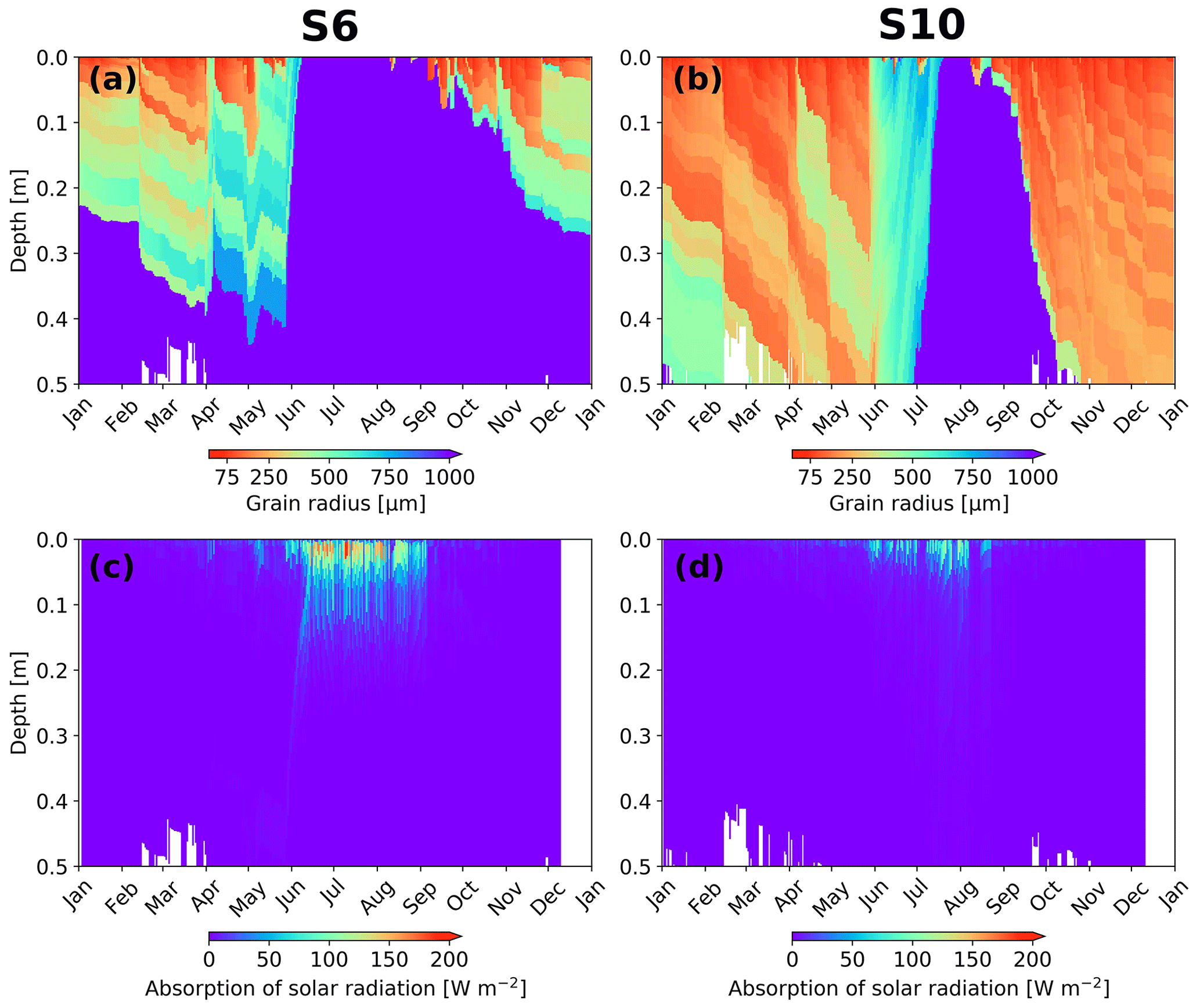
Figure 2 (a, b) Optical grain radius and (c, d) absorption of solar radiation simulated by Rp3 as a function of time and depth for the 20 uppermost snow layers for S6 (a, c) and S10 (b, d), for local solar noon (15:00 UTC) in 2012. Bare ice is indicated by an optical grain radius of 1000 µm, and white bars indicate layers beyond the 20 upper snow layers.

At S10, situated in the accumulation zone, higher winter accumulation provides a thicker snowpack at the start of the melt season than at S6. Consequently, the whole snow column only melts away during extreme melt events like in the summer of 2012 and 2019, in which bare ice surfaces for a few weeks in August (Fig. 2b). In late June and July, firn layers that are characterized by a large optical grain radius reach the surface and induce absorption of solar radiation, although less than for bare-ice conditions. The absorption, however, is limited to the upper 5 cm. Note that the formation of a thin fresh snow layer in early July diminishes internal energy absorption.

3.2 Distribution of energy

Since a fraction of the shortwave radiation is absorbed in the upper few millimeters of the snow column, not all incoming radiation contributes to internal heating (Sect. 2.3). The fraction of shortwave radiation absorbed that directly contributes to the SEB depends on wavelength and snow conditions, which is illustrated in Fig. 3. This figure shows, as an example, the absorption of energy for a summer day for a grid point at Summit in central Greenland (left bars) and S6 (hatched right bars) for the first 12 spectral bands. Bands 13 and 14 are not shown, as all energy for these bands is added to the SEB. Blue shows the energy absorbed internally and orange the energy that contributes to the SEB, with numbers above the bars indicating the percentage of surface radiation that is absorbed.

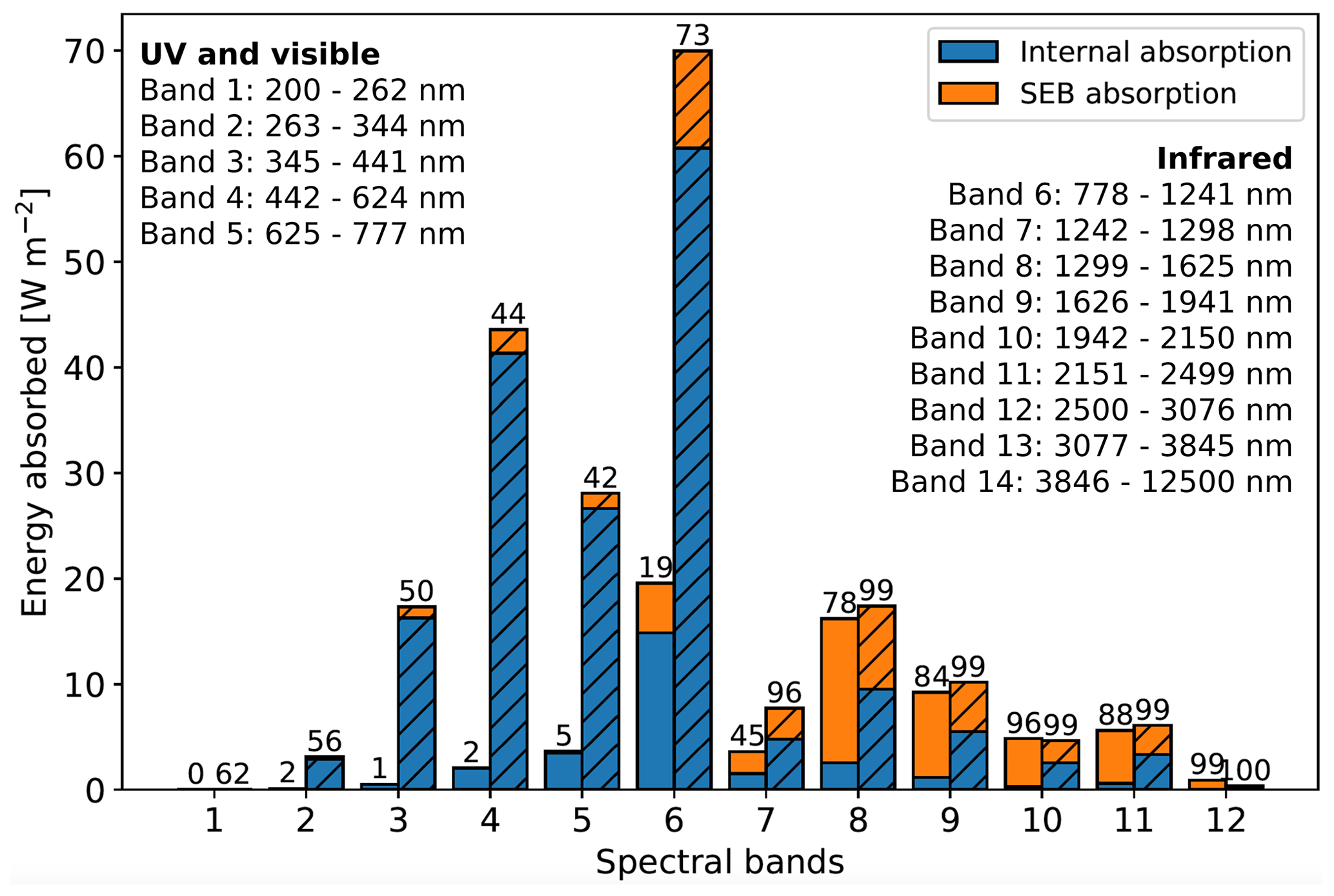
Figure 3 Energy absorbed in the snowpack during a clear-sky summer day (10 July 2007) at Summit in central Greenland (left bars) and S6 (right hatched bars) for the first 12 spectral bands of Rp3. Blue indicates the fraction of energy that is absorbed internally and orange the fraction that contributes directly to the SEB. Numbers above the bars show the percentage of radiation absorbed with respect to incoming radiation at the surface. In bands 13 and 14 (not shown), absorption at the surface is 100 %.

At Summit, almost all radiation is absorbed internally for UV and visible light (bands 1–5), but the amount of radiation that remains in the snowpack for these bands is limited. For IR radiation (bands 6–12), more absorption takes place. The attenuation length in snow is short for IR radiation (He and Flanner, 2020), leading to a strong absorption within the SLED, increasing the fraction of energy that contributes to the SEB.

S6 has bare ice at the surface for the selected day, and more radiation is absorbed in the visible light bands due to a high concentration of soot. Most notably is the large increase in energy absorbed in band 6. This is a wide band with a considerable amount of energy available; it is also especially sensitive to albedo reductions induced by an increase in optical grain radius and density, e.g., when bare ice reaches the surface (Van Dalum et al., 2019).

For bands 7 to 12, almost all incoming radiation is absorbed at S6 due to the large optical grain radius and density. Compared to Summit, a smaller fraction of energy contributes to the SEB for these bands. As the grain size has increased more strongly than the density at S6 compared to the snowpack at Summit, the number of grains in the SLED is therefore lower. In other words, the snowpack at S6 misses a scattering fresh snow top layer, hence increasing the chance of near-IR radiation to penetrate through the SLED without being absorbed. This effect is less pronounced for visible light, as the SLED is so small that visible light travels in and out virtually without loss, especially if the soot concentration is as low as that at Summit.

4 Temperature experiments

Compared to observations, the 2 m air temperature difference is only small (Table 1 and Fig. B1). The impact of internal energy absorption on the subsurface temperature, however, is larger for various locations in winter and summer and is discussed in this section. We also compare the results with Rp3 WIE. Furthermore, we discuss the 10 m snow temperature (T_10 m). We also investigate the impact of z_sled on the subsurface temperature, which is shown in Appendix B, Fig. B2.

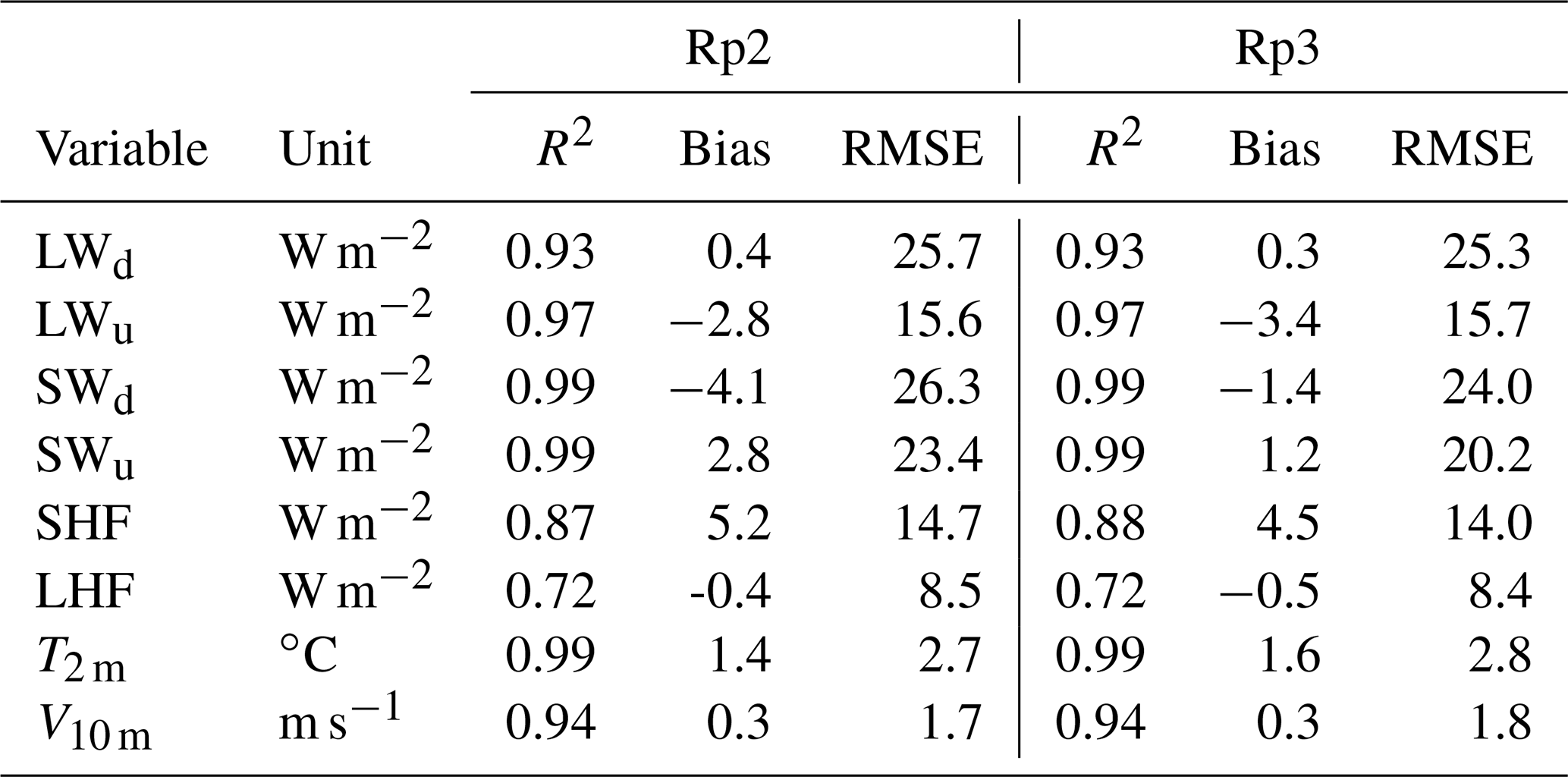
Table 1 Statistics of the daily-averaged Rp2 and Rp3 SEB components, atmospheric 2 m temperature (T_2 m), and 10 m wind speed (V_10 m) compared to in situ observations between 2006 and 2015. Data include S6, S9, and S10 (S10 is not available for T_2 m and V_10 m) of the K-transect and KAN-U and KAN-M of PROMICE. The determination coefficient (R²), root-mean-square error (RMSE), and bias are shown.

4.1 Subsurface temperature

First, we analyze the impact of internal energy absorption on subsurface snow temperatures. Figure 4 shows the subsurface temperature profiles for Rp2, Rp3, and Rp3 WIE for S6 and Summit for a winter (Fig. 4a) and a summer day (Fig. 4b). The figure also shows an example of a melt event in the accumulation zone of southeast Greenland and compares it with a melt event at S6 (Fig. 4c). All locations are shown in Fig. 5c. As the modeled temperature is not interpolated between layer mid-points, the stepwise temperature profiles indicate individual model layers. Rp3 generally has thinner snow layers, leading to a higher vertical resolution, which is especially relevant close to the surface. As Fig. 4 only shows the upper 20 snow layers, the temperature curve of Rp3 therefore does not reach as deep as Rp2.

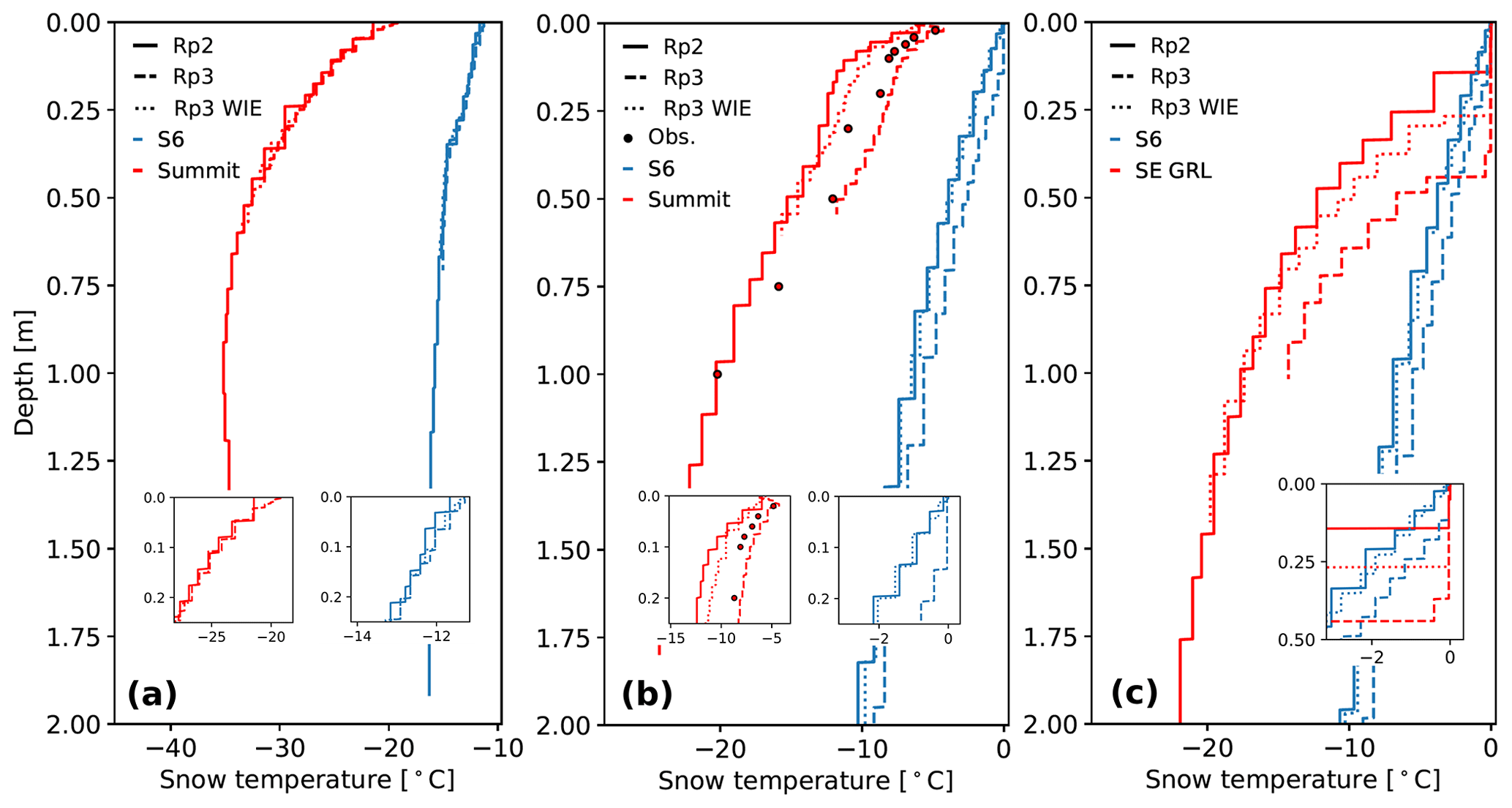
Figure 4 Subsurface temperature profiles for the 20 upper snow layers of Rp2, Rp3, and Rp3 without internal energy absorption (WIE) and observations (Obs.) for S6 and Summit for (a) a winter day (29 January 2007) and (b) a summer day (10 July 2007) at 15:00 UTC. No observations are available for Summit on this winter day. (c) Subsurface temperature profiles for a location in the accumulation zone of southeast Greenland (SE GRL, star in Fig. 5c) and S6 during a melt event (22 June 2012, 15:00 UTC). The insets show the results of the upper layers in more detail.

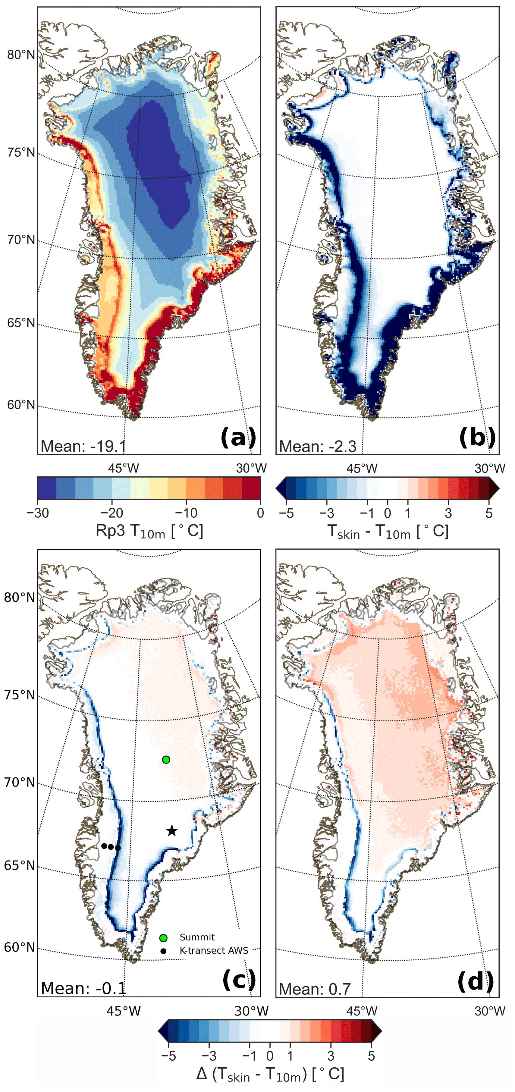
Figure 5 (a) Temperature at 10 m depth (T_10 m) at the end of the simulation (31 December 2015) for Rp3; (b) averaged yearly mean (2006–2015) skin temperature (T_skin) difference with T_10 m for Rp3, with positive values indicating that T_skin is larger than T_10 m; (c) difference between Rp3 and Rp2 for T_skin−T_10 m. The dots in the southwest are the locations of the K-transect AWS stations, from left to right: S6, S9, and S10. KAN-U and KAN-M of the PROMICE data set are located close to S10 and between S6 and S9, respectively, but are not shown separately. Subsurface temperature profiles are available for Summit (green dot). The star indicates a location that is discussed in Sect. 4.1. (d) The difference between Rp3 WIE and Rp2 for T_skin−T_10 m. In panels (c) and (d), a positive value indicates that the T_skin−T_10 m has become larger compared to Rp2.

During a typical winter day (Fig. 4a, with a T_2 m of −11 and −18 ^∘C in Rp3), the temperature profiles are similar for both S6 and Summit. Internal heating is limited, as only a small amount of radiation reaches the surface and both sites are covered with fine-grained fresh snow layers. We observe only changes in the first upper centimeters, with thinner snow layers and higher temperatures in Rp3.

During a typical summer day (Fig. 4b, with a T_2 m of 5 and −8 ^∘C in Rp3), internal energy absorption has a clear impact on subsurface temperatures. For S6, melting occurs in multiple layers, reaching to a depth of about 14 cm, which coincides approximately with depths at which absorption of solar radiation is still relevant (Fig. 2c). With the addition of internal heating, the temperature of deeper layers is raised as internal heat cannot dissipate as easily as on the surface. Higher subsurface snow temperatures make the snowpack more susceptible to internal melt, thus increasing the vertical melt extent. Note that all melting layers are still connected to the surface, effectively reducing it to a single melt layer. The impact of internal heating is also illustrated by the similar temperature profiles of Rp3 WIE with respect to Rp2.

For Summit, colder conditions prevail during summer. Compared to Rp2, the subsurface temperatures of Rp3 are considerably higher (up to 5 ^∘C) and match the observations better but are slightly overestimated in the upper 10 cm. Rp3 WIE shows lower temperatures similar to Rp2, leading to a cold bias with the observations. The temperature decline with depth, however, is more gradual for Rp3 WIE compared to Rp2. Adding internal energy absorption increases the ability of RACMO2 to reproduce realistic subsurface temperature profiles for Summit.

Figure 4c shows the subsurface temperature profiles during a melt event in the accumulation zone of southeast Greenland (SE GRL, star in Fig. 5c) and for S6. The figure illustrates that melting point is reached up to a greater depth for the accumulation point in SE GRL than S6 (0.36 and 0.18 m depth, respectively). This can be understood by surface melt percolating through snow to deeper layers, warming the subsurface. In ice at S6, meltwater can only percolate downwards through pores that are generated by internal melting. The snowpack in SE GRL, on the other hand, consists of various layers of relatively fresh snow and firn where meltwater can easily percolate, similar to the snowpack illustrated for S10 in May in Fig. 2b. A larger vertical melt extent is therefore expected for this grid point. Moreover, the addition of internal heating enhances subsurface temperatures even more, further increasing the vertical melt extent. As a warmer snowpack is more prone to melting, more melt events are expected to occur in the accumulation zone like in SE GRL. This is discussed in Sect. 6.1.

We also investigate the sensitivity of the subsurface snow temperature to the skin layer equilibration depth z_sled, which we introduced in Sect. 2.3 and set to 5 mm using scale analysis. Underestimating z_sled leads to an overestimation of internal heating, as not enough heat diffuses to the surface within the model time step, trapping too much heat beneath the surface. Increasing z_sled only has a limited effect on the subsurface temperature (Appendix Fig. B2). As expected, lowering z_sled results in too much internal heating and raises the snow temperature, illustrating that an underestimation of z_sled should be avoided.

4.2 Snow temperature at 10 m depth

In the absence of melt and refreezing, the T_10 m is regarded as a good proxy of the mean annual surface temperature (Loewe, 1970). Here, we analyze whether this assumption is true given the observed impact of radiation penetration on summer subsurface temperatures. Figure 5 shows the averaged yearly mean T_10 m at the end of the simulation for Rp3 (Fig. 5a), the difference between the average skin temperature (T_skin) and T_10 m (Fig. 5b) and the T_skin−T_10 m difference for Rp3 and Rp3 WIE with respect to Rp2 (Fig. 5c and d, respectively).

In the interior, the difference between T_skin and T_10 m is small (<0.5 ^∘C) for Rp3, illustrating that T_10 m is indeed a good proxy of the mean annual surface temperature for this region. For Rp3, T_skin−T_10 m is comparable to Rp2 (Fig. 5c); for Rp3 WIE, however, it is considerably larger (often >2 ^∘C, Fig. 5d). As all solar energy is absorbed at the surface for Rp3 WIE and the albedo is slightly lower compared to Rp2, T_skin is consequently increased while the energy that reaches 10 m depth is decreased, thus lowering T_10 m. In other words, Fig. 5d highlights the importance of radiation penetration.

In the percolation zone, the difference between T_skin and T_10 m is larger (more than −5 ^∘C, Fig. 5b), owing to latent heat being released upon refreezing. Consequently, T_10 m is not representative for the surface temperature in this zone. There are also large differences in southeast Greenland, which is characterized by firn aquifers that keep the deeper snow temperature near the melting point year round.

To conclude, T_10 m is a good measure for the surface temperature, except close to the ice-sheet margin in the southeast and the percolation zone. Moreover, subsurface energy absorption reduces T_skin−T_10 m in the interior.

5 Surface energy budget

Figure 6 shows that the SEB components of Rp3 correlate generally well with observations of S6, S9, and S10 of the K-transect and KAN-U and KAN-M of PROMICE. The downward and upward longwave radiative fluxes (LW_d and LW_u) show a determination coefficient (R²) of 0.93 and 0.97, respectively, and the performance of Rp3 is similar to Rp2 (Table 1). The influence of cloud cover is captured well, with a small and insignificant bias of LW_d and a small shortwave downward radiative flux (SW_d) bias. The bias of SW_d, however, is still significant, as is determined by statistical bootstrapping, due to the large number of data points. Despite its statistical significance, note that the uncertainty in the measurements (Sect. 2.5) is larger than the bias.

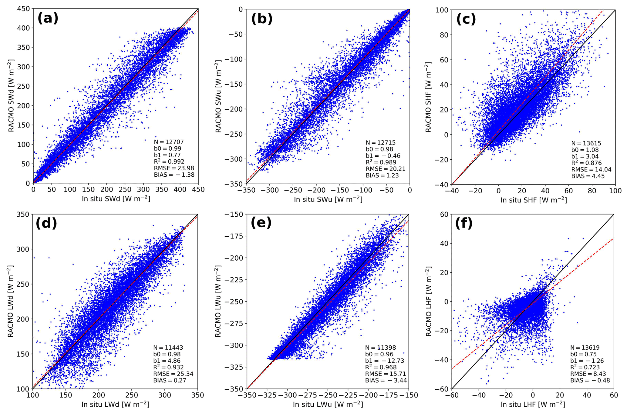
Figure 6 Daily-averaged Rp3 SEB components between 2006 and 2015 compared to in situ observations including S6, S9, and S10 of the K-transect and KAN-U and KAN-M of PROMICE for (a) downward shortwave radiation (SW_d), (b) upward shortwave radiation (SW_u), (c) sensible heat flux (SHF), (d) downward longwave radiation (LW_d), (e) upward longwave radiation (LW_u) and (f) latent heat flux (LHF). The black line is the one-to-one line, and the red line shows the orthogonal total least-squares regression of the data, with b0 the slope and b1 the intercept. Number of records (N), determination coefficient (R²), root-mean-square error (RMSE, in W m⁻²), and bias (in W m⁻²) are also displayed. In all panels, positive values imply an energy flux directed towards the surface.

The upward shortwave radiative flux (SW_u) is also in fairly good agreement with observations. The bias, however, is still statistically significant. The bias and RMSE of these fluxes have improved in Rp3 compared to Rp2 (Table 1), confirming that the albedo has improved, which is in agreement with Van Dalum et al. (2020a).

Both the sensible and latent heat flux (SHF and LHF, respectively) show a large spread and significant bias (Fig. 6c and f). While the LHF is small and contributes little to the SEB, the SHF is important to model melt events properly. The difference with observations for the 2 m temperature (T_2 m) and 10 m wind speed (V_10 m) (Table 1 and Fig. B1), however, are relatively small, and can therefore not explain the large spread of the turbulent fluxes. As is discussed in Noël et al. (2018b), the bias in SHF can be attributed to an inaccurate representation of the roughness length, especially for bare-ice conditions.

Figure 7 shows the climatology of the SEB components of in situ Rp2 and Rp3 data for S6, S9, and S10. The Rp3 and Rp2 radiative and turbulent fluxes are generally similar and agree with in situ observations. Some differences with observations are, however, still observed. The net longwave radiation (LW_n), defined as LW_d − LW_u, is lower during winter for both Rp2 and Rp3, which is mostly due to the temperature bias induced by an overestimation of SHF. No changes have been made to the cloud and SHF parameterizations in Rp3, so results similar to Rp2 are therefore expected for cloudy conditions (Noël et al., 2018b). Improving the representation of surface roughness may also improve these results.

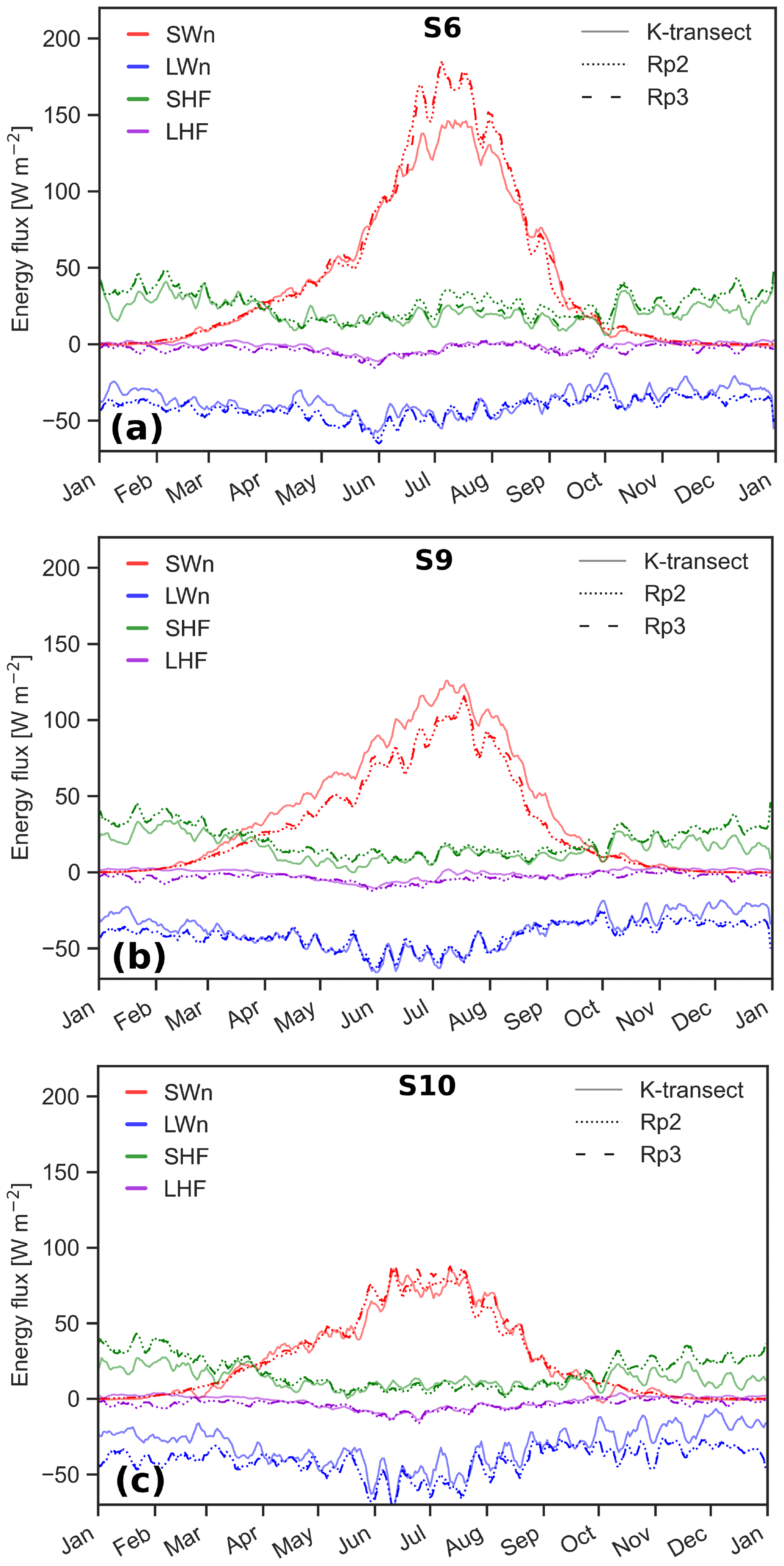
Figure 7 2006–2015 averages of the 5 d running mean SEB components for the K-transect for in situ observations, Rp2 and Rp3 at (a) S6 and (b) S9, and for 2010–2015 at (c) S10.

During summer, the SHF is overestimated by Rp2 and to a lesser degree by Rp3 for S6 (Fig. 7a). Refreezing, however, has increased for melting bare ice in Rp3 (discussed in more detail in Sect. 6.1 and Fig. 9), inducing more latent heat release, consequently heating the ice. As a result, the average skin temperature of the surface during the summer months increases and the temperature difference with the atmosphere reduces, leading to a smaller SHF. This effect is not present at S9 and S10, as bare ice rarely reaches the surface at these sites.

The net shortwave radiation (SW_n), defined as SW_d − SW_u, is similarly well represented by Rp2 and Rp3 (Fig. 7, Table 1). During summer, the differences with observations increase for S6 and S9, as both model versions overestimate SW_n due to a lower albedo compared to AWS observations. Note, however, that S6 is located in rough and inhomogeneous terrain and that the local albedo and SEB may not be representative for the entire RACMO2 grid point.

Still, some differences between Rp2 and Rp3 are worth mentioning. At the onset of the accumulation season at S6, thin snow layers form and are modeled on top of bare ice. The lack of radiation penetration and internal heating in Rp2 leads to a too rapid brightening of the surface in Rp2 and subsequently underestimated SW_n and hence melt–albedo feedbacks in early fall. Eventually, the new snow layer becomes thick enough to cover the bare ice even if radiation penetration is taken into account, and the differences between both model versions disappear. This effect is also to a lesser degree visible at S9. For S9, which is located close to the percolation zone, the albedo is overestimated for both Rp2 and Rp3. This is likely caused by an incorrect representation of the firn layer. The albedo differences are small for S10 (Van Dalum et al., 2020a). As S10 is located in the lower accumulation zone, it is typically characterized by a homogeneous thick firn layer and little melt. Consequently, SW_n is relatively similar in both model versions and is often in agreement with observations (Van Dalum et al., 2020a).

6 Surface mass balance

6.1 Comparison with RACMO2.3p2

Figure 8a shows the annual average 2006–2015 SMB for Rp3. The absolute and relative difference with Rp2 (Rp3 − Rp2) is shown in Fig. 8b and c, respectively. Figure 8b also shows the statistical significance. Almost all SMB changes are significant with respect to the inter-annual variability; only some of the smaller changes in the interior are insignificant. Integrated over the ice sheet, the SMB increases by 17.0 mm w.e. yr⁻¹ (29.1 Gt yr⁻¹) or 9.7 %. The annual difference between Rp3 and Rp2 and significance for melt, refreezing, and runoff are shown in Fig. 9. Changes in modeled precipitation, sublimation, and drifting snow erosion are not shown, as these processes are not significantly affected by the changes implemented in Rp3, and the differences are on average below 1.1 mm w.e. yr⁻¹.

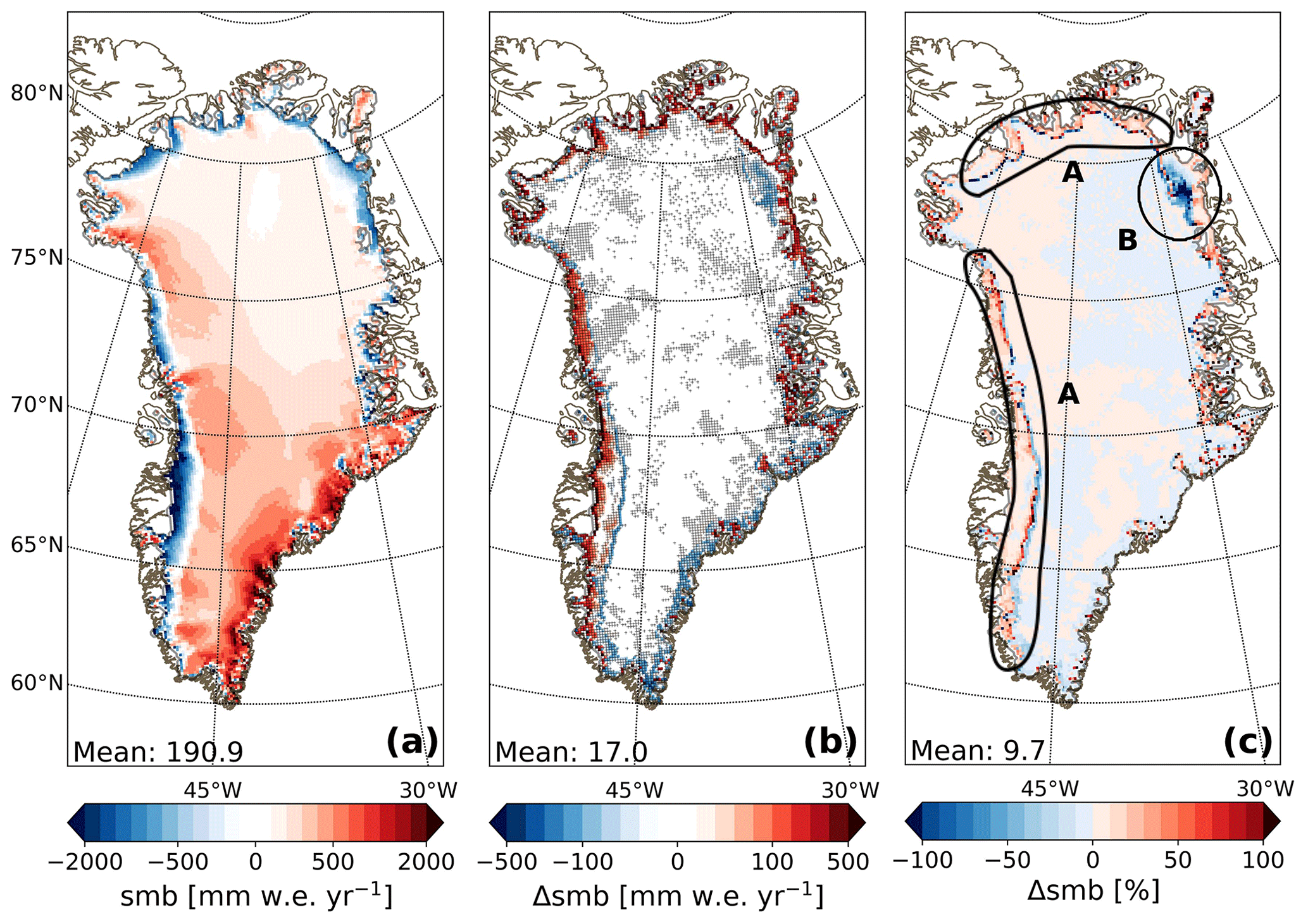
Figure 8 (a) Annual average surface mass balance between 2006 and 2015 for Rp3, with a linear color scale with a step size of 100 mm w.e. yr⁻¹ between −500 and 500 and 500 mm w.e. yr⁻¹ elsewhere. (b) SMB difference (Rp3 − Rp2). A linear color scale with a step size of 100 mm w.e. yr⁻¹ between −500 and −100 and between 100 and 500 mm w.e. yr⁻¹ is used and 20 mm w.e. yr⁻¹ elsewhere. The hatched areas show statistical significance. (c) The relative difference between Rp3 and Rp2. Patterns A and B are discussed in the text.

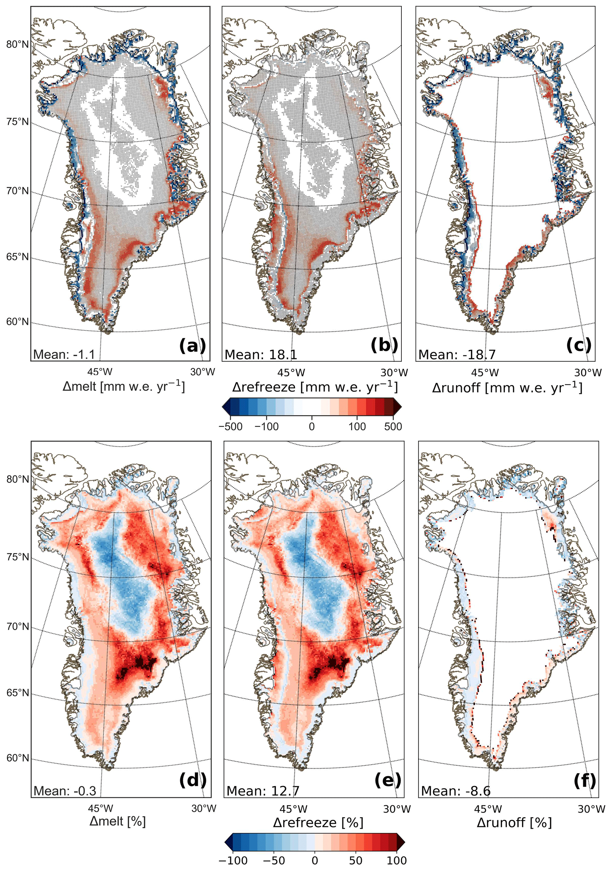
Figure 9 Annual average difference (Rp3 − Rp2) for 2006–2015 for (a) melt, (b) refreezing, and (c) runoff in mm w.e. yr⁻¹, with the same color scale as in Fig. 8b, and average relative difference for (d) melt, (e) refreezing, and (f) runoff. The hatched areas in panels (a)–(c) show statistical significance.

In the interior, a significant melt increase is observed in northeast and south Greenland (Fig. 9a). This is mostly caused by albedo changes but also partly by radiation penetration inducing internal heating. As is discussed in Sect. 3, internal heating raises the subsurface temperature and increases melt. Because all melt refreezes in the snowpack, these changes do not affect the local SMB (Fig. 9b and c). Refreezing, however, changes the structure of the snowpack, inducing more energy absorption and higher snow temperatures, leading to more melt.

The outer rim of the ice sheet, except in the southeast, is characterized by a strong and significant SMB increase (Fig 8). In Rp2, the ice mask is not projected properly on the bare-ice albedo field, causing the outermost glaciated grid points to be contaminated with tundra albedo. The albedo of the outermost glaciated grid points is therefore as low as 0.3, inducing too much melt and runoff. The impact of this artifact is mitigated for higher resolutions and is solved in Rp3 (Van Dalum et al., 2020a), lowering the melt and runoff and increasing the SMB. In the southeast close to the ice-sheet margin, this issue is absent, as at this low resolution the number of grid points for which bare ice reaches the surface is limited. Melt is slightly higher and refreezing is similar to Rp2 for this region, resulting in more runoff.

The lower ablation area of the GrIS in the southwest experiences a strong increase in refreezing (Fig. 9b), while the SMB difference is limited. Refreezing is enhanced by the introduction of radiation penetration. In Rp3, subsurface melting of ice creates pore space (Sect. 2.1.1) and consequently increases the meltwater retention capacity. In Rp2, no retention capacity remains once bare ice reaches the surface, limiting refreezing in the shallow winter snowpack. Additionally, some regions in the southwest show a melt increase, which is induced by, on average, a slightly lower albedo in Rp3 (Van Dalum et al., 2020a). As a result, the increase in melt and refreezing balance out, leading to an insignificant runoff difference for most of the southwestern ablation zone (Fig. 9); hence the SMB changes little (Fig. 8b).

In Rp3, melt has increased in the percolation zone, and most of the additional meltwater refreezes locally. Close to the equilibrium line, however, the meltwater buffering capacity is exceeded due to the addition of meltwater, and runoff occurs, lowering the SMB (pattern A in Fig. 8c). Similarly, in the upper ablation zone, where the winter snow cover lasts long during summer, enhanced melt leads to reduced refreezing, as the refreezing capacity is consumed faster.

The northeast shows a large area with reduced SMB (pattern B in Fig. 8c). This region is characterized by dry conditions, resulting in a thin winter snow layer that melts away quickly in spring, exposing bare ice. Due to the low albedo of bare ice and radiation penetration, the ice temperature is raised, leading to melt in multiple model layers reaching greater depths and prolonging the melt season (as is discussed in Sect. 4.1), consequently enhancing melt and runoff (Fig. 9a, c, d, and f). Furthermore, it usually takes several weeks after the ablation season ends for fresh snow layers to grow to a thickness of over 10 cm. During this time, some radiation can still reach bare-ice layers, lowering the albedo and inducing more energy absorption.

The larger melt extent for the star in southeast Greenland (Fig. 4c, star in Fig. 5c) is in agreement with Fig.  9d and e, where we see more melt and refreezing for this grid point. As the elevation of this location is too far above sea level, no runoff is modeled and all meltwater refreezes locally. Even though the melt and consequent refreezing are still small and do not alter the SMB, they do change the snow structure.

To summarize, averaged over the ice sheet, annual melt has barely changed, i.e., −1.1 mm w.e. yr⁻¹ (−1.88 Gt yr⁻¹, −0.3 %), compensating for the increase in melt in south Greenland with the reduced melt at the margins. The annual runoff, on the other hand, is lowered by −18.7 mm w.e. yr⁻¹ (−32.0 Gt yr⁻¹, −8.6 %) while annual refreezing has increased by 18.1 mm w.e. yr⁻¹ (31.0 Gt yr⁻¹, 12.7 %). By percentage, melt and refreezing have increased considerably in the interior of the ice sheet, except for a large area in the center (Fig. 9d and e). This is discussed in more detail in Sect. 6.2. No runoff is modeled in the interior (Fig. 9c and f), as meltwater refreezes locally. Around the K-transect, the increase in refreezing consequently lowers the modeled runoff. Significant runoff increase is modeled in A and B.

6.2 Cloud cover and melt

For a large area of the central GrIS, annual melt and refreezing have decreased by percentage (Fig. 9d and e). Melt events in this region, although rare, are almost always associated with above-average cloud cover (Fig. 10a), reducing the amount of SW radiation that reaches the surface. In general, the albedo of Rp3 is lower than Rp2 for this region (Van Dalum et al., 2020a), but for cloudy conditions and during melt events, the albedo of Rp3 is higher (Fig. 10b), leading to less energy absorbed in the snowpack and subsequently less melt and refreezing. This albedo increase is mostly caused by the changing spectral distribution of irradiance during cloudy conditions, as relatively more of the irradiance is ultraviolet (UV) and visible light, for which the albedo is high, and relatively less is IR radiation, for which the albedo is low (Dang et al., 2015; Van Dalum et al., 2019; Warren, 2019). A large fraction of UV and visible radiation is absorbed internally (Fig. 3), heating subsurface layers that can potentially increase melt. This effect, however, is not enough to mitigate the reduced irradiance and higher albedo, and therefore less melt is modeled. To summarize, cloud cover during melt events changes the spectral distribution of shortwave radiation at the surface, shifting more towards shorter wavelengths (UV and visible light). As the albedo is higher for these shorter wavelengths, which is now properly modeled in Rp3, less energy is available for melt. Note that the total amount of melt modeled for this region in the central GrIS is on average very small (2 mm w.e. yr⁻¹) compared to ablation areas (e.g., 2500 mm w.e. yr⁻¹ at S6).

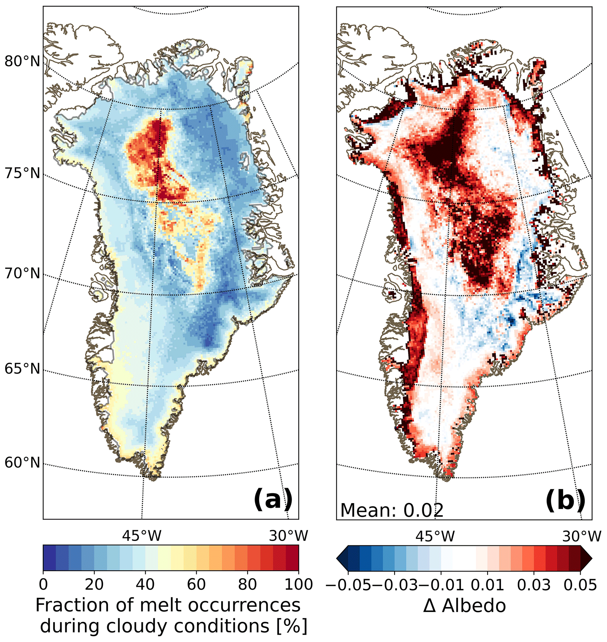
Figure 10 (a) Fraction of melt occurrences during cloudy conditions for Rp3 and (b) the albedo difference (Rp3 − Rp2) during melt events and cloudy conditions. A minimum vertically integrated cloud content of 0.05 kg m⁻² is required to be considered cloudy, and a minimum melt rate of 1 mm w.e. d⁻¹ is required to be considered a melt event. Using this low threshold should guarantee that all major melt events are included (Fettweis et al., 2011; Fausto et al., 2016). All data are averaged between 2006 and 2015.

6.3 SMB observations

Figure 11 shows the annual SMB of Rp3 and Rp2 with respect to various SMB observations. The determination coefficient, root-mean-square error (RMSE), and bias with respect to observations are also shown. A slightly higher SMB is modeled for Rp3 compared to Rp2. The bias with observations for Rp3 is −0.031 m w.e. yr⁻¹ (−2.67 %) and for Rp2 −0.091 m w.e. yr⁻¹ (−7.54 %), but both are statistically insignificant. The differences with observations are particularly relevant for the measurement sites in the lower ablation zone (S6, squares in Fig. 11) and are caused by increased refreezing in Rp3 (Fig. 9b). Note that the spread is higher for the ablation zone, illustrating that the large temporal variability is not always captured properly with this resolution in RACMO2. Increasing the resolution might improve the modeled estimates for the locations close to the ice margin.

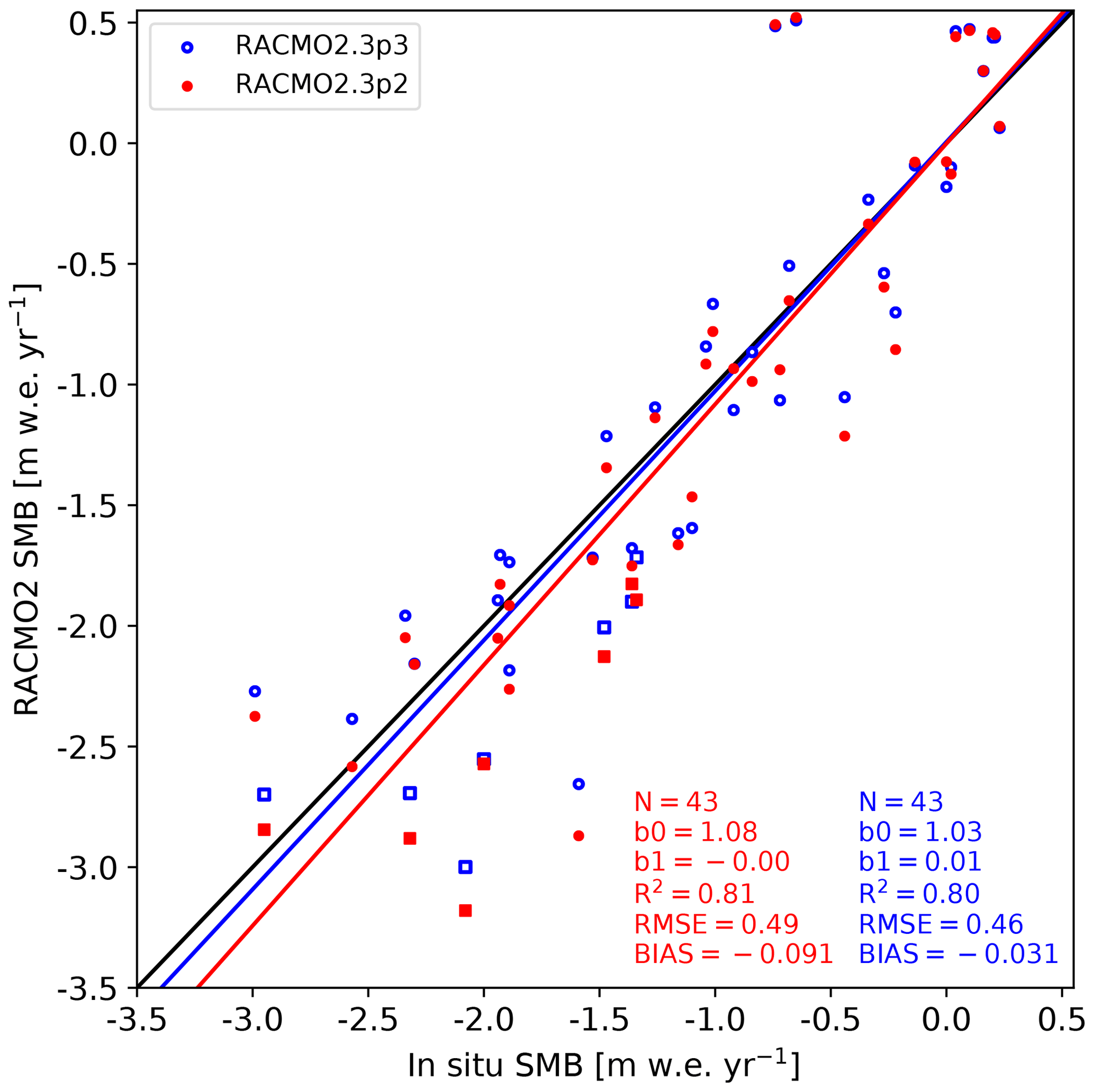
Figure 11 Surface mass balance along the K-transect in Rp3 (blue) and Rp2 (red), compared to annual in situ stake observations (m w.e. yr⁻¹). Measurements are taken between 2006 and 2015, with each dot representing 1 year. Only observations at least two grid points away from the ice margin in the RACMO2 grid are selected for evaluation (locations are shown in Fig. 8b). The black line is the one-to-one line, and the red and blue line show the linear regression of the data, with b0 the slope and b1 the intercept. Number of records (N), determination coefficient (R²), root-mean-square error (RMSE, in m w.e. yr⁻¹), and bias (in m w.e. yr⁻¹) are also displayed. Results for S6 are shown with squares.

6.4 SMB without internal energy absorption

Finally, we discuss the impact of radiation penetration on the SMB and analyze its components by comparing Rp3 with Rp3 WIE. Figure 12 shows the differences in the annual SMB, melt, and refreezing between the two simulations. Note that in Rp3 WIE radiation penetration is still used to determine the albedo, but all absorbed shortwave radiation is added to the SEB.

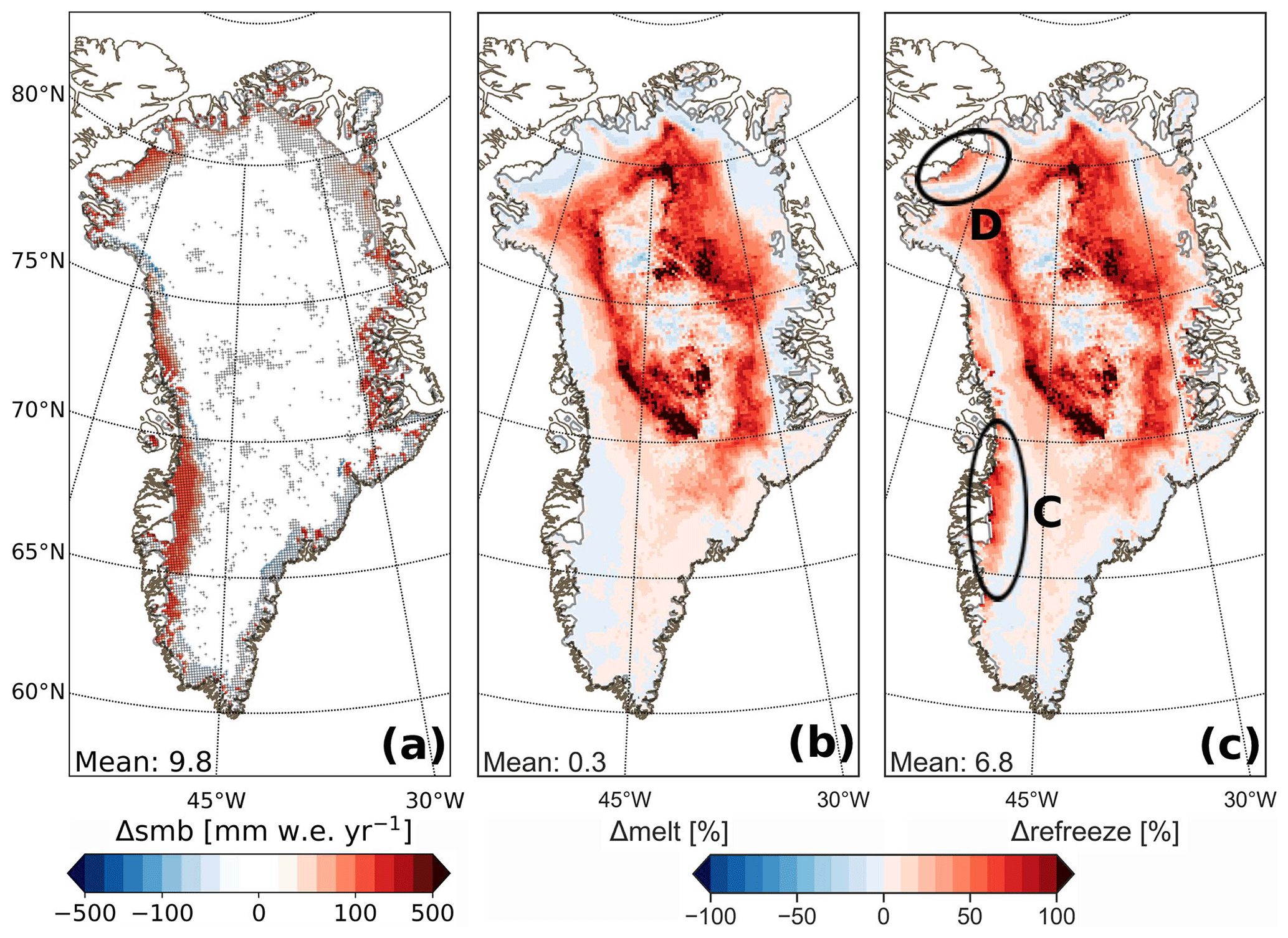
Figure 12 The 2006–2015 annual average difference between Rp3 and Rp3 WIE (Rp3 − Rp3 WIE) for (a) the SMB in mm w.e. yr⁻¹ and by percentage for (b) melt and (c) refreezing. The same color scale is used as in Fig. 8b for panel (a) runoff. The hatched areas in panel (a) show statistical significance.

The SMB is higher for Rp3 in most of the ablation zone (Fig. 12a), in particular in the southwest (area C of Fig. 12c), where we observe a relatively small melt decrease (Fig. 12b). More importantly, however, is that internal radiative heating in Rp3 increases refreezing in the ablation zone (Fig. 12c), especially in the southwest, but also in the northwest and northeast (areas C, D of Fig. 12c, and B of Fig. 8c, respectively), reducing modeled runoff. Hence, the SMB of Rp3 WIE is lower than Rp3 for these areas. This increase in refreezing in Rp3 is likely realistic, as bare ice does have retention capacity for water, and refreezing can occur overnight, while in Rp2 melting bare ice essentially remains dry as meltwater is removed instantaneously.

In the central part of the interior, the melt and refreezing differences between Rp3 and Rp3 WIE are smaller than for the surrounding areas (Fig. 12b, c). This supports the findings of Sect. 6.2, where we show that the albedo dominates the signal and not subsurface energy absorption. The differences between Rp3 and Rp3 WIE are consequently only small, as both model simulations use the same albedo scheme. For the surrounding areas, however, Fig. 12b and c show that subsurface energy absorption plays a more important role, as the difference between the model simulations for melt and refreezing increases.

In south Greenland, the melt and refreezing difference between Rp3 and Rp3 WIE is smaller than between Rp3 and Rp2 (Fig. 9d). This means that processes other than subsurface energy absorption are important here. This region is characterized by an albedo decrease due to slightly stronger snow metamorphism and slower firn–ice transition in Rp3 (Van Dalum et al., 2020a), resulting in more absorption of shortwave radiation, inducing melt and subsequent refreezing. Hence, it contributes to the differences between Rp3 and Rp2.

7 Conclusions

Regional climate models often do not explicitly account for radiative transfer in snow and ice. Therefore, we evaluated the latest version of the regional climate model RACMO2, which has an updated radiative transfer scheme that allows internal heating. In this new version Rp3, we also updated the multilayer firn module and snow and ice albedo (Van Dalum et al., 2020a), and we developed a method to distribute total absorbed shortwave radiation between the SEB and internal absorption. In this study, we assessed the modeled surface mass balance (SMB), surface energy budget (SEB), and firn and snow temperature of the GrIS.

We have run Rp3 for the GrIS for 2006–2015 using ERA-Interim data at the lateral boundaries. The modeled SMB correlates well with ablation stake measurements, and the SEB is in good agreement with AWS observations at the K-transect and for a selection of PROMICE stations. Moreover, subsurface temperature profiles show a more gradual temperature decrease with depth in Rp3 during summer in the interior, improving the agreement with observed snow temperatures at Summit, and melt reaches deeper layers in both the accumulation and ablation zone.

Compared to the previous RACMO2 version Rp2, the SMB difference is small in the interior, as any change in melt is balanced by refreezing. Close to the percolation zone near the equilibrium line, the SMB is lowered as the meltwater buffering capacity is exceeded due to the addition of melt, leading to runoff. In the ablation zone in the southwest, significantly more refreezing occurs due to pore space created in ice by melt induced by subsurface energy absorption. Finally, the SMB is higher at the very margins due to the removal of an artifact in the ice albedo of Rp2, which reduces melt. These differences are small or absent in the wet southeast, where bare ice rarely reaches the surface. For the accumulation zone of the southeast, relative differences in melt and refreezing are substantial due to subsurface energy absorption and meltwater percolation. This increased melt and refreezing often does not lead to significant SMB changes but does change the snow structure.

There is, however, still room for improvement. The resolution used in this study, i.e., 11 km horizontal resolution, is sufficient to resolve the SMB and SEB in the interior of the ice sheet but is insufficient to resolve the inhomogeneous ablation zone, especially close to the ice margin. For example, bare rock cropping out of the ice, steep slopes, or snow patches are usually smaller than the current horizontal resolution of RACMO2. More fundamentally, the ice albedo, although considerably improved in Rp3 (Van Dalum et al., 2020a), could be further improved by using a dynamic Mie-scattering theory model (Gardner and Sharp, 2010). In addition, a new impurity scheme that would allow the introduction of more impurity types and varying concentrations for each layer in space and time and would be beneficial. The turbulent fluxes could be further improved as well. We have shown that there are still some biases in the SHF and LHF, especially for areas with rough terrain like S6. A better representation of the surface roughness and the atmospheric fluxes in this complex terrain is therefore desirable (Van Tiggelen et al., 2021).

To conclude, Rp3 is capable of accurately reproducing the SMB, SEB, and (sub)surface temperature when compared to in situ observations. Differences with Rp2 are most pronounced in the ablation zone close to the ice margin, in south Greenland and close to the percolation zone. Furthermore, the snow temperature with depth is altered over the whole ice sheet due to subsurface energy absorption. The improvements made in Rp3 are especially relevant in a warming climate where the GrIS surface will typically have lower albedos and more subsurface energy absorption, thus improving RACMO2's capability of making future climate projections. This study therefore shows the necessity of radiative transfer in snow and ice for regional climate modeling of the GrIS. In a subsequent study, we will assess the ability of Rp3 to simulate albedo and melt in Antarctica.

Appendix A: Scale analysis

Using scale analysis on the heat equation, we estimate the depth heat diffusion reaches within a model time step:

$$\begin{array}{}\text{(A1)}& \begin{array}{rl}& {\displaystyle \frac{\partial T}{\partial t}}={\displaystyle \frac{k}{\mathit{\rho }{c}_p}}{\displaystyle \frac{{\partial }^{\mathrm{2}}T}{\partial z^{\mathrm{2}}}},\\ & {\displaystyle \frac{\mathrm{\Delta }T}{\mathrm{\Delta }t}}={\displaystyle \frac{k}{\mathit{\rho }{c}_p}}{\displaystyle \frac{\mathrm{\Delta }T}{\mathrm{\Delta }{z}^{\mathrm{2}}}},\\ & \mathrm{\Delta }z=\sqrt{{\displaystyle \frac{k}{\mathit{\rho }{c}_p}}\mathrm{\Delta }t},\end{array}\end{array}$$

with T the snow/ice temperature, Δz the depth scale, Δt the model time step (4 min), k the thermal conductivity, ρ the snow/ice density, and c_p the specific heat content. Using Eq. (A1) and typical values for k, ρ, and c_p (Fukusako, 1990; Sturm et al., 1997) results in Δz being on the order of 5 mm for both snow and ice.

Appendix B: Figures

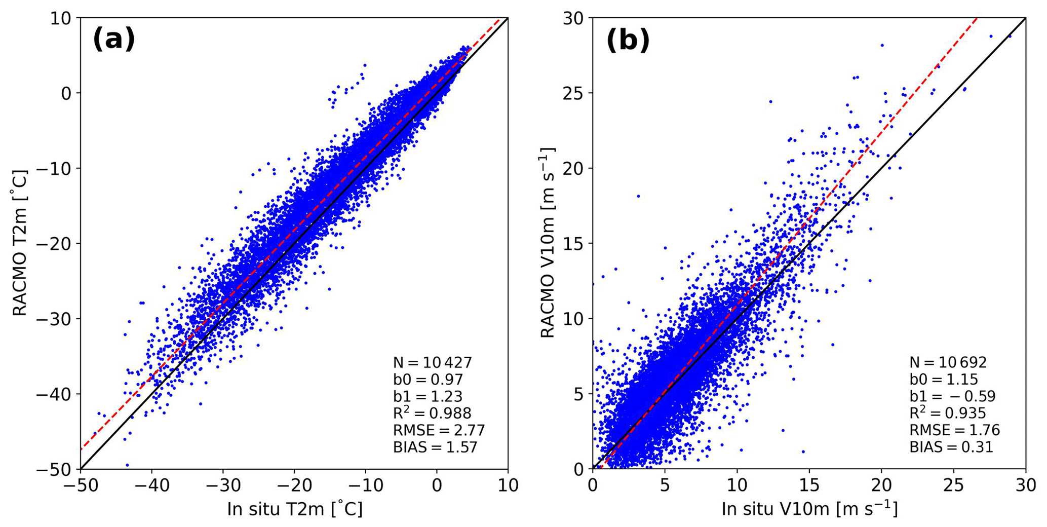
Figure B1 Daily-averaged (a) atmospheric 2 m temperature (T_2 m) and (b) 10 m wind speed (V_10 m) of Rp3 compared to in situ observations between 2006 and 2015 for S6 and S9 (S10 is not available) of the K-transect and KAN-U and KAN-M of PROMICE. The black line is the one-to-one line, and the red line shows the orthogonal total least-squares regression of the data, with b0 the slope and b1 the intercept. Number of records (N), determination coefficient (R²), root-mean-square error (RMSE, in ^∘C and m s⁻¹, respectively), and bias are displayed.

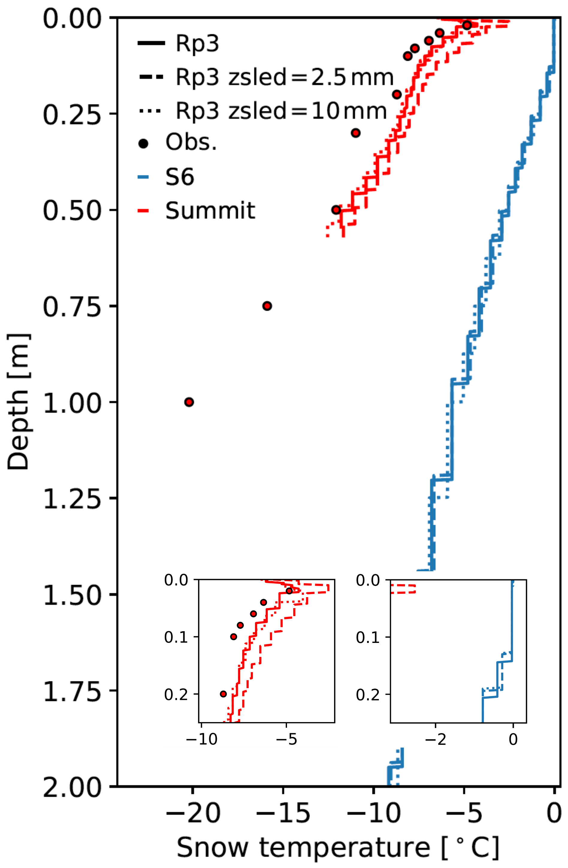
Figure B2 Subsurface temperature profiles for the 20 upper snow layers of Rp3 and Rp3 with z_sled=2.5 mm, Rp3 with z_sled=10 mm, and observations (Obs.) for S6 and Summit for a summer day (10 July 2007) at 15:00 UTC. The insets show the results of the upper layers in more detail.