Evidence for a grounding line fan at the onset of a basal channel under the ice shelf of Support Force Glacier, Antarctica, revealed by reflection seismics

Curvilinear channels on the surface of an ice shelf indicate the presence of large channels at the base. Modelling studies have shown that where these surface expressions intersect the grounding line, they coincide with the likely outflow of subglacial water. An understanding of the initiation and the ice–ocean evolution of the basal channels is required to understand the present behaviour and future dynamics of ice sheets and ice shelves. Here, we present focused active seismic and radar surveys of a basal channel, ∼950 m wide and ∼200 m high, and its upstream continuation beneath Support Force Glacier, which feeds into the Filchner Ice Shelf, West Antarctica. Immediately seaward from the grounding line, below the basal channel, the seismic profiles show an ∼6.75 km long, 3.2 km wide and 200 m thick sedimentary sequence with chaotic to weakly stratified reflections we interpret as a grounding line fan deposited by a subglacial drainage channel directly upstream of the basal channel. Further downstream the seabed has a different character; it consists of harder, stratified consolidated sediments, deposited under different glaciological circumstances, or possibly bedrock. In contrast to the standard perception of a rapid change in ice shelf thickness just downstream of the grounding line, we find a flat topography of the ice shelf base with an almost constant ice thickness gradient along-flow, indicating only little basal melting, but an initial widening of the basal channel, which we ascribe to melting along its flanks. Our findings provide a detailed view of a more complex interaction between the ocean and subglacial hydrology to form basal channels in ice shelves.

1 Introduction

Ice shelf channels (Drews, 2015), also known as channels (Alley et al., 2016), surface channels (Marsh et al., 2016) or M-channels (Jeofry et al., 2018b), are narrow (a few kilometres wide and 20–30 m deep mostly), long channels on the surfaces of ice shelves. They are often remotely detected with satellite imagery like MODIS (Moderate Resolution Imaging Spectroradiometer; Scambos et al., 2007) or Landsat 8. These channels are a surface expression of a sub-ice-shelf channel (Le Brocq et al., 2013), also known as a basal channel (Marsh et al., 2016; Alley et al., 2016, 2019) or U-channel (Jeofry et al., 2018b), most often aligned with the ice flow direction but occasionally migrating across the ice flow direction. They typically are a couple of hundred metres high and a few kilometres wide (Jeofry et al., 2018b; Drews et al., 2017). As locations of thinner ice these channels can induce ice shelf fracturing (Dow et al., 2018). Thus ice shelf channels potentially influence ice shelf stability, which in turn provides stability of the ice sheet through the buttressing effect (Thomas and MacAyeal, 1982; Fürst et al., 2016). Alley et al. (2016) categorized three types of basal channels: (1) ocean-sourced channels that do not intersect with the grounding line, (2) subglacially sourced channels that intersect the grounding line and coincide with modelled subglacial water drainage, and (3) grounding-line-sourced types that intersect the grounding line but do not coincide with subglacial drainage of grounded ice. In the following we will use the term surface channel and basal channel to make a clear separation.

In the grounding line area of the Antarctic Ice Sheet, the location of modelled channelized meltwater flow often coincides with basal channels (and its surface expression, the surface channel) (Le Brocq et al., 2013). This suggests subglacial drainage contributes to the formation of basal channels. According to Jenkins (2011) subglacial meltwater entering the ocean cavity at the grounding line forms a plume entraining warmer ocean water and causes increased subglacial melt beneath the ice shelf, which drives the further evolution of channel geometry. This hypothesis is often supported by an idealized and conventional geometry of the sheet–shelf transition at the grounding line area: the ice–water contact (the underside of the ice shelf) rises steeply beyond the grounding line, thus allowing fresh water influx to form uprising melt plumes and then levelling out more horizontally further downstream (Le Brocq et al., 2013; Drews et al., 2017).

Drews et al. (2017) linked the formation of a basal channel to a potential esker upstream of the grounding line, noting that the channel dimensions are an order of magnitude larger then eskers in deglaciated areas. However, Beaud et al. (2018) found that eskers are more likely to form under land-terminating glaciers. Jeofry et al. (2018b) concluded that the basal channels at Foundation Ice Stream were initially formed by hard-rock landforms upstream of the grounding line. Bathymetric surveys at different locations showing hard bedded landforms of similar dimensions as the basal channels confirmed this as a possibility. Alley et al. (2019), however, argued that shear margins of ice streams develop surface troughs continuing downstream of the grounding line. Once afloat, these surface troughs lead to the formation of basal channels during adjustment to hydrostatic equilibrium, thereby forming a basal channel. Thus a channelized warm water plume is likely to incise a basal channel, forming observed polynyas at the ice shelf front. Both hard-rock landforms and surface troughs at shear margins of ice streams seem to cause basal channels. Unfortunately, key observations are often missing, e.g. on the type of material and structure of the bed upstream of a basal channel.

From noble gas samples at six locations beneath the Filchner Ice Shelf, Huhn et al. (2018) estimated a total freshwater influx of 177±95 Gt a⁻¹, entering the Filchner Ice Shelf. At one location, downstream of Support Force Glacier (SFG), the noble gas sample indicated crustal origin and thus that part of the freshwater influx has a grounded subglacial origin. We also know that the west side of SFG, where a surface channel is present, coincides with modelled channelized subglacial drainage (Le Brocq et al., 2013; Humbert et al., 2018). Thus we have good reason to assume there is a subglacial drainage channel present at SFG.

Most field observations of surface channels and basal channels come from satellite imagery or airborne or ground-penetrating radar. Although airborne radar gives a good impression of the shape of the ice shelf at larger scales, its trace distance is large (on the order of 10 m) and primarily registers nadir reflections. The narrow aperture thus provides only limited insight into the precise geometry of the channel, especially steep structures like the flanks of the basal channel. In addition, radar signals typically do not penetrate below wet ice-bed contacts, making it hard to determine the nature of subglacial material: is water exclusively present on hard bedrock or does the substrate also consist of sediments?

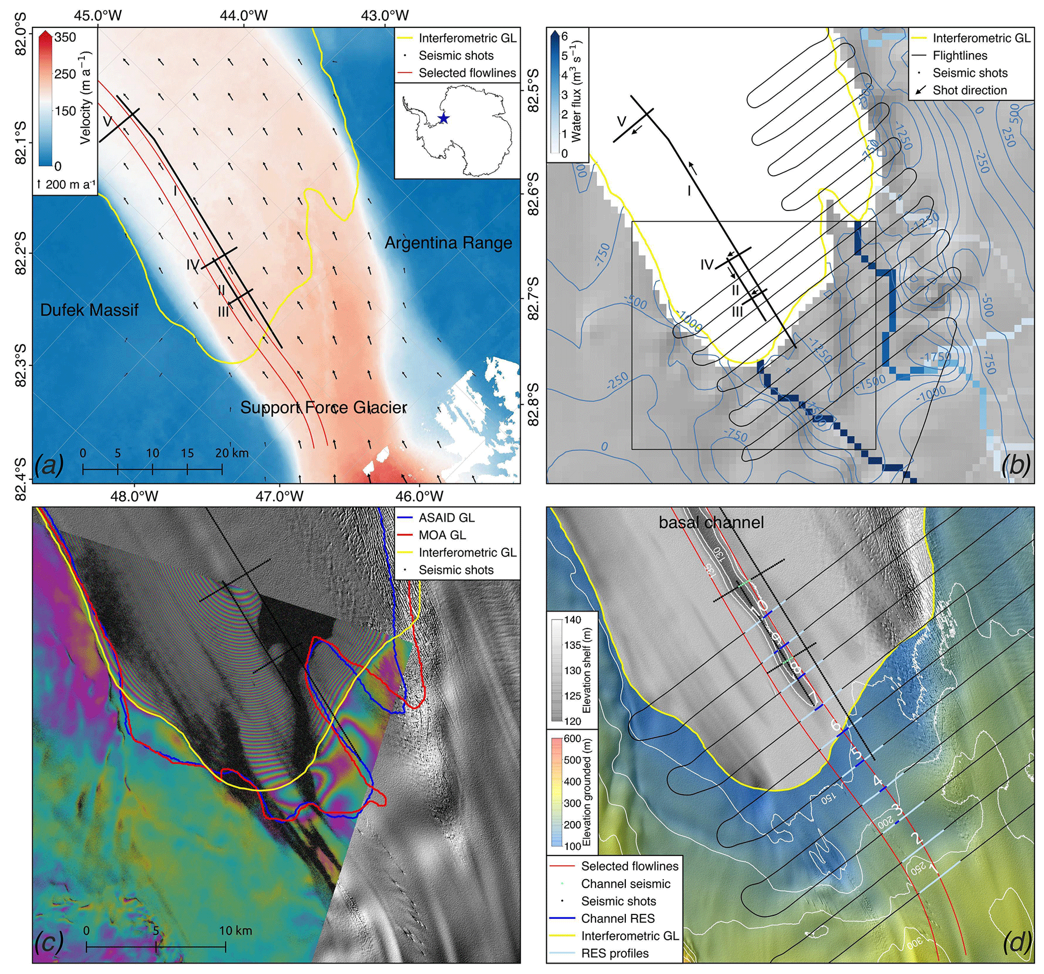
Figure 1 Location of the seismic and airborne radar surveys of the grounding line (GL) area of Support Force Glacier (SFG). (a) Ice surface velocity map of the survey area. The seismic profiles are marked by black dots, along-flow profiles I and II, and across-flow profiles III, IV and V. Two flow lines are marked in red and the GL in yellow. Inset: location of SFG in Antarctica. (b) Modelled subglacial water routing flux at SFG from the static hydrological potential. Shown are our updated bedrock compilation, a combination of BEDMAP2, and the collected airborne radar survey (thin black looping line). The shooting direction of the seismic profiles is shown by the arrows. The black rectangle marks the subregions of (c) and (d). (c) Three proposed GLs are marked in blue (ASAID; Bindschadler et al., 2011), red (MODIS; Scambos et al., 2007) and yellow (based on interferometry). The background is a shaded version of the 8 m Reference Elevation Model of Antarctica (REMA; Howat et al., 2019) overlaid by a TerraSAR-X interferogram used in the delineation of the grounding line. (d) The topography of the ice shelf (grey) indicates the surface channel. Numbered are loops 1 to 10 of the airborne radar data. Loops 1 to 5 are on the grounded part, loop 6 is at the GL and loops 7 to 10 are on the shelf. In light blue we see the radar profiles shown in Fig. 5. In green (seismic profiles) and dark blue (radar) we see the shot locations at the basal channel.

To investigate the ice–bed and ice–ocean characteristics we deployed an active-source, high-resolution seismic survey concentrated at an isolated surface and basal channel on the west side of the sheet–shelf transition of SFG (Fig. 1). The highly resolved seismic signal allows complex subglacial structures like basal channels to be reconstructed given the larger aperture of the system compared to airborne radar. It also informs us about subglacial and ocean floor properties, as the signal penetrates through water-saturated substrata and the sub-shelf ocean cavity. This seismic survey, collected in January 2017, is supported by airborne radar data of the sheet–shelf transition of SFG collected later that month. Key questions we want to answer are as follows. What is the sedimentation environment of the seabed at the onset of the basal channel? What initializes the surface and basal channel? Is there any active subglacial drainage connected to the channel, and if so, is this connected to the sedimentation environment of the seabed?

We first discuss the survey site and the different data sets and then the results of the seismic data analysis. Finally, we discuss the possible interpretations of our findings.

2 Survey area and data

2.1 Site description

SFG is an ice stream in Antarctica feeding into the Filchner Ice Shelf. The ice stream lies between Foundation Ice Stream in the southwest (also grid southwest) and Recovery Glacier in the northwest. The northward ice flow is constrained between the Dufek Massif (the northern part of the Pensacola Mountains) on the western side and the Argentina Range on the eastern side constraining the ice shelf for 50 km (Fig. 1). The drainage basin of SFG is poorly defined (Rignot et al., 2011). Although it drains from interior East Antarctica, it is linked to West Antarctica through the Filchner–Ronne Ice Shelf (Bingham et al., 2007). At the grounding line (GL) the ice is grounded 1200–1400 m below sea level (m b.s.l., WGS84 ellipsoid) with a surface velocity of 200 m a⁻¹. Upstream of the GL the bed is retrograde, it dips gently (slope of 0.28^∘) for some 20 km followed by a 400 m rise over the next 10 km and a fairly constant depth over the next 30 km (Fretwell et al., 2013). The survey target was a single and the only surface channel (at the surface of the ice shelf) and its basal channel on the western side of SFG, not influenced by other basal channels which might affect the ice dynamics or ice–seawater interaction. At the GL we performed a high-resolution seismic reflection survey consisting of two along-flow and three across-flow profiles (Fig. 1).

2.2 Ice surface velocities and grounding line position

Ice surface velocities were combined from Landsat 8 and TerraSAR-X-derived velocity fields. Landsat 8 velocity fields were downloaded from the Global Land Ice Velocity Extraction from the Landsat 8 (GoLIVE) database (Scambos et al., 2016). Here preference was given to 64 d repeat passes as a trade-off between accuracy and decorrelation (Fahnestock et al., 2016). Due to orbital constraints, Landsat velocity estimates reach a maximum latitude of ∼82.7^∘ S, which is just upstream of the grounding line of SFG (Fig. 1a). In order to extend the velocities further south, we employed additional data takes from TerraSAR-X acquired in left-looking mode. TerraSAR-X surface velocity fields were calculated by means of intensity offset tracking on single-look complex imagery (e.g. Strozzi et al., 2002). Subsequently all velocity fields were filtered by the three-step filtering procedure introduced by Lüttig et al. (2017) and merged into a continuous velocity mosaic. Employing the same TerraSAR-X data as in the calculation of the velocity fields, we were able to generate several coherent double differential interferograms which were used to slightly modify grounding line locations (Fig. 1c) obtained from the Deutsches Zentrum für Luft- und Raumfahrt (DLR) following well-established methods (e.g. Rignot et al., 2011).

2.3 Airborne radar data

In late January 2017, the British Antarctic Survey (BAS) collected airborne ice-penetrating radar data with the PASIN2 system (an upgraded version of that described by Jeofry et al., 2018a). The radar acquired data with a repetition frequency of 312.5 Hz, which were then stacked and processed with an unfocused synthetic aperture radar algorithm before being decimated to an equivalent along-track spacing of ∼11 m. The onset of the basal reflection was then obtained with a semi-automated process and merged with a laser surface terrain mapper to give the ice thickness and bed elevation: a wave speed in ice of 168 m µs⁻¹ along with a 10 m firn correction was used.

2.4 Routing of subglacial water

To determine the subglacial water pathways, we used a simple flux routing scheme to compute subglacial water pathways as described in Humbert et al. (2018). Subglacial water flow is governed by the hydraulic potential Φ (Shreve, 1972), which can be written as

$$\begin{array}{}\text{(1)}& \mathrm{\Phi }={\mathit{\rho }}_{\mathrm{w}}g{h}_{\mathrm{b}}+{\mathit{\rho }}_{\mathrm{i}}gH,\end{array}$$

where ρ_w is the density of water, g acceleration due to gravity, h_b bed elevation, ρ_i density of ice and H the ice thickness.

For the bed elevation h_b we used a combination of BEDMAP2 (Fretwell et al., 2013) and the airborne radar data. The airborne radar profiles were nested into the BEDMAP2 data set using the continuous curvature splines in the tension algorithm implemented in the Generic Mapping Tools (GMT; Smith and Wessel, 1990). Next to our airborne radar data, we incorporated all regionally available Operation IceBridge MCoRDS L2 ice thickness measurements collected in 2009 and 2014 in our analysis (Paden et al., 2019). In order to achieve a smooth transition between BEDMAP2 and the radar data, we further included data points from the gridded BEDMAP2 data set within a 50 km buffer in the interpolation.

The modelled water routing (Fig. 1b) shows expected subglacial drainage routes entering the ocean cavity of SFG. Three influx entrances are predicted at SFG: a smaller one and larger one on the eastern side and one larger influx on the western side, close to the surface channel and the seismic survey area. Our seismic survey focussed on the larger influx entrance on the western side of SFG with a predicted water influx of 190×10³ m³ a⁻¹.

2.5 Seismic data recording

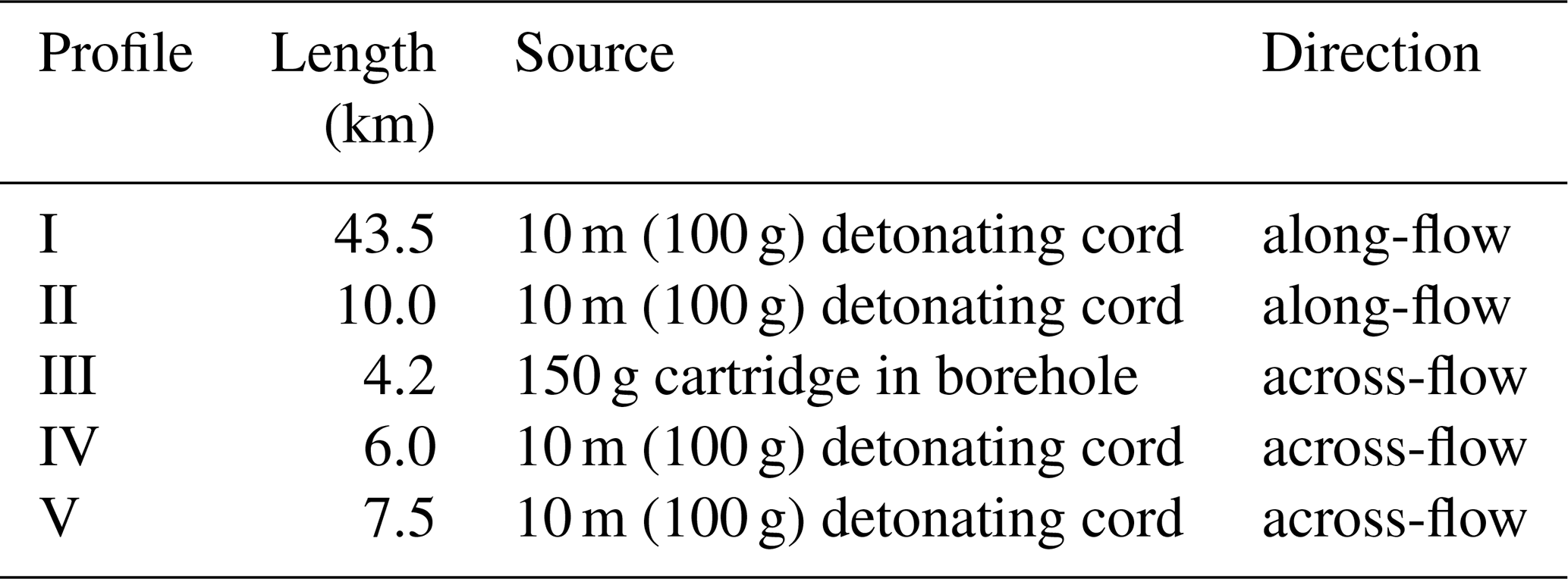
Early January 2017 we collected 71 km of seismic data divided over five profiles, numbered I to V (Fig. 1a, b). We used a 300 m snow streamer with 96 gimballed 30 Hz vertical compressional wave (P-wave) sensors, pulled behind a Nansen sledge carrying the recording equipment (four Geometrics GEODE units recording 24 channels each). The record length was set to 5 s and the sample interval to 0.5 ms. We used a snowmobile to pull the sledge and streamer between shot locations. As a source we mostly used 10 m detonating cord of 10 g m⁻¹ (so each shot used 100 g of PETN) placed 34 m in front of the near-offset geophone and parallel to the snow streamer. At profile III we used 5 m deep drilled boreholes filled with 150 g pentolite cartridges. The shot spacing was half a streamer length, 150 m, resulting in single-fold data coverage. We refer to the single-fold data as profiles (Table 1).

Table 1 Properties of the collected seismic profiles of SFG.

During the data acquisition we collected 13 long-offset gathers. At these shot locations we placed four shots of detonating cord at one location and recorded the shots at continuously decreasing offsets:

• Shot 1, offset 934 to 1234 m, streamer 934 m from the shot;

• Shot 2, offset 634 to 934 m, streamer 634 m from the shot;

• Shot 3, offset 334 to 634 m, streamer 334 m from the shot;

• Shot 4, offset 34 to 334 m, streamer 34 m from the shot, profiling configuration.

We used Shot 4 both in the long-offset gather and in profiling. We created three types of processed data sets for the following applications.

• Profiles. Here the processing aim is to get an x–z image (x axis is horizontal and z axis is vertical) revealing the dimension and structure of the ice, ocean cavity and seabed. The data were band-pass filtered (30–540 Hz), stacked, Kirchhoff time migrated and depth converted. In particular depth conversion of the time-migrated profiles is important as the basal channel area has considerable topography over a relative flat seabed. As the seawater is a slow P-wave velocity layer, thickness variation in the water column induces time delays in the underlying seabed and an apparent seabed topography in the time-migrated profiles.

• Single-shot gathers to determine the seismic reflection coefficient R. Here the aim is to map the amplitude values of different subsurface reflections and of the direct wave of raw shot gathers. Except for adding a geometry, these shots were not adversely processed as any processing affects the amplitudes.

• Long-offset gathers. Here we combine four shots with sequentially increasing offset into one shot location with a long offset. The aim here is to register the normal moveout (NMO) of a reflection for long offsets (time delay of a reflection with increasing offset) from which subsurface seismic P-wave velocities can be derived. The data were processed such that the reflections are best visible. Processing steps include muting, spiking deconvolution, band-pass and fk filtering.

2.6 Seismic reflection and transmission coefficient at normal incidence

Reflectivity at a planar and specular interface of two media in the subsurface depends on contrast of P-wave velocity (V_p), shear wave (S-wave) velocity (V_s), density (ρ) and the angle of incidence (θ) at the interface of the two considered media (Aki and Richards, 2002). At normal incidence the reflection coefficient R is solely determined by the contrast of the acoustic impedance (Z=ρV_p) at the media interface:

$$\begin{array}{}\text{(2)}& R={\displaystyle \frac{Z_{\mathrm{2}}-Z_{\mathrm{1}}}{Z_{\mathrm{2}}+Z_{\mathrm{1}}}}={\displaystyle \frac{{\mathit{\rho }}_{\mathrm{2}}{V}_{{\mathrm{p}}_{\mathrm{2}}}-{\mathit{\rho }}_{\mathrm{1}}{V}_{{\mathrm{p}}_{\mathrm{1}}}}{{\mathit{\rho }}_{\mathrm{2}}{V}_{{\mathrm{p}}_{\mathrm{2}}}+{\mathit{\rho }}_{\mathrm{1}}{V}_{{\mathrm{p}}_{\mathrm{1}}}}},\end{array}$$

where subscripts 1 and 2 refer to upper and lower media. The θ dependency of the reflection coefficient, R(θ), at a media interface can be expressed by

$$\begin{array}{}\text{(3)}& R\left(\mathit{\theta }\right)={\displaystyle \frac{A_{\mathrm{1}}\left(\mathit{\theta }\right)}{D{A}_{\mathrm{0}}}}r\left(\mathit{\theta }\right)e^{\mathit{\alpha }r\left(\mathit{\theta }\right)},\end{array}$$

with A₁(θ) being the amplitude of the primary reflection of the considered interface and A₀ being the source amplitude. D is a directivity factor caused by the use of detonating cord as a source (when using point sources such as borehole shots D=1), and r(θ) is the distance of the primary wave and α the seismic attenuation coefficient. These quantities can all be determined from single-shot records. The directivity factor D is discussed in Sect. 2.8.

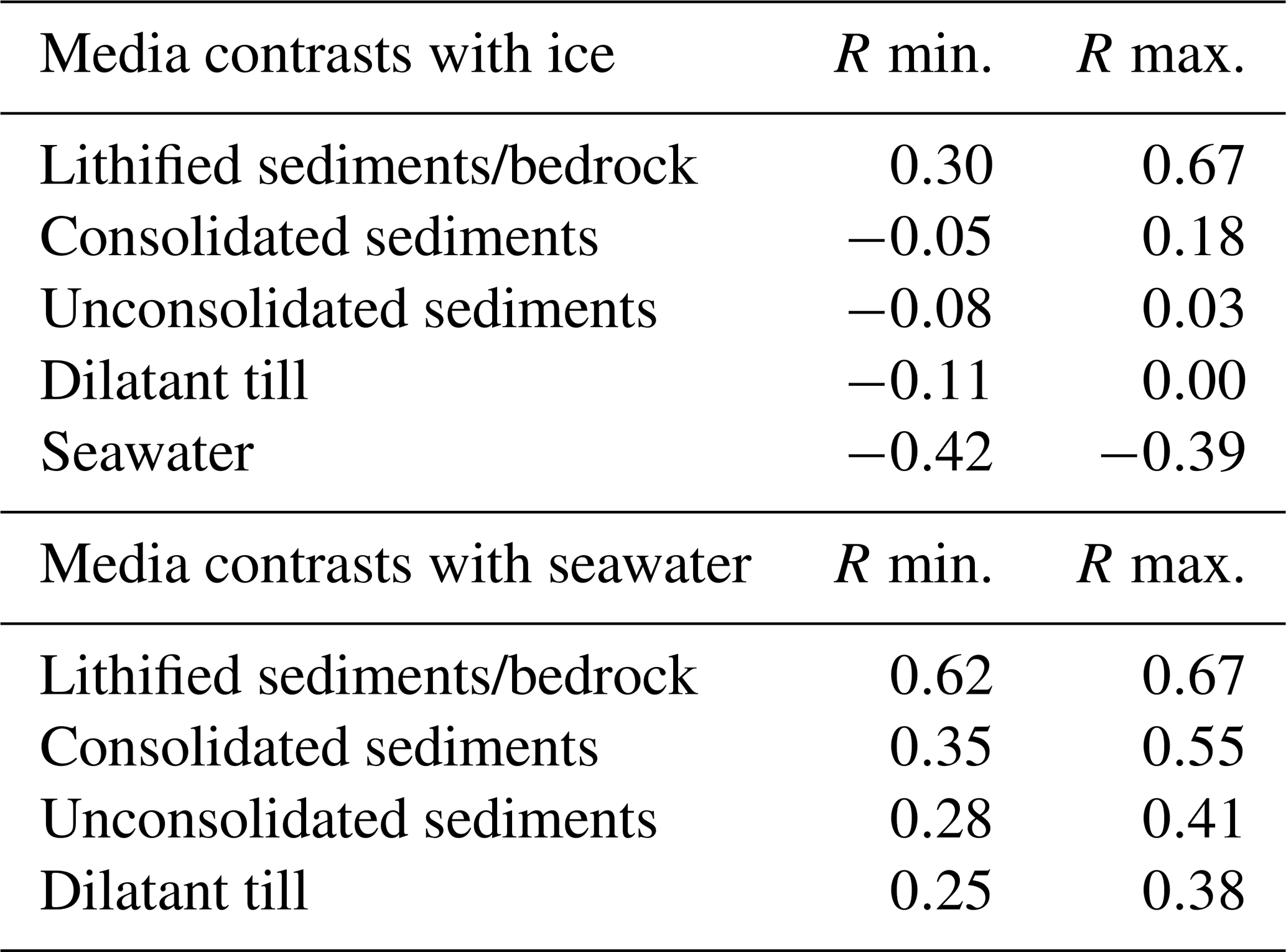
With a target depth of 1400 m or deeper, and an offset ranging from 33 to 330 m ($\mathrm{0.6}{}^{\circ }\le \mathit{\theta }\le \mathrm{6.7}{}^{\circ }$), the reflections of the profiling shots are considered as being normal incidence. A shortcoming of using a relative small spread is that we are not able to plot the θ dependency and perform an amplitude-versus-angle (AVA) analysis of subglacial or seabed materials, making identification less certain. Using the same values and lithology as Christianson et al. (2014), we calculated R at normal incidence (Table 2) from the following media interfaces we encounter in our survey area:

• grounded ice–bed interface,

• shelf ice–seawater interface,

• seawater–seabed interface.

In all cases of considered media interfaces, the acoustic impedance of the upper medium, ice (grounded or shelf ice) or the sub-shelf seawater can be estimated quite accurately as the material (ice or seawater) is known and the acoustic impedance of the lower medium (subglacial material or seabed) is unknown. Using both equations we can determine the acoustic impedance of subglacial material and the seabed from single shots.

Table 2 Ranges of R for different media contrasts at normal incidence. Top: if the upper medium Z₁ is ice. Bottom: if the upper medium Z₁ is seawater. The acoustic impedances and lithologies of the lower media Z₂ are similar to those in Christianson et al. (2014).

To calculate R at the seawater–seabed interface (R_s–b, where subscripts i, s and b refer respectively to ice, seawater and bed (both the bed upstream of the GL and seabed), respectively), we assume normal incidence. The smallest possible value for R is caused by an ice–seawater transition; with $Z_{\mathrm{i}}=\mathrm{3.44}\times {\mathrm{10}}^{\mathrm{6}}$ and $Z_{\mathrm{s}}=\mathrm{1.45}\times {\mathrm{10}}^{\mathrm{6}}$ $\mathrm{kg}{\mathrm{m}}^{-\mathrm{2}}{\mathrm{s}}^{-\mathrm{1}}$ we get

$$\begin{array}{}\text{(4)}& R_{\text{i–s}}={\displaystyle \frac{Z_{\mathrm{s}}-Z_{\mathrm{i}}}{Z_{\mathrm{s}}+Z_{\mathrm{i}}}}={\displaystyle \frac{(\mathrm{1.45}-\mathrm{3.44})\times {\mathrm{10}}^{\mathrm{6}}}{(\mathrm{1.45}+\mathrm{3.44})\times {\mathrm{10}}^{\mathrm{6}}}}=-\mathrm{0.41}.\end{array}$$

The transmission coefficient T is given by

$$\begin{array}{}\text{(5)}& T={\displaystyle \frac{\mathrm{2}{Z}_{\mathrm{1}}}{Z_{\mathrm{2}}+Z_{\mathrm{1}}}}={\displaystyle \frac{\mathrm{2}{\mathit{\rho }}_{\mathrm{1}}{V}_{{\mathrm{p}}_{\mathrm{1}}}}{{\mathit{\rho }}_{\mathrm{2}}{V}_{{\mathrm{p}}_{\mathrm{2}}}+{\mathit{\rho }}_{\mathrm{1}}{V}_{{\mathrm{p}}_{\mathrm{1}}}}}.\end{array}$$

To calculate R_s–b, we must take into account the energy loss at the ice shelf–seawater interface. To compensate for this energy loss, we assume normal incidence and an abrupt transition at the ice–seawater interface. Under these assumptions and with the ice–seawater transmission coefficient (T_i–s=1.41) and seawater–ice transmission coefficient (T_s–i=0.59), we get

$$\begin{array}{}\text{(6)}& R_{\text{s–b}}={\displaystyle \frac{A_{\mathrm{1}}\left(\mathit{\theta }\right)}{T_{\text{i–s}}{T}_{\text{s–i}}{A}_{\mathrm{0}}}}r\left(\mathit{\theta }\right)e^{\mathit{\alpha }r\left(\mathit{\theta }\right)}={\displaystyle \frac{A_{\mathrm{1}}\left(\mathit{\theta }\right)}{\mathrm{0.83}{A}_{\mathrm{0}}}}r\left(\mathit{\theta }\right)e^{\mathit{\alpha }r\left(\mathit{\theta }\right)},\end{array}$$

with A₁(θ) being the amplitude of the seabed reflection.

2.7 Seismic attenuation of the ice and seawater

To determine the seismic attenuation α, we need an estimate of the temperature of the shelf ice. We used temperature data from the 862 m long borehole FSW2 at the Filchner Ice Shelf at 80.56532^∘ S, 44.22546^∘ W, about 190 km downstream (northwest) of our survey area and another 275 km upstream from the calving front of the Filchner Ice Shelf. The installed thermistor chain showed an ice temperature range between −29 ^∘C at 10 m depth and −24 ^∘C at 650 m depth and then increasing to −2.3 ^∘C at the base. As the ice shelf at the survey area is thicker (1300 m), we extrapolated the temperature curve. Using this temperature profile, a centre frequency of 100 Hz, V_p=3750 m s⁻¹ we calculated average seismic attenuation of 0.2 km⁻¹ for the entire ice column (Peters et al., 2012; Bentley and Kohnen, 1976).

We used the seawater temperature from the same borehole data, −2.3 ^∘C, to calculate the seismic attenuation of the water column. Assuming a constant temperature for the entire subglacial seawater column, we get an attenuation of 0.001 dB km⁻¹ (Ainslie and McColm, 1998). This converts to $\mathrm{1.15}\times {\mathrm{10}}^{-\mathrm{4}}$ km⁻¹, which is so low that we can ignore this component.

With α of the ice and sea column known and Eqs. (6) and (3), we can calculate R. In general, one can say that the higher the water content of the lower medium Z₂, the smaller R (Table 2), but a distinction between unconsolidated sediments or dilated till is not possible. If ice is the upper medium, the range of R is larger than if the seawater is the upper medium, making the interpretation of the seabed more sensitive to uncertainties.

2.8 Determination of the source amplitude A₀

To determine A₀, we used the direct path method (Holland and Anandakrishnan, 2009), whereby the amplitudes of primary reflections of geophone pairs with a travel path ratio of 2 are compared. It was not possible to employ the alternative multiple bounce method (Smith, 1997), as the first multiple is hardly visible in the data. Assuming α does not change over the travel path, A₀ can be calculated. As our geophones are vertically orientated and the direct wave is a diving wave (a continuously refracted wave due to the continuous densification of the firn pack; Schlegel et al., 2019), we used pairs of traces at larger offsets (97 m and larger) from the source, which causes the ray path of the diving wave to arrive at angles closer to normal incidence.

The 10 m long detonating cord, placed in front of and parallel to the streamer, makes the source directional. Detonation creates a wave front spreading cylindrically, perpendicular to the detonating cord orientation and semi-spherical at the ends of the cord. The cylindrically spreading wave front contains more energy and mostly agitates the subsurface, whereas the spherically spreading wave front passes the streamer as a diving wave. This means we underestimate the source amplitude A₀ when using the direct path method.

At the ice–seawater interface, where the transition was abrupt, we determined A₀ by setting $R_{\text{i–s}}=-\mathrm{0.41}$. At these transitions we know the acoustic impedance of the upper and lower media, namely ice and seawater, so here we can calibrate R_i–s. We refer to these shots as calibrated shots. Transitions from shelf ice to the seawater are not always acoustically abrupt; accreted ice or placelet ice may have formed at the base of the ice, giving (most often) larger values for R_i–s and T_i–sT_s–i. We considered 26 shots (21 at profile I, 1 at profile III, 2 at profile IV and 2 at profile V) of which eight (six at profile I, one at profile IV and one at profile V) had an abrupt ice–seawater transition at the ∼9 m scale of vertical resolution. From these eight shots we derived the source amplitude A₀ reliably by setting $R_{\text{i–s}}=-\mathrm{0.41}$ and compared this with A₀ derived from the direct path method. The direct path method underestimates A₀ by a factor of 2.6, equivalent to the directivity factor D ($\mathrm{2.1}\le D\le \mathrm{3.1}$) from the cylindrically spreading source. To compensate for the directivity of the source amplitude, we use DA₀ as the directionally compensated source amplitude as shown in Eq. (3). The directionally compensated source amplitude has thus 19 % uncertainty.

Using DA₀ at five shots resulted in $R_{\text{i–s}}<-\mathrm{0.41}$. As we assumed $R_{\text{i–s}}=-\mathrm{0.41}$ is the smallest possible value for R, we set $R_{\text{i–s}}=-\mathrm{0.41}$ at these shots and also refer to these as calibrated shots. With these additional calibrated shots, we have a total of 13 calibrated shots (10 at profile I, 2 at profile IV and 1 at profile V) of the considered 26 shots.

Based on the noise level preceding the primary reflection of the bed or seabed, we determined A₁ with 7 % uncertainty. This means we determined R_s–b of the calibrated shots with 7 % uncertainty. Of the remaining 13 uncalibrated shots, where the directionally compensated source amplitude DA₀ has 19 % uncertainty, R_i–b and R_s–b could be determined with 32 % uncertainty.

3 Results and seismic interpretation

3.1 Seabed depth conversion

In the following we will present time-migrated and depth-converted profiles. Time-migrated sections are not suitable to unravel the subglacial stratigraphy of the seabed when the ice shelf thickness shows significant variability over short distances. This is the case around the basal channel where the base of the ice shelf has significant topography, and the underlying water column varies in thickness if the seabed is flat. As the seawater is a low-velocity layer (V_p=1425 m s⁻¹) in comparison to ice (V_p=3750 m s⁻¹), the thickness variation in the ice shelf causes significant time variation in the seabed returns. The time-migrated profiles show an apparent topography (an almost mirrored version of the topography of the base of the ice shelf) in the seabed caused by the different time delays of the ice shelf thickness. To improve the representation of the subsurface structure, it is thus important to convert the time-migrated seismic profiles to depth. In general this works quite well, but especially below the steep flanks of the basal channel the seawater–seabed morphology and seabed topography can not be properly recovered. The apparent morphology and topography of the seabed are influenced by the topography of the ice shelf.

3.2 Seismic profile I

The first 3.9 km of the 43.5 km long profile I (Fig. 2a) is grounded ice. The GL is at shot point (SP) 26 where the polarity of the ice base reflection reverses. There are 10 locations where $R_{\text{i–s}}=-\mathrm{0.41}$ and the shots are calibrated (Fig. 2b), 6 where the ice–seawater transition was abrupt and we calibrated $R_{\text{i–s}}=-\mathrm{0.41}$, and 4 locations, SP 208, 209, 231 and 273, where $R_{\text{i–s}}<-\mathrm{0.41}$ and was set $R_{\text{i–s}}=-\mathrm{0.41}$. Based on the topography, structure and the reflectivity of the ice-base contact and seabed contact, we distinguish four intervals in profile I.

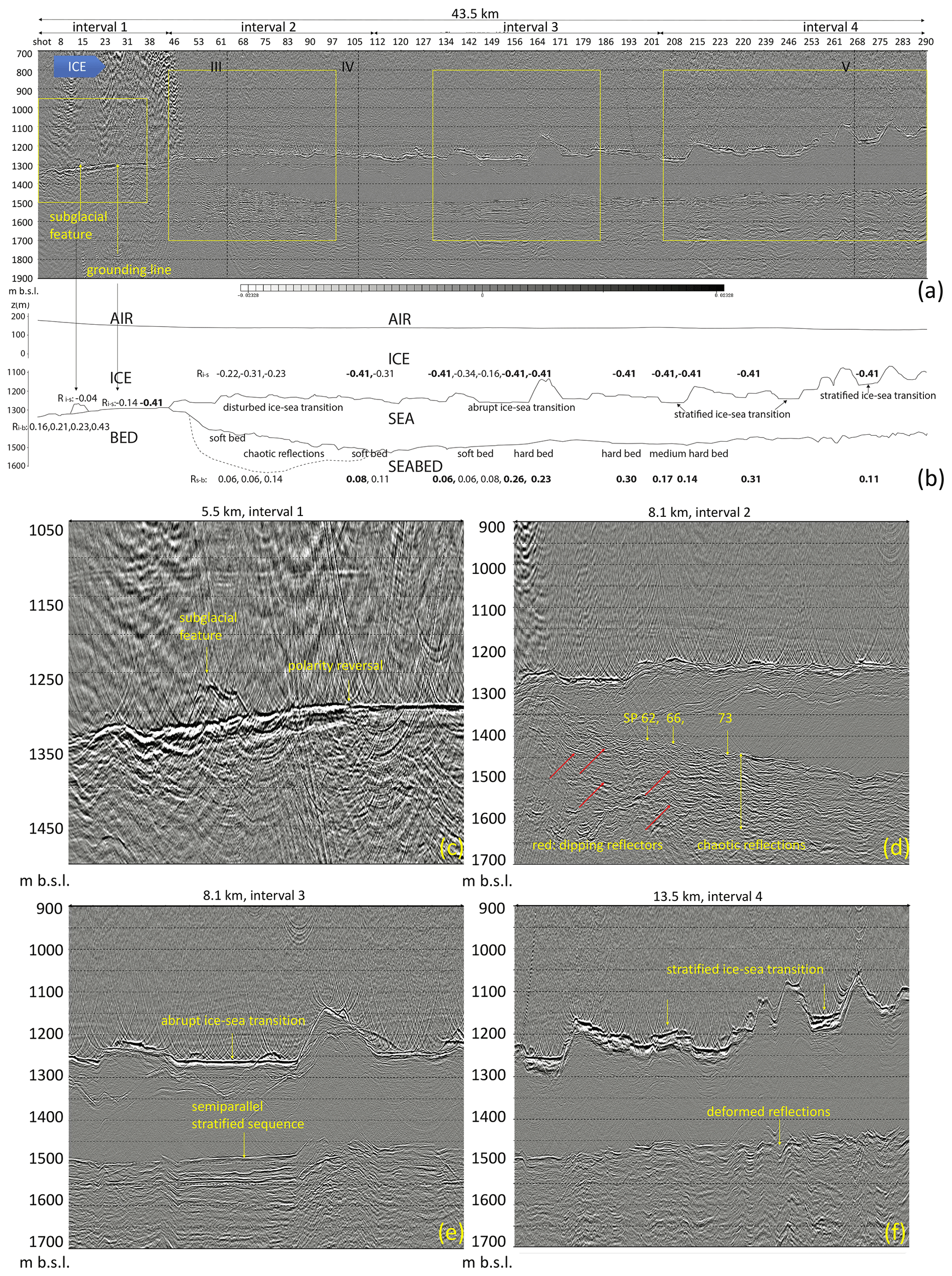
Figure 2 Profile I, its schematic diagram and four zooms showing the discussed characteristics. (a) Time-migrated and depth-converted seismic profile I. The ice flow is from left to right. Shot point (SP) numbering is along the x axis, increasing in the shooting direction. The profile is divided into four intervals marked by the double-headed arrows above the profile. The yellow frames represent four zooms shown in figures (c–f). The crossings of profiles III, IV and V are marked by the black dashed lines. (b) A schematic diagram of profile I marking the boundaries of the ice surface, base and the seabed. The calculated reflection coefficients R are shown at their position. The bold numbers represent calibrated shots and the normal numbers uncalibrated shots. (c) Zoom of interval showing the polarity reversal of the base at SP 26 and the subglacial feature at the flat bed. (d) The ∼200 m thick sedimentary sequence with chaotic reflections of the seabed marked by the dashed line in (b). Seaward-dipping reflections are marked by the red arrows. Reversed polarities are marked by the yellow arrows. (e) The ice–sea transition is abrupt, and the seabed consists of a harder, semi-parallel stratified sequence with fewer high-amplitude reflections. (f) The ice–sea transition has more concave cavities causing deformed reflections (apparent morphology) of the seabed.

Interval 1 is from SP 1 to SP 44 (Fig. 2a and c). We see a flat bed in direct or close contact with overlying ice. The bed starts at 1350 m b.s.l. at SP 1, rising to 1300 m b.s.l. at SP 26 after which the bed stays at 1300 m b.s.l. to SP 44. The polarity of the ice–bed contact of the grounded ice, which we refer to as positive in this paper, reverses (becomes negative) after SP 26 and stays like that for the rest of the profile. The location of the polarity change is within 150 m of the GL derived by interferometry (Fig. 1c). From SP 4 to SP 22 R_i–b increases from 0.16 to 0.43. From SP 26 to SP 44, R_i–s is negative and decreases from −0.14 at SP 30 to −0.41 at SP 33. The ice is floating but the thickness of the seawater column is too small to be made out.

At the base of the grounded ice, between SP 11 and SP 17, there is an elongated feature that appears to lie on a harder flat bed. It is approximately 50 m high and 1200 m long and $R=-\mathrm{0.04}$ at the ice bed contact. Our subsequent analysis shows this feature likely has evidence of a subglacial drainage channel and hereafter will be referred to as the subglacial feature.

Interval 2 is from SP 44 to SP 110 (Fig. 2a and d). The ice–seawater contact, the base of the ice shelf, lies between 1220 to 1300 m b.s.l., has minor topography with concave cavities 20 to 50 m above the surrounding base, and has R_i–s values varying between $-\mathrm{0.41}\le R_{\text{i–s}}\le -\mathrm{0.22}$. The ice–seawater contact is not abrupt, as the transition appears as an approximately 20 m sequence with chaotic reflections. This gradual ice–seawater transition probably leads to an increased energy loss and subsequently a larger (so less negative) R. At SP 44 the ocean cavity thickens as the seabed starts descending steeply with a slope of 4.1^∘ to 1400 m b.s.l. at SP 55 and then dips more gently with a slope of 1.1^∘ to 1500 m b.s.l. at SP 110. The polarity of the seabed contact is initially small and positive but occasionally, at SP 62, 66 and 73, negative. Between SP 51 and SP 95 the seabed consists of a ∼6.75 km long and ∼200 m thick sequence with chaotic to weakly stratified reflections. The reflections are mostly curved upward and discontinuous (100 to 600 m long) but occasionally dipping in a seaward direction marked by the red arrows (Fig. 2d). The amplitudes are high and show little signal loss with increasing depth; however boundaries (lower and lateral) are not abrupt. We will refer to this sequence as the sedimentary sequence with chaotic reflections. R_s–b varies between $\mathrm{0.06}\le R_{\text{s–b}}\le \mathrm{0.14}$. Downstream of SP 95 the character of the seabed gradually changes to a stratified sequence having fewer semi-parallel, high amplitude, reflections.

Interval 3 lies between SP 110 and 204 (Fig. 2a and e). The ice–seawater contact lies mostly between 1230 and 1260 m b.s.l. and is (semi)horizontally terraced interchanged with concave cavities 50 to 150 m above the surrounding base, reaching 1140 m b.s.l. at SP 164. The ice–seawater contact is more abrupt, especially in the lower (semi)horizontal terraces (SP 145 to SP 160 and SP 171 to SP 180). The seabed consists of a stratified sequence having fewer semi-parallel, high-amplitude reflections, hereafter referred to as the stratified sequence with semi-parallel reflections, and an increasing acoustic hardness downstream from R=0.06 at SP 130 to R=0.3 at SP 191. This harder, stratified sequence with semi-parallel reflections can best be observed between SP 145 and SP 160.

Interval 4 lies downstream of SP 204 (Fig. 2a and f). The ice–seawater contact now rises from 1270 to 1100 m, is less terraced and has more concave cavities. The ice–seawater transition at the terraces is no longer abrupt but a 20 to 30 m stratified sequence of semi-parallel reflections. This is especially visible in the lower terraces (SP 204 to SP 212, SP 243 to SP 250 and SP 269 to SP 276). At this interval the ice–seawater transition has been set to $R=-\mathrm{0.41}$ (SP 273) because the calculated $R<-\mathrm{0.41}$. The concave cavities have a more abrupt ice–seawater transition. At the seabed R ($\mathrm{0.11}\le R\le \mathrm{0.31}$) is quite variable, larger than in the second interval (SP 44–110) but not consistently high as in the third interval (SP 110–204). Despite the seabed being migrated and depth converted, it (SP 250–291) shows apparent morphology: the deformed reflections are influenced by the concave cavities of the ice–seawater transition.

3.3 Seismic profiles III, IV and V

The basal channel on all three profiles (Fig. 3) is terraced, especially on the western side where the channel has a mid- and a high-level roof (Fig. 3b). On profiles III and IV, the lower level of the ice shelf base lies at 1330 m b.s.l., and the roof of the basal channel lies at 1050 m b.s.l. At profile V the character of the channel roof is more rounded, but the terraces can still be made out. The base lies at 1250 m b.s.l. and the high-level roof of the basal channel at 920 m b.s.l.

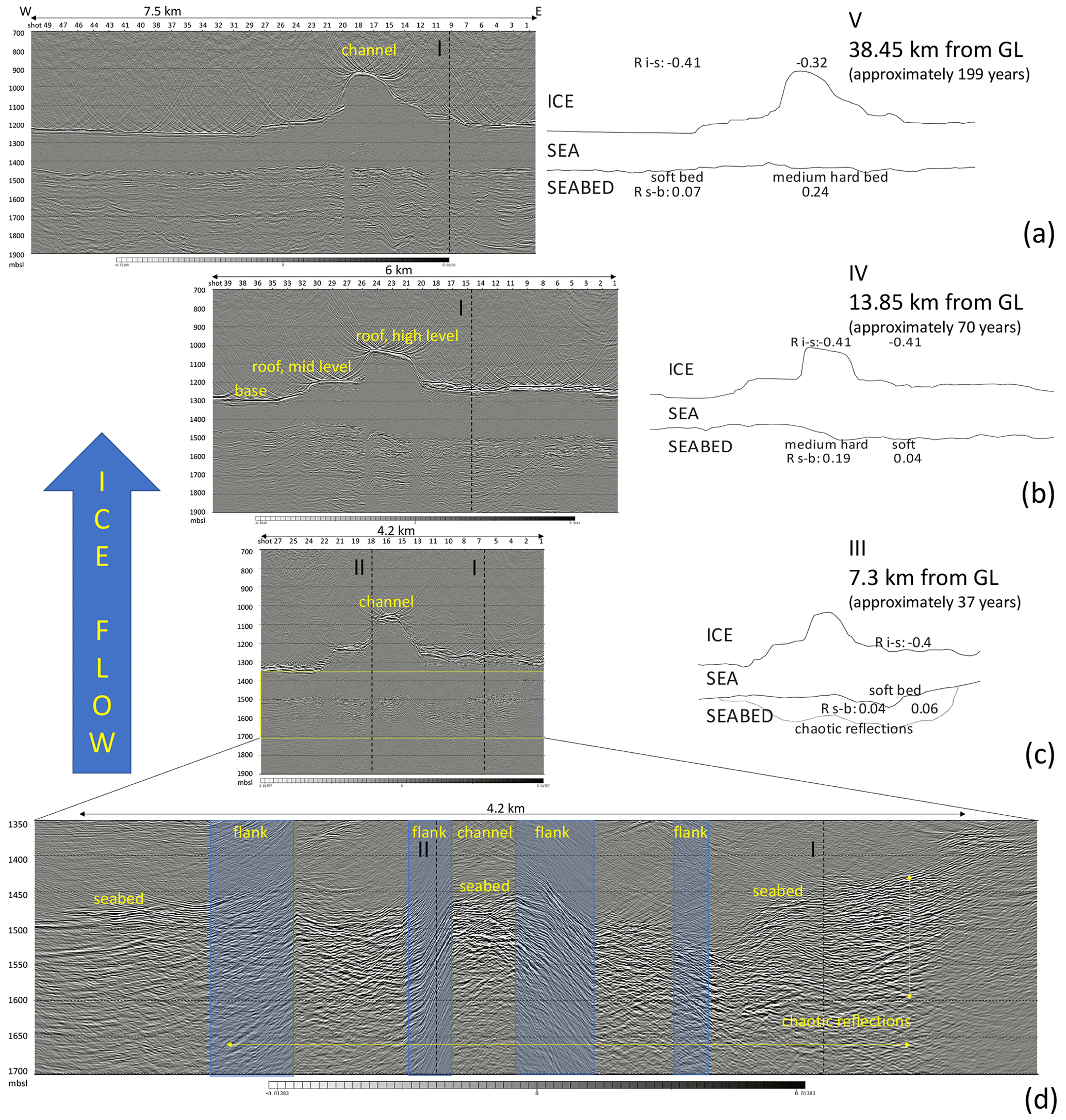
Figure 3 Profiles III, IV and V, their schematic diagrams showing the development of the basal channel, and a zoom of the seabed of profile III. The calculated reflection coefficients (bold represents calibrated shots) are shown at their position in the diagrams. The ice flow sequence is from bottom to top. The crossings of profiles I and II are marked by the black dashed lines. The distance from the GL and the time lap for the ice to reach this distance are mentioned on the right side. The three profiles have been aligned across-flow with respect to the most westerly flow line of Fig. 1a. (a) The most downstream profile V, with the high-level roof of the channel marked. (b) Profile IV, for clarity the high- and mid-level roofs of the channel as well as the base are marked. (c) The most upstream profile III. The yellow frame marks a zoom of the seabed shown in (d). The sedimentary sequence with chaotic reflections is marked in the schematic diagram by the dashed line. (d) The seabed of profile III showing the extent of the sedimentary sequence with chaotic reflections, also marked by the yellow arrows. The shaded rectangles mark the flanks of the basal channel where the depth conversion and morphology of the seabed break down.

The seabed at the profiles lies between 1450 and 1500 m b.s.l. (Fig. 3), but the migration and depth conversion (and thus the morphology) of the seabed under the steeper flanks of the basal channel are not correct. This is especially true for profile III, the shortest profile of the three, where the flanks are a significant part of the entire profile. Profiles IV and V have a flat seabed that only shows some apparent morphology under the steeper flanks of the basal channel. The western side of profile IV is 50 m higher than its eastern side. At profiles IV and V the seabed below the basal channel has R_s–b=0.19 and R_s–b=0.24.

At profile III (Fig. 3c) we used charges in 5 m deep boreholes, whereas profiles IV and V were recorded with detonating cord. The borehole charges produce a ghost with 5–7 ms delay, not present when using detonating cord at the surface. This causes the source wavelet of the borehole charges to be longer than that of the detonating cord. As a result, the ice–seawater and seawater–seabed contacts of profile III are not as well resolved (they appear more stratified) as for profiles IV and V.

Profile III crosses the sedimentary sequence with chaotic reflections of interval 2 (Fig. 3d). As both the topography of the basal channel and the ghost affect the topography and morphology of the seabed, we determined the extent of the sedimentary sequence solely by its increased amplitude. The sedimentary sequence is 3.2 km wide, centred under the basal channel and thinning from east to west. It is ∼150 m thick at the crossing with profile I (eastern side) and ∼100 m at the crossing with profile II (western side). The sedimentary sequence is absent on the outer eastern and western sides (start and end) of the profile. At SP 11 the sedimentary sequence has R_s–b=0.04, and at SP 7, the crossing with profile I, R_s–b=0.06.

3.4 Profile II

Profile II, crossing the sedimentary structure with chaotic reflections of profile III, has a complex structure as it unintentionally was recorded over the western flank of the basal channel. This resulted in two ice–sea reflections, one from the roof and one from the base of the basal channel, making interpretation difficult. However the seabed below the basal channel can clearly be made out (Fig. 4a). The 6 km long profile of the seabed, between SP 67 and 28, shows the sedimentary sequence extends over a length of 2.85 km from SP 59 to 41. The sedimentary sequence forms a topographic high at the seabed; its surface dips seaward with a 1.3^∘ slope and possibly overlays bedrock. The sedimentary sequence fills two cavities, a smaller cavity between SP 59 and 54, reaching a thickness of ∼50 m, and a larger cavity between SP 54 and 40, reaching a thickness of ∼100 m at the crossing with profile III. The sedimentary sequence has clearer stratification than in profile I but, likewise, has seaward-dipping reflections. The reflections have more continuity (up to 1500 m long) but are still somewhat chaotic.

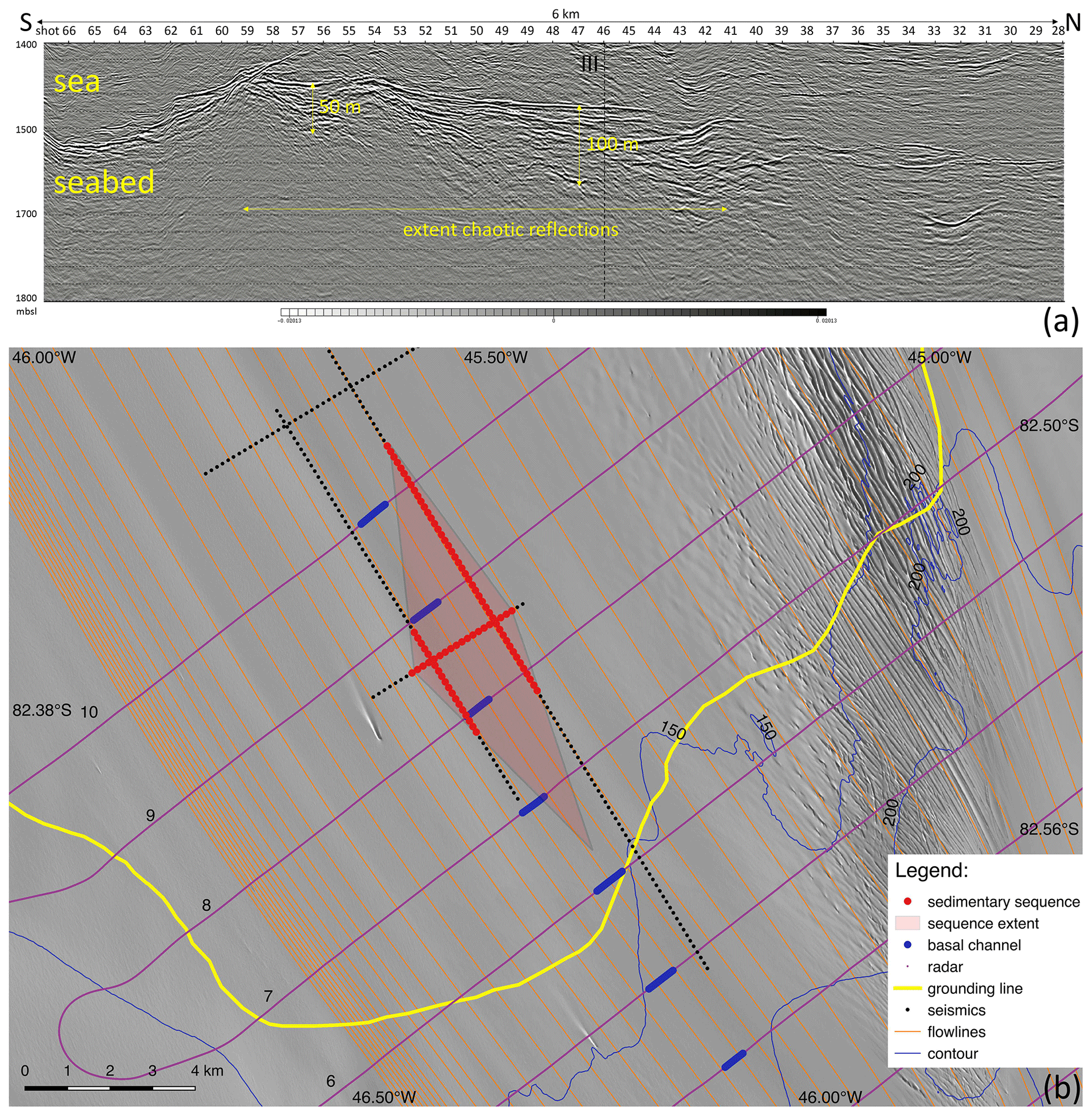
Figure 4 The extent of the sedimentary sequence with chaotic reflections at profile II (a) and its lateral extent over profiles I, II and III (b). (a) The seabed of profile II with the ice flow from left to right. The sedimentary sequence is marked by the yellow double-headed arrows, the horizontal arrow marking the lateral extent and the two vertical arrows marking the thicknesses at two cavities. The crossing with profile III is marked by the black dashed line. (b) The seismic (black and red dots) and radar survey (purple looping lines) of the GL area showing the seismic shots (red dots) that recorded the sedimentary sequence with chaotic reflections on profiles I, II and III. The red shaded area marks the outer boundaries of the sedimentary sequence by using linear interpolation. The grounding line is marked in yellow. The basal and subglacial channels are marked by the blue dots. The background is a shaded version of the 8 m Reference Elevation Model of Antarctica (REMA; Howat et al., 2019).

The sedimentary sequence with chaotic reflections is present on profiles I, II and III. To detect the extent of the sedimentary sequence, we plotted the seismic shots showing the sedimentary sequence (Fig. 4b, red dots) and linearly extrapolated its outer boundaries. This is represented by the red shaded area. Towards the GL these extrapolated lines represent a first-order estimate of the lateral boundaries of the sedimentary sequence and point to the origin of deposition. The lateral boundaries cross each other 750 m downstream of the subglacial channel entrance into the ocean cavity (blue dots in profile 6; profiles with numerals refer to Fig. 5).

3.5 Radar images of basal channel

We selected 10 airborne radar profiles separated by 2.6 km in the along-flow direction (Fig. 5) tracking the basal and, upstream of the GL, the subglacial channel (the feature between the ice and bed upstream of the basal channel, probably water filled). They are ∼3.75 km long, and their numbering corresponds to Fig. 1d. The radar profiles are rotated 5^∘ anticlockwise with respect to the seismic across-flow profiles. Profile 10 is 10.9 km downstream of the GL, profile 6 is at the GL (partly grounded and partly at shelf) and profile 1 is 12.8 km upstream of the GL.

Figure 5 Return power, grey-scaled and depth-converted radar profiles 1 to 10. Figure 1d shows their position. The ice flow direction is from bottom to top, starting with profile 1 (upstream) at the lower right corner up to 10 (downstream) in the upper left corner. The semi-automatically picked basal reflection (seawater and bed) of the ice is marked in blue. At profiles 1 to 5 the ice is grounded, profile 6 is at the grounding line and at profiles 7 to 10 the ice is floating.

In Fig. 6 we combine the basal reflection of the ice of the 10 migrated radar and the three seismic profiles in a schematic diagram to track the development of the subglacial and basal channel along its flow line. All 3.75 km long profiles have been lined up against the westernmost flow line of Fig. 1a. The resolution of the radar data is not as good as that of the seismic data, so the shape of the basal channel can not be reconstructed as well; nevertheless, we can track it. On the grounded ice we can track the subglacial channel at profiles 3, 4, 5 and 6 where it increases in size from hardly distinguishable from the surrounding bed to a height of 280 m at profile 6 at the grounding line and continues as a basal channel under the ice shelf. The basal channel meanders up to profile 9 after which the three remaining profiles 10, IV and V show a consistent westward migration. The height of the subglacial and basal channel is hard to determine accurately, partly because of the poorer resolution of the radar profiles but also because it is hard to determine what the base of the ice shelf exactly is, so the heights should be seen as an indication rather than an exact measurement. In general the height of the basal channel is ∼175 m between profiles 7 and IV and then increases to 205 m.

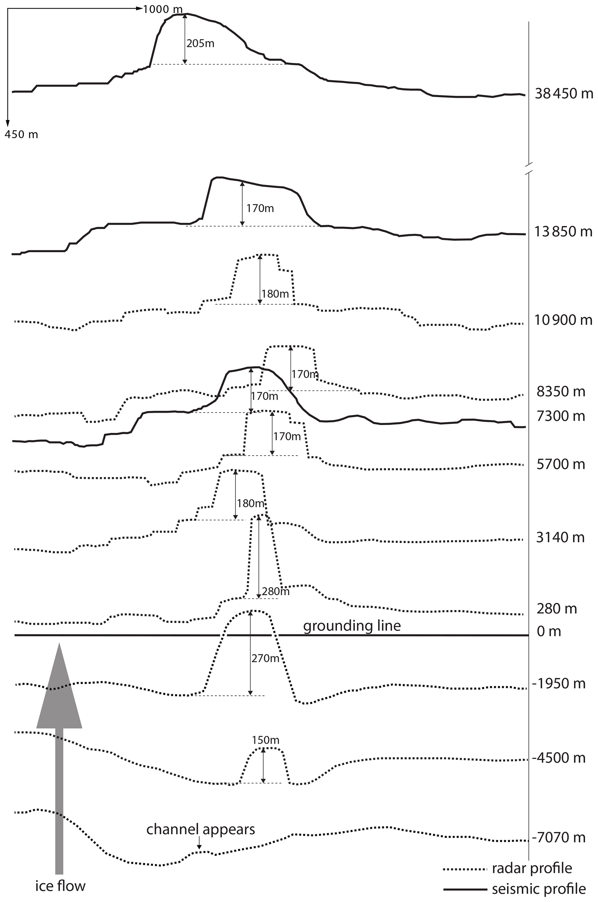
Figure 6 A schematic diagram of the shape and development of the subglacial channel under the grounded ice and basal channel under the ice shelf. The scheme combines the migrated radar (dashed) and seismic (continuous) profiles that are vertically exaggerated. The vertical axis shows the distances to the grounding line measured along the westerly flow line of Fig. 1d.

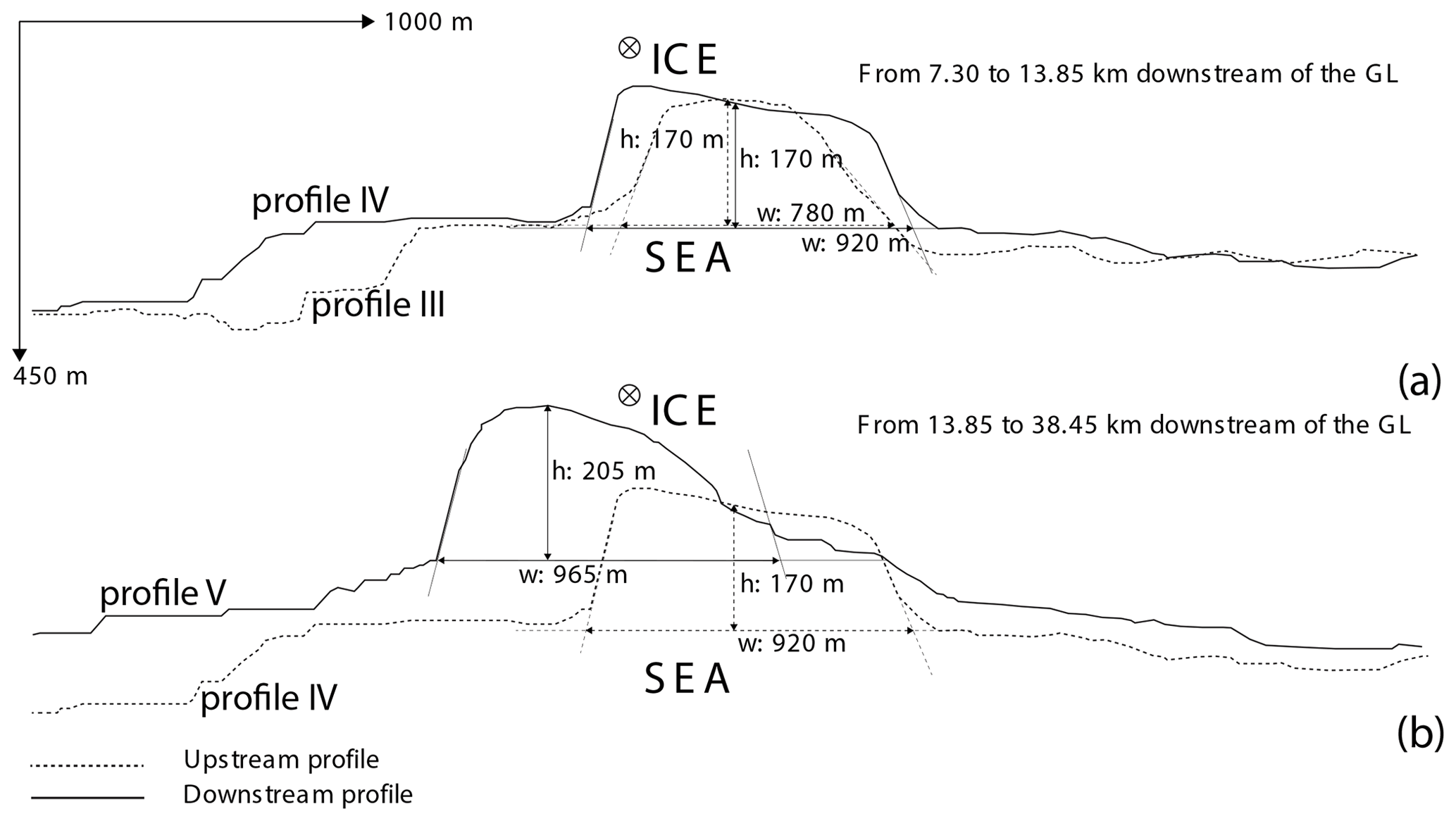
Figure 7 A schematic diagram of the ice shelf development around the basal channel derived from the three seismic across-flow profiles in Fig. 3. Vertically, they are positioned with respect to the ice shelf surface so that the ice thickness can be compared. (a) Comparing profile III (dashed line) with IV (continuous line). (b) Comparing profile IV (dashed line) with V (continuous line).

To see the changing geometry of the basal channel, we restrict ourselves to the migrated, depth-converted seismic profiles that reproduce the shape of the basal channel more accurately than the radar profiles (Fig. 7). From profiles III to IV (Fig. 7a), the terraced, multi-levelled roof of the channel stays preserved but widens from some 780 to 920 m, whereas the ice shelf thickness, surrounding the channel, stays almost constant. The flanks of the basal channel become steeper but the height does not change noticeably, although there may be some lowering in the centre of the basal channel. From profiles IV to V (Fig. 7b), the terraced basal channel becomes less pronounced and the base is shallower (i.e. the ice shelf thins). As a result profile V moved upward. The basal channel also moved westward with respect to profile IV, so in a downstream direction. The flat roof of the channel becomes more rounded and the lower level roof on the western side less pronounced.

4 Discussion

4.1 The grounding line position

At profile I the polarity of the basal reflection reverses at SP 26 from positive to permanently negative in the downstream direction (Fig. 2a). As negative polarity indicates the presence of water at the base, this suggests the ice uncouples from the bed. Between SP 30 and 33 we see a decrease from $R_{\text{i–s}}=-\mathrm{0.14}$ to $R_{\text{i–s}}=-\mathrm{0.41}$, which is probably caused by an increase in water content in the subglacial bed. At SP 33 the ice is in contact with the seawater. We recorded SP 26 at 17:06 UTC, 1 January 2017. According to five GPS stations 13 km downstream from the GL, this is 3.5 h after high tide at which time there was 1.5 m additional uplift on a tidal range of 2.6 m. As SP 26 lies within 150 m of the GL derived from interferometry, we refer to the GL as the one provided by interferometry in the remainder of the paper.

4.2 The structure of the ice shelf and ocean cavity

Looking at the structure of the ice sheet at the GL area of profile I (Fig. 2), we see an almost constant ice thickness gradient when the ice, initially flowing over a flat bed, passes the GL. Unlike the classic picture of the sheet–shelf transition, where rapid ice shelf thinning close to the GL causes a steeply rising ice shelf base, the sheet–shelf transition of SFG seems to be a mirrored version of this: SFG has a steeply descending seabed at SP 44 and an almost constant ice thickness gradient downstream of the GL. This steeply descending seabed, the onset of the ocean cavity, probably determines the GL position. The absence of an ocean cavity at the flat ice shelf base upstream of SP 44 confirms this.

Generally we would expect the highest melt rates at the deepest part of the ice shelf, the GL, as that is where the melting point is lowest due to the pressure effect of the ocean. The topographically constrained ice flow, confirmed by the parallel flow lines (Fig. 1a) and the flat ice shelf base, allow us to use the ice thickness gradient as a first-order approximation for basal melt (Fig. 2). As the base of the ice shelf is initially flat, any topography in the base is likely to be caused by basal melt. The constant ice thickness gradient of the ice passing the GL suggests there is little basal melting at the GL of SFG.

Once in contact with the ocean cavity at SP 44, there is some basal melting as the base of the ice shelf has some topography, but this increases in the downstream direction as we see an increase in the number and the magnitude of concave cavities in the ice base. Interval 2 has some topography but small compared to intervals 3 and 4. Interval 3 has one pronounced concave cavity at SP 164 interchanged with lower terraces, and interval 4 has several pronounced concave cavities, at SP 215 and downstream of SP 250, interchanged with lower terraces. Dutrieux et al. (2014) observed a similar ice shelf geometry and attributed the terrace-shaped structure to a steplike thermohaline ocean structure causing organized melting.

That there is little melting at the GL increasing in the downstream direction is also confirmed by the seismic profiles of Fig. 7b. The ice shelf thickness of profiles III and IV does not change much in depth, but the basal channel itself widens. At Pine Island Glacier this channel widening was ascribed to ice dynamics, i.e. convergence at ice shelf surface and divergence at ice shelf base (Dutrieux et al., 2013; Vaughan et al., 2012). At SFG we observed no noticeable ice convergence at the surface channel, at least not distinguishable from the noise level. As such we attribute this initial basal channel widening to melting along the flanks caused by upward-moving seawater. This vertical motion (and thus melting along flanks) of seawater is possible because of the basal topography of the channel. For the same reason we see an increase in size of the ocean cavities in the downstream direction. Between profiles IV and V we observe a general thinning of the ice shelf, both above the basal channel and outside of it. Profile V crosses profile I in interval 4 where there is increased basal melting of the ice shelf.

4.3 Properties of the seabed

At profile I we recorded 10 calibrated and 11 uncalibrated shots. At the calibrated shots we will use R, having 7 % uncertainty, for interpretation. At the uncalibrated shots where R has 32 % uncertainty, we use the trend of the magnitude and polarity of R for interpretation rather than the actual value.

At all the places where the ice–seawater contrast is not abrupt, the propagating P-wave, travelling from the ice shelf into the seawater, encounters a series of transmissions and reflections rather than a single transmission. The total amplitude loss over such a stratified ice–seawater contrast is probably larger than our assumed transition of Eq. (6). At these places we most likely underestimate R_s–b.

While still grounded, we see an increase in R_i–b from 0.16 to 0.41 over a 3.9 km distance. As we find it less likely that the subglacial material changes drastically over this short along-flow interval and as the acoustic impedance Z of the ice is constant, we attribute this steady increase in acoustic impedance of the subglacial material to increasing compaction, as has been observed by Christianson et al. (2013). We interpret the bed of the grounded ice thus as subglacial till.

Once the ice passed the GL at SP 26, the floating ice stays close to its flat base down to SP 44 when the seabed starts to descend steeply. The seabed downstream of SP 44 consists of two distinguishable environments. At interval 2, close to the GL, we have a 6.75 km long, 3.2 km wide and 200 m thick sedimentary sequence with chaotic reflections that changes into a stratified sequence with semi-parallel reflections at intervals 3 and 4. The sedimentary sequence with chaotic reflections close to the GL, having smaller values for R_s–b, consists of softer, more porous material then the stratified sequence with semi-parallel reflections. The softness is confirmed by the occasionally negative polarity at the steeper downslope of the seabed. We interpret the sequence as an unconsolidated sedimentary sequence.

The stratified sequence with semi-parallel reflections generally has higher values for R_s–b, indicating a harder material. This is particularly clear in interval 3, where $\mathrm{0.23}\le R_{\text{s–b}}\le \mathrm{0.30}$. The seabed structure representative for this second type of environment is most clearly visible between SP 146 and 161, where the flat featureless and abrupt ice–sea contact does not influence the seabed morphology. In interval 4 we calculated lower values for R_s–b, but these low values all have a stratified ice–seawater contact above them, and so the amplitude loss at the ice–sea transition may be larger than is accounted for and probably underestimates R_s–b. Based on R_s–b≈0.31, we interpret them as consolidated sediments but can not exclude bedrock. In any case, this part of the seabed has properties of an eroded surface, where softer deposits are missing. It could have been created during periods of higher ice-dynamic activity, e.g. during one or several advances of SFG during the last glacial into Last Glacial Maximum (LGM) positions of maximum advance.

4.4 Characteristics of the subglacial feature

At profile I, below the grounded ice between SP 11 and 17, we see the subglacial feature. If this seismic event is from the nadir, it would be a separate, 1200 m long and approximately 50 m high subglacial feature on a hard bed, its dimensions represented by the red semi-circle in Fig. 8. The reflection coefficient $R_{\text{i–b}}=-\mathrm{0.04}$ represents an ice-unconsolidated, water-saturated sediment contact, so most likely the subglacial feature would be a subglacial conduit on a hard flat bed. A 50 m high conduit would show up in the radar profiles 5 and 6, crossing profile I just upstream and downstream of the subglacial feature, but both profiles show a flat base at nadir. We also do not see any evidence of any other subglacial channel entering the ocean cavity on the western side of SFG.

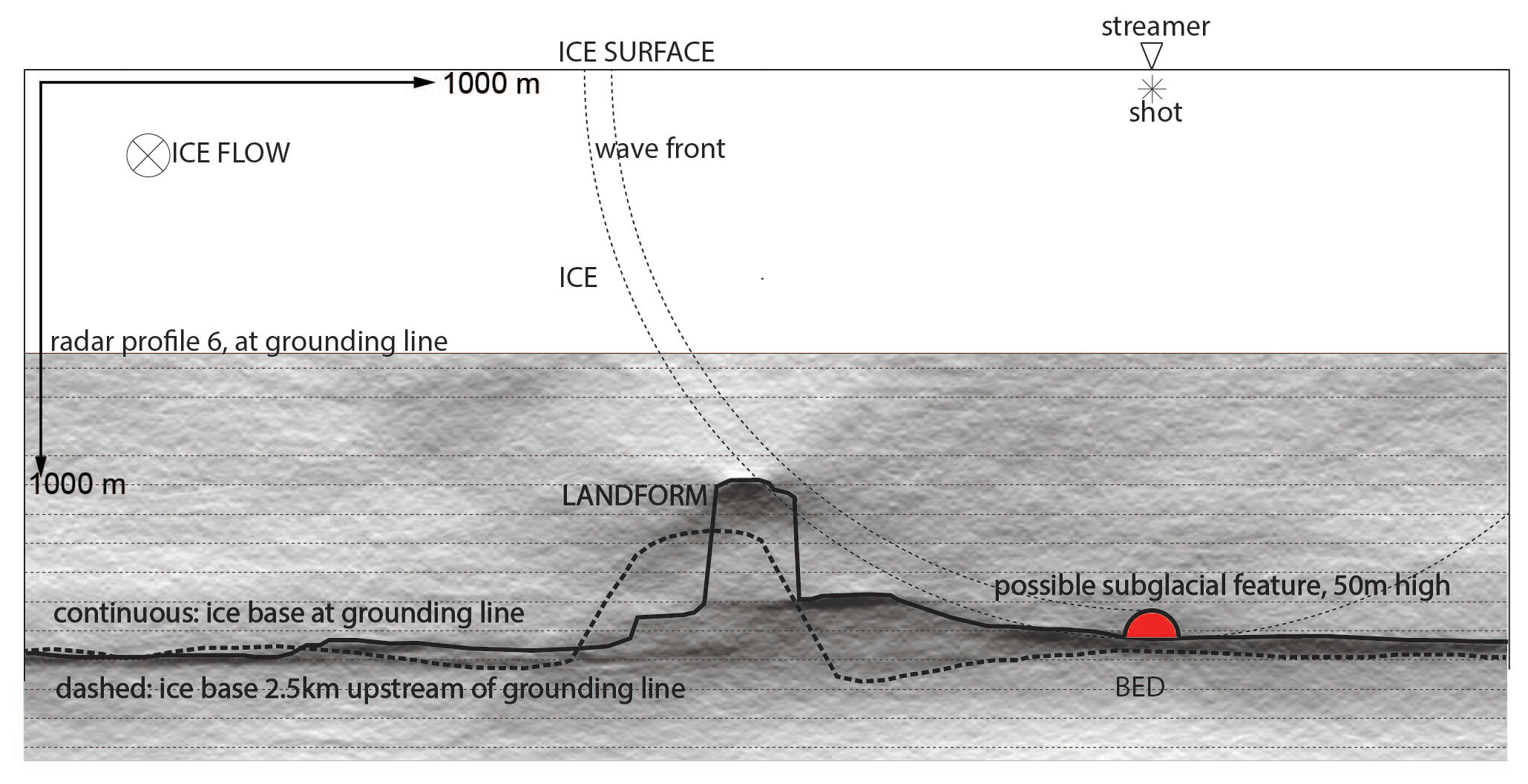
Figure 8 Cross section of the seismic recording geometry of profile I during SP 11 to 17 when the subglacial feature was recorded. The shooting and ice-flow direction are into the page, perpendicular to the cross section. The continuous and dashed black lines represent the ice base at the GL (continuous, profile 6) and 2 km upstream (dashed, profile 5) from the GL. The subglacial feature can either be at nadir, in which case its dimensions are represented by the red semi-circle, or the feature can be off-nadir, in which case the feature likely represents the top of the subglacial channel from profile 6. The spherical wave front (dashed quarter circle) shows the off-nadir reflections from the top the basal channel (profile 6) arrive just before the nadir flat bed reflections (so when no semi-circle would be present).

A more likely interpretation is that the subglacial feature is from off-nadir and represents the top of the subglacial channel connecting to the basal channel (Fig. 6). The spherically spreading wave front arrives at the subglacial channel off-nadir before it reaches the bed at nadir (Fig. 8). When the subglacial channel reaches the dimension of profile 6, this is probably the case. We interpret the subglacial feature as the top of the ∼280 m high subglacial channel approaching the GL.

4.5 The subglacial hydrological interpretation

Our subglacial drainage model predicts a significant (190×10³ m³ a⁻¹) freshwater influx on the western side of the ice shelf of SFG (Fig. 1b). At the grounded ice of SFG, profiles 3, 4, 5 and 6 show a subglacial channel connecting to the basal channel at the grounding line. Over a length of 7 km approaching the GL, the subglacial channel increases its size from hardly distinguishable from the bed to a 280 m height at the grounding line. The increase in size, when approaching the grounding line, is likely caused by the ocean interacting with the subglacial channel due to tidal motion, thereby melting the channel walls, as suggested by Drews et al. (2017) and Horgan et al. (2013) and modelled by Walker et al. (2013). Once past the grounding line, this wide opening of the subglacial channel adjusts to hydrostatic equilibrium and forms the basal and surface channel in which the subglacial drainage water incises. This setting is similar to the subglacial estuary described by Horgan et al. (2013). Because the subglacial channel connects to the only basal channel at the western side of the ice shelf, and because we have a large subglacial drainage influx modelled at the western side of the ice shelf, we interpret the subglacial channel to be a subglacial drainage channel.

The grounded part of profile I consists of a sediment layer and, judging by its reflectivity, becomes more consolidated closer to the grounding line. So the subglacial drainage channel probably travels over a layer of subglacial sediments with varying consolidation. We do not know the exact nature of the subglacial drainage system, but the radar and seismic profiles do suggest channelized flow close to the grounding line. We are possibly dealing with a channel that, upstream and outside the survey area, is coupled to a surrounding distributed system as described by Hewitt (2011). Close to the grounding line channelized flow is favourable, which corresponds to our observations.

Profiles I, II and III show a 6.75 km long, 3.2 km wide and ∼200 m thick sedimentary sequence with chaotic to weakly stratified reflections that occasionally dip seaward, just downstream of the GL. The lateral boundaries of this sedimentary sequence, estimated by linear interpolation, converge towards the subglacial drainage channel at the GL. This makes the subglacial drainage channel the likely source of deposition and explains the seaward-dipping reflections of this sedimentary sequence. As the sedimentary sequence is fan shaped and point sourced, we interpret it as a grounding line fan (Powell, 1990) or an ice-proximal fan (Batchelor and Dowdeswell, 2015). We assume the centre of deposition is where the sedimentation is thickest at profile I, which is somewhat east of the basal channel. This may be caused by the direction of the subglacial drainage channel, which is, when approaching the GL slightly more eastward than the ice flow direction (Figs. 1d and 4b, radar profiles 5 and 6). The sedimentary sequence consists of unconsolidated, probably subglacial terrestrial sediments with an estimated volume of ∼1.13 km³ (half the volume of a 6.75 km high ellipsoid cone with two semi-axes of 1.6 and 0.2 km). The seabed between SP 60 and 90 dips with 1.1^∘. These dimensions are large but not unusual for grounding line fans (Dowdeswell et al., 2015), and SFG is a major ice stream. The ocean cavity with a steeply descending seabed facilitates the development of a large grounding line fan by sediments transported through the subglacial drainage channel and deposited by gravity flows. This explains the chaotic reflections and the seaward-dipping reflections in this sedimentary sequence. Similar fans have been found at the Hudson Bay area as remnants of the Laurentide Ice Sheet (Lajeunesse and Allard, 2002).

What is unusual here is that the fan has formed under the ice shelf of SFG in a region without surface melt, which is a common characteristic of fans (Powell and Alley, 1997). But we do have evidence for channelized flow at the grounding line, a noble gas sample observation suggesting a freshwater influx of terrestrial origin likely (Huhn et al., 2018) and a significant modelled channelized freshwater influx on the western side of SFG confirmed by the presence of a single basal channel on the western side. We also have an unusual ocean cavity with a steeply descending seabed and a stable grounding line and a fan-shaped sedimentary sequence most likely deposited by a subglacial channel. These are typical conditions for the formation of a fan at the grounding line (Powell, 1990; Powell and Alley, 1997; Batchelor and Dowdeswell, 2015).

5 Conclusions

We investigated the characteristics of a subglacial channel continuing as a basal channel across the grounding line of the Support Force Glacier. As this is the only subglacial channel–basal channel system on the western side of Support Force Glacier, subglacial drainage takes place through channelized flow close to the grounding line. Our observations concur with the categorization of Alley et al. (2019), i.e. subglacially sourced channels that intersect the grounding line and coincide with modelled subglacial water drainage. We find no evidence for the hypothesis that the basal channel is initially formed by a landform as suggested by Jeofry et al. (2018b). The increase in channel height close to the grounding line is probably caused by the ocean interacting with the subglacial channel, thereby increasing its height as suggested by Horgan et al. (2013) and Walker et al. (2013).

In seismic profiles I, II and III at the seabed, close to the grounding line, we identify an 6.75 km long, 3.2 km wide and 200 m thick, fan-shaped sedimentary sequence with chaotic reflections. Towards the grounding line, the extrapolated outer boundaries of this sedimentary sequence converge to the subglacial drainage channel. This makes the subglacial drainage channel the likely source of deposition, and as such we interpret this sedimentary sequence as a grounding line fan, which is unusual for ice shelves and areas without surface melt.

Further downstream the seabed consists of harder, stratified consolidated sediments with semi-parallel reflections, possibly bedrock. We consider these two units to originate from different development phases: whereas the harder sequence is potentially a leftover from a farther advanced grounding line, e.g. coming along with stronger erosion during advances into the glacial, the softer sediment sequence seems to be the result of comparatively recent post-glacial and Holocene grounding line depositions.

Apart from the basal channel and individual concave cavities, the base of the ice shelf downstream of the grounding line is relatively flat, indicating that basal melt rates are relatively low. We attribute the observed widening of the basal channel to melting along its flanks, which we also observe at the flanks of concave cavities in the ice shelf base. The melting increases further in the downstream direction. To date it is unlikely that warmer water is already in the cavity near the grounding line. But even if it were, the geometry of the steeply descending seabed downstream of the grounding line would limit the direct contact of potentially warmer water with the ice shelf base, thus limiting basal melt rates, unless the cavity was fully flooded with warmer water. This is in contrast to the typically envisaged geometry and ice–ocean interaction at grounding lines, which often envisage a steeply rising ice shelf base just downstream of grounding lines, where circulation is dominated by the ice pump mechanism. With our improved characterization of the grounding line area of SFG, future modelling studies should investigate how differently this region might react to the presence of warm deep water in the cavity than for instance the glaciers in the Amundsen Sea Embayment region and thus quantify the role of the seabed geometry.