Geodetic point surface mass balances: a new approach to determine point surface mass balances on glaciers from remote sensing measurements

Mass balance observations are very useful to assess climate change in different regions of the world. As opposed to glacier-wide mass balances which are influenced by the dynamic response of each glacier, point mass balances provide a direct climatic signal that depends on surface accumulation and ablation only. Unfortunately, major efforts are required to conduct in situ measurements on glaciers. Here, we propose a new approach that determines point surface mass balances from remote sensing observations. We call this balance the geodetic point surface mass balance. From observations and modelling performed on the Argentière and Mer de Glace glaciers over the last decade, we show that the vertical ice flow velocity changes are small in areas of low bedrock slope. Therefore, assuming constant vertical velocities in time for such areas and provided that the vertical velocities have been measured for at least 1 year in the past, our method can be used to reconstruct annual point surface mass balances from surface elevations and horizontal velocities alone. We demonstrate that the annual point surface mass balances can be reconstructed with an accuracy of about 0.3 m of water equivalent per year (m w.e. a⁻¹) using the vertical velocities observed over the previous years and data from unmanned aerial vehicle images. Given the recent improvements of satellite sensors, it should be possible to apply this method to high-spatial-resolution satellite images as well.

1 Introduction

Glacier surface mass balance observations are widely used to assess climate change in various climatic regimes because of their sensitivity to climate variables (e.g. Zemp et al., 2019; Marzeion et al., 2014; Kaser et al., 2006; Gardner et al., 2013; Huss and Hock, 2018; IPCC, 2019). In situ surface mass balance measurements have been conducted on only a few of the 200 000 mountain glaciers worldwide (WGMS, 2017; Zemp et al., 2019). In the European Alps, about a dozen annual surface mass balance time series from in situ measurements extending over more than 50 years are available (WGMS, 2017). Recently, considerable efforts have been made to assess ice volume changes at the mountain-range scale over long time periods using geodetic measurements obtained from remote sensing techniques (e.g. Paul and Haeberli, 2008; Abermann et al., 2011; Gardelle et al., 2012; Gardner et al., 2013; Berthier et al., 2014; Brun et al., 2017). These geodetic methods determine glacier-wide volume changes, or glacier-wide mass balances, by differencing repeated determinations of glacier surface elevations obtained from airborne and spaceborne surveys usually over multi-year to decadal periods (e.g. Vincent, 2002; Bauder et al., 2007; Soruco et al., 2009; Berthier et al., 2014; Dussaillant et al., 2019). These methods are effective for estimating the overall glacier mass change and quantifying the related hydrological impacts or sea level contribution (e.g. Hock et al., 2005; Kaser et al., 2010; Huss, 2011; Immerzeel et al., 2013; Zemp et al., 2019). However, the meaningfulness of a climatic interpretation of these results is questionable. Indeed, glacier-wide mass balances are not solely driven by changes in climate but also by changes in glacier geometry controlled by the dynamic response of each glacier (Vincent, 2002; Fischer, 2010; Abermann et al., 2011; Huss et al., 2012; Vincent et al., 2017). Consequently, they do not provide a direct climatic signal. On the other hand, point surface mass balances provide a direct climatic signal which depends only on local ablation and accumulation (Huss and Bauder, 2009; Thibert et al., 2013; Vincent et al., 2004, 2017, 2018b). Ablation is related directly to the surface energy balance. Accumulation is related to precipitation but is also strongly influenced by valley topography. Indeed, glaciers are generally surrounded by very steep non-glacial slopes which capture precipitation over a larger area than that of the glacier itself. In this way, high accumulation values are due to downhill transportation and strong wind actions (Vincent, 2002). Statistical modelling enables us to extract a climatic signal from heterogeneous in situ observations of point mass balance networks independently of effects related to ice flow dynamics and glacier area changes (Vincent et al., 2018b). However, these previous studies showed that it is crucial to perform observations of annual point surface mass balance at the same locations every year. Unfortunately, the only way to presently obtain point mass balance data is to make in situ measurements. In particular, the net annual ablation in the ablation zone is usually obtained from ablation stakes. These point surface mass balance measurements require huge efforts involving field campaigns and the collection of data from stake measurements scattered over the glacier. This explains why so few in situ measurements are performed, especially on glaciers located in remote areas with very difficult access (e.g. Azam et al., 2018; Wagnon et al., 2013; Hoezle et al., 2017).

The objective of this paper is to propose an approach to determine point surface mass balances from measurements obtained by remote sensing techniques. In this way, we aim to determine point surface mass balances in ablation areas without setting up ablation stakes each year. We will develop this method using a comprehensive dataset of in situ measurements and analysis of ice motion, elevation changes and point surface mass balance data in the ablation area of the Argentière Glacier (French Alps). We will then validate our method in other areas of the ablation zone of this glacier and of the Mer de Glace glacier.

2 Study area

The Argentière Glacier is located in the Mont Blanc range, French Alps (45^∘55^′ N, 6^∘57^′ E). Its surface area was about 10.9 km² in 2018 (Fig. 1). The glacier extends from an altitude of about 3400 m a.s.l. (above sea level) at the upper bergschrund down to 1600 m a.s.l. at the snout. The length of this glacier is about 10 km. It faces north-west except for a large part of the accumulation area (south-west facing tributaries). The annual surface mass balance ranges roughly from 2 m of water equivalent per year (m w.e. a⁻¹) in the accumulation area to about −10 m w.e. a⁻¹ close to the snout. This glacier is free of rock debris except for the lowermost part of the tongue below the ice fall located between 2000 and 2300 m a.s.l. In the region studied in detail at 2350 m, the ice is generally free of debris. The debris cover can be 5 to 10 cm thick in some locations. The field observations of the Argentière Glacier (i.e. mass balance, thickness variations, ice-flow velocities and length fluctuations over 50 years) come from the French glacier monitoring programme called GLACIOCLIM (Les GLACIers, un Observatoire du CLIMat; https://glacioclim.osug.fr/, last access: 25 February 2021). For the present study, additional detailed observations were carried out in the framework of the SAUSSURE programme (Sliding of glAciers and sUbglacial water preSSURE; https://saussure.osug.fr, last access: 25 February 2021). The main part of our study focuses on a small area of the Argentière Glacier (∼0.2 km²) located between 2320 and 2400 m a.s.l. in the ablation zone (Figs. 1 and 2). In this area, the glacier is ∼ 600 m wide, the horizontal ice flow velocity is ∼ 55 m a⁻¹ (Vincent et al., 2009), and the maximum ice thickness is 250 m (Rabatel et al., 2018). Experiments conducted through boreholes (Hantz and Lliboutry, 1983) indicate that the bed is composed of hard rock with no thick or deforming sediment layer.

3 Data

In the selected area, annual point surface mass balances and ice flow velocities were monitored with a high positioning accuracy at the end of each ablation season between 2016 and 2019 from 19 ablation stakes (Fig. 2). Our study also used surface mass balance and ice flow velocity observations from a small part of the ablation zone of the Mer de Glace glacier at the location named “Tacul glacier” (Fig. 1).

The ablation stakes are 10 m long and made of five 2 m long sticks tied together with metallic chains. We performed the observations of annual point surface mass balance at the same locations every year. Errors in ablation measurements mainly come from the mechanical play of the jointed sticks. The uncertainties in the annual surface mass balance measurements performed in this ablation zone have been assessed at ±0.14 m w.e. a⁻¹ (Thibert et al., 2008). Topographic measurements were performed to obtain the 3D coordinates of the ablation stakes. For this purpose, we used a Leica 1200 Global Navigation Satellite System (GNSS) receiver, running with dual frequencies. Occupation times were typically 1 min with 1 s sampling, and the number of visible satellites (GPS and GLONASS) was more than seven. The distance between fixed and mobile receivers was less than 1 km. The Differential Global Positioning System (DGPS) positions have an intrinsic accuracy of ±0.01 m. However, given the size of the holes drilled to insert the stakes, we estimate that the stake positions have an uncertainty of ±0.05 m.

Both velocity components are required. The vertical velocity is the vertical component of the surface velocity obtained from measuring altitude differences of the bottom tip of stakes. For this purpose, the emergence measurement is required to obtain the buried length of the stake. Thus, the purpose of emergence observations is two-fold. They enable us (i) to calculate the surface mass balance from two field campaigns and (ii) to obtain the altitude of the bottom tip of the stake using the altitude of the surface. In practice, the DGPS measurements are performed simultaneously with the emergence measurements in order to obtain the exact position of the bottom tip of the stake buried in ice. In this way, it is possible to monitor ice velocity along the three coordinate directions. Depending on the tilt of the ablation stakes, the size of the drilling hole and the mechanical play of the jointed stakes, we assume that the annual horizontal and vertical velocities are known with an uncertainty of ±0.10 m a⁻¹.

Aerial photographs of the glacier surface were taken on 5 September 2018 and 13 September 2019 using the senseFly eBee X unmanned aerial vehicle (UAV). A total of 720 photos in 2018 and 673 photos in 2019 were collected with the on board senseFly S.O.D.A. camera (20 MP RGB sensor with a 28 mm focal length from an average altitude of 140 m above the glacier surface). Prior to the survey flights, we collected GNSS measurements of ground control points (GCPs) that consist of rectangular pieces of red fabric (100×60 cm) with white painted circles (40 cm diameter) on the glacier (10 in 2018, 20 in 2019) and ten 40 cm diameter white circles painted on rocks on the sides of the glacier. The original horizontal resolutions of the orthophoto mosaics and digital elevation models (DEMs) are 10 cm and 1.00 m, respectively. The photos from the survey were processed using the structure for motion (SfM) algorithm that is implemented in the Agisoft Metashape Professional version 1.5.2 software package (Agisoft, 2019). The SfM stereo technique was then used to generate a dense point cloud of the glacier surface. This dense point cloud was used to construct the DEMs using the GCPs surveyed during the field campaigns. A detailed description of the processing steps can be found in Kraaijenbrink et al. (2016) and Brun et al. (2016). The horizontal resolutions of the orthophoto mosaics and DEMs are 10 cm and 1.0 m, respectively.

To calculate horizontal ice flow velocities over the studied area, we used the UAV orthophoto mosaics with COSI-Corr (Co-registration of Optically Sensed Images and Correlation), a software tool developed for image correlation (Leprince et al., 2007; Ayoub et al., 2009). Due to the velocities of the Argentière Glacier in this region (∼ 55 m a⁻¹), we resampled the UAV orthophotos at 1.0 m resolution because the correlation was too noisy even with very large window sizes (i.e. 512 pixels). The surface velocities were computed using an initial window size of 256 pixels, a final window size of 64 pixels and a step of 4 pixels. The output velocity field was filtered using signal-to-noise ratios (SNRs) provided by COSI-Corr. Using an SNR threshold greater than 0.9 provides a good compromise between output details, noise and computing time. A detailed description of the correct choice of the window size for correlation can be found in Kraaijenbrink et al. (2016).

To establish the possible errors in the correlation process, horizontal displacements on stable off-glacier areas were evaluated over 25 random points and provided a maximum horizontal error of ∼ 0.55 m.

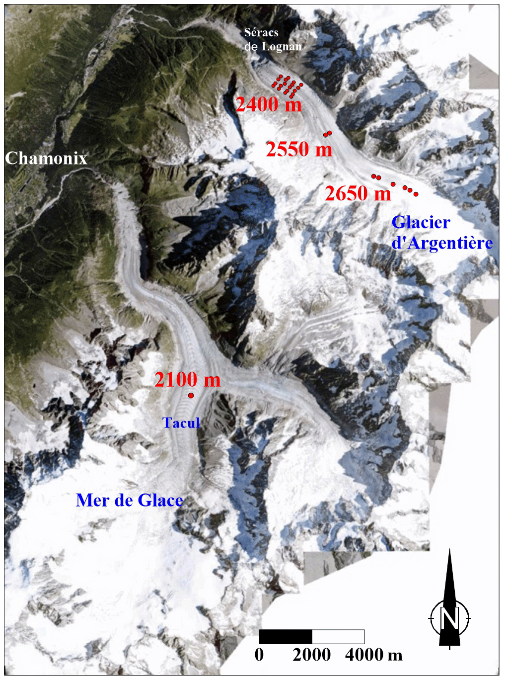
Figure 1 Map of the Argentière and Mer de Glace glaciers. The red dots on the Argentière Glacier are the ablation stakes used in this study for annual surface mass balance and ice flow velocity measurements in three regions of the glacier (at approximately 2400, 2550 and 2700 m a.s.l.). Aerial photo from the French National Geographical Institute, 2015 (https://www.geoportail.gouv.fr/, last access: 25 February 2021).

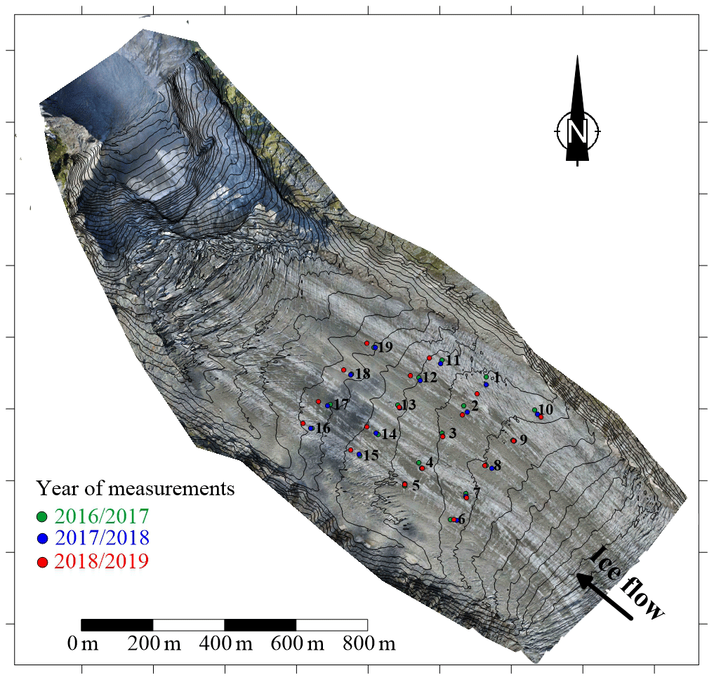
Figure 2 Map of the studied area in the ablation zone of the Argentière Glacier. The contour lines of surface topography correspond to the surface in 2018. The green, blue and red dots are the positions of the ablation stakes used for surface mass balance and ice flow velocity measurements when they were set up in 2016, 2017 and 2018, respectively. Aerial photo from unmanned aerial vehicle survey (5 September 2018).

4 Method

We will now introduce the mathematical framework used further on.

4.1 Emergence velocities

The emergence velocity is the upward or downward flow of ice relative to the glacier surface. This flow compensates for the surface mass balance exactly if the glacier is under steady state conditions. The surface elevation change equation (Cuffey and Paterson, 2010, p. 332) expresses the surface mass balance as a function of surface velocity and surface gradient:

$$\begin{array}{}\text{(1)}& b_{\mathrm{s}}=\partial S/\partial t-(w_{\mathrm{s}}-u_{\mathrm{s}}\partial S/\partial x-v_{\mathrm{s}}\partial S/\partial y),\end{array}$$

with b_s the surface mass balance expressed in metres of ice, firn or snow (m a⁻¹), S the surface elevation (m), u_s, v_s and w_s the components of ice flow velocity at the surface (m a⁻¹), $\partial S/\partial x$ the surface gradient in the x direction, and $\partial S/\partial y$ the surface gradient in the y direction.

The term $w_{\mathrm{s}}-u_{\mathrm{s}}\partial S/\partial x-v_{\mathrm{s}}\partial S/\partial y$ is called the emergence velocity. If the horizontal x axis is taken in the flow direction, v_s=0, and the emergence velocity is written as

$$\begin{array}{}\text{(2)}& v_{\mathrm{e}}=w_{\mathrm{s}}-u_{\mathrm{s}}\partial S/\partial x.\end{array}$$

Note that under steady state conditions, $\partial /\partial t=\mathrm{0}$ and $b_{\mathrm{s}}=-v_{\mathrm{e}}$. The emergence velocities can be calculated for each ablation stake from horizontal and vertical velocities and the slope of the surface $\partial S/\partial x$. In this way, we assume that the downslope direction is the flow direction. The slope of the surface can be obtained from GNSS field measurements and calculated over a distance similar to that travelled by the stake over 1 year. In the ablation zone, the emergence velocities are positive, which corresponds to an upward flow of ice relative to the glacier surface. Note also that the vertical velocity can be positive or negative in any region of the glacier. The emergence velocity is a classical way to relate the surface mass balance to the thickness changes (Eq. 1). Unfortunately, as shown later in our study (Sect. 6.1), even if the horizontal and vertical velocities are accurately measured, the large uncertainties related to the slope and thickness changes prevent us from calculating the point surface mass balance from the emergence velocities.

At the yearly scale, according to Eq. (1) and Fig. 3 and considering that the x axis is taken along the flow line direction (i.e. v_s=0), the annual surface mass balance B_s between the years t and t+1 is obtained from

$$\begin{array}{}\text{(3)}& B_{\mathrm{s}}=\mathrm{\Delta }{h}_{\mathrm{1}}+U_{\mathrm{s}}\tan {\mathit{\alpha }}_{t+\mathrm{1}}-W_{\mathrm{s}}=\mathrm{\Delta }{h}_{\mathrm{2}}+U_{\mathrm{s}}\tan {\mathit{\alpha }}_t-W_{\mathrm{s}},\end{array}$$

where $u_{\mathrm{s}}\cdot \partial S/\partial x$ is replaced by U_s tanα_t or U_s tan α_t+1, U_s is the annual surface horizontal velocity, and tanα_t and tan α_t+1 are the slopes for the years t and t+1, respectively. W_s is the annual vertical velocity. $\partial S/\partial t$ is replaced by Δh₁ and Δh₂, which are the annual thickness changes observed at the ends of the annual ice flow vectors.

Figure 3 illustrates the components of Eq. (3).

Note that the slope of the surface may change from year t to year t+1 and the expression depends on the selected slope and thickness changes Δh₁ or Δh₂ (Fig. 3). Obviously, the results are the same.

Figure 3 Diagram illustrating horizontal, vertical and emergence velocities (m a⁻¹) observed from an ablation stake (orange). U_s (m a⁻¹) and W_s (m a⁻¹) are the components of horizontal and vertical velocities, α_t and α_t+1 are the slopes for the years t and t+1, respectively, Z_s1,t and $Z_{\mathrm{s}\mathrm{2},t+\mathrm{1}}$ are the elevations of the surface at each end of the ice flow vector, and Δh₁ and Δh₂ are the elevation changes (m) at each end of the ice flow vector.

4.2 Calculation of the geodetic point surface mass balance

Let us reconsider the emergence velocity formulation in order to express the point surface mass balance as a function of vertical velocity and altitude changes at the ends of the annual displacement vector.

According to Eq. (3) and given that $\mathrm{\Delta }{h}_{\mathrm{1}}+U_{\mathrm{s}}\tan {\mathit{\alpha }}_{t+\mathrm{1}}=\mathrm{\Delta }{h}_{\mathrm{2}}+U_{\mathrm{s}}\tan {\mathit{\alpha }}_t=Z_{\mathrm{s}\mathrm{2},t+\mathrm{1}}-Z_{\mathrm{s}\mathrm{1},t}$ (Fig. 3), we can write the following:

$$\begin{array}{}\text{(4)}& B_{\mathrm{s}}=Z_{\mathrm{s}\mathrm{2},t+\mathrm{1}}-Z_{\mathrm{s}\mathrm{1},t}-W_{\mathrm{s}}.\end{array}$$

This expression has a great advantage in that it does not depend on the surface slope that can change from one year to the next. It is also independent of thickness changes that can change from one site to another.

The term geodetic point surface mass balance refers to the value of B_s obtained from Eq. (4). Once the vertical velocity is known, B_s can be obtained from topographical surface measurements alone. Note that even if the horizontal velocity is not included in Eq. (4), it is needed to estimate the positions at which $Z_{\mathrm{s}\mathrm{2},t+\mathrm{1}}$ and Z_s1,t should be measured.

5 Results

5.1 Annual horizontal and vertical velocities over the 3 years

Annual horizontal and vertical velocities were measured from a network of 19 ablation stakes over 3 years between 2016 and 2019 (Fig. 2). The stakes were replaced each year and were always set up at the same locations using a handheld GPS device, allowing a relevant comparison, except for stakes 1 and 11 which were located in areas with large crevasses, preventing the possibility of drilling stakes at the chosen location. In addition, for the year 2018/2019, stake 12 was accidentally replaced at a distance of more than 30 m from its initial position due to both a lack of rigour and the uncertainty in the handheld GPS measurement. This difference in locations led to a difference in the horizontal velocity of 3 m a⁻¹ in a region with a strong horizontal gradient (left edge of the area in Fig. 4). However, it does not change the pattern of horizontal velocities or horizontal velocity changes with time. This is not the case for vertical velocities as described in the next paragraph. In the area of this network, the annual horizontal velocities range from 35 to 60 m a⁻¹. The annual ice flow velocities have been interpolated from kriging over the entire coloured areas shown in Fig. 4. In this way, we can accurately compare the ice flow velocities over 3 years, 2016/2017, 2017/2018 and 2018/2019, at the locations of each stake (Fig. 5a). Strong deceleration in horizontal ice flow velocities can be observed over these 3 years. On average, ice flow velocity decreased by 2.4 and 1.8 m a⁻¹ over the two periods 2016/2017–2017/2018 and 2017/2018–2018/2019, which corresponds to an average decrease of about 4.8 % and 3.6 % per year, respectively. Note that the regression lines shown in Fig. 5a are almost parallel, which means that the change in velocities is homogeneous in space.

The vertical velocities were obtained from the altitude changes in the bottom tip of the stakes from one year to the next (Fig. 3). In the studied area, the vertical velocities can be positive or negative and range from −4 to 4 m a⁻¹ (Fig. 4). The vertical velocities have been interpolated over the entire coloured areas shown in Fig. 4 using kriging. The patterns of vertical velocities are very similar for the years 2016/2017 and 2017/2018. We note some differences with the 2018/2019 pattern. As mentioned previously, stakes 1, 11 and 12 set up in 2018/2019 are located at distances of more than 30 m from their initial positions. In addition, stakes 17, 18 and 19 were replaced in 2018 at distances ranging between 25 and 30 m from their initial positions. These six stakes are shown with small dots in Fig. 5b. If we exclude the velocity values of 2018/2019 for these stakes, we can conclude that the measured vertical velocities are very similar over this 3-year period. The differences do not exceed 0.5 m a⁻¹. The average of the differences is 0.01 m a⁻¹, and the standard deviation is 0.29 m a⁻¹. These differences barely exceed the measurement uncertainty. Note also that the vertical velocity changes could be affected by the horizontal motion changes or vertical strain rate changes as discussed in Sect. 6.

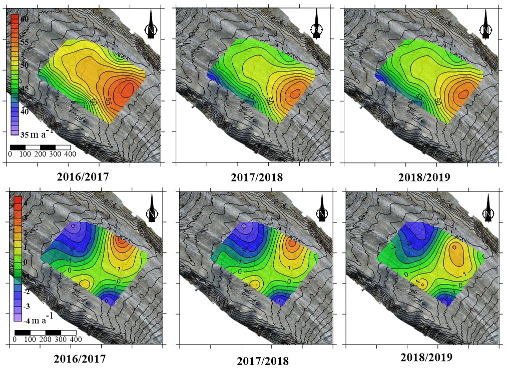
Figure 4 Horizontal (top panels) and vertical (bottom panels) ice flow velocities (m a⁻¹) measured over 3 years from the ablation stakes. Note the different colour scales. Distances in metres.

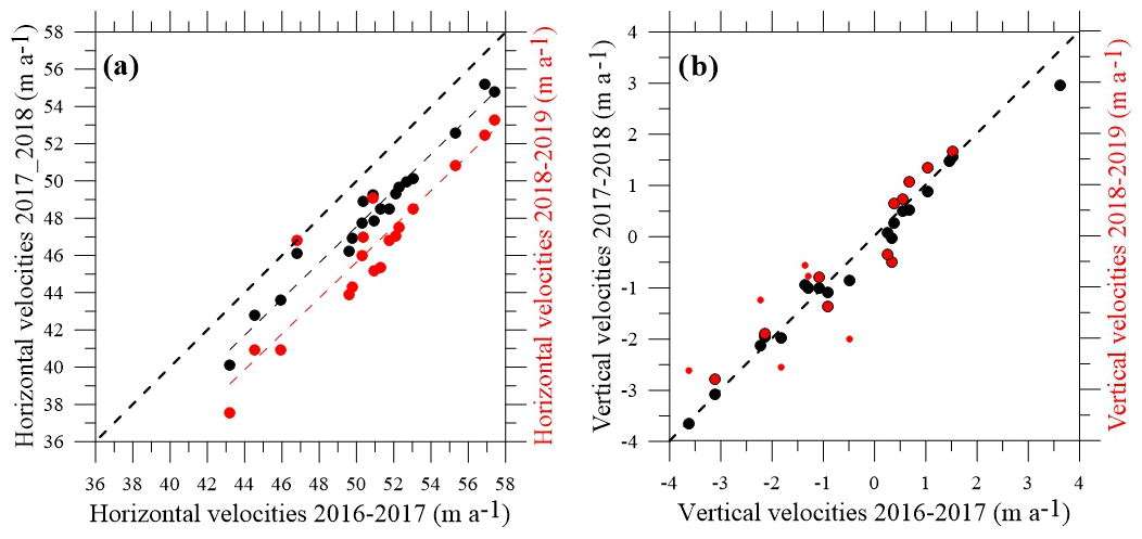
Figure 5 Comparison of horizontal ice flow velocities (a) and vertical velocities (b) between the years 2016/2017, 2017/2018 and 2018/2019. The black dots correspond to the comparison between the 2016/2017and 2017/2018 periods. The red dots correspond to the comparison between the 2016/2017 and 2018/2019 periods. The thick dashed line corresponds to the bisector and the thin dashed lines to the regression lines. The small dots in the figure on the right correspond to the stakes that were set up in 2018 at distances of more than 25 m from their initial positions.

5.2 Emergence velocities

The emergence velocities have been calculated from Eq. (2) for each stake and reported in Fig. 6. The slope was determined from the digital elevation model using UAV measurements. We compared the emergence velocities obtained each year at each stake location (Fig. 7). Unlike the vertical velocities, the differences between emergence velocities calculated over the 3 years reveal a standard deviation of 0.8 m w.e. a⁻¹. The value of emergence velocities is affected by large uncertainties related to the slope.

Combined with the measured thickness changes, the emergence velocity should make it possible to estimate the surface mass balance. However, our study shows that the uncertainties in the emergence velocity prevent us from calculating the point surface mass balance accurately. Indeed, the dispersion of 0.8 m w.e. a⁻¹ is large compared to the spatial variability of about 1 m w.e. a⁻¹ for point surface mass balance in the ablation zone of alpine glaciers (Vincent et al., 2018b).

For this reason, to calculate the surface mass balance, we suggest using the geodetic point surface mass balance described earlier rather than the emergence velocity.

Figure 6 Emergence velocities between the years 2016/2017, 2017/2018 and 2018/2019 (m a⁻¹).

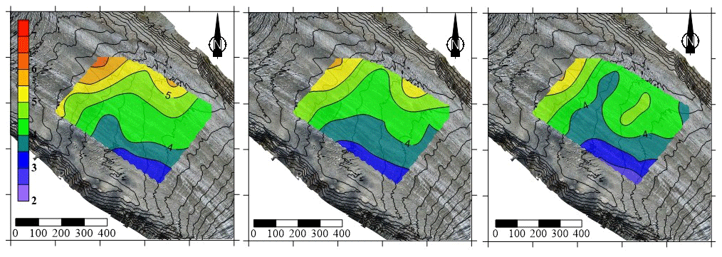
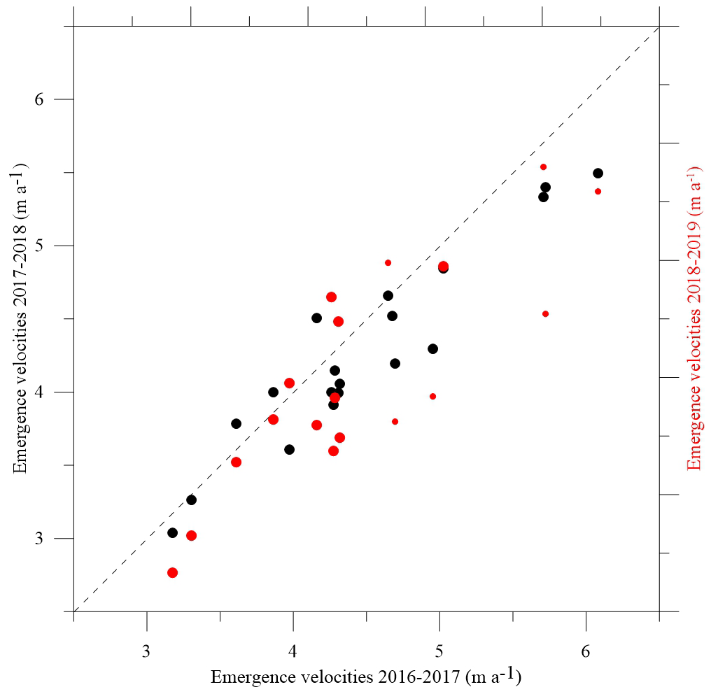
Figure 7 Comparison of emergence velocities between the years 2016/2017, 2017/2018 and 2018/2019. The black dots correspond to the comparison between the 2016/2017 and 2017/2018 periods. The red dots correspond to the comparison between the 2016/2017 and 2018/2019 periods. The red small dots correspond to the stakes that were set up in 2018 at distances of more than 25 m from their initial positions.

5.3 Geodetic point surface mass balances using in situ GNSS measurements

The geodetic point surface mass balance is calculated according to Eq. (4). We first tested the method in the studied region of the Argentière Glacier at 2400 m a.s.l. using the in situ GNSS measurements. For this purpose, we used the altitudes of the surface at the stake locations for the years 2017 and 2018 and the vertical velocities observed in 2016/2017. The resulting point surface mass balances for the hydrological year 2017/2018 are compared with the observed surface mass balances and plotted in Fig. 8a. Note that the surface mass balances are in m of ice per year. The comparison shows very good agreement. The maximum difference is 0.39 m of ice per year and the standard deviation is 0.20 m of ice or 0.18 m w.e. per year. In addition, we calculated the surface mass balances of 2018/2019 from the vertical velocities observed in 2016/2017 and 2017/2018 (Fig. 8b). In this case, the comparison with the observed surface mass balances shows large discrepancies. However, a more detailed analysis reveals that the calculated and observed surface mass balances are very similar if the vertical velocities observed in 2016/2017 and 2017/2018 were measured exactly at the same location as the stakes measured in 2018/2019. In Fig. 8b, the large dots show the calculated and observed surface mass balances for the stakes located within a distance no greater than 15 m. From this comparison, the differences are less than 0.5 m a⁻¹ of ice, and the standard deviation is 0.17 m of ice or 0.15 m w.e. a⁻¹.

From this analysis, we conclude that the geodetic point surface mass balance can be obtained with an accuracy of about 0.2 m w.e. a⁻¹ using the vertical velocities observed over the previous years. It requires the measurement of the horizontal ice flow velocity and the altitudes of the ends of the velocity vector exactly at the same location within a radius of less than 15 m compared to that of vertical velocity determination. In practice, the vertical velocities should be observed accurately between two years, t and t+1, from stakes and GNSS measurements. Then, for the following or previous years, the point surface mass balance can be obtained from surface measurements only (without drillings and setting new stakes) using the horizontal velocity and the altitudes of the surface measured at each end of the horizontal vector. In the next section, we examine how such measurements obtained from remote sensing data can also be used effectively to determine the point surface mass balance.

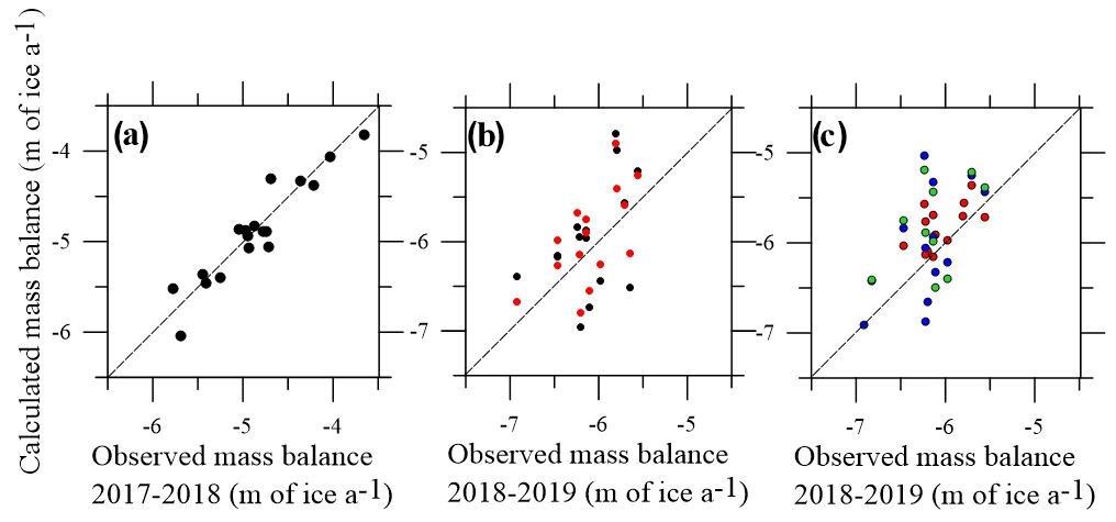
Figure 8 Observed and calculated point surface mass balances at 2350 m a.s.l. at Argentière Glacier. The point surface mass balances have been calculated (a) for the year 2017/2018 using the vertical velocities measured in 2016/2017 and elevations from GNSS measurements, (b) for the year 2018/2019 using the vertical velocities measured in 2016/2017 (black dots) and 2017/2018 (red dots) and elevations from GNSS measurements and (c) for the year 2018/2019 using elevations from remote sensing data (UAV data) and the vertical velocities measured in 2018/2019 (red dots), 2017/2018 (blue dots) and 2016/2017 (green dots). The large dots shown in Fig. 8b correspond to the stakes which were set up within a radius of less than 15 m.

5.4 Geodetic point surface mass balances using remote sensing measurements

Here, we used the same method described in the previous section. However, the in situ GNSS measurements used to determine the altitudes and horizontal velocities are replaced by remote sensing measurements. For this purpose, we used the horizontal velocities (Fig. 9) and the DEMs (Fig. 10) obtained from UAV surveys in 2018 and 2019. The vertical velocities are those observed in 2018/2019, 2017/2018 and 2016/2017. The horizontal velocities have been neglected for stakes 9 and 10 given the poor quality of the correlation and the opening and/or closing of crevasses in the ice (close to stake 10) that caused a drastic change between the photos, which subsequently affected the image correlation (Fig. 9).

Some details on the procedure are given below for the sake of clarity. The horizontal velocities retrieved from the UAV surveys were determined at positions where vertical velocities were measured. In this way, the coordinates XY of each vector end have been calculated (green dots in Fig. 9). Then we used the DEMs from 2018 and 2019 (Fig. 10) to determine the elevations of these points, Z_s1, 2018 and Z_s2,2019 (see Eq. 4 and Fig. 3). The comparison between the in situ horizontal velocities and the velocities obtained from the UAV surveys reveals a standard deviation of 0.7 m a⁻¹.

The reconstructed point surface mass balances are compared with the observed surface mass balances in Fig. 8c. For this reconstruction, we used the vertical velocities observed in 2018/2019 (red dots), 2017/2018 (blue dots) and 2016/2017 (green dots). For the reconstructions using the vertical velocities of 2016/2017 and 2017/2018, we excluded data from sites 1, 11, 12, 17, 18 and 19 for which the stakes were measured at distances of more than 30 m from those of 2018/2019.

The differences between the observations and the reconstructed surface mass balances using the 2018/2019 vertical velocities are less than 0.45 m of ice per year, and the standard deviation is 0.24 m of ice or 0.22 m w.e. a⁻¹. The differences between the observations and the reconstructed surface mass balances using the 2016/2017 and 2017/2018 vertical velocities show standard deviations of 0.42 and 0.40 m w.e. a⁻¹, respectively.

From these results, we conclude that the point surface mass balances can be obtained with an accuracy of about 0.3 m w.e. a⁻¹ using remote sensing measurements, assuming that the vertical velocities have been observed accurately over the previous years.

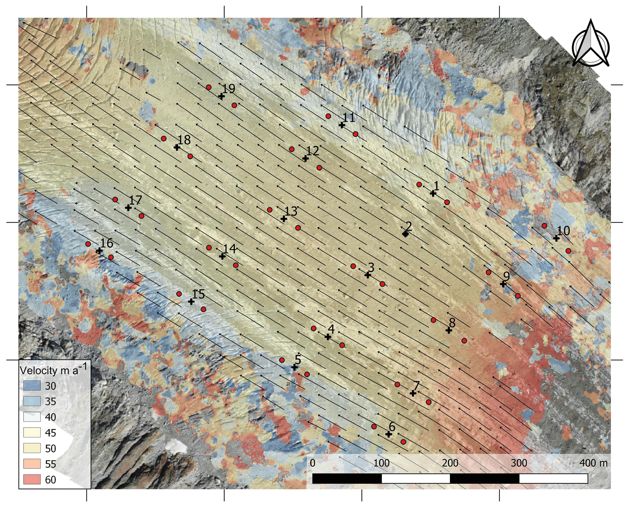
Figure 9 Horizontal velocities obtained from feature tracking (Cosi-Corr) using UAV images. The black crosses show the locations where the vertical velocities were observed. The red dots correspond to the ends of horizontal vectors for 2018/2019, determined from UAV images.

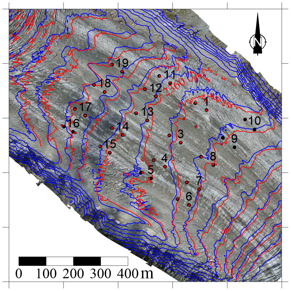
Figure 10 DEMs obtained from the UAV survey in 2018 (blue contour lines) and 2019 (red contour lines). The black dots correspond to the positions of the stakes in 2018 and 2019 observed from GNSS measurements. The red dots correspond to the ends of the horizontal velocity vectors obtained from UAV images.

5.5 Validation of the method: geodetic surface mass balances obtained in other regions

In order to establish that the results are neither accidental nor site-dependent, we tested the method on other areas of the Argentière Glacier and on another glacier, which is the Mer de Glace located approximately 10 km away (Fig. 1) and for which vertical velocities were available. Here, we used GNSS in situ measurements given that accurate elevation observations from remote sensing data are not available.

First, we selected two ablation stakes in a sector of the Argentière Glacier located at 2530 m a.s.l. These stakes were replaced within a radius of ±35 m each year between 2001 and 2018 (Fig. 1). Note that these measurements were not intended for vertical velocity determination but rather for point surface mass balance measurements. This explains why the stakes were not set up at exactly the same locations over the whole period. Note also that the region is not debris-covered and consequently the surface roughness is lower compared to the studied area at 2350 m. Using Eq. (4) and the method described in the previous section, we calculated the point surface mass balances at these two stakes over the period 2001–2018. For this purpose, we used the average vertical velocities calculated over this period. In addition, the altitudes of each stake for each year of this period have been observed. These two stakes (named stake 2 and stake 3) are located about 120 m apart. The average calculated vertical velocities are −0.24 m a⁻¹ (±0.44 m a⁻¹) and −0.79 m a⁻¹ (±0.33 m a⁻¹), respectively, and they did not show strong temporal changes (Fig. 11b). Note that the horizontal velocity decreased from 75 to 50 m a⁻¹ in this region between 2002 and 2018 (Fig. 11a). The geodetic point surface mass balances are compared to the observations (Fig. 12a). The standard deviations of the calculated and observed surface mass balance differences are similar to those of the vertical velocities (0.44 and 0.33 m a⁻¹, i.e. 0.4 and 0.3 m w.e. a⁻¹).

Second, we tested the method in another sector of the Argentière Glacier close to the equilibrium line which is located close to 2800 m a.s.l. For this purpose, we selected six stakes (stakes 7, 8, 9, 10, 11 and 12) which were measured along a longitudinal section between 2650 and 2750 m a.s.l. (Fig. 1) over the period 2005–2018. In this region, the horizontal ice flow velocity is about 50 m a⁻¹ (Fig. 11a). Here again, the network of stakes was mainly designed for point surface mass balance measurements. Thus, given that the stakes were set 10 m deep in the ice and the surface mass balance ranges between −4 and 0 m w.e. a⁻¹ depending on the year, the ablation stakes were not replaced each year. As the ablation stakes move with the ice flow, we selected only the measurements that were performed at the same locations. Indeed, after the first year following installation, the location of each stake was far from its initial position, and we cannot assume that the vertical velocity was similar. Consequently, 5 years are available to calculate the vertical velocities and to make the comparison between calculated and observed point surface mass balances (Fig. 12b). The standard deviations of calculated and observed point surface mass balance differences are 0.22 m of ice a⁻¹, i.e. 0.20 m w.e. a⁻¹.

Finally, we tested the method on another glacier, Mer de Glace (Fig. 1). On this glacier, we selected one stake at 2100 m a.s.l that was measured over 15 years between 2003 and 2018 (Vincent et al., 2018a). This ablation stake was set up each year at the same location within a radius of about 30 m. Using the method described in the previous sections, we calculated the point surface mass balances at this stake over the period 2003–2018. The average calculated vertical velocity is −1.10 m a⁻¹. Note that the horizontal velocity decreased from 80 to 50 m a⁻¹ and the thickness by 55 m in this region between 2003 and 2018. The results are plotted in Fig. 12c. The standard deviation of the calculated and observed point surface mass balance differences is 0.40 m w.e. a⁻¹.

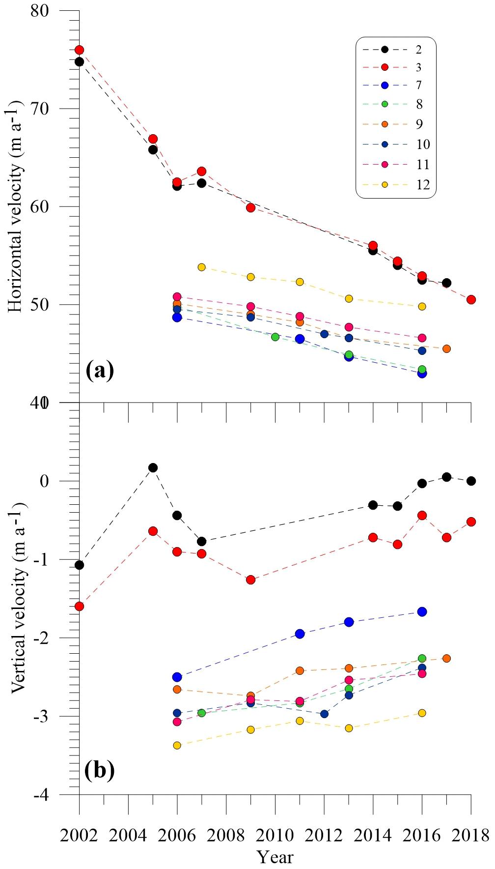
Figure 11 Horizontal (a) and vertical (b) velocities observed at the different stakes at 2550 m a.s.l. (stakes 2 and 3) and 2700 m a.s.l. (stakes 7, 8, 9, 10, 11 and 12).

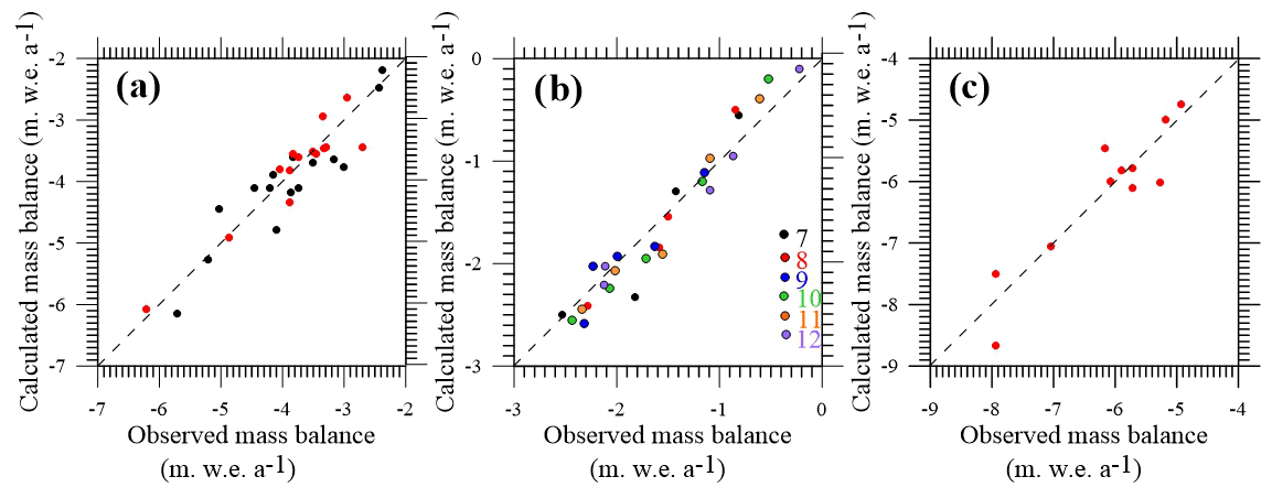
Figure 12 Observed and calculated point surface mass balances from (a) two ablation stakes located at 2550 m a.s.l. at Argentière Glacier measured between 2002 and 2018, (b) six stakes located at around 2700 m a.s.l. at Argentière Glacier measured between 2006 and 2017 and (c) one stake located at 2100 m a.s.l. on Mer de Glace glacier measured between 2003 and 2018.

6 Discussions

6.1 Point surface mass balance obtained from emergence velocities vs. vertical velocities

A classical approach to relate the point surface mass balance to thickness change is to use the emergence velocity (Cuffey and Paterson, 2010; Kääb and Funk, 1999). From this approach, the point surface mass balance is obtained from the sum of the emergence velocity and the thickness change (Eq. 1). However, the value of the mass balance reconstructed from the emergence velocity depends strongly on the selected surface slope and on thickness change, which both vary considerably with space and time. The value of the slope depends on the choice of the selected distance for the slope calculation and on the roughness of the surface.

In addition, the slope can change significantly from one year to the next. The emergence velocity is therefore not well-defined given that it depends strongly on the spatial and temporal changes in surface roughness, preventing an accurate determination of point surface mass balance, as shown in our study.

In contrast, in our analysis, we find that the changes in vertical velocity are insignificant over the 3 years of observations at 2350 m. From the other long series of observations, one can also see that they are small over decadal timescales. Thus, we propose to reformulate the emergence velocity formulation (Eq. 1) in order to express the point surface mass balance as a function of vertical velocity and altitude changes at the ends of the annual displacement vector (Eq. 4). In this way, provided that the vertical velocity has been assessed from in situ measurements over previous years, the point surface mass balance can be determined from remote sensing measurements alone outside the period of field measurements with no need of prescribing surface slope or elevation changes as required when using emergence velocities, which introduces significant uncertainties. Our results from the detailed studied area at Argentière Glacier (2350 m a.s.l.), for which the observations were designed to accurately determine the vertical velocity, demonstrate that the surface mass balance can be obtained from this method with an accuracy of about 0.2 m w.e. a⁻¹ from in situ GNSS measurements and about 0.3 m w.e. a⁻¹ using elevations and horizontal velocities obtained from very high-resolution remote sensing data acquired from UAV surveys.

6.2 Spatial and temporal variability in the vertical velocities

6.2.1 Analysis from observations

Our dataset shows that vertical velocities strongly vary in space over the glacier surface. Our detailed observations from the network used between 2016 and 2018 at the Argentière Glacier (2350 m) showed that the vertical velocity change can exceed 0.3 m a⁻¹ if the stakes are located at distances of more than 25 or 30 m (Sect. 5.1). We showed that the surface mass balance can be reconstructed with an accuracy of about 0.2 m w.e. a⁻¹ using the vertical velocities observed within a radius of less than 15 m. Records from the whole network suggest that the vertical velocity spatial gradient can exceed 1.5 m a⁻¹ per 100 m in this region. As a consequence, a horizontal deviation of 10 m could lead to a vertical velocity change exceeding the measurement uncertainty (0.15 m a⁻¹). To better assess the vertical velocity spatial gradient over length scales of 20 to 100 m, the vertical velocities have been calculated from 10 stakes set up in 2018/2019 on a longitudinal profile located between stakes 3 and 13 (Fig. 2). Note that the distances between these stakes are small, and they enable us to assess the vertical velocity variations at small scales. According to measurements shown in Fig. A1, the spatial gradient can reach up to 0.02 a⁻¹, which is slightly more important than what we found previously (0.015 a⁻¹). We can conclude that reconstructing surface mass balance from remote sensing requires measurements of the horizontal ice flow velocity and the altitudes of the ends of the velocity vector exactly at the same locations, i.e. within a radius of less than 15 m compared to that of vertical velocity determination.

The analysis of temporal changes also deserves particular attention. The 3 years of detailed observations performed at 2350 m at Argentière Glacier does not reveal temporal changes exceeding the measurement uncertainties, as shown in Fig. 5b. Note that the longer series of observations available to study the temporal changes over decadal timescales were not designed to measure the vertical velocities. However, from the longer series of observations performed at Argentière Glacier at 2550 and 2700 m a.s.l. (Fig. 11b), we assessed a general temporal trend of about 0.07 m a⁻². We can conclude that the past period over which the vertical velocities are determined should not exceed 4 years in order to not exceed an uncertainty of 0.3 m w.e. a⁻¹ on the reconstructed surface mass balance. This conclusion could be different with stronger temporal changes in vertical velocities. Further observations and analysis are needed to better estimate the temporal changes.

6.2.2 Analysis from numerical modelling

To analyse the spatial and temporal variabilities in the vertical velocities over the entire glacier, we performed 3D full-Stokes ice-flow simulations for two different glacier geometries using a surface DEM measured in 1998 and 2015 and reconstructed bedrock topography (Rabatel et al., 2018). The calculation is solved using the Elmer/Ice model (Gagliardini et al., 2013). The linear basal friction parameter is inferred from surface velocity and topography measurements made in 2003 (Berthier et al., 2005) using the adjoint-based inverse method (Gillet-Chaulet et al., 2012). For each given glacier geometry, we compute the corresponding flow solution and assume constant friction over time. Therefore, changes in velocity are only induced by changes in the glacier geometry between 1998 and 2015. We used an unstructured mesh with a 100 m horizontal resolution refined down to 10 m in the stake network monitoring area at 2400 m a.s.l.

By integrating the mass conservation equation for an incompressible fluid along the vertical axis, we can write the following:

$$\begin{array}{}\text{(5)}& w_{\mathrm{s}}=w_{\mathrm{b}}-{\int }_{z_{\mathrm{b}}}^{z_{\mathrm{s}}}{\displaystyle \frac{\partial u}{\partial x}}+{\displaystyle \frac{\partial v}{\partial y}}\mathrm{d}z,\end{array}$$

where w_b is the vertical velocity at the bed, z_s is the surface elevation, and z_b is the bed elevation. Vertical velocity at the surface can therefore be viewed as a sum of a component coming from sliding along the bedrock and a component coming from convergence/divergence of the ice flow integrated over the glacier thickness. For example, local depression in the bedrock topography creates negative vertical velocity w_b at the glacier base but also flow convergence that creates positive vertical velocity resulting in a smoothing of surface vertical velocity w_s by the ice deformation. Figure 13a shows the modelled vertical surface velocity in 2015. At the scale of the glacier, vertical surface velocities are spatially heterogeneous due to a combination of bedrock slope and the ice flux divergence/convergence (Fig. 13a). In the model, the basal vertical velocity w_b produced by ice flow along the bedrock can lead to small-scale variability in the basal vertical velocity that can be visible at the surface when sliding velocity is significant, as modelled around 2400 m a.s.l. in the studied stake network (Fig. 13a). Bedrock topography is therefore likely the origin of the observed pattern at 2400 m a.s.l. (Fig. 4). The pattern differences between the observations and the modelling results are likely due to bedrock elevation errors. Although the pattern of horizontal velocities is reproduced well (Fig. 13b), it seems difficult to properly reconstruct the vertical velocities.

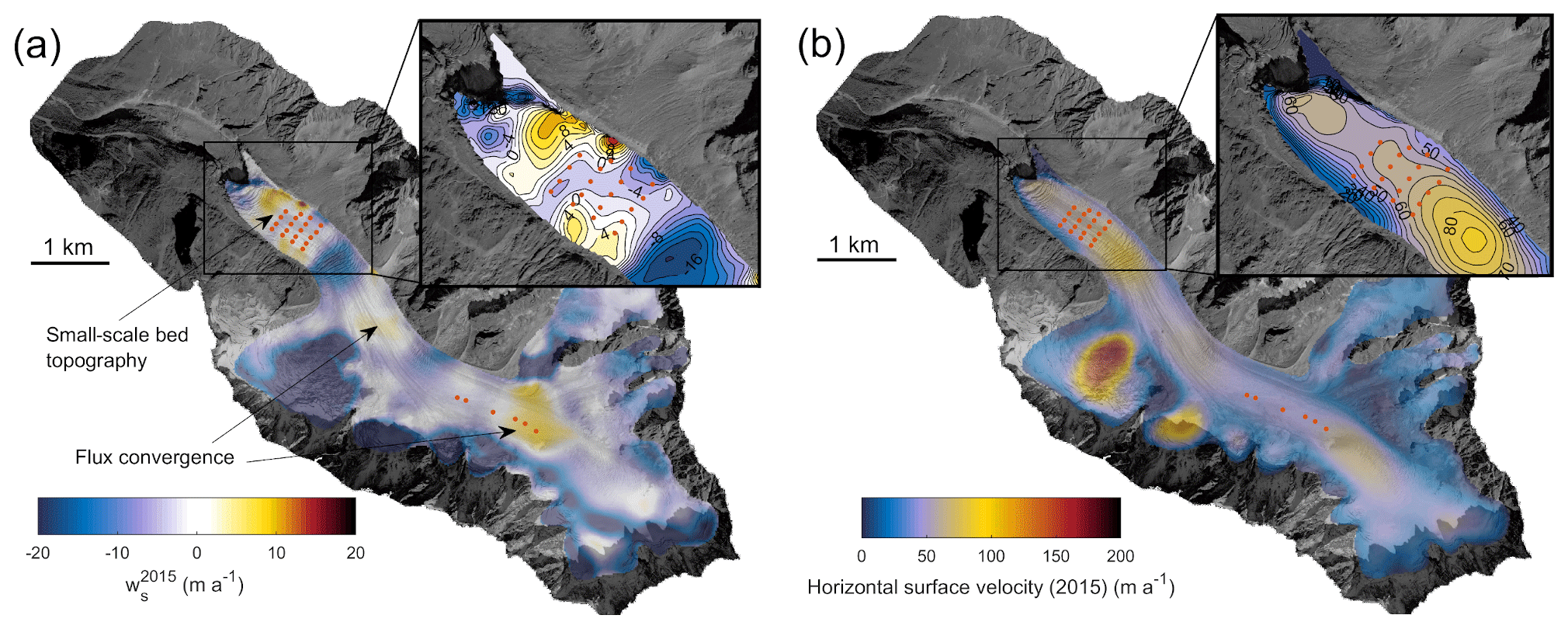
Figure 13 Vertical (a) and horizontal (b) surface velocities modelled at Argentière Glacier in 2015. Red dots show the locations of the ablation stakes set up at 2400 and 2650 m a.s.l.

Our numerical experiments were used to analyse the temporal changes in vertical velocities. We found that the response of the vertical velocities at the glacier surface to changes in glacier thickness over time is sensitive to the bedrock slope (averaged over a distance greater than the ice thickness). Consequently, a decreasing vertical velocity magnitude should be associated with decreasing horizontal velocities when bed slopes are significant (Fig. 14). However, the magnitude of small-scale (length-scale inferior to glacier thickness) spatial variations in vertical velocity due to bedrock topography seems to be little affected by the large change in horizontal velocities (Figs. 14 and 15). We show that reduced amplitude of w_b due to decreasing sliding speed is compensated for by the reduced amplitude of the ice flux convergence/divergence produced by bedrock anomalies (red arrows in Fig. 15). Bedrock depressions and bumps of sizes comparable to the glacier thickness produce, respectively, convergence and divergence in the ice flow, creating vertical velocities of opposite signs compared to the velocities created by sliding at the glacier base. These two components of the surface vertical velocity decrease in magnitude in response to thickness changes resulting in a limited change in the sum of the two components and therefore in surface vertical velocities. This results in nearly constant vertical velocity in which large-scale averaged bedrock slope is low, which explains why the observed pattern of surface vertical velocity (Fig. 4) is conserved well over time.

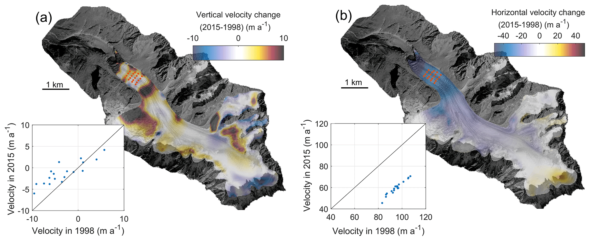
Figure 14 Modelled changes in vertical (a) and horizontal (b) surface velocities between 1998 and 2015. Insets compare modelled velocities at the stake location (orange dots) between 1998 and 2015.

In summary, at large scales, the magnitude of surface vertical changes over time are proportional to bedrock slope and changes in horizontal velocities, while at small scales, the spatial patterns tend to be conserved over time due to compensation between changes in bedrock vertical velocities and ice flux convergence/divergence. These findings suggest that our method is likely applicable only in areas of low bedrock slope.

Figure 15 Modelled changes in vertical velocities at the surface (a) and at the bedrock (b) between 1998 and 2015. The righthand figure (c) shows the change in vertical velocity at the surface due to changes in flow convergence/divergence. The red arrows indicate the locations where changes in basal vertical velocities are compensated for by flow convergence/divergence changes, resulting in constant surface vertical velocities.

Note that, in our study, we used the annual velocities measured at the end of the ablation season (from September to September) such that potential seasonal changes in the vertical and horizontal motion or in basal uplift and bed separation (e.g. Sugiyama et al., 2004; Nienow et al., 2005) are not expected to bias the geodetic annual surface mass balances obtained from the vertical velocities.

6.3 Uncertainties in geodetic point surface mass balances

The uncertainty related to the point surface mass balance determination results from uncertainties in the elevation measurements and in the vertical velocity. Using Eq. (4) and assuming the independence of the different sources of uncertainties, the overall uncertainty related to the reconstructed point surface mass balance is obtained by applying the method of error propagation and assuming uncorrelated errors:

$$\begin{array}{}\text{(6)}& {\mathit{\sigma }}_{\mathrm{b}}^{\mathrm{2}}=\mathrm{2}{\mathit{\sigma }}_z^{\mathrm{2}}+{\mathit{\sigma }}_w^{\mathrm{2}},\end{array}$$

in which σ_b, σ_z and σ_w are the uncertainties relative to the point surface mass balance, elevation and vertical velocity, respectively.

The uncertainty in elevation depends both on the method of XY positioning, the surface slope or roughness, and the method of altitude determination. Depending on the surface roughness, we can assess the elevations with an accuracy ranging from 0.1 to 0.3 m from UAV measurements, as shown in this study.

The uncertainty in vertical velocity is ±0.1 m a⁻¹, as mentioned in the Data section. However, additional uncertainty could come from the method of elevation observations for the bottom of the stakes. Indeed, the GNSS measurements are commonly related to the surface of the ice at the location of the stakes and not to the summit of the stakes. Consequently, the altitude of the bottom of each stake results from the difference between the altitude of the surface and the buried height of the ablation stake. Indeed, this determination is accurate only if the measurement of emergence has been performed exactly from the point on which the GNSS measurement was made. Unfortunately, in most cases, one operator held the stick of the GPS antenna at the ice surface close to the ablation stake, and another operator measured the emergence of the stake but not exactly from the surface altitude that corresponds to the bottom tip of the GPS antenna. Except for the measurements performed at 2350 m a.s.l between 2016 and 2019, which were designed for this purpose, this gives an additional uncertainty of ±0.1 m for the altitude of the bottom of the stake, i.e. ±0.14 m a⁻¹ for the calculated vertical velocity.

The overall uncertainty in the geodetic point surface mass balance obtained from remote sensing data is therefore estimated to range between ±0.20 and ±0.60 m a⁻¹ using accurate DEMs from UAV photogrammetry depending on the surface roughness and the method used for vertical velocity determination.

7 Conclusions

The classical way to determine the point surface mass balance in the ablation zone of a glacier is to set up ablation stakes and dig pits or conduct drillings in the accumulation zone. Here, we showed that, in the ablation zone, the point surface mass balances can be reconstructed from surface altitudes and horizontal velocities only, provided that the vertical velocities have been measured for at least 1 year in the past. Our method first requires accurate measurement of the vertical velocities between two years, t and t+1, from stakes and GNSS measurements. Then, for the following or previous years, the point surface mass balances can be obtained easily from surface measurements only using the horizontal velocity and the surface elevation at each end of the horizontal displacement vector (Eq. 4). These measurements can be obtained from remote sensing provided that the ice flow velocity and altitude determinations are sufficiently accurate.

Our method assumes that the annual vertical velocities are almost constant with time. We have used a numerical modelling study to show that this approximation holds in areas of low bedrock slope (averaged over a distance greater than the ice thickness). This is supported by our detailed observations performed on the Argentière Glacier at 2400 m a.s.l. and designed for this purpose. A comparison between the reconstructed point surface mass balances and the observed values shows close agreement. Further tests performed on datasets acquired in other regions of the Argentière and Mer de Glace glaciers show standard deviations of ±0.2 to ±0.4 m w.e. a⁻¹ between reconstructed and observed point surface mass balances despite the fact that these measurements were not designed for this purpose. For these tests, we used the averaged vertical velocities obtained over the last decade.

From our results, we conclude that the point surface mass balances can be obtained with an accuracy of about 0.3 m w.e. a⁻¹ using remote sensing measurements and assuming that the vertical velocities have been observed accurately over the previous years within a radius of less than 15 m. We also conclude from our datasets that the past period over which the vertical velocities are determined should not exceed 4 years in order to not exceed an uncertainty of 0.3 m w.e. a⁻¹ on the reconstructed surface mass balance, although further observations and analysis are needed to better estimate these spatial and temporal changes. Note that, for comparison, the measurement uncertainty related to the in situ measurements of point surface mass balance is 0.14 m w.e. a⁻¹ in the ablation zone (Thibert et al., 2008).

Given the recent improvements in satellite sensors, it is conceivable to apply our method using high-spatial-resolution satellite images like Pléiades or WorldView (0.5 m resolution). For these point surface mass balance reconstructions, note that, given the strong spatial variability in vertical velocity, it is crucial to determine the altitudes of the surface at each end of the horizontal displacement vector at the exact sites on which the vertical velocities are known. We conclude that our method could be useful to determine numerous point surface mass balances and reduce the amount of effort required to conduct field measurements, especially in remote areas.

Previous studies have shown that the point surface mass balance signal reveals a climatic signal that is unbiased by the dynamic glacier response, unlike the commonly used glacier-wide mass balance (Rasmussen, 2004; Huss et al., 2009; Eckert et al., 2011; Thibert et al., 2018; Vincent et al., 2017). In the glaciological community, there is growing awareness that point surface mass balance measurements are important basic data to be shared for mass balance and climate change analyses. In this respect, the World Glacier Monitoring Service has started collecting such data on a systematic basis as a complement to glacier-wide surface mass balances (WGMS, 2020). Our method should open up new prospects to obtain more numerous point surface mass balances in the future while reducing the amount of time and energy required for in situ measurements.

Another line of research not explored in the present study could also be examined. The method proposed in the present study requires the vertical velocity to reconstruct the annual point surface mass balance. However, if we derive Eq. (4) and assume that vertical velocity is constant with time, we can determine the surface mass balance changes instead of the absolute surface mass balances with the elevation determinations only. Assuming that satellite sensors provide sufficient accuracy in elevation and horizontal velocity, this method could be very helpful to reconstruct changes in surface mass balance in remote areas for which in situ measurements are very difficult. In this way, point surface mass balance changes in numerous unobserved glaciers could be considered with remote sensing observations only. This would make it possible to obtain climatic signals all over the world which are unbiased by dynamic glacier response.

Appendix A

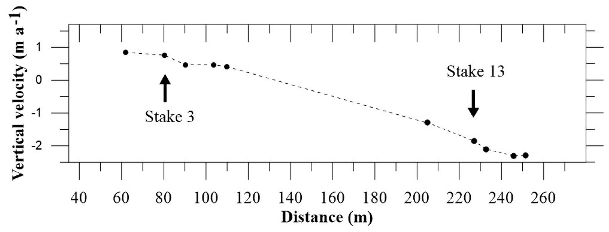
Figure A1 Vertical velocities obtained from 10 stakes measured in 2018/2019 on a longitudinal profile located between stakes 3 and 13 (see Fig. 2 for the locations of stakes 3 and 13).