Analysis of the surface mass balance for deglacial climate simulations

A realistic simulation of the surface mass balance (SMB) is essential for simulating past and future ice-sheet changes. As most state-of-the-art Earth system models (ESMs) are not capable of realistically representing processes determining the SMB, most studies of the SMB are limited to observations and regional climate models and cover the last century and near future only. Using transient simulations with the Max Planck Institute ESM in combination with an energy balance model (EBM), we extend previous research and study changes in the SMB and equilibrium line altitude (ELA) for the Northern Hemisphere ice sheets throughout the last deglaciation. The EBM is used to calculate and downscale the SMB onto a higher spatial resolution than the native ESM grid and allows for the resolution of SMB variations due to topographic gradients not resolved by the ESM. An evaluation for historical climate conditions (1980–2010) shows that derived SMBs compare well with SMBs from regional modeling. Throughout the deglaciation, changes in insolation dominate the Greenland SMB. The increase in insolation and associated warming early in the deglaciation result in an ELA and SMB increase. The SMB increase is caused by compensating effects of melt and accumulation: the warming of the atmosphere leads to an increase in melt at low elevations along the ice-sheet margins, while it results in an increase in accumulation at higher levels as a warmer atmosphere precipitates more. After 13 ka, the increase in melt begins to dominate, and the SMB decreases. The decline in Northern Hemisphere summer insolation after 9 ka leads to an increasing SMB and decreasing ELA. Superimposed on these long-term changes are centennial-scale episodes of abrupt SMB and ELA decreases related to slowdowns of the Atlantic meridional overturning circulation (AMOC) that lead to a cooling over most of the Northern Hemisphere.

1 Introduction

Increasing contributions to sea-level rise from the Greenlandic and Antarctic ice sheets have led to an enhanced interest in processes that explain past and future ice-sheet changes (see Fyke et al., 2018, for a recent review). Ice sheet mass changes are controlled by variations in the surface mass balance (SMB) and ice discharge (van den Broeke et al., 2009; Khan et al., 2015). The SMB is determined by mass gain due to accumulation as a result of snow deposition and mass loss by ablation induced by thermodynamical processes at the surface and subsequent meltwater runoff (Ettema et al., 2009). Other processes resulting in ice sheet mass changes are iceberg calving and basal melting at the ice–ocean and ice–bedrock interfaces.

To model the SMB, atmospheric processes associated with the energy balance at the surface, as well as snow processes, such as albedo evolution or refreezing, need to be simulated realistically (Vizcaíno, 2014). Therefore, most of the analyses on changes and variability in the SMB have been based on observations, statistical regression, and correction techniques, as well as simulations with high-resolution regional climate models (RCMs) which are constrained by reanalysis and Earth system model (ESM) data at the lateral boundaries, and cover the last century and near future only (e.g., Fettweis et al., 2008; Ettema et al., 2009; Hanna et al., 2011; Lenaerts et al., 2012; Fettweis et al., 2013; Box, 2013; Fettweis et al., 2017; Noël et al., 2018; Agosta et al., 2019; van Wessem et al., 2018). However, for long-term studies of past and future ice-sheet and climate changes, output from state-of-the-art ESMs is used directly. It is therefore essential that ESMs are able to realistically simulate the SMB. This is specifically challenging as ESMs exhibit biases and the horizontal resolution is often not sufficient to capture small-scale climate features, e.g., sharp topographic gradients at the ice-sheet margins, as well as cloud, snow, and firn processes (e.g., Lenaerts et al., 2017; van Kampenhout et al., 2017; Fyke et al., 2018).

In this study, SMBs are derived from transient simulations of the last deglaciation with the Max Planck Institute for Meteorology ESM (MPI-ESM) using an energy balance model (EBM). The EBM accounts for the energy balance at the surface, including snow processes, such as albedo evolution or refreezing, and has been shown to result in a more realistic representation of ice volume changes than other methods (e.g., positive degree day models; e.g., Tarasov and Richard Peltier, 2002; Abe-Ouchi et al., 2007; Bauer and Ganopolski, 2017). To thoroughly evaluate the SMBs derived with this setup, the EBM is also applied to MPI-ESM simulations of the recent historical period (1980–2010) and compared to Greenland SMBs from regional modeling.

This study extends the analysis of Northern Hemisphere SMB changes to the last deglaciation (21 ka to present). The last deglaciation was characterized by significant changes in insolation and associated changes in greenhouse gas concentrations, ice sheets, and other amplifying feedbacks (Clark et al., 2012). The large ice loss resulted in the disappearance of the North American and Eurasian ice sheets. In the Northern Hemisphere, only the Greenland ice sheet remains at present. The retreat of the ice sheets during the deglaciation resulted in about a 1 m sea-level rise per 100 years, a rate which on average is comparable to future projections of sea-level rise (e.g., Horton et al., 2014). The collapse of the ice sheets also resulted in significant changes in the atmospheric and oceanic circulation, as well as associated climate features (e.g., Löfverström and Lora, 2017). Orographic changes induced by the decrease in the Laurentide and Cordilleran ice sheets led to changes in the Northern Hemisphere stationary wave patterns and thereby the North Atlantic jet stream, which significantly affected the Northern Hemisphere climate (e.g., precipitation and temperature patterns; Andres and Tarasov, 2019; Lofverstrom, 2020; Kageyama et al., 2020). Superimposed on these long-term changes were periods of abrupt climate events. Some of the most prominent events are Heinrich event 1 (HE1; about 16.8 ka; e.g., Heinrich, 1988; McManus et al., 2004; Stanford et al., 2011) and the Younger Dryas (about 13–11.5 ka; Carlson et al., 2007), both of which are associated with a major Northern Hemisphere cooling and a significant decrease in the Atlantic meridional overturning circulation (AMOC; e.g., Keigwin and Lehman, 1994; Vidal et al., 1997). The significant climate changes and the variability associated with changes in the Northern Hemisphere ice sheets during the deglaciation emphasize the need for a realistic representation of the SMB for past and future stand-alone ice sheet and coupled climate–ice-sheet model simulations (Fyke et al., 2018).

The main aim of this paper is to introduce the EBM and apply it to long-term climate simulations. First, we introduce the EBM and the underlying simulations with the MPI-ESM. Second, we provide a thorough evaluation of the model performance for present-day climate conditions over Greenland by comparing the derived SMB data set to SMBs from regional climate modeling. We then present and investigate changes and variability in the SMB and equilibrium line altitude (ELA) throughout the last deglaciation and point out mechanisms behind the SMB and ELA changes. Here, we aim at exploring SMB and ELA changes under a transient climate forcing in order to understand the mechanisms behind their variability at glacial timescales. As the SMB is a key parameter in controlling changes in the geometry of the ice sheets, this data set is available to the ice-sheet modeling community along with other forcing fields required for ice-sheet model simulations.

2 Model systems and data

To obtain SMB fields from long-term climate simulations, the MPI-ESM is used in combination with an EBM. Two kinds of simulations were performed. First, a set of historical simulations (1980–2010) were performed to evaluate the EBM-derived SMBs. For this, we force the EBM with output from historical simulations with MPI-ESM and ERA-Interim reanalysis and compare the obtained SMBs to output from the regional climate model MAR (Modèle Atmosphérique Régional; Fettweis, 2007). Second, simulations of the last deglaciation with prescribed ice-sheet boundary conditions were performed to investigate SMB changes under transient climate forcing. The simulations performed for this study are summarized in Table 2.

2.1 The surface energy and mass balance model

We use the EBM to calculate and downscale the SMB from the coarse-resolution atmospheric model grid of MPI-ESM onto high-resolution ice-sheet topographies. The main challenge in downscaling the SMB is to realistically capture the small-scale features of both melt and accumulation. Melt and accumulation are highly dependent on the topographic height; e.g., at a given time, low elevations might experience melt, while higher elevations remain frozen. Projecting melt and accumulation on a topography with better-resolved vertical gradients has therefore a significant impact on the SMB. Hence, differences between the original and downscaled SMBs are mainly a result of differences in the elevation rather than the horizontal grid refinement. To account for this, we employ a 3-D EBM scheme that is forced with high-frequency atmospheric data. The EBM scheme is an enhanced version of the energy and mass balance code that has been used to couple the ice-sheet model SICOPOLIS to a previous version of MPI-ESM (Mikolajewicz et al., 2007; Vizcaíno et al., 2008, 2010). The main improvements are (1) an advanced broadband albedo scheme considering aging, snow depth dependency, and the influence of the cloud coverage on the thermal radiation, (2) the consideration of snow compaction and the vertical advection of snow and ice properties, (3) rain-induced change in the heat content of the snow layers, and (4) an enhanced refreezing scheme. We further adapted the scheme by introducing elevation classes, following Lipscomb et al. (2013). Calculating the SMB on fixed elevation levels has the advantage that the model becomes computationally cheaper and that the obtained 3-D fields can be interpolated onto different ice-sheet topographies (see Sect. 2.3). Note that an elevation dependence of the SMB components is a simplified assumption and valid mainly for present-day Greenland. Atmospheric dynamics also significantly contribute to variations in the SMB components, specifically over present-day Antarctica. In the following, we present the basic structure of the EBM, including its improvements compared to the scheme used in Vizcaíno et al. (2010).

2.1.1 Height correction

To compute the SMB, atmospheric fields are mapped onto 24 fixed elevation levels, ranging from sea level to 8000 m (we use irregular intervals that start with 100 m distance at the surface and increase with height; see Table A1). To account for height differences between each of these elevation classes and the surface elevation of the atmospheric model, a height correction is applied to near-surface air temperature, humidity, dew point, precipitation, downward longwave radiation, and near-surface density fields. The downward shortwave radiation is kept constant as it is largely affected by atmospheric properties independent of elevation differences (e.g., ozone concentration, aerosol thickness; Yang et al., 2006).

The following height corrections are applied before the EBM calculations.

• Total precipitation rates (liquid and solid) are corrected in consideration of the height-desertification effect. This halves the precipitation for an orography height difference of 1000 m above a threshold height of 2000 m for each grid point (Budd and Smith, 1981). Note that snowfall is determined from the total precipitation for height-corrected near-surface air temperatures below 0 ^∘C within the EBM.

• Near-surface air temperature and dew point are corrected using a constant lapse rate of −4.6 K km⁻¹, similar to the value proposed in Abe-Ouchi et al. (2007). The specific humidity, which can be used as an alternative to the height-corrected dew-point temperature to calculate the latent heat flux (Bolton, 1980), is decreased with height under the assumption that the relative humidity stays constant throughout the atmospheric column.

• The surface pressure is adjusted under the assumption of a typical atmospheric density and pressure profile $p=p_{\mathrm{atm}\mathrm{0}}\exp (-z/H_{\mathrm{s}})$, where p_atm0 is the pressure at the surface, z is the height, and H_s is the scale height with a typical value of 8.4 km.

• The downward longwave radiation is corrected by applying the observed constant radiation gradient of Marty et al. (2002) and is reduced by 29 W m⁻² km⁻¹ (see also Wild et al., 1995).

2.1.2 Surface mass and energy balance calculation

Accumulation and melt determine the SMB. Accumulation is controlled by precipitation and takes place if precipitation falls as snow. In the EBM, precipitation is considered as snow with a density of 300 kg m⁻³ when the height-corrected near-surface air temperature is lower than the freezing temperature of 273.15 K. Otherwise, precipitation falls as rain.

The computation of melt requires a snow and/or ice model as the melt rate depends on the heat content of snow and the heat exchange between the surface snow layer and the atmosphere above, as well as the snow and/or ice layers below. To account for this, the EBM includes a five-layer snow model discretized into layers of increasing thickness. The model considers only vertical exchanges because the horizontal extent is several orders of magnitude larger than the vertical extent. The snow model starts initially with a reference density describing the typical exponentially increasing density with depth (Cuffey and Paterson, 2010). The top layer's exchange with the atmosphere is computed from short- and longwave radiation fluxes, latent and sensible heat fluxes, and the heat release due to the immediate refreezing of rain if the surface layer has a temperature below the freezing temperature. Latent and sensible heat fluxes are calculated from the height-corrected variables using bulk aerodynamic formulas. The temperature of rain is assumed to be equal to the height-corrected near-surface air temperature. After updating the heat content of the surface layer, the temperature difference from the layer below determines the heat flux into the layer below by taking density-dependent heat conductivity into account (Fukusako, 1990). The heat conductivity is a function of density following Schwerdtfeger (1963). We neglect any temperature dependence of ice or snow conductivity (Fukusako, 1990). The scheme progresses downward until the lowest layer is updated. The heat flux beyond the lowest layer is assumed to be zero, in agreement with observations showing that the ice or snow layer temperature below 10 m follows the long-term trend and not the seasonal cycle (Hooke, 2005). If the ice or snow layer's temperature exceeds the melting temperature, the temperature is set to the freezing point, and the related temperature excess converts the corresponding amount of ice or snow into liquid water. Liquid water penetrates into the layer below and refreezes in this layer as long as the layer is colder than the freezing temperature. Water refreezes as ice with a density of 917 kg m⁻³. As a consequence, the layer's density grows in consideration of mass conservation and eventually reaches the density of ice. Any remaining liquid water may penetrate further downward and potentially refreezes in the layers below. Liquid water that leaves the lowest layer or flows into a layer with a density exceeding the pore close density of 830 kg m⁻³ (Pfeffer et al., 1991) is treated as run-off and leaves the system. Moreover, refreezing of meltwater heats the layer by the release of latent heat, bringing the layer's temperature closer to the freezing point temperature. This process eventually terminates refreezing. Rain that precipitates on the surface can also percolate into lower layers, where it is treated as meltwater.

2.1.3 Albedo evolution

The amount of incoming radiation which is available for heating the snow/ice layers and eventually melting is controlled by the surface albedo α. The albedo parametrization used here differs from Vizcaíno et al. (2010). We have developed a frequency-independent broadband albedo that combines existing parameterizations, as described in this section. It represents processes neglected in conventional parameterizations and covers a broader range of albedos suggested by observational accounts. Note that all depths presented in the following are water equivalent (w.e.) depths (reference density of 1000 kg m⁻³).

Table 1 List of constants used in the albedo scheme as part of the EBM. Please see Sect. 2.1 for further details.

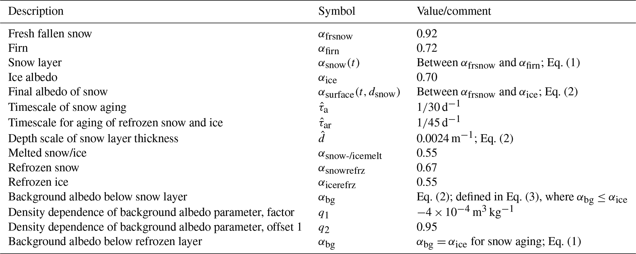
Freshly fallen snow has (in our scheme) an albedo of 0.92 (α_frsnow; see Table 1). Snow metamorphosis processes that change the snow's characteristics through the growth of larger crystals at the expense of smaller ones ultimately transform snow into firn (Cuffey and Paterson, 2010). As a result the snow albedo, α_snow(t), decreases and approaches the albedo of firn, α_firn, which is parameterized by a time-dependent exponential decay (Klok and Oerlemans, 2004; Oerlemans and Knap, 1998) as

$$\begin{array}{}\text{(1)}& {\mathit{\alpha }}_{\mathrm{snow}}\left(t\right)={\mathit{\alpha }}_{\mathrm{firn}}+\left({\mathit{\alpha }}_{\mathrm{frsnow}}-{\mathit{\alpha }}_{\mathrm{firn}}\right)\exp \left(-t_{\mathrm{snow}}{\widehat{\mathit{\tau }}}_{\mathrm{a}}\right),\end{array}$$

where t_snow is the time since the last snowfall and ${\widehat{\mathit{\tau }}}_{\mathrm{a}}$ a time constant (see Table 1). This process is here referred to as “aging”. Moreover, the depth of the top snow layer, d_snow(t), determines how much of a potentially darker background shows through and modulates the surface albedo (Klok and Oerlemans, 2004; Oerlemans and Knap, 1998). The equation

$$\begin{array}{}\text{(2)}& \begin{array}{rl}{\mathit{\alpha }}_{\mathrm{surface}}\left(t,d_{\mathrm{snow}}\right)& ={\mathit{\alpha }}_{\mathrm{snow}}\left(t\right)+\left({\mathit{\alpha }}_{\mathrm{bg}}-{\mathit{\alpha }}_{\mathrm{snow}}\left(t\right)\right)\\ & \times \exp \left(d_{\mathrm{snow}}/\widehat{d}\right)\end{array}\end{array}$$

renders this process, where α_bg is the background albedo, which is generally the albedo of ice, and $\widehat{d}$ is 0.0024 m⁻¹. In the albedo parameterization, melting reduces the snow thickness, while snowfall increases the thickness when the precipitation rate exceeds 7.23 × 10⁻¹⁰ m w.e. s⁻¹ ≈ 2.5 cm w.e. a⁻¹. The maximum snow depth is set to 2 m w.e., which corresponds to approximately 6 m of snow. Any additional snow is still considered in the layer model to close the mass calculation, but it does not impact the albedo (the snow depth is an internal diagnostic variable).

Depending on the snow depth, melting and refreezing surfaces have different albedo values (Table 1). If the snow depth lies above or below a snow depth threshold of 0.25 cm, the albedos for snow and ice are used, respectively. When the surface experiences melt, the albedo drops to the albedo of snow or ice melt (α_{snow-/icemelt}). When the surface refreezes, the albedo potentially increases (α_snowrefrz or α_icerefrz), and the aging process starts. The aging process is similar to that for snow processes as described in Eq. 1, but the albedos for refrozen surfaces are smaller (${\mathit{\alpha }}_{\mathrm{snowrefrz}/\mathrm{icerefrz}}$; the reference albedo α_firn reduces to ${\mathit{\alpha }}_{\mathrm{refrz}}=(\mathrm{2}\cdot {\mathit{\alpha }}_{\text{snowrfz/icerefrz}}+{\mathit{\alpha }}_{\text{snowmelt/icemelt}})/\mathrm{3}$ for refrozen snow or ice). Additionally, the process is slower (${\widehat{\mathit{\tau }}}_{\mathrm{ar}}$). Only melted surfaces and the background do not experience any aging.

Moreover, the background albedo shows a slight density dependence which impacts regions of persistent high melting and lowers the surface albedo via the background albedo. The background albedo is

$$\begin{array}{}\text{(3)}& {\mathit{\alpha }}_{\mathrm{bg}}=min\left({\mathit{\alpha }}_{\mathrm{ice}},q_{\mathrm{1}}\mathit{\rho }+q_{\mathrm{2}}\right),\end{array}$$

where $q_{\mathrm{1}}=-\mathrm{4}\times {\mathrm{10}}^{-\mathrm{4}}$ m³ kg⁻¹ and q₂=0.95, which is similar to values published by Liston et al. (1999); see also Suzuki et al. (2006) for another example of this kind of parameterization.

Furthermore, as part of our broadband albedo parameterization, we let varying cloud cover affect the surface albedo (Greuell and Konzelmann, 1994) because a higher cloud cover reflects more thermal radiation downward, which shifts the broadband albedo towards lower values (darker surface). We use the linear function of Greuell and Konzelmann (1994) so that the maximum albedo change is 0.1 between a complete overcast sky and cloud-free conditions.

All albedo values used in this study (e.g., for refrozen snow/ice, fresh snow, ice, firn) are tuned for a realistic representation of the SMB for historical climate conditions (see Sect. 3) and are listed in Table 1. The same parameters were applied in an EBM simulation forced with output from a high-resolution MPI-ESM simulation for historical climate conditions within the scope of SMB model inter-comparison (Fettweis et al., 2020). The results showed that the derived SMBs were very similar to observations in terms of the SMB mean climate, as well as the SMB trend (2003–2012).

2.1.4 Vertical advection and density evolution

For a non-zero SMB, the thickness of the uppermost layer of the snow model would change. To compensate for that, a simple 1-D advection scheme conserving heat and mass is applied. In the case of surface ablation, the densities and temperatures are advected upward. As the lower boundary condition, we assume an inflow of ice with a density of 917 kg m⁻³ and a temperature of the lowest model layer. In the case of accumulation, an inflow of snow with a density of 300 kg m⁻³ and a temperature of the height-corrected near-surface air temperature is assumed as the upper boundary condition. To account for snow compaction, we introduce the aforementioned reference density profile (Cuffey and Paterson, 2010). If the density of the downward-advected snow into a layer is smaller than the reference density in that layer, the density of the advected snow is set to the reference density, and the flow to the layer below is reduced accordingly to conserve mass. Once the reference density is reached in all layers, mass flows out of the bottom layer and is removed from the system. As a consequence of this procedure, the density in each layer lies always between the reference density (in the case of permanent snow accumulation) and the density of pure ice (in the case of permanent ablation).

2.2 The Max Planck Institute Earth System Model

The simulations in this study are performed with the Max Planck Institute for Meteorology Earth System Model (MPI-ESM, version 1.2; see Mikolajewicz et al., 2018; Mauritsen et al., 2019), consisting of the spectral atmosphere general circulation model ECHAM6.3 (Stevens et al., 2013), the land surface vegetation model JSBACH3.2 (Raddatz et al., 2007), and the primitive equation ocean model MPIOM1.6 (Marsland et al., 2003). Two different resolutions are used for the simulations. (1) For calculating the SMB over the last deglaciation, MPI-ESM is used in its coarse-resolution (CR) setup, hereafter referred to as MPI-ESM-CR. In this setup, ECHAM6.3 has a T31 horizontal resolution (approx. 3.75^∘) with 31 vertical hybrid σ levels which resolve the atmosphere up to 0.01 hPa (Stevens et al., 2013), and MPIOM1.6 has a nominal resolution of 3^∘ with two poles located over Greenland and Antarctica (Mikolajewicz et al., 2007). The selected setup is a compromise between computational feasibility and model resolution. (2) We additionally use a simulation with the low-resolution version of MPI-ESM1.2, hereafter referred to as MPI-ESM-LR, in which ECHAM6.3 has a T63 spectral grid (approx. 1.88^∘) with 47 vertical levels, and MPIOM features a 1.5^∘ nominal resolution. For model details, see Mauritsen et al. (2019).

2.3 Transient MPI-ESM climate simulations

We performed different simulations with the MPI-ESM-CR setup: (1) simulations to investigate the SMB throughout the last deglaciation, starting at 26 ka until the present (here, defined as 1950), and (2) simulations to evaluate the SMB for historical climate conditions (see Table 2). For the deglaciation experiment, the model was started from a spun-up glacial steady state and integrated from 26 ka until the year 1950 with prescribed atmospheric greenhouse gases (Köhler et al., 2017) and insolation (Berger and Loutre, 1991). The ice sheets and surface topographies were prescribed from the GLAC-1D (Tarasov et al., 2012; Briggs et al., 2014) reconstructions (Kageyama et al., 2017, see standardized PMIP4 experiments). We focus our analysis on the last 21 kyr of the simulation. Hereafter, this simulation is referred to as MPI-ESM-CR deglaciation experiment. All forcing fields are prescribed every 10 years and initiate changes in the topography and glacier mask, as well as modifications of river pathways, the ocean bathymetry, and the land–sea mask (Riddick et al., 2018; Meccia and Mikolajewicz, 2018). Freshwater from changing ice sheets is calculated from the thickness changes in the ice-sheet reconstructions for each grid point. For grid cells over land, meltwater is distributed through the hydrological discharge model, and over ocean it is discharged into the adjacent ocean grid cells. Ocean cells that become land due to changes in the sea level are initialized with the same vegetation form as the adjacent grid cells, while land cells that are deglaciated are covered with bare soil. After this initialization, the vegetation of the grid cells evolves interactively with JSBACH. Anthropogenic forcing, such as land use, is turned off in this simulation. For calculating the SMB, relevant variables of the atmospheric component of MPI-ESM1.2 are written out hourly throughout the simulation. Using the obtained atmospheric fields within the EBM (see Sect. 2.1) results in 3-D SMB fields which are then interpolated onto the GLAC-1D topography and ice mask (Tarasov et al., 2012). Computing a 3-D SMB also allows us to calculate the equilibrium line altitude (ELA), the elevation at which the SMB equals zero. At heights above the ELA, it is thermodynamically possible to accumulate snow throughout the year and form an ice sheet or glacier. At elevations below the ELA, melt dominates accumulation, and no ice sheet can form. Here, the ELA is calculated in each grid point, hence, resembling a potential ELA. It is a proxy for climate changes affecting the ice sheets. As the ELA estimate is calculated on the native model grid, it is more consistent with the model physics and boundary conditions used in the simulations than the downscaled SMB. Hence, integrated values of the ELA are less sensitive to changes in the ice-sheet mask than those of the SMB.

Table 2 Simulations performed, as described in Sect. 2.3. For the deglaciation experiments, the topography and ice sheets are taken from reconstructions and change throughout the simulation. For the historical and last millennium simulations, those fields remain constant through time.

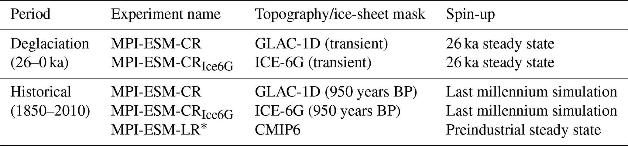
^∗ This simulation contributed to CMIP6 (see Sect. 2.3).

For the evaluation of the derived SMBs under historical climate conditions, we branched off a last millennium simulation at 950 years BP (years before present) from the deglaciation experiment. Within PMIP, last millennium simulations are used to provide a seamless transition between the last deglaciation and the historical period (Jungclaus et al., 2017). For the simulation, topography, land–sea and glacier masks, river pathways, and the ocean bathymetry are taken from the deglaciation experiment and kept constant at 950 years BP. Other forcing fields are adopted according to the PMIP3 standard protocol for the last millennium simulations (Schmidt et al., 2012) and updated every year. The forcing fields for the years 1850 to 2010 are taken from the CMIP6 simulations (see Mauritsen et al., 2019). For the years beyond 2010, the forcing fields in the desired resolution were not available at the time of the analysis. Overall, the applied forcing allows for a more realistic treatment of atmospheric processes associated with changes in, e.g., ozone, aerosols, CO₂ concentrations, and land use, and it accounts for their climatic impacts for present-day climate conditions. Specifically, we apply time-varying greenhouse gases (CO₂, N₂O, CH₄), volcanic forcing, ozone, tropospheric aerosols, and land-cover changes (see Jungclaus et al., 2010; Mauritsen et al., 2019). For the evaluation, only the years 1980–2010 are used, which allows for a sufficient adjustment of the model to changes in the forcing. We hereafter refer to this simulation as the MPI-ESM-CR historical experiment. Note that changes in the topography due to ice sheets are small between 950 years BP and 2010. Hence, we expect only a minor impact on the obtained SMBs.

Additionally, we performed a deglacial, last millennium, and historical simulation in which ice sheets and topographies are prescribed from ICE-6G reconstructions (Peltier et al., 2015), an alternative reconstruction often used as boundary forcing in deglacial simulations (Kageyama et al., 2017). Results from these simulations, hereafter referred to as MPI-ESM-CR_Ice6G experiments, are shown in Appendix A1 and emphasize differences in the SMB and relevant fields due to different ice-sheet boundary conditions. While the SMB response to the climate forcing in these simulations is qualitatively similar to the MPI-ESM-CR simulations forced with GLAC-1D reconstructions, differences in the freshwater runoff between the reconstructions lead to a different climate response in the model simulations.

For a thorough evaluation of the EBM and in order to investigate the effect of model resolution on the historical SMB, we additionally calculate the 3-D SMB fields from a CMIP6 (Wieners et al., 2019) historical simulation with the MPI-ESM-LR setup (see Sect. 2.2; Mauritsen et al., 2019; Wieners et al., 2019). The simulation allows us to further evaluate the EBM and to investigate differences in SMBs in regards to the spatial model resolution, as well as differences due to the underlying topographies. This simulation is hereafter referred to as MPI-ESM-LR historical experiment.

The 3-D fields derived for all historical control simulations are 3-dimensionally interpolated onto the ISMIP6 topography and masked with the ISMIP6 ice mask (see Sect. 2.4; Nowicki et al., 2016; Fettweis et al., 2020).

2.4 Evaluation data

To evaluate the EBM with respect to the atmospheric forcing data and its resolution, we additionally force the EBM with ERA-Interim reanalysis data from the European Center for Medium-Range Weather Forecasts (ECMWF; Dee et al., 2011). ERA-Interim was chosen as it is used as boundary forcing in the RCM simulations, which are used for a more thorough evaluation and are introduced at the end of this section. For comparison, we interpolate the ERA-Interim derived 3-D SMB fields onto the ISMIP6 topography and mask it with the ISMIP6 ice mask (see Sect. 2.3). ERA-Interim is available as 6-hourly data at a 0.75^∘ × 0.75^∘ horizontal resolution. ERA-Interim assimilates a great fraction of in situ and remote sensing observations, making it one of the best reanalysis products available (Cox et al., 2012; Zygmuntowska et al., 2012). However, as reanalysis data sets are model products, they exhibit biases specifically for variables associated with small-scale processes and areas where in situ observations are sparse (e.g., precipitation, clouds; Stengel et al., 2018). These biases are not unique to ERA-Interim but can be found in other reanalyses (Miller et al., 2018). Relevant biases for this study are discussed in Sect. 3.

Additionally, we compare the obtained SMB data sets from the MPI-ESM historical experiments to SMBs derived with MAR (version 3.9.6). For a detailed description of MAR and its setup, see Fettweis et al. (2017, 2020). The MAR simulation used in this study was run at a 15 km horizontal resolution with ERA-Interim boundary forcing (Dee et al., 2011) and interpolated onto the ISMIP6 topography (Nowicki et al., 2016), as described in Fettweis et al. (2020).

3 Greenland surface mass balance under historical climate conditions

For the Greenland ice sheet, a thorough evaluation of the accumulation and surface energy budget that determines surface melt is conducted under historical climate conditions (1980–2010). Variables derived from the EBM simulations forced with output from ERA-Interim and the historical MPI-ESM simulations are compared to SMBs from MAR. SMB, accumulation, and melt data sets are presented on the same ISMIP6 topography (see Sect. 2.3 and 2.4). In the following, accumulation is defined as mass gain due to snow deposition and melt as mass loss due to ablation (often referred to as runoff). Refreezing processes are considered in the melt estimate (see Sect. 2.1). All variables obtained using the EBM are hereafter referred to as EBM_MPI-ESM-CR, EBM_MPI-ESM-LR, and EBM_ERAI for the EBM simulations forced with the historical simulations of both MPI-ESM in coarse (CR) and low (LR) resolution and ERA-Interim reanalysis. The annual mean SMB averaged over 1980–2010 and the Greenland integrated value are shown in Fig. 1 and Table 3 for each of the simulations. The corresponding plots for the MPI-ESM-CR_Ice6G simulation are shown in Fig. A1.

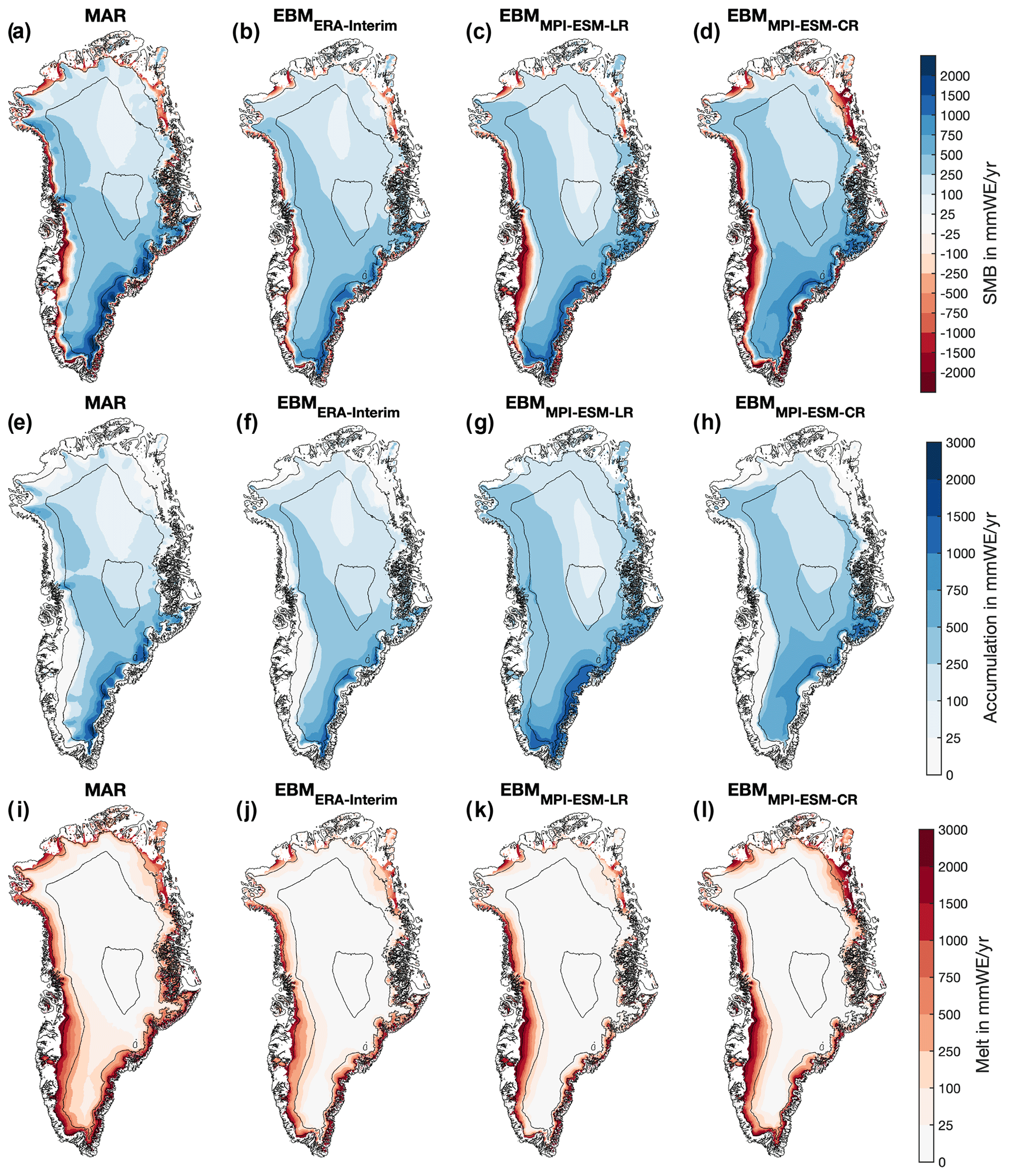
Figure 1 (a–d) SMB, (e–h) accumulation, and (i–l) melt from (a, e, i) MAR and EBM simulations forced with (b, f, j) ERA-Interim, (c, g, k) MPI-ESM-LR, and (d, h, l) MPI-ESM-CR for historical climate conditions. The values are averaged over 1980–2010. All variables are interpolated on the ISMIP6 topography and shown only for glaciated points. Note that accumulation is obtained as the residual of SMB minus melt as MAR does not provide accumulation as a direct output variable. Black contours mark surface elevations of 0, 1000, 2000, and 3000 m.

Table 3 Average and standard deviation of the annual SMB simulated with MAR and the EBM forced with ERA-Interim and a historical MPI-ESM simulation for the years 1980–2010. The annual SMB values are interpolated onto the ISMIP6 ice-sheet topography (see Sect. 2.4) except for RACMO^∗. The standard deviation reflects the interannual variability. Units are in gigatonne per annum (Gt a⁻¹). Accumulation is calculated as residual of the SMB and melt.

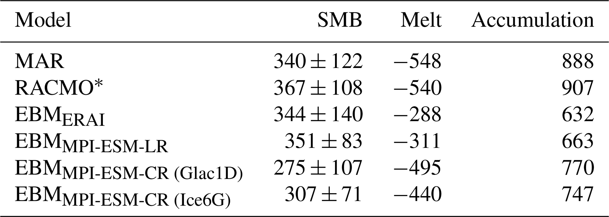
^∗ RACMO data are provided on a slightly different topography with 1 km horizontal resolution (see Noël et al., 2019, for details); the impact of the underlying topography
on the SMB values is expected to be small.

The SMBs from EBM_ERAI, EBM_MPI-ESM-LR, and EBM_MPI-ESM-CR show good agreement with SMBs from MAR for the historical period. The largest mass loss occurs along the low-elevation areas close to the coasts, with maxima in the west and southwest of Greenland. The largest mass gain is evident in the higher-elevation areas in the west and southeast of Greenland. For all simulations, the mass changes over northern central Greenland are small due to low precipitation at high elevations (see Fig. 2). Also, the gradients between areas of the most pronounced mass loss and gain are qualitatively similar in all simulations. Differences in the SMB fields are largest along the coasts in the southeast and west of the Greenland ice sheet. These differences are likely a result of the forcing data, model resolution (about 3.75^∘, approx. 250 km over Greenland for MPI-ESM-CR; 1.88^∘, approx. 120 km for MPI-ESM-LR; 0.75^∘, approx. 50 km for ERA-Interim; and 15 km for MAR), and underlying topographies (Fig. 2). Differences between MAR and EBM_ERAI are generally smaller than differences between MAR and EBM_MPI-ESM-CR or EBM_MPI-ESM-LR because ERA-Interim data were used as boundary forcing for the MAR simulation. Comparing SMBs derived from EBM_MPI-ESM-CR and EBM_MPI-ESM-LR shows that specifically the SMB differences in the north of the Greenland ice sheet, associated with more melt in EBM_MPI-ESM-CR along the coasts and enhanced accumulation in the center of the ice sheet compared to EBM_MPI-ESM-LR, are partly a consequence of the model resolution. In the following, we investigate the components that determine the SMB individually to better understand the mentioned differences between the simulations.

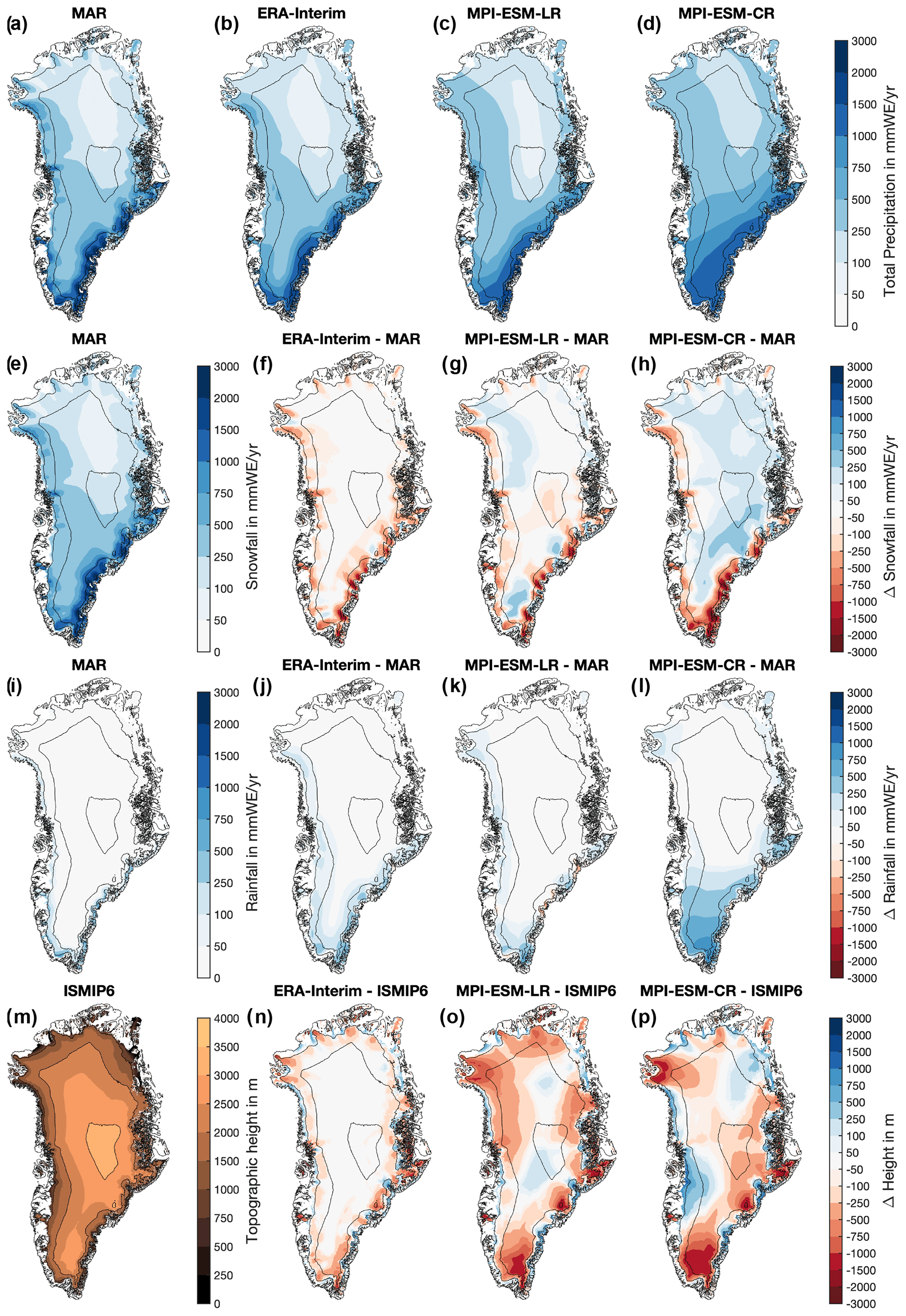
Figure 2 (a–d) Total Precipitation as simulated by (a) MAR, (b) ERA-Interim, (c) MPI-ESM-LR, and (d) MPI-ESM-CR for 1980–2010. (e–h) Snowfall and (i–l) rainfall in (e, i) MAR and differences between (f, j) ERA-Interim, (g, k) MPI-ESM-LR, and (h, l) MPI-ESM-CR and MAR. (m–p) Topography from (m) ISMIP6 and the differences in topography between ISMIP6 and (n) ERA-Interim, (o) MPI-ESM-CR, and (p) MPI-ESM-LR. Note that the values are bi-linearly interpolated onto the ISMIP6 topography from the original model data, not the downscaled values. Black contours mark surface elevations of 0, 1000, 2000, and 3000 m.

3.1 Accumulation

Accumulation patterns in MAR and the three EBM simulations are similar. However, they show some differences in the low-elevation areas in the southeast of the ice sheet and the northern plateau (Fig. 1). Integrated over the ice sheet, EBM_ERAI, EBM_MPI-ESM-CR, and EBM_MPI-ESM-LR simulate lower accumulation than MAR, as well as the Regional Atmospheric Climate Model (RACMO; Table 3; Noël et al., 2019). This difference is associated with less snowfall and more rainfall in ERA-Interim and the two MPI-ESM simulations than in the regional models, specifically in the low-elevation areas along the coastal areas of Greenland (Fig. 2). The underestimation of ERA-Interim's snowfall that extends into the high-elevation areas of the ice sheet is likely associated with an unrealistic representation of clouds and a low cloud bias, as well as shortcomings in modeling seasonal changes in surface temperatures (see Sect. 3.2; Miller et al., 2018). In the higher-elevation areas of most of the central parts of Greenland, MPI-ESM-CR and MPI-ESM-LR overestimate snowfall, which is tightly linked to topographic differences underlying the models, as well as model biases in the atmospheric circulation patterns affecting precipitation (Fig. 2; Mauritsen et al., 2019). Areas that are lower in MPI-ESM-CR and MPI-ESM-LR than MAR, mainly due to the spectral smoothing in MPI-ESM, generally show more snowfall in the MPI-ESM simulations (Fig. 2). Comparing the accumulation derived from EBM_MPI-ESM-CR with EBM_MPI-ESM-LR shows that accumulation patterns in the southeast of the ice sheet are more confined towards the east coast, but EBM_MPI-ESM-LR still presents a significant underestimation of accumulation in the low-elevation areas. Hence, even the higher resolution of MPI-ESM-LR is not sufficient to represent the regionally confined processes that determine the accumulation in these regions. The overestimation of accumulation in the north of the ice sheet is reduced in EBM_MPI-ESM-LR compared to EBM_MPI-ESM-CR. The reduction is likely associated with a better representation of the topographic gradients in the MPI-ESM-LR version of the model and an associated shift in precipitation patterns reducing precipitation at higher elevation. The comparison between EBM_MPI-ESM-LR and EBM_MPI-ESM-CR indicates that an increase in resolution should not always resolve all biases. This is in line with findings by van Kampenhout et al. (2019) showing that a regional grid refinement in simulations with the Community Earth System Model (CESM) did not improve all SMB components. Model biases, e.g., in the large-scale circulation, clouds, and precipitation patterns (Mauritsen et al., 2019), as well as uncertainties due to internal variability, are exhibited in all ESMs and explain part of the differences seen in the presented comparison.

Note that the EBM calculates snowfall as precipitation at temperatures below 0 ^∘C and partly compensates for these differences in snowfall and rainfall specifically along the coastal areas in the west and southeast of the ice sheet (not shown). The seasonal differences are larger. In summer, ERA-Interim simulates less snowfall and more rainfall but shows slightly less total precipitation than MAR, which impacts the melt patterns (not shown).

3.2 Melt

Integrated over the ice sheet, EBM_ERAI, EBM_MPI-ESM-CR, and EBM_MPI-ESM-LR simulate less melt than MAR and RACMO (Table 3), but the sign of the differences varies significantly depending on the region (Fig. 1). EBM_MPI-ESM-CR shows significantly more surface melt along the western margins of the ice sheet than MAR (Fig. 1). These areas are topographically higher in MPI-ESM-CR than the ISMIP6 topography (Fig. 2). One problem of downscaling melt in these regions is that temperatures are always at the freezing point during melting. By projecting the temperatures onto lower elevations, the height-corrected temperatures depart significantly from the freezing point towards higher temperatures. Hence, the vertical downscaling from higher elevations to low elevations overestimates melting. In contrast, the area in the south that is significantly higher than the ISMIP6 topography shows less melt. It indicates that most of the differences are closely related to differences in the topography. Comparisons with EBM_MPI-ESM-LR, which shows less melt in the north and west of the ice sheet compared to EBM_MPI-ESM-CR (Figs. 1 and 2), confirm that differences in the melt patterns are linked to the underlying topographies of the model versions. MPI-ESM-LR is slightly higher than MPI-ESM-CR and thereby closer to MAR on the northern and western flanks of the ice sheet; hence, EBM_MPI-ESM-LR shows less melt than EBM_MPI-ESM-CR in these areas. EBM_ERAI shows less melt in the southern and western parts of the ice sheets than MAR. These low melt rates are partly a result of the model tuning towards a similar integrated Greenland SMB value (see Table 3).

Heat fluxes towards the surface control predominately surface temperatures and melting. Miller et al. (2018), who compared surface energy fluxes over Greenland from different reanalyses with surface observations, found that ERA-Interim largely underestimates downward longwave and shortwave radiation, which is likely associated with an unrealistic representation of cloud optical properties. Low surface albedos in ERA-Interim and an associated underestimation of outgoing shortwave radiation partially compensate for the downward longwave radiation deficit. Further, seasonal biases in the latent heat fluxes dampen the seasonal changes in surface temperatures. Such biases are not unique to ERA-Interim but can also be found in other reanalyses (for details see Miller et al., 2018) and models, such as MAR (Fettweis et al., 2017). We find similar biases in the EBM_MPI-ESM-LR simulation which are likely associated with the simulated cloud cover.

4 SMB and ELA changes throughout the last deglaciation

The evaluation shows that major differences between MAR and EBM_MPI-ESM-CR are the increased melt on the western flank of Greenland and along the coastal areas, as well as the overestimation in accumulation in the southern part of Greenland. The latter can partly be reduced by increasing the model resolution, as shown by comparisons with EBM_MPI-ESM-LR. Given these model limitations, the SMB is modeled well in comparison to MAR (or other regional models; see also Fettweis et al., 2020) with the advantage of reduced computational costs that allow for a thorough investigation of the SMB for long-term climate simulations.

In the following, we present the climate of the deglaciation experiment with MPI-ESM-CR based on GLAC-1D boundary conditions. We limit the analysis to the Northern Hemisphere ice sheets only, with a specific focus on Greenland.

4.1 Greenland

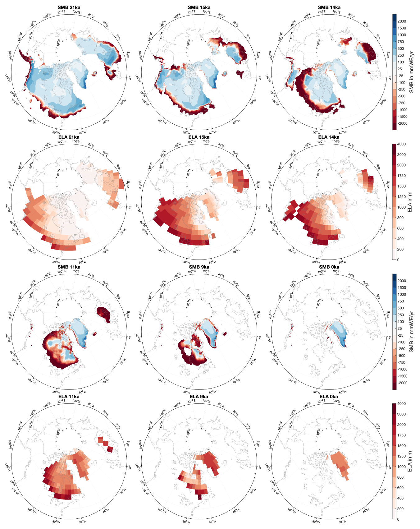
As the SMB is highly dependent on the prescribed ice-sheet geometry, it is challenging to interpret SMB changes for ice sheets that undergo substantial geometry changes throughout the deglaciation. As all Northern Hemisphere ice sheets except Greenland disappear entirely, we investigate the SMB evolution mainly for Greenland, where changes in the geometry were relatively small (Fig. 3, gray line in the top panel). Values for the SMB, ELA, accumulation, and melt integrated over Greenland are shown in Fig. 3. The SMB and ELA for six time slices of the deglaciation are shown in Fig. 4 in order to indicate the most drastic changes in the Northern Hemisphere ice-sheet configuration.

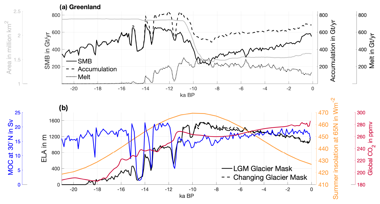
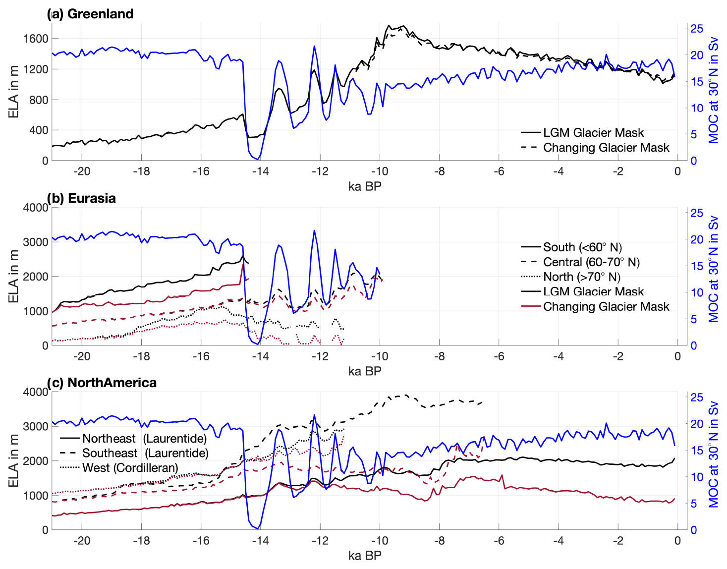
Figure 3 (a) Greenland SMB, accumulation, melt, and ice-sheet area and (b) equilibrium line altitude (ELA) and meridional overturning circulation (MOC) for the EBM_MPI-ESM-CR experiment, together with summer insolation at 65^∘ N and CO₂ concentration throughout the last deglaciation (21 to 0 ka). Here, 0 ka refers to the year 1950. SMB, accumulation, melt, and ELA (dashed) are integrated over the glacial mask of each individual 100-year time slice. Additionally, the ELA (solid) is integrated over the constant 21 ka ice-sheet mask in order to investigate differences due to the ice-sheet mask. The MOC is the overturning strength at 30.5^∘ N at a depth of 1023 m, as in Klockmann et al. (2016). The CO₂ concentration is taken from Köhler et al. (2017) and the summer insolation from Berger and Loutre (1991).

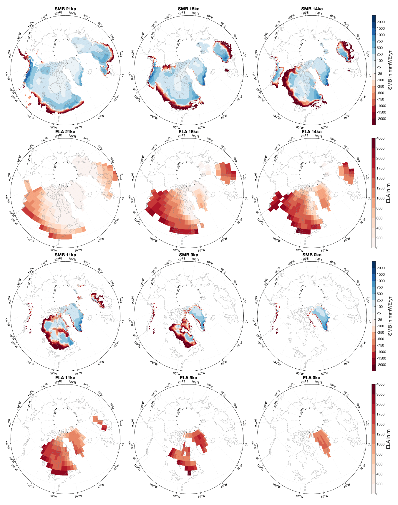
Figure 4 SMB and ELA for selected time slices (21, 15, 14, 11, 9 and 0 ka). Shown are the 100-year means. The SMB is interpolated on the GLAC-1D topography for each individual time slice and masked with the GLAC-1D glacier mask. The ELA, defined as elevation where the SMB equals zero, is calculated for each grid point on the native MPI-ESM-CR model grid from the 3-D SMB (see Sect. 2.1 and 2.3). The ELA is masked with the glacier mask used in the MPI-ESM-CR simulations.

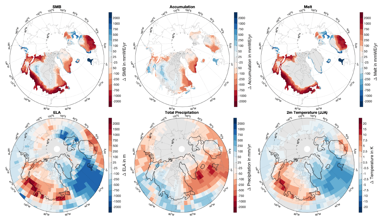
Cold Northern Hemisphere temperatures during the Last Glacial Maximum (LGM; approx. 21 to 19 ka) are associated with a positive Greenland-wide integrated SMB of about 380 Gt a⁻¹. This SMB is dominated by accumulation, while melt is close to zero (Figs. 3 and 4). This result is consistent with the Greenland ice sheet being close to its maximum extent during this period (Clark et al., 2009). Due to the increase in temperatures following an increase in Northern Hemisphere summer insolation by approximately 7 % of the LGM value and a simultaneous increase in the global CO₂ concentrations from 187 ppmv (parts per million by volume) at 19 ka to 228 ppmv at 15 ka, both accumulation and melt increase. The total accumulation over Greenland increases from about 420 Gt a⁻¹ at 19 ka to about 670 Gt a⁻¹ at 15 ka (more than 35 %). The largest accumulation increase is evident over the southwestern part of the ice sheets, which is associated with more precipitation (Fig. 5). Intriguingly, the increase in precipitation is not a uniform signal for the entire Northern Hemisphere but shows regional patterns, such as a decrease over parts of the North Atlantic and south of the Laurentide ice sheet edge. These patterns indicate that precipitation changes are not entirely thermodynamically driven (the atmosphere being able to hold more water with increasing temperatures) but points towards changes in the atmospheric dynamics. Melt increases from about 0 to 25 Gt a⁻¹ between the LGM and 15 ka. The growing melt is small and limited to the low-elevation areas along the coast of Greenland. This growth is a consequence of increasing summer temperatures that exceed the freezing point in these areas and lead to enhanced melt during summer. In the other areas over Greenland, temperatures are, despite warmer summers, still too cold to trigger melt. As the increase in accumulation dominates enhanced melting, the SMB time series increases until about 15 ka (Figs. 3 and 4). Interestingly, the ELA increases despite an SMB increase. Per definition, the ELA depends directly on shifts in areas of net melt and accumulation. Hence, it closely follows the increase in the ablation area. From the LGM to 15 ka, the area of net ablation increases from 0 to about 58 400 km².

Figure 5 Differences in SMB, accumulation and melt, precipitation, and 2 m temperatures, as well as 2 m summer temperatures, between 15 ka and the LGM. For the differences, SMB, accumulation, and melt are interpolated on the GLAC-1D topography of each individual time slice. The other variables are shown on the native MPI-ESM-CR model grid. Black contours in the lower panels indicate the ice-sheet mask at 15 ka.

A simultaneous increase in SMB and ELA seems to be counterintuitive at first given that in a present-day climate, a decrease in SMB over Greenland is associated with an increase in the ELA and vice versa (e.g., Le clec'h et al., 2019). As the climate warms, the area of net ablation expands, while the area of net accumulation recedes, which moves the ELA upward. As melt is close to zero in the glacial climate, the SMB is dominated by the significant growth of accumulation due to warmer atmospheric temperatures and the associated increase in precipitation. The dominance of the accumulation in controlling the SMB explains the counterintuitive behavior of the SMB and ELA in the glacial climate. Further, it suggests that changes in the ELA cannot be taken as a proxy for changes in the SMB.

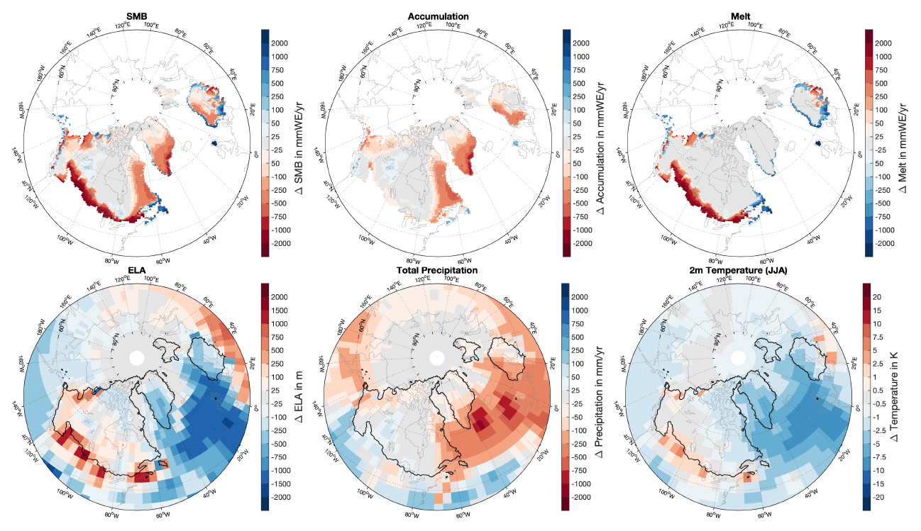
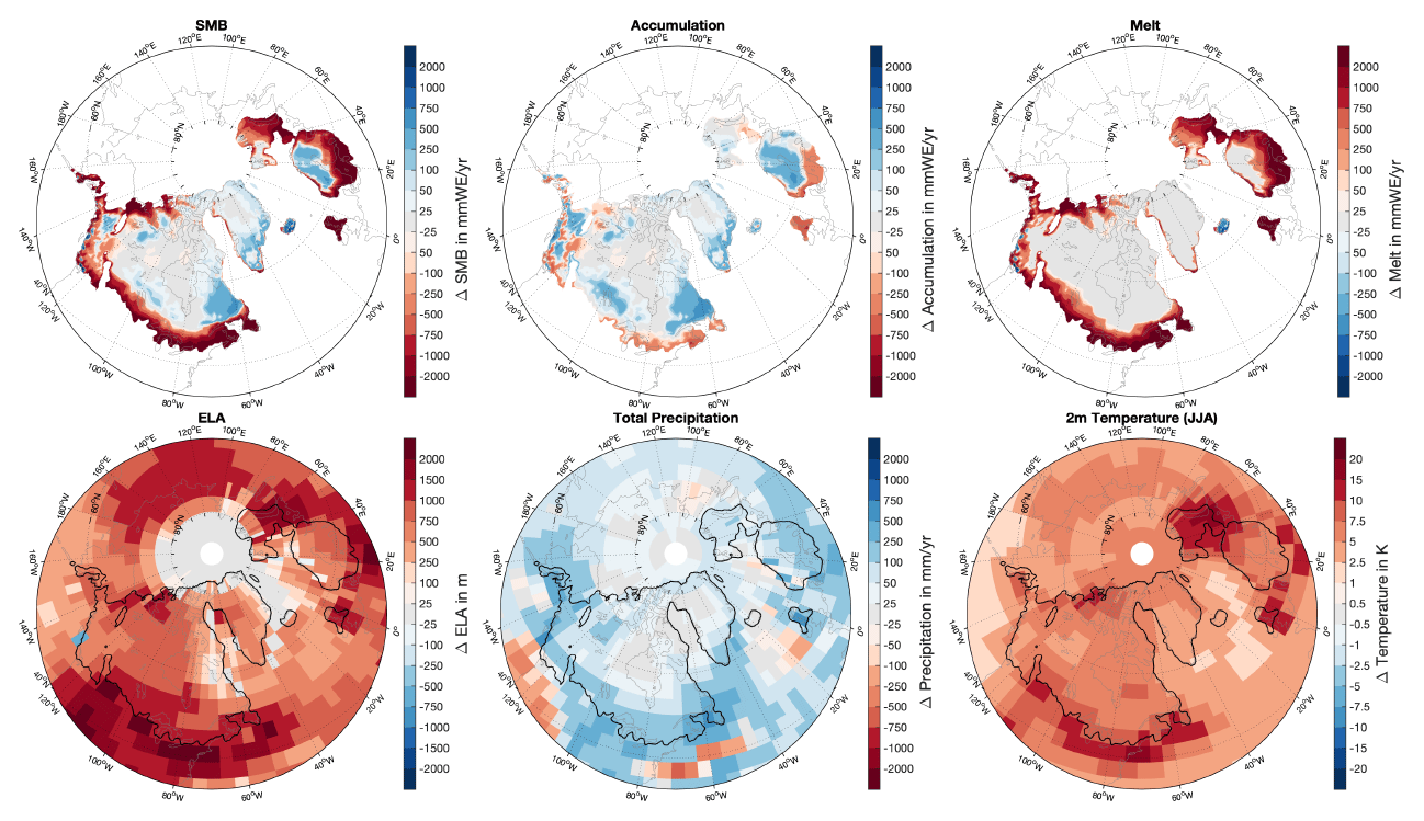
Figure 6 Similar to Fig. 5 but for differences between 14.6 and 15 ka.

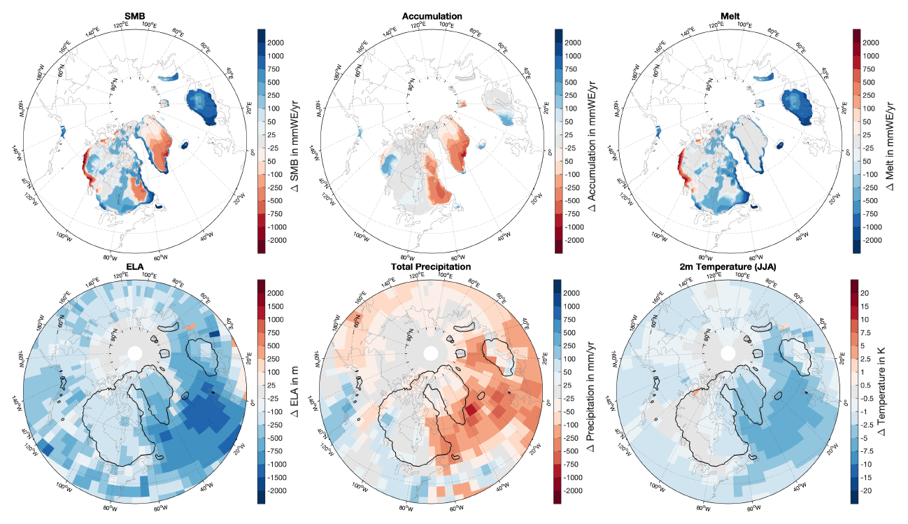
At around 14.6 ka, the SMB and ELA over Greenland decrease significantly for about 500 years, the SMB drops from about 630 to 380 Gt a⁻¹, and the ELA decreases from more than 460 to 120 m (Fig. 3). Regionally, differences are even larger (Fig. 6). These drastic changes are associated with a significant reduction in the AMOC as a response to increased inflow of freshwater from melting ice sheets into the global ocean, as prescribed from the GLAC-1D ice-sheet reconstructions. The strong meltwater pulse leads to a near shutdown of the thermohaline circulation and a significant cooling of the North Atlantic and adjacent regions (Fig. 6). Although the largest cooling is occurring over the North Atlantic, the annual cooling signal extends over large regions of the Northern Hemisphere, including the Arctic Ocean, the North Pacific, and large parts of Eurasia and North America (Fig. 6). Over Greenland, this cooling diminishes surface melt during summer, which is similar to LGM conditions. Again, the largest response is evident over the low-elevation areas along the southern coasts of Greenland (see also Fig. 5 for similarities). Associated with the overall cooling is a decline in precipitation which reduces accumulation by more than 40 % over the ice sheet. Although melt and accumulation again partly compensate for each other, accumulation changes occur over a much larger area and dominate changes in melt so that the integrated SMB decreases for Greenland (Fig. 3).

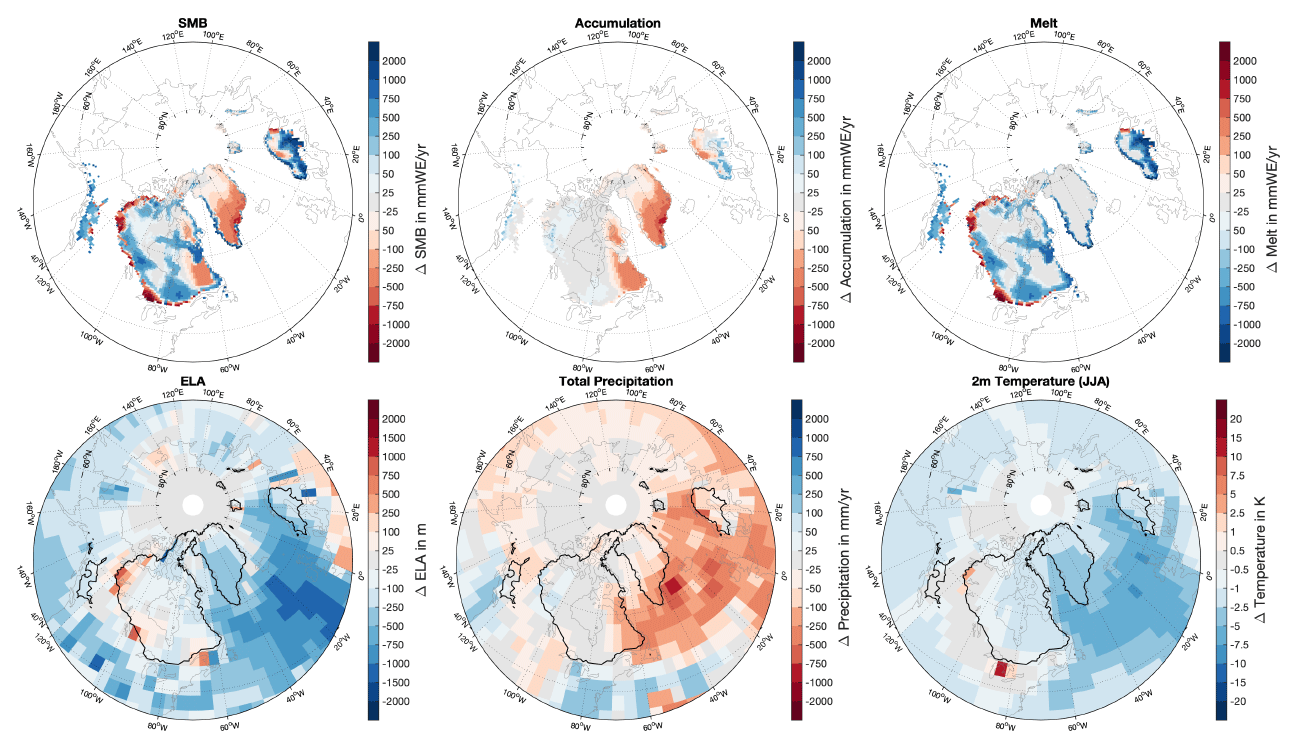
Figure 7 Similar to Fig. 5 but for differences between 11.6 and 12 ka.

After the recovery of the AMOC at around 14 ka, the SMB declines, and the ELA continues to move upward. It thereby follows the overall warming signal as a response to increasing insolation and atmospheric greenhouse gases (Figs. 3 and 4). The decline in the SMB is associated with an overcompensation of the accumulation by a significant increase in melting. Thus, ELA and SMB are anticorrelated from about 14 ka onward and continue to increase and decrease, respectively. Only at around 13.6 and 11.6 ka do the ELA and SMB decrease significantly again due to a second and third weakening of the AMOC. Similar to the first AMOC decline, the associated cooling of the North Atlantic and parts of Greenland leads to a decrease in accumulation, melt, and the ELA (Fig. 7). The changes are regionally very similar to the first event (Fig. 6). However, the Greenland integrated SMB shows a weaker signal in both cases than during the first freshwater event as the changes in accumulation and melt partly compensate for each other when integrated over the ice sheet (Fig. 3).

After the two AMOC events, the retreat of the Greenland ice sheet towards its present-day state continues and is associated with a decrease in SMB and an increase in ELA. The minimum SMB (216 Gt a⁻¹) is reached at 8.7 ka, and the maximum ELA (1556 m) occurs at 9.3 ka (Figs. 3 and 4), corresponding to the Holocene Thermal Maximum (for a recent review, see Axford et al., 2021). Due to the continuing deglaciation, Greenland experiences its largest ice volume and extent changes between 10.8 and 9.1 ka (the ice-sheet geometry influences SMB values during this period). At around 11.1 ka, the Northern Hemisphere summer insolation reaches its maximum and decreases continuously thereafter until the present, while the CO₂ concentration remains rather constant between 11.1 and 6 ka and slightly increases thereafter. Consequently, the ELA decreases, and the SMB begins to recover continuously after about 8.7 ka. Note that a series of smaller AMOC weakening events is evident at around 10.1, 8.4, and 7.1 ka, but their climate impact on the ELA and SMB does not manifest significantly in the time series for Greenland (Fig. 3). The ELA decrease and SMB increase continue until 200 years BP despite a slight increase in the CO₂ concentration. These continuing changes suggest that the decreasing summer insolation drives SMB and ELA changes between 9 ka and 200 years BP. It is not before 100 years BP that the ELA and SMB closely follow the CO₂ signal again. The sharp drop in the SMB and the uplift of the ELA for the last 100 years of the simulation is similar to the warm period observed in the coastal temperatures of Greenland in the 1930s (Chylek et al., 2006). At the end of the simulation, the ELA lies at about 1150 m, and the SMB reaches values of 550 Gt a⁻¹. These values are similar to values observed during the 21st century, although they are slightly higher as no anthropogenic forcings are considered in the deglaciation simulation (see Fig. 4, Sect. 3 and Table 3; Box, 2013).

The SMB and ELA derived from the MPI-ESM-CR simulation with the prescribed ICE-6G ice sheets are qualitatively similar to the presented results based on the GLAC-1D ice-sheet reconstructions (see Figs. A2 to A6). The overall trends of both variables, as well as the relationships between accumulation and melt (e.g., accumulation dominating melting until about 15 ka), are similar, but the timing of the weakening of the AMOC, as well as the magnitude, differs. These deviations are due to a different timing, magnitude, and location of meltwater release in the GLAC-1D and ICE-6G reconstructions, which are currently being investigated in a separate study (Kapsch et al., 2021).

4.2 Impact on the Eurasian and North American ELA

As discussed earlier, the North American (Laurentide and Cordilleran) and Eurasian (Fennoscandian, British Isles, and Barents–Kara Sea) ice sheets experienced substantial changes in their glacial extent throughout the last deglaciation (Fig. 4). Reconstructions suggest a steady retreat of the Eurasian ice sheets starting from the LGM until about 8.7 ka when the ice sheets converged to present-day conditions (e.g., Patton et al., 2017). The decline is highly discontinuous and shows an acceleration at around 17.8 ka. Similarly, the extent of the North American ice sheet started to decrease shortly after the LGM and continued until about 6.8 ka with only a little ice left at present (e.g., Carlson et al., 2007). As the SMB is highly dependent on the ice-sheet geometry, it is difficult to fully interpret SMB changes for the North American and Eurasian ice sheets. Hence, we only briefly point out the similarities between the climate responses of the ELAs over the North American, Eurasian, and Greenland ice sheets (see Figs. 5, 6, and 7) while keeping in mind that the interpretation is limited due to the extensive changes in the ice-sheet geometries throughout the deglaciation. To account for the massive ice-sheet changes in the time series, we split the ice sheets into different subregions and investigate their dependence on the ice-sheet geometry. Fig. 8 shows the ELA time series for Eurasia, subdivided into a southern (<60^∘ N), central (60–70^∘ N), and northern (>70^∘ N) ice sheet, and North America, split into a northern and southern Laurentide ice sheet (east of 120^∘ W and north of 60^∘ N and south of 60^∘ N, respectively) and a Cordilleran ice sheet (west of 120^∘ W).

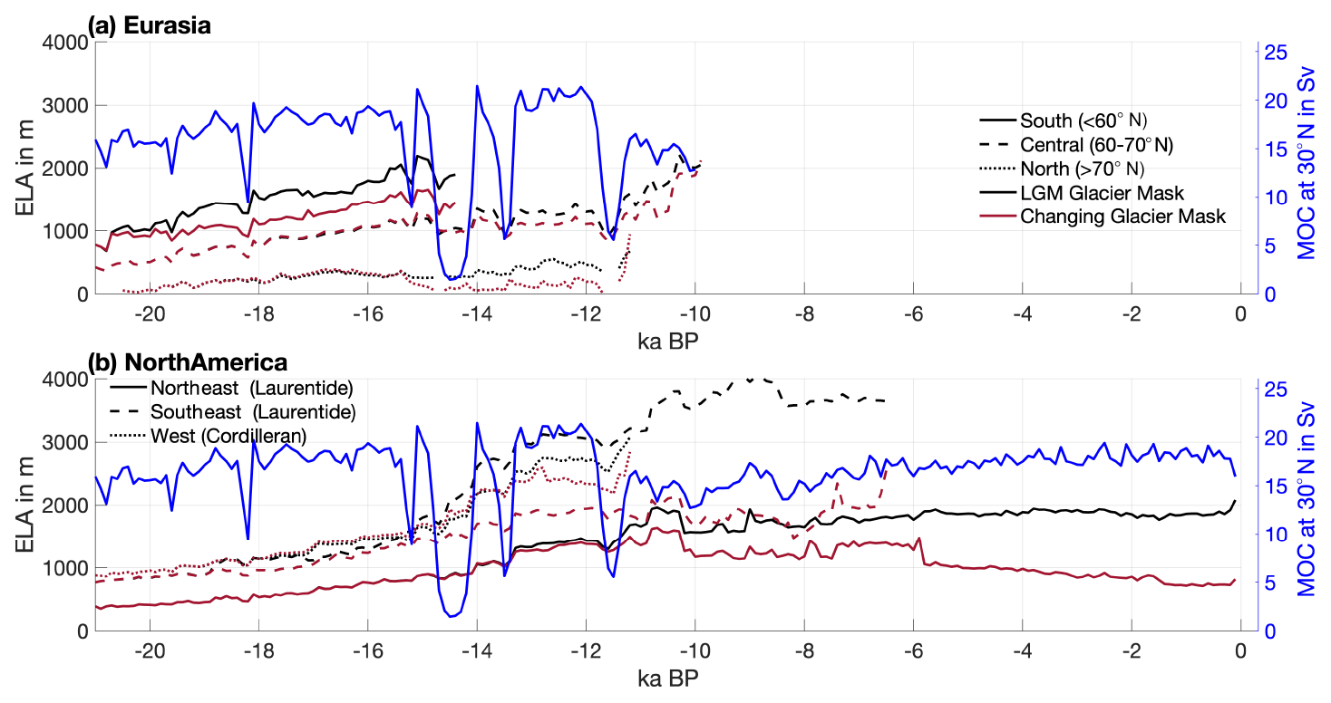
Figure 8 Similar to the bottom panel of Fig. 3 but for the subdivided (a) Eurasian and (b) North American ice sheets. The Eurasian ice sheet is subdivided into a southern (<60^∘ N), central (60–70^∘ N), and northern (>70^∘ N) part. The North American ice sheet is split into the northern and southern Laurentide ice sheet (east of 120^∘ W and north of 60^∘ N and south of 60^∘ N, respectively) and the Cordilleran ice sheet (west of 120^∘ W). The ELA is integrated for each region over the 21 ka ice-sheet mask (black) and over the ice-sheet mask of each respective time slice (red).

During the LGM, the average ELAs over Eurasia and North America are significantly higher than the ELA over Greenland for the same period except for the northeastern Laurentide and northern Eurasian ice sheets (see Figs. 4 and 8). Similar to the Greenland ice sheet, the ELA increases continuously until about 15 ka for the Eurasian and North American ice sheets. At around 14.5 ka, the southern and central Eurasian ice sheets both show a slight decrease in the ELA. This is likely associated with the AMOC slowdown (see Sect. 4.1); other AMOC events at around 19.6, 18.2, and 15.2 ka also result in a decrease in ELA for the southern and central Eurasian ice sheet. However, the signal in the ELA is relatively weak and regionally confined compared to the response over Greenland. Around 14.5 ka, the Eurasian ice sheet exhibits decreased ELAs on its western boundaries and the Laurentide ice sheet on its eastern boundaries since both melt and accumulation decrease in response to reduced North Atlantic temperatures (Fig. 6). This result suggests that the AMOC slowdown at 14.5 ka affected all ice sheets, at least regionally. Another possible contributing factor to the pronounced SMB and ELA variability over the Northern Hemisphere ice sheets during this time period are changes in the atmospheric circulation. Löfverström and Lora (2017) found that elevation changes in the North American ice sheets around the saddle collapse, defined by the separation of the Laurentide and Cordilleran ice sheets, caused significant changes in the stationary wave patterns. An amplifying factor for atmospheric circulation changes is the southward-extending sea-ice cover due to the AMOC slowdown and reduced North Atlantic sea-surface temperatures. Such changes have a significant influence on downstream precipitation and temperature patterns over the North Atlantic and adjacent areas.

After about 14 ka, the ELA continues to increase for nearly all ice sheets, following the overall warming signal. However, specifically for the southern ice sheets over Eurasia and North America, the changes in the ice-sheet extent have a large effect on the ELA. The signal in the ELA due to the changes in the ice-sheet mask exceeds the signal due to the natural climate variability in the ELA at around 20.6 ka for the southern Eurasian ice sheet, at about 18.9 ka for the northern Eurasian and southeast Laurentide ice sheets, at about 15.3 ka for the northern and central Eurasian ice sheets, and at 13.3 ka for the Cordilleran ice sheet (Fig. 8). Hence, the second and third AMOC slowdowns are only poorly reflected in the ELA time series, although similar regional responses are evident in Fig. 7. By 9.7 ka, Eurasia is completely ice free, while North America has only small ice sheets left (see Fig. 4).

5 Conclusions

In previous studies, changes and variability in the SMB have been analyzed mainly for the last century due to the availability of observations and the computational limitations of regional climate modeling. Here, we present the first analysis of SMB changes throughout the last deglaciation from a simulation with a comprehensive ESM. Despite the relatively low resolution of the MPI-ESM-CR simulation used as forcing for the EBM, the obtained SMBs for historical climate conditions show good agreement with SMBs derived from regional climate modeling (see Table 3). A comparison with SMBs derived from a simulation with the MPI-ESM-LR setup and ERA-Interim reanalysis reveals that discrepancies between the SMBs derived from MPI-ESM-CR and MAR are a result of the coarse resolution of the model (e.g., the extensive melt in the north of the Greenland ice sheet) and the quality of the forcing itself (e.g., precipitation patterns). In contrast to ERA-Interim, MPI-ESM evolves freely and does not assimilate any surface observations; hence, differences are to be expected. Further differences are related to underlying topographies of the native models, as well as the fact that most fluxes within the EBM are parameterized as they are not directly available from the model simulations in the required temporal resolution. For example, several studies have pointed towards the specific importance of the albedo parameterization for a realistic simulation of the surface mass balance (e.g., van Angelen et al., 2012). Here, we chose a parameterization that yields realistic SMBs for Greenland for the historical period (see Sect. 3). Given the computational advantages of the coarse-resolution version of MPI-ESM used in connection with the EBM for long-term simulations, these limitations and differences are an acceptable compromise.

Analyzing the MPI-ESM-CR deglaciation experiments for Greenland, we find that the SMB changes at the beginning of the deglaciation are associated with compensating effects of increasing accumulation and melt. The increase in accumulation dominates the increase in melt until about 14 ka as a significant melt is not evident before. After 14 ka, the SMB decreases, indicating that this time marks the onset of the deglaciation. The ELA begins to increase significantly earlier, from about 19 ka, suggesting that the deglaciation of Greenland might have been triggered earlier, likely by the insolation increase that set in before 21 ka. For Eurasia and North America, the ELA increases continuously from 21 ka, supporting such a hypothesis. An onset of the deglaciation over Greenland at around 14 ka is found in reconstructions and has been connected to the Bølling–Allerød warm period, which was associated with a strong AMOC and warm North Atlantic temperatures (e.g., Clark et al., 2002; Weaver et al., 2003). In MPI-ESM-CR, we do not find such warming but instead find an AMOC slowdown at 14.6 ka. This slowdown is caused by a meltwater pulse of more than 0.4 Sv, prescribed by the ice-sheet reconstructions (meltwater pulse 1A). As this meltwater pulse is associated with ice volume changes mostly in the North Atlantic and Arctic drainage basin in the ice-sheet reconstructions, it is assumed that the meltwater enters the North Atlantic and Arctic. This meltwater reduces the AMOC, which is associated with the strong cooling in the North Atlantic realm, in our model. The model does not simulate the strong melting needed for meltwater pulse 1A. After the end of the prescribed meltwater peak, the AMOC recovers in the model with some overshooting of the AMOC (peaking after 200–300 years BP). This result indicates that although our model does not simulate the Bølling–Allerød warm period as represented in proxy data, the overall progression of the deglaciation is represented reasonably well.

A comparison between ELAs and SMBs derived from MPI-ESM-CR simulations with different ice-sheet reconstructions (GLAC-1D and ICE-6G) as boundary forcing reveals that the results are qualitatively similar (see Figs. A2 to A6), although modeled changes in the AMOC are highly dependent on where the forcing is applied (e.g., Tarasov and Peltier, 2005). The comparison shows that the changes presented here are relatively robust, specifically for changes in the ELA. Exploring the differences in the model response due to prescribed ice-sheet reconstructions is the subject of a future study (Kapsch et al., 2021).

The AMOC slowdowns that occur throughout the last deglaciation are associated with significant changes in the ELA and SMB, specifically over Greenland and regionally also for the Eurasian and North American ice sheets. They are associated with cooling over the North Atlantic and a decrease in accumulation and melting in the adjacent regions. While the response in melt is directly affected by temperature changes, accumulation not only directly depends on temperature affecting the quantitative distribution of snow- and rainfall but also on other atmospheric properties, e.g., the capability of the atmosphere to hold water and changes in the atmospheric circulation and convection (Trenberth, 2011). The differences in the ELA in response to the AMOC slowdowns over the Laurentide and Eurasian ice sheets further away from the North Atlantic coasts are challenging to interpret for the following reasons. Substantial changes in the ice-sheet height and volume cause significant surface warming and enhance melting, specifically at the southern margins of the ice sheets (Figs. 7 and 6). Other contributing factors are more difficult to separate due to the nature of the experimental design, such as the effect of sea-level changes on the ice-sheet margins, feedbacks in response to changes in the sea level, sea ice, greenhouse gases, and ice-sheet height (see, e.g., Fyke et al., 2018). In addition, the missing ice-sheet dynamics might result in a modified ELA response due to differences in the ice-sheet height and configuration (Cronin, 2010).

Utilizing the SMB data set presented here as forcing for ice-sheet model simulations will allow for an investigation of ice-sheet dynamics during the last deglaciation. In the future, we plan to utilize the EBM in simulations with an interactive ice-sheet model, which is currently employed within the MPI-ESM setup in the scope of the project PalMod (Latif et al., 2016; Ziemen et al., 2019). The setup presented here is an important component of the fully coupled MPI climate–ice-sheet model system. Simulations with the full setup will allow us to investigate feedback processes between ice sheets and other climate components (see, e.g., Fyke et al., 2018,  for a recent review). It will also allow us to investigate processes and test hypotheses arising from the deglaciation simulations for other climates, such as, e.g., the last glacial inception, Marine Isotope Stage 3, and the future climate.

Appendix A: Supplementary figures

Table A1 Elevation classes used in the EBM.

Figure A1 Similar to Fig. 1 but for the MPI-ESM-CR_Ice6G simulation.

Figure A2 Similar to Fig. 4 but from the MPI-ESM-CR_Ice6G simulation.

Figure A3 Similar to Fig. 5 but for differences between 15 ka and LGM from MPI-ESM-CR_Ice6G.

Figure A4 Similar to Fig. A3 but for differences between 14.4 and 15 ka from MPI-ESM-CR_Ice6G. Note that a different time slice was chosen compared to Fig. 6 due to a later AMOC slowdown in MPI-ESM-CR_Ice6G compared to MPI-ESM-CR_Glac1D.

Figure A5 Similar to Fig. A3 but for differences between 11.2 and 12.2 ka from MPI-ESM-CR_Ice6G. Note that a different time slice was chosen compared to Fig. 7 due to different timings of the AMOC slowdown in MPI-ESM-CR_Ice6G compared to MPI-ESM-CR_Glac1D.

Figure A6 Similar to Figs. 3 and 8 but for EBM${}_{{\text{MPI-ESM-CR}}_{\mathrm{Ice}\mathrm{6}\mathrm{G}}}$ with prescribed ICE-6G reconstructions.