the Creative Commons Attribution 4.0 License.
the Creative Commons Attribution 4.0 License.
 | 07 Jan 2021
Drivers of Pine Island Glacier speed-up between 1996 and 2016
Ronja Reese
Fernando S. Paolo
G. Hilmar Gudmundsson
Pine Island Glacier in West Antarctica is among the fastest changing glaciers worldwide. Over the last 2 decades, the glacier has lost in excess of a trillion tons of ice, or the equivalent of 3 mm of sea level rise. The ongoing changes are thought to have been triggered by ocean-induced thinning of its floating ice shelf, grounding line retreat, and the associated reduction in buttressing forces. However, other drivers of change, such as large-scale calving and changes in ice rheology and basal slipperiness, could play a vital, yet unquantified, role in controlling the ongoing and future evolution of the glacier. In addition, recent studies have shown that mechanical properties of the bed are key to explaining the observed speed-up. Here we used a combination of the latest remote sensing datasets between 1996 and 2016, data assimilation tools, and numerical perturbation experiments to quantify the relative importance of all processes in driving the recent changes in Pine Island Glacier dynamics. We show that (1) calving and ice shelf thinning have caused a comparable reduction in ice shelf buttressing over the past 2 decades; that (2) simulated changes in ice flow over a viscously deforming bed are only compatible with observations if large and widespread changes in ice viscosity and/or basal slipperiness are taken into account; and that (3) a spatially varying, predominantly plastic bed rheology can closely reproduce observed changes in flow without marked variations in ice-internal and basal properties. Our results demonstrate that, in addition to its evolving ice thickness, calving processes and a heterogeneous bed rheology play a key role in the contemporary evolution of Pine Island Glacier.
- Article
(11308 KB) - Full-text XML
- BibTeX
- EndNote


Since the 1990s, satellite measurements have comprehensively documented the sustained acceleration in ice discharge across the grounding line of Pine Island Glacier (PIG, Fig. 1) in West Antarctica (Rignot et al., 2002; Rignot, 2008; Rignot et al., 2011; Mouginot et al., 2014; Gardner et al., 2018; Mouginot et al., 2019b). The changes in flow speed are an observable manifestation of the glacier’s dynamic response to both measurable perturbations, such as calving and ice shelf thinning, and poorly constrained variations in physical ice properties and basal sliding. Evidence from indirect observations has indicated that changes in ice shelf thickness have occurred since at least some decades before the 1970s (Jenkins et al., 2010; Smith et al., 2017; Shepherd et al., 2004; Pritchard et al., 2012). Within the last 2 decades, thinning of the grounded ice (Shepherd et al., 2001; Pritchard et al., 2009; Bamber and Dawson, 2020), intermittent retreat of the grounding line (Rignot et al., 2014), changes in calving front position (Arndt et al., 2018), and the partial loss of ice shelf integrity (Alley et al., 2019) have all been reported in considerable detail. At the same time, numerical simulations of ice flow have confirmed the strong link between ice shelf thinning, which reduces the buttressing forces, and the increased discharge across the grounding line (Schmeltz et al., 2002; Payne et al., 2004; Joughin et al., 2010; Seroussi et al., 2014; Favier et al., 2014; Arthern and Williams, 2017; Reese et al., 2018; Gudmundsson et al., 2019). Due to the dynamic connection between ocean-driven ice shelf melt rates and tropical climate variability (Steig et al., 2012; Dutrieux et al., 2014; Jenkins et al., 2016; Paolo et al., 2018), several model studies have focused on the important problem of simulating the response of PIG to a potential anthropogenic intensification of melt. Such external perturbations, in combination with ice-internal feedbacks including the marine ice sheet instability, can force PIG along an unstable and potentially irreversible trajectory of mass loss (Favier et al., 2014; Rosier et al., 2020). Whereas significant progress has been made in simulating the melt-driven retreat of PIG, less attention has been given to other processes that could affect the force balance and thereby inhibit or foster changes in ice dynamics. Increased damage in the shear margins of the ice shelf, for example, has been reported by Alley et al. (2019) and Lhermitte et al. (2020), and is known to reduce the buttressing capacity of an ice shelf (Sun et al., 2017). Moreover, a series of recent calving events has led to a sizeable reduction in the extent of the ice shelf and caused a potential loss of contact with pinning points along the eastern shear margin (Arndt et al., 2018).
The relative impact of changes in ice geometry, basal shear stress, and/or ice rheology on the dynamics of PIG has previously been emphasized in numerical studies by, for example, Schmeltz et al. (2002), Payne et al. (2004), Gillet-Chaulet et al. (2016), Joughin et al. (2019), and Brondex et al. (2019). In all cases, some combination of thickness changes, ice softening, a reduction in ice shelf buttressing, and variations in basal shear stress was required to attain an increase in flow speed comparable to observations. Similar conclusions were reached for other Antarctic glaciers. Based on a comprehensive series of model perturbation experiments, Vieli et al. (2007) suggested that the acceleration of the Larsen B Ice Shelf prior to its collapse in 2002 could not solely be explained by the retreat of the ice shelf front or ice shelf thinning, but required a further significant weakening of the shear margins. Complementary conclusions were reached by Khazendar et al. (2007), who demonstrated the important interdependence of the calving front geometry, a variable ice rheology, and flow acceleration based on data assimilation and model experiments for the Larsen B Ice Shelf.
In order to comprehensively diagnose the importance of all processes that have contributed to the acceleration of PIG over the period 1996 to 2016, this study brings together the latest observations and modelling techniques. We consider how calving, ice shelf thinning, the induced dynamic thinning upstream of the grounding line, and potential changes in ice-internal and basal properties have caused a different dynamic response across the ice shelf, the glacier's main trunk, the margins, and the tributaries. Initial observations indicated that the speed-up of PIG was primarily confined to its fast-flowing central trunk (Rignot et al., 2002; Rignot, 2008), though more complex spatio-temporal patterns of change have emerged more recently (Bamber and Dawson, 2020). The rapid and spatially diverse acceleration of the flow is an expression of the glacier's dynamic response to changes in the force balance, and it is imperative that numerical ice flow models are capable of reproducing this complex behaviour in response to the correct forcing. In general, the driving stress (τd), which depends on the ice thickness distribution, is balanced by resistive stresses, which include the basal drag (τb), side drag through horizontal shear (τW), longitudinal resistive forces (τL), and back forces by the ice shelf (τIS):
It is conceivable that each of the terms in Eq. (1) has changed considerably in recent decades in response to changes in calving front position, ice thickness, ice properties, and/or basal slipperiness. The interplay between different changing forces, in combination with the appropriate boundary conditions, underlies the observed speed-up of PIG (ΔU). Present-day observations of ΔU are generally assumed to be dominated by ice shelf thinning and induced dynamic loss and redistribution of mass upstream of the grounding line, which includes grounding line retreat and the associated loss of basal traction. Other possible contributions to ΔU, such as ice front retreat or changes in ice viscosity (including damage) or basal slipperiness, remain unquantified and are not generally included in model simulations of future ice flow at decadal to centennial timescales. These missing processes, if important, could lead to a systematic bias in model projections of future ice loss, or could prompt the use of unrealistically large perturbations in, for example, τIS in an attempt to reproduce observed values of ΔU.
In this study we used a regional configuration of the shallow ice stream (SSA) flow model Úa (Gudmundsson, 2020) for PIG to diagnose how individual processes (calving, ice thinning and associated grounding line movement, and changes in ice viscosity and basal slipperiness) have contributed to ΔU over the period 1996 to 2016. The diagnostic model response to prescribed changes in ice geometry was analysed, based on the latest observations of calving and ice thinning rates between 1996 and 2016. For each perturbation, changes in the stress balance (Eq. 1) and the associated ice flow response were computed. Any further discrepancies between modelled and observed changes in velocity were attributed to variations in ice properties, commonly parameterized by a rate factor A, and changes in basal slipperiness C. Results enabled us to validate the ability of current-generation ice flow models to reproduce the complex response of PIG to a range of realistic forcings, and to verify whether common model assumptions such as a static calving front and fixed ice viscosity and basal slipperiness are indeed justified.
Although the aforementioned method provides insights into the individual contribution of geometrical perturbations and changes in ice viscosity and basal slipperiness to overall changes in ice flow, results will likely depend on a number of structural assumptions within the ice flow model. Previous studies have shown that different forms of the sliding law, for example, can produce a distinctly different simulated response of PIG to changes in ice thickness (Joughin et al., 2010; Gillet-Chaulet et al., 2016; Joughin et al., 2019; Brondex et al., 2019). Joughin et al. (2010, 2019) showed that a regularized Coulomb law or the plastic limit of a non-linear viscous power law provides a better fit between modelled and observed changes in surface velocity along the central flow line of PIG compared to a commonly used Weertman law with a cubic dependency of the sliding velocity on the basal shear stress. Motivated by the above considerations, we explore new ways to derive spatially variable constraints on the form of the sliding law and thereby provide the first comprehensive, spatially distributed map of basal rheology beneath PIG.
The remainder of this paper is organized as follows. In Sect. 2.1 we introduce the observational datasets used to constrain and validate the ice flow model. Additional details about our data processing methods are provided in Appendix A. Section 2.2 outlines the experimental design and provides a summary of the main model components. Further technical details about the model set-up and a discussion about the sensitivity of our results to numerical model details are provided in Appendix B and Appendix D respectively. Results and an accompanying discussion of all experiments are provided in Sect. 3.1–3.3. Final conclusions are formulated in Sect. 4.
The first aim of this study is to simulate the dynamic response of PIG to a series of well-defined geometric perturbations over the period 1996 to 2016 and compare model output to observed changes in surface speed over the same time period. As detailed in Sect. 1, geometric perturbations are considered to be observed changes in the calving front position and observed changes in ice thickness of the ice shelf and grounded ice. We are primarily interested in the relative contribution of each perturbation to the observed speed-up of PIG between 1996 and 2016. Each contribution can be characterized by a relative change in velocity, , where U96 and U16 were obtained from model optimization experiments, as described in Sect. 2.2.1, and velocities of the perturbed states (Upert) were obtained from a series of diagnostic model calculations, as described in Sect. 2.2.2. First, the data sources required for each of these experiments are listed.
2.1 Observed changes of Pine Island Glacier between 1996 and 2016
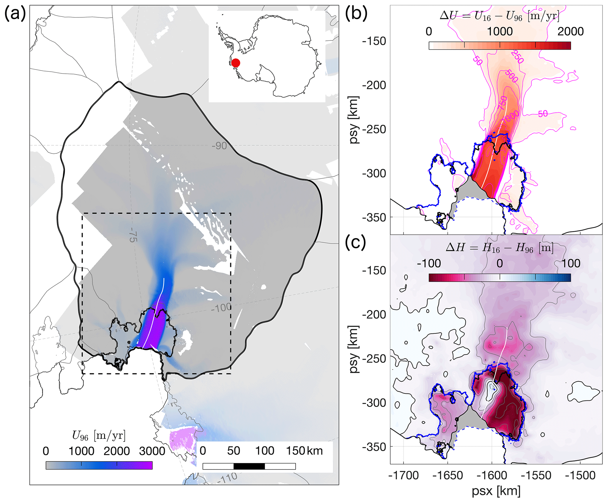
Figure 1Pine Island Glacier (PIG) and its location in West Antarctica. (a) Surface speed of PIG in 1996 in m yr−1, as reported by the MEaSUREs programme (Mouginot et al., 2019a). Solid black outlines delineate the extent of the PIG catchment (Rignot et al., 2011) and 1996 grounding line position (Rignot et al., 2014). The white line along the central flow line indicates the location of the transect in Fig. 2. The dashed rectangle corresponds to the extent of panels (b) and (c). (b) Observed increase in surface speed (Mouginot et al. (2019a), colours and contours in m yr−1 and loss of ice shelf extent (grey shaded area) between 1996 and 2016. The blue line indicates the 2011 grounding line (Rignot et al., 2014). (c) Total change in ice thickness between 1996 and 2016 (ΔH in m), based on a combination of CPOM data (Shepherd et al., 2016) for the grounded ice and newly analysed data for the ice shelf (Appendix A). The zero contour is shown in black; other contours in grey are spaced at 20 m intervals.
Our study area and model domain encompasses the 135 000 km2 grounded catchment (Rignot et al., 2011) and seaward-floating extension of PIG in West Antarctica, as depicted in Fig. 1a. To investigate the physical processes that forced the contemporary speed-up of the glacier and its increase in grounding line flux between the years 1996 and 2016, we needed detailed observations of the surface velocity, ice thickness, and calving front position for both years.
The surface velocity measurements used in this study were taken from the MEaSUREs database (Mouginot et al., 2019a, b). For 1996, synthetic-aperture radar data from the ERS-1 and ERS-2 missions were processed using interferometry techniques and combined into a mosaic with an effective timestamp of 1 January 1996. The MEaSUREs velocities for 2016 were based on feature tracking of Landsat 8 imagery with an effective timestamp of 1 January 2016. The change in surface speed between the two years is shown in Fig. 1b, and we refer to, for example, Rignot et al. (2014) and Gardner et al. (2018) for a more comprehensive description of these observations.
To obtain an accurate estimate of the ice thickness distribution of PIG in 1996, we compiled a time series of surface height changes from a comprehensive set of overlapping satellite altimeter data between 1996 and 2016. The integrated altimeter trend over the 20-year time interval, shown in Fig. 1c, was subtracted from the recent BedMachine Antarctica reference thickness (Morlighem et al., 2020). As satellite altimeters are very precise instruments capable of detecting small changes in surface elevation, our approach is more robust compared to thickness estimates based on a snapshot digital elevation model, such as the ERS-1-derived product (Bamber and Bindschadler, 1997), which has poor vertical accuracy. The BedMachine Antarctica reference thickness is based on the high-resolution Reference Elevation Model of Antarctica (REMA; Howat et al., 2019), tied to CryoSat-2 data, and an improved estimate of bedrock topography using mass conservation methods. The nominal date of the BedMachine geometry corresponds to the date stamp of the REMA elevation model, which is spatially variable but largely between 2014 and 2018 for PIG. We denote the 1996 and BedMachine Antarctica ice thickness estimates as H96 and H16 respectively, where , with ΔH the integrated altimeter trend. Estimates of ΔH were based on a combination of existing Centre for Polar Observation and Modelling (CPOM) measurements of surface elevation changes for areas upstream of the 2016 grounding line (Shepherd et al., 2016) and newly analysed data for the floating ice shelf. A detailed description of our methods and a map of the data coverage for ΔH can be found in Appendix A and Fig. A1 respectively.
The grounding line location for H16 (blue line in Fig. 1b–c) corresponds to the DInSAR-derived grounding line in 2011 from Rignot et al. (2014), since this is included as a constraint in the generation of the BedMachine Antarctica bed topography (Morlighem et al., 2020). The grounding line for approximately follows the 1992–1996 DInSAR estimates (Rignot et al., 2014), as shown in Fig. A1. To further improve the agreement between the model and DInSAR grounding line in 1996, some localized adjustments less than 150 m were made to the bed topography. The final grounding line location for H96 is depicted in Fig. 1a–c.
Alongside the above-listed observed changes in flow dynamics and ice thickness, the calving front of PIG retreated by up to 30 km between 1996 and 2016 during a succession of large-scale calving events; see, for example, Arndt et al. (2018). We traced the calving front positions in 1996 and 2016 from cloud-free Landsat 5 and Landsat 8 panchromatic band images with timestamps of 18 February 1997 and 25 December 2016 respectively. Both outlines are included in Fig. 1b–c, and the ice shelf area that was lost between 1996 and 2016 is shaded in grey.
2.2 Experimental design
2.2.1 Optimization experiments
To obtain an optimal model configuration for the state of PIG in 1996, we explicitly solved the stress balance by assimilating the estimated ice thickness (H96), measured calving front position, and measured surface velocities in the shallow ice stream model Úa (Gudmundsson et al., 2012; Gudmundsson, 2020). An analogous routine was applied for 2016. This “data assimilation” or “optimization” step is commonly adopted in glaciology (see MacAyeal, 1992, for one of the earliest examples) to minimize the misfit between modelled and observed surface velocities through the optimization of uncertain physical parameters. The optimization capabilities of Úa (further details are provided in Appendix B) were used to optimize the uncertain spatial distribution of the rate factor, A, and basal slipperiness, C. These physical parameters define the constitutive model and the relationship between basal shear stress τb and basal sliding velocity Ub respectively:
Glen's law, Eq. (2), relates the strain rates to the deviatoric stress tensor τ. A creep exponent n=3 was used throughout this study. Equation (3) is known as a Weertman sliding law (Weertman, 1957) and describes a linear viscous, non-linear viscous, or close-to-plastic bed rheology for m=1, m>1, and m≫1 respectively. Throughout this study, a range of values for m are considered, as specified below. For each m we performed a new inversion for A and C; example results for m=3 are provided in Appendix B. The outcome of the optimization step is an estimate for A and C that best fits the stress balance in Eq. (1) for given observations of geometry and surface velocity, associated measurement errors, and assumptions about the prior values of A and C. Solutions for A and C are not generally unique but rather depend on the choice of optimization scheme and several poorly constrained optimization parameters. Further details about the optimization scheme used and a discussion about the robustness of our results with respect to uncertain optimization parameters are provided in Appendix B and D.
2.2.2 Geometric perturbation experiments
The optimal model configuration in 1996 was subsequently used as the reference state for a series of numerical perturbation experiments, aimed at simulating the impact of observed changes in geometry on the flow of PIG. For each perturbation, the modified force balance (Eq. 1) and corresponding perturbed velocities were diagnosed within Úa. The rate factor and basal slipperiness were kept fixed to their 1996 values, although the basal traction was reduced to zero and slipperiness values became irrelevant in areas that ungrounded due to ice thinning. Experiments will be referred to as , with a variable subscript to indicate the type of perturbation and a superscript to specify the value of the sliding exponent m.
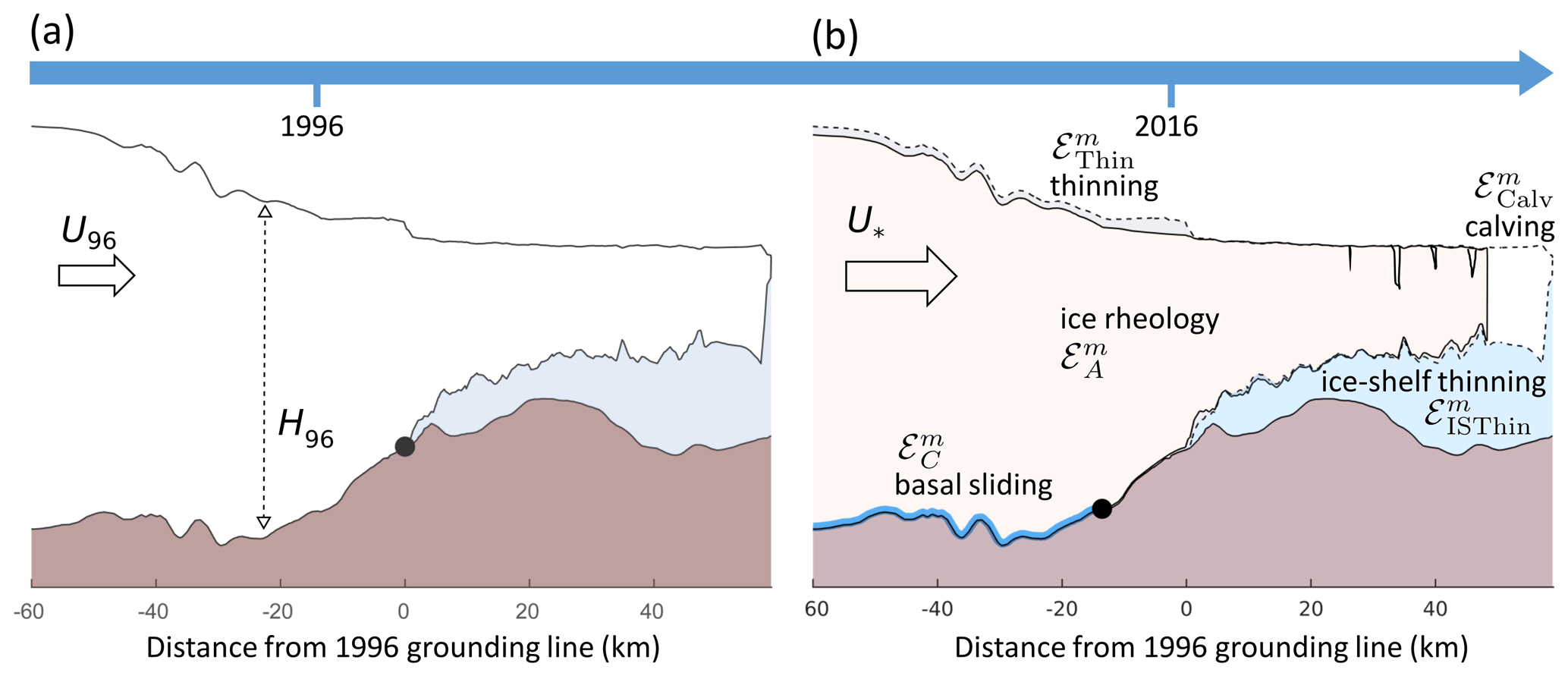
Figure 2Overview of changes along the Pine Island Glacier centreline from (a) year 1996 to (b) year 2016. Increased ice flow is driven by a combination of calving, ice shelf thinning, and dynamic thinning with movement of the grounding line, as well as changes in basal sliding and ice rheology. Transects of the geometry are based on observations along the flow line indicated in Fig. 1; black dots indicate the respective grounding line positions in both years. Crevasses are introduced for illustration purposes only and do not strictly correspond to observed features. The importance of each “driver of change” was investigated in a series of numerical perturbation experiments, denoted by in panel (b), with m indicating the sliding exponent and * the respective experiment described in Sect. 2.2.
-
. Changes in the calving front location were prescribed to reflect the loss of ice shelf between 1996 and 2016 (see Fig. 1b–c). All model grid elements downstream of the 2016 calving front (grey shaded area in Fig. 1b) were deactivated, whilst elements upstream of the 2016 calving front remained fixed to avoid numerical interpolation errors. All other model variables were kept fixed. The difference between the 1996 surface velocity and the perturbed velocity will be denoted by .
-
. Changes in ice shelf thickness were prescribed, corresponding to observed thinning of the ice shelf between 1996 and 2016 (Fig. 1c). Note that the calving front and grounding line location did not change in this experiment, which is similar to previous studies by, for example, Reese et al. (2018) and Gudmundsson et al. (2019). The instantaneous change in surface velocity due to ice shelf thinning will be denoted by .
-
. Observed changes in both the floating and grounded parts of PIG were prescribed. This caused the grounding line to move from its 1996 position (black line in Fig. 1b–c) to the 2016 position (blue line in Fig. 1b–c). Velocity changes caused by thinning of the floating and grounded ice will be denoted by .
-
. Combined changes in calving front position (as in ) and thinning (as in ) were prescribed. Corresponding velocity changes will be denoted by .
A schematic overview of the experiments is provided in Fig. 2. While allows us to assess the instantaneous impact of calving between 1996 and 2016, the experiments simulate the instantaneous response to total changes in ice shelf thickness between 1996 and 2016. The separate perturbations make it possible to disentangle changes in ice shelf buttressing caused by each process, and hence their relative importance for driving the transient evolution of the flow. However, both experiments ignore the time-dependent, dynamic response of the upstream grounded ice and the associated loss of basal traction due to grounding line movement. Dynamic thinning of grounded ice, as well as migration of the grounding line, is included in the experiments , which allows us to determine the full dynamic response to changes in ice thickness. Finally, the experiments combine both calving and ice thinning, and thereby accounts for all geometric perturbations.
2.2.3 Estimates of changes in A and C
Later on we show that geometric perturbations alone are not able to fully reproduce the observed patterns of speed-up across the PIG catchment. It is conceivable that, along with the evolving geometry, variations in ice and basal properties have contributed to the changes in flow between 1996 and 2016. Indeed, feedback mechanisms are likely to cause an important interdependence between geometry-induced changes in ice flow, shear softening, and/or changes in basal shear stress. Reliable observations of changes in rheology and basal properties are not available, but numerical optimization simulations can provide valuable insights into their evolution. We used the inverse method as described in Sect. 2.2.1 and Appendix B to estimate necessary bounds on the magnitude and spatial distribution of changes in A and C that are required, beside the geometrical changes already applied, to produce the speed-up of PIG between 1996 and 2016. Changes in A and C are treated separately.
-
. The aim of these experiments is to determine possible changes in the rate factor between 1996 (A96) and 2016 (A16). A96 was previously obtained in part 1 (optimization step) of the experimental design. To estimate A16, an inverse optimization problem was solved for the 2016 PIG geometry (H16) and velocities (U16), but using a cost function that was minimized with respect to A only. The slipperiness C was kept fixed to its 1996 solution.
-
. These experiments are analogous to , but the cost function in the inverse problem was optimized with respect to C only, whereas the rate factor A was kept fixed to its 1996 solution.
3.1 Ice dynamic response to changes in geometry between 1996 and 2016
We present results for the first set of perturbation experiments, which simulate the impact of observed changes in geometry on the flow of PIG. As detailed in Sect. 2.2.2, perturbations are split between four separate cases: (1) calving (); (2) thinning of the ice shelf (); (3) thinning of the ice shelf and grounded ice (), which includes associated movement of the grounding line and changes in basal traction; and (4) the combined impact of all the above (). We did not previously specify the value of the sliding exponent; however, here we set m=3, which is a commonly adopted value in ice flow modelling and describes a non-linear viscous (or Weertman) bed rheology. Results for different values of m will be explored in Sect. 3.3.
Results for the relative change in surface speed, , for each of the above perturbations are presented in Fig. 3a–d. In addition to spatial maps of relative velocity changes, we present flux calculations for two gates perpendicular to the flow within the central part of PIG, as displayed in Fig. 3a. Gate 1 is situated about 50 km upstream of the 2016 grounding line and captures the inland propagation of changes in ice flow. Gate 2 approximately coincides with the 2016 grounding line position and captures changes in grounding line flux, which is a direct measure for PIG's increasing contribution to sea level rise and an important indicator of change.
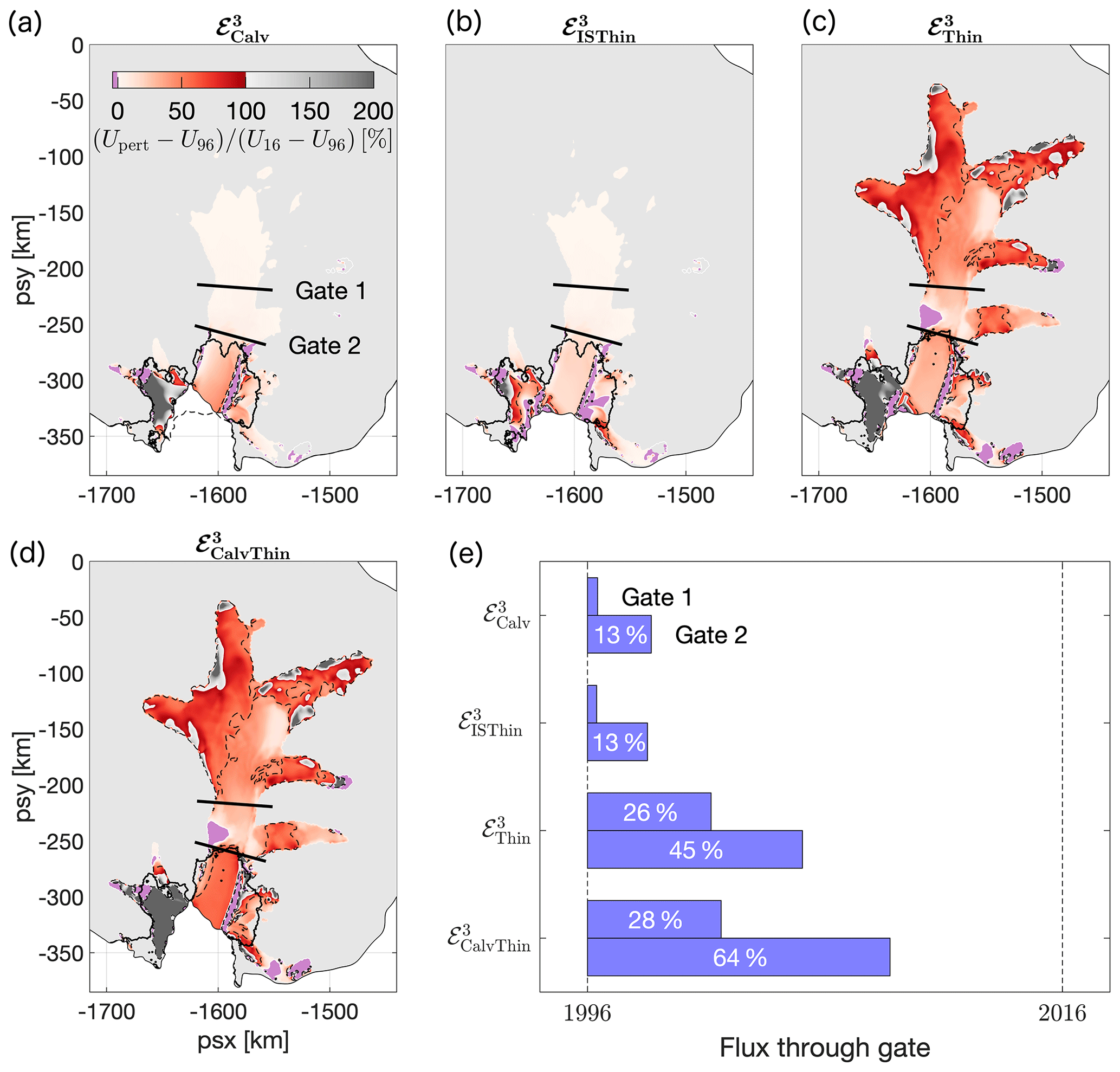
Figure 3Modelled changes in surface speed compared to 1996 for prescribed perturbations of the Pine Island Glacier geometry. (a) Retreat of the calving front. (b) Thinning of the ice shelf. (c) Thinning of the ice shelf and grounded ice, including grounding line retreat. (d) Calving and thinning combined. For each perturbation, the modelled change in speed (Upert−U96) is expressed as a percentage of the observed speed-up between 1996 and 2016 (U16−U96). Dashed black lines correspond to the 50 % contour. Panel (e) shows the percentage of the observed flux changes through Gate 1 and 2 that can be explained by the respective perturbations. The simulated impact of calving and thinning in experiment only represents 28 and 64 % of the measured flux changes respectively. Possible explanations for the unaccounted-for increase in flow speed are provided in Sect. 3.2 and 3.3 .
Calving as simulated in causes changes in flow speed that are predominantly restricted to the outer ice shelf, where it accounts for up to 50 % of the observed speed-up between 1996 and 2016 (Fig. 3a). A smaller dynamical impact is also felt upstream of the grounding line, caused by the calving-induced reduction in ice shelf buttressing and mechanical coupling between the floating and grounded ice. Along the fast-flowing central trunk of PIG, calving typically accounts for less than 10 % of the observed speed-up, with little or no effect on the dynamics of the upstream tributaries. Our results are consistent with earlier work by Schmeltz et al. (2002), in particular their calving scenario “part 2”. The only area with negative relative changes in our simulation is the western shear margin of the ice shelf, where modelled and observed changes in flow speed have the opposite sign. Extensive damage, a process that is not captured by this experiment, has caused this margin to migrate, and significant interannual variations in flow speed have been reported by Christianson et al. (2016). Figure 3e shows that calving accounts for 2 and 13 % of the observed flux changes through Gate 1 and 2 respectively, which confirms the minor instantaneous changes to the flow upstream of the grounding line.
Thinning of the ice shelf as simulated in experiment induces a flow response that is similar to calving, as shown in Fig. 3b, and indicates that calving and ice shelf thinning have caused a comparable perturbation in the buttressing forces. The largest percentage changes are found on the ice shelf and are typically less than 25 %, while the relative flux changes through Gate 1 and 2 are identical to the calving experiment (Fig. 3e). Ice shelf thinning is generally accepted to be the main driver of ongoing mass loss of PIG, and patterns of ice shelf thinning elsewhere in Antarctica are strongly correlated to observed changes in grounding line flux (Reese et al., 2018; Gudmundsson et al., 2019). However, the force perturbations that result from ice shelf thinning alone, in particular the instantaneous reduction in back forces τIS, are not sufficient to reproduce the magnitude of observed changes in upstream flow, consistent with previous studies (Seroussi et al., 2014; Joughin et al., 2010, 2019). Indeed, experiment demonstrates that the direct and instantaneous contribution of ice shelf thinning to observed changes in grounding line flux is less than 25 %. Instead, time-evolving changes in geometry and mass redistribution upstream of the grounding line, which may cause grounding line retreat and associated loss of basal traction, play a significant role in increasing the dynamic response of the glacier. These dynamic changes, caused indirectly by changes in the calving front position and ice shelf thinning, were not captured by the experiments and but are considered in experiment .
In experiment we prescribed the time-integrated change in ice thickness between 1996 and 2016 for both the floating ice shelf and upstream grounded ice. This perturbation incorporates the observed recession of the PIG grounding line between 1996 and 2016. The combined reduction in ice shelf buttressing, loss of basal friction due to grounding line retreat, and changes in driving stress caused a significant and far-reaching impact on the flow, as displayed in Fig. 3c. Modelled changes on the ice shelf are consistent with and similar in amplitude to . Upstream of the grounding line, modelled changes relative to observations are between 25 and 50 % along the central trunk and up to 100 % along the tributaries. In addition, results demonstrate that glacier-wide changes in ice thickness account for 26 and 45 % of the observed changes in ice flux through Gate 1 and 2 respectively (Fig. 3e).
In the final perturbation experiment, , the combined effect of calving and changes in ice thickness was simulated. Modelled versus observed changes in surface speed are shown in Fig. 3d. The spatial pattern is consistent with previous experiments, and the amplitude of the response is approximately equal to the added response of experiments and , i.e. . The corresponding percentage changes in ice flux through Gate 1 and 2 are 28 and 64 % respectively, whereas modelled changes in flow across the actual grounding line account for about 75 % of the observed increase in flux between the years 1996 and 2016. Although this experiment prescribes all observed changes in PIG geometry over the observational period, model simulations are unable to capture a significant percentage of the observed speed-up. This is most noticeable along the fast-flowing central trunk upstream of the grounding line, whereas discrepancies decrease along the slow-flowing tributaries in the high catchment. We also note that, in one area between Gate 1 and 2, modelled and observed changes in surface speed have opposite signs.
Although it is not unexpected to find differences between diagnostic model output and observations, the consistently suppressed response of the model to realistic perturbations in ice geometry is indicative of a structural shortcoming within our experimental design. Indeed, results show that, for a non-linear viscous bed rheology described by a Weertman sliding law with constant sliding coefficient m=3, changes in ice geometry alone cannot account for the complex and spatially variable pattern of speed-up over the observational period, i.e. . In the remainder of this study, two possible hypotheses are analysed that enable the gap to be closed between geometry-induced changes in ice flow and the observed speed-up of PIG. The first hypothesis, which is considered in Sect. 3.2, assumes that bed deformation can indeed be described by a non-linear viscous power law with m=3, but further temporal variations in ice viscosity and/or basal slipperiness are required in addition to changes in geometry: . The second, alternative hypotheses, discussed in Sect. 3.3, assumes that internal properties of the ice and bed have not significantly changed between the years 1996 and 2016, i.e. ΔUA≈0 and ΔUC≈0, but a different physical description of the basal rheology is required instead.
3.2 Changes in the rate factor and basal slipperiness between 1996 and 2016
In transient model simulations of large ice masses such as Antarctica's glaciers and ice streams, it is common to assume that the advection of A with the ice, or changes due to temperature variations and fracture as well as changes in basal slipperiness C, exerts a second-order control on changes in ice flow. As such, temporal variability in A and C is often ignored, based on the assumption that these changes are sufficiently slow and do not significantly affect the flow on typical decadal to centennial timescales under consideration. The aim of experiments and , as outlined in Sect. 2.2.3, is to establish whether this is a valid assumption, or whether previously ignored changes in A and/or C can provide a realistic explanation for the discrepancy between simulated and observed changes in the surface speed of PIG in the geometric experiment . Experiment assumes that, in addition to changes in geometry, temporal variations in A alone are able to account for the significant increase in flux that was unaccounted for in previous experiments. Alternatively, assumes that, in addition to changes in geometry, temporal variations in C alone are able to resolve the discrepancy in Sect. 3.1 between the modelled and observed speed-up. In line with previous experiments we assume a Weertman sliding law with m=3. The results for both experiments are summarized in Fig. 4.
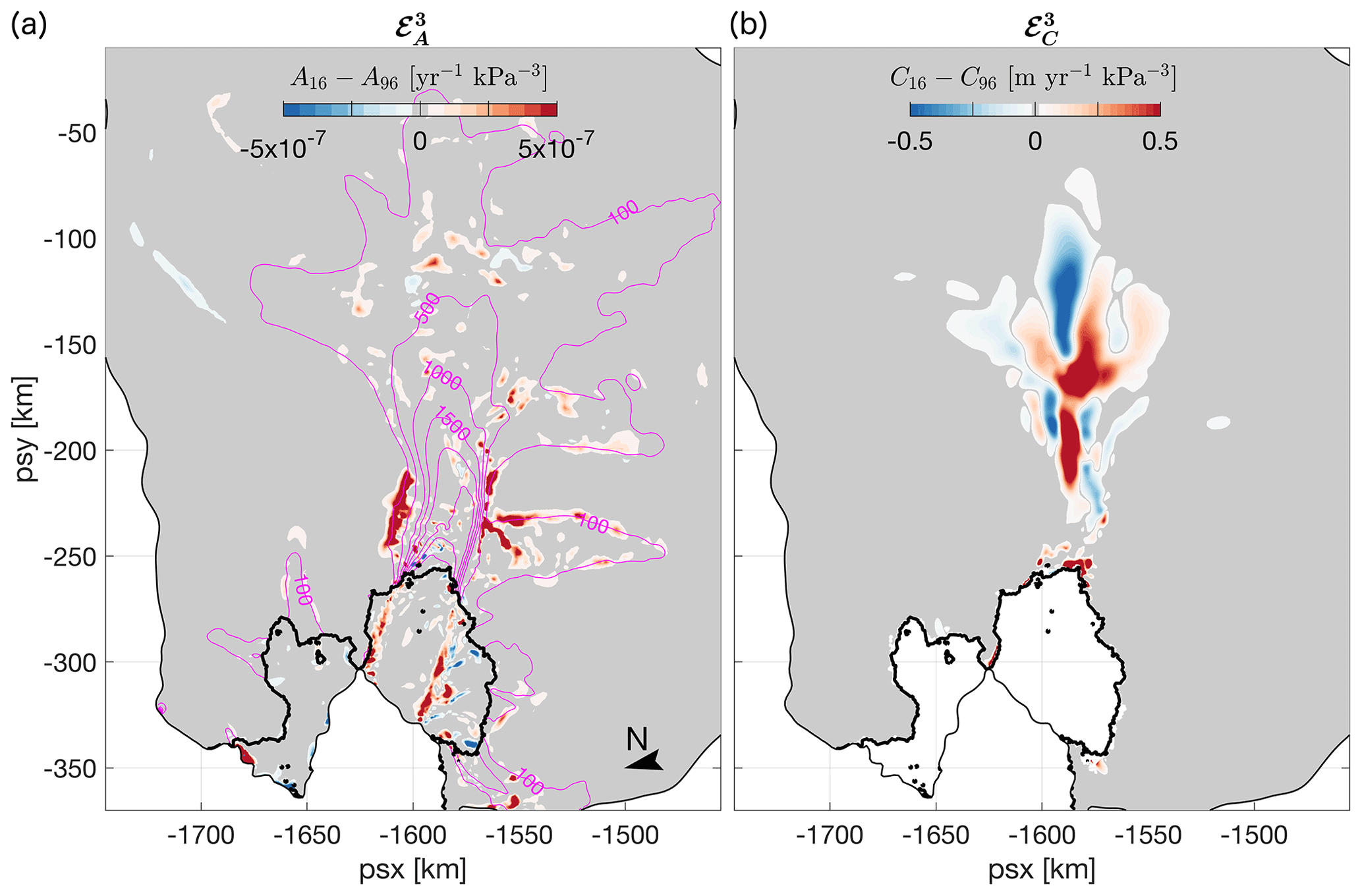
Figure 4(a) Results for the experiment: changes in the rate factor A required to fully reproduce observed changes in surface speed of the ice shelf and grounded ice between the years 1996 and 2016. The sliding exponent m=3 and basal slipperiness C were kept fixed for grounded areas. Magenta contours (in m yr−1) correspond to the surface speed in 2016. (b) Results for the experiment: changes in the basal slipperiness C required to reproduce the observed increase in surface speed of the grounded ice between 1996 and 2016. The rate factor A is assumed constant between 1996 and 2016.
Changes in A (Fig. 4a) needed to fully reproduce the speed-up of PIG between the years 1996 and 2016 are spatially coherent and predominantly positive. This suggests a reduction in ice viscosity between 1996 and 2016, as a result of localized heating, enhanced damage within the ice column, or changes in anisotropy. The largest changes are found in distinct geographical areas: a localized increase within the shear margins of the ice shelf and a more widespread increase along the slower-moving flanks (magenta contours in Fig. 4a indicate surface speed in 2016) of the main glacier and westernmost tributary, about 20 km upstream of the 2016 grounding line. Changes within the ice shelf shear margins are consistent with their increasingly complex and damaged morphology, as is apparent from satellite images (Alley et al., 2019). Weakening of the ice in these areas is sufficient to account for the remaining 50 % of observed changes in ice shelf speed-up that could not previously be reproduced by calving and ice shelf thinning alone (experiment ). Projected changes in A along the flanks of the upstream glacier, on the other hand, are more ambiguous. Values in excess of 10−7 yr−1 kPa−3 correspond to an equivalent increase in “ice” temperature by up to 40 ∘C. This is nonphysical unless (part of) the change is attributed to damage or evolution of the ice fabric. Based on our analysis of Sentinel and Landsat satellite images, there is no obvious indication of recent changes in the surface morphology in these areas. Either significant and widespread changes in the thermal and mechanical properties have occurred beneath the surface or the observed speed-up and thinning in these areas, as previously reported by Bamber and Dawson (2020), cannot be convincingly attributed to changes in the rate factor.
Alternatively, temporal changes in C can be invoked to reproduce the discrepancies between modelled and observed changes in surface speed between the years 1996 and 2016. Results presented in Fig. 4b suggest that a complex and widespread pattern of changes in the slipperiness is required across an extensive portion of PIG's central basin and its upper catchment. Despite the complex and poorly understood relationship between C and quantifiable physical properties of the ice–bed interface, it is difficult to understand how any single process or combination of physical processes could be responsible for the large and widespread changes in C over a time period of 2 decades. Further information, such as a time series of maps similar to Fig. 4b, can potentially be used to test the robustness of this result and provide further insights into the physical processes that could control such changes. This is the subject of future research.
We note that, in the experiment, velocities on the floating ice shelf were largely unaffected by changes in C and remained significantly slower than observations (not shown). In contrast, changes in the rate factor were able to fully account for the speed-up of the ice shelf. On the other hand, large variations in A were needed to reproduce the changes in ice dynamics along the slow-moving flanks of PIG (Fig. 4a), whereas only small changes in C less than 10−3 yr−1 kPa−3 m were required to explain this behaviour. It is therefore conceivable that, in addition to PIG's evolving geometry, an intricate combination of changes in both the rate factor and basal slipperiness are required to reproduce the glacier's complex and spatially diverse patterns of speed-up over the last 2 decades. It is however not straightforward to disentangle these processes in the current modelling framework.
3.3 Evidence for a heterogeneous bed rheology
The relationship between changes in geometry and the dynamic response of a glacier crucially depends on the mechanical properties of the underlying bed and subglacial hydrology. So far, we have assumed that basal sliding can be represented by a non-linear viscous power law with spatially uniform stress exponent m=3 (see Eq. 3). A power-law rheology is particularly suitable for the description of hard-bedded sliding without cavitation (Weertman, 1957), but missing processes such as variations in effective pressure or the deformation of a subglacial till layer with a maximum shear (yield) stress could be important limitations. Some evidence has been provided for plastic bed properties underneath ice streams either from observations (Tulaczyk et al., 2000; Minchew et al., 2016) or from laboratory experiments (Zoet and Iverson, 2020). Most recently, Gillet-Chaulet et al. (2016), Brondex et al. (2019), and Joughin et al. (2019) used numerical simulations to show that different sliding laws can cause a distinctly different dynamical response of PIG to changes in geometry, and observed changes in surface velocity were best reproduced for sliding exponents m≫1 or using a hybrid law that combines power law with Coulomb sliding. Although the results are compatible with a plastic bed underlying the central trunk of PIG, no constraints on the spatial variability in basal rheology were derived.
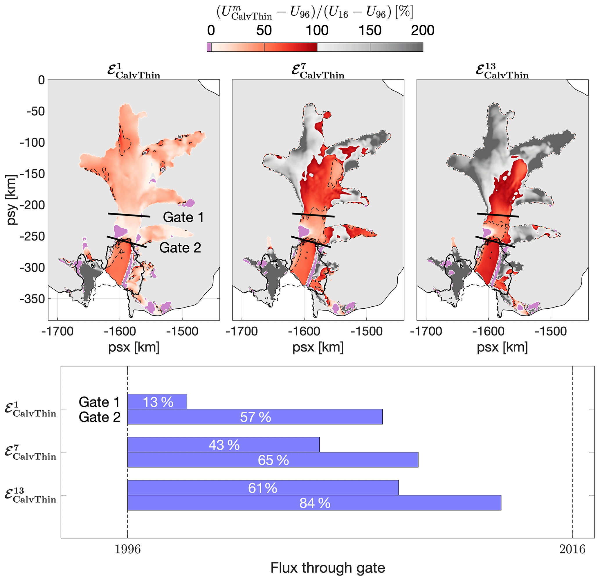
Figure 5Dependency of simulated-versus-observed changes in surface speed on the sliding-law exponent: (a) m=1, (b) m=7, and (c) m=13. Dashed black lines correspond to the 50 % contour. Larger values of m cause an increased response of the modelled surface speed to geometrical changes (calving, thinning, and grounding line retreat). For m>3, the modelled response of slow-flowing ice in the upstream catchment exceeds observed changes by more than a factor of 2, whereas for m=13 modelled changes of the fast-flowing central trunk are still smaller than observed changes. (d) Changes in flux through Gate 1 and 2 as a percentage of observed changes for m=1, 7, and 13.
In order to quantify how different values of the sliding exponent affect the sensitivity of PIG to changes in geometry across the catchment, we repeated perturbation experiments for a range of sliding-law exponents, from m=1 to m=21 at increments of 2. Results for m=1, 7, and 13 are shown in Fig. 5. A linear rheology induces a simulated response to calving and thinning that accounts for less than 50 % of the observed changes everywhere. For m=7, relative changes in flow speed exceed 100 % along significant portions of the slower-flowing tributaries. For m=13, which effectively corresponds to a plastic rheology, the modelled response overshoots observations by more than 100 % in most areas, except along the main glacier, where the response approaches 100 %. Across the model domain, a significant positive correlation exists between m and relative velocity changes, indicating a stronger dynamic response to perturbations in geometry with increasing values of m. This finding is in agreement with Gillet-Chaulet et al. (2016) and Joughin et al. (2019); however our maps show that no single, spatially uniform value of the sliding exponent is able to produce a good match between model output and observations across the entire catchment.
The positive correlation between the flow response and m is an inherent property of the adopted physical description of glacier dynamics. For the shallow ice stream approximation with a non-linear viscous sliding law, the first-order response of the surface velocity, δU, to small perturbations in surface elevation, δS, was previously determined by Gudmundsson (2008) and depends on m in the following non-linear way:
The transfer amplitude contains complicated positive functions f1 and f2 that generally depend on the wavelength of the surface perturbation, geometrical factors such as the local bed slope, and the basal slipperiness C. Further details are provided in Appendix C. Despite the simplifying assumptions that underlie the analytical expression of obtained by Gudmundsson (2008), results from our simulations , indicate that Eq. (4) is also applicable to the more complex setting of PIG. Indeed, as explained in detail in Appendix C, we found that across a large portion of the PIG catchment the transfer amplitude provides a suitable model to describe the dependency of the relative velocity changes on m. The parameters f1 and f2 were treated as spatially variable fields, and best estimates and were obtained as a solution of the minimization problem
The non-linear dependency of on m can then be approximated by
Using this dependency of the simulated velocity changes on m, one can derive an “optimal” spatial distribution of the sliding exponent, moptimal(x), such that everywhere, namely
By construction, the variable sliding exponent moptimal(x) enables reproducing 100 % of the observed speed-up of PIG in response to calving and ice thickness changes. The results, depicted in Fig. 6a, indicate that plastic bed conditions (m≫1) prevail across most of the fast-flowing central valley and parts of the upstream tributaries. Values generally increase towards the grounding line, whilst linear or weakly non-linear bed conditions are consistently found in the slow-flowing inter-tributary areas. This finding is compatible with the presence of a weak, water-saturated till beneath fast-flowing areas of PIG and a hard bedrock or consolidated till between tributaries (Joughin et al., 2009). The transition to lower exponents in areas with slower flow (<600 m a−1) is also consistent with results based on a Coulomb-limited sliding law, which produces Coulomb plastic behaviour at speeds >300 m a−1 and weakly non-linear viscous sliding at slower speeds (Joughin et al., 2019).
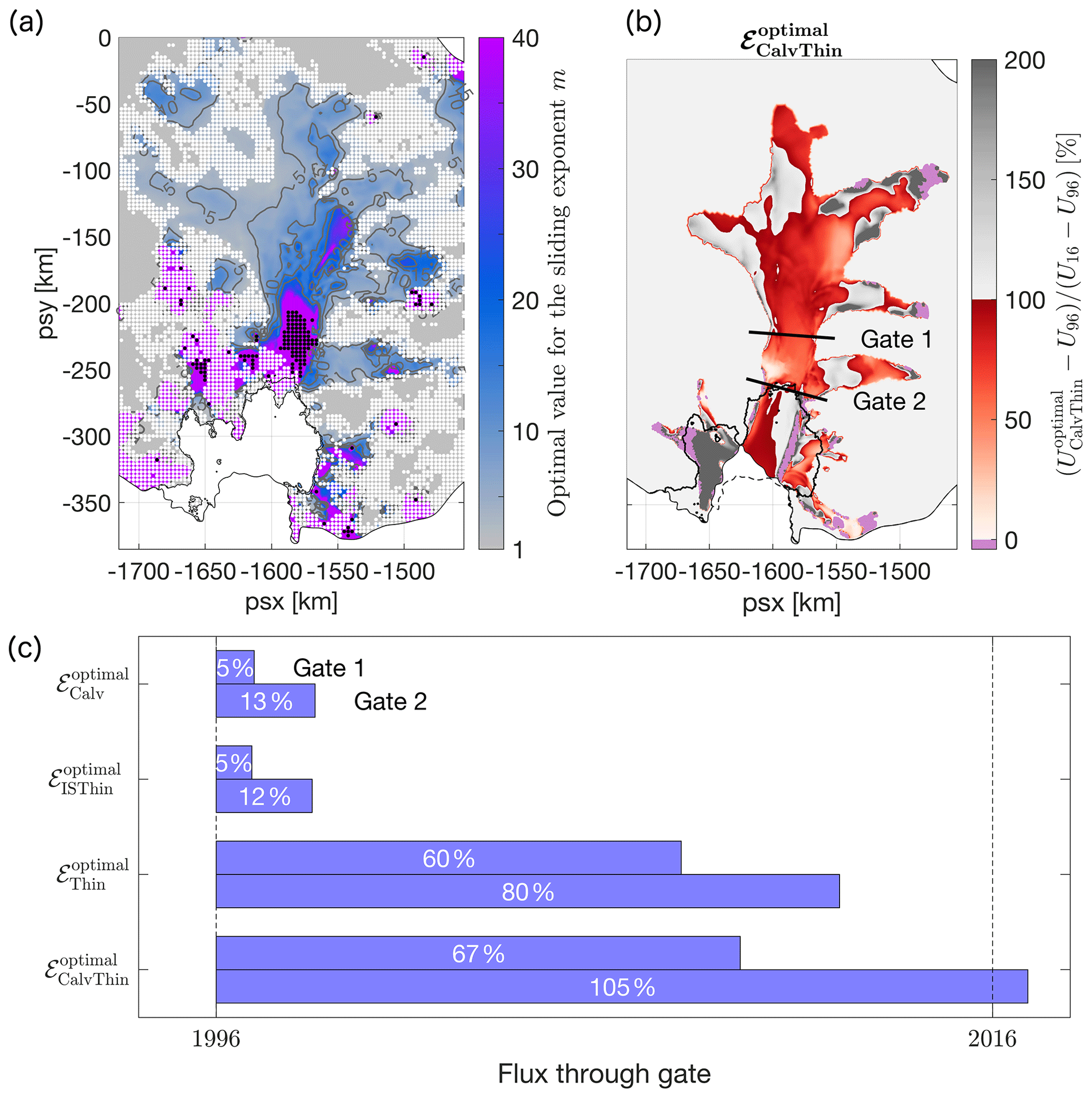
Figure 6(a) Optimal values of the sliding exponent, required to ensure close agreement between modelled and observed changes in flow velocity of Pine Island Glacier between the years 1996 and 2016. White and black dots mark areas where such an agreement cannot be achieved for different reasons: white dots indicate a poor fit between the transfer function and , with R2<0.9; black dots indicate areas where a positive, finite solution for moptimal in Eq. (7) does not exist and non-linear viscous sliding cannot reproduce observed changes in surface flow. (b) Same as Fig. 3d but for optimal values of the sliding-law exponent in panel (a). (c) Same as Fig. 3e but for optimal values of the sliding-law exponent in panel (a).
Two interesting properties of the regression model in Eq. (4) are worth noting. Firstly, for m→∞, the function approaches a horizontal asymptote with limit equal to f1. As a consequence, the associated solution for moptimal diverges to ∞ for locations x where and becomes negative where . In these areas, indicated by black dots in Fig. 6a, no non-negative, finite value of m exists such that , and conventional Weertman sliding is unable to fully reproduce the observed flow changes in response to thickness changes and calving. Either a different form of the sliding law is required or additional changes in the rate factor A and/or basal slipperiness C are needed. These findings are the subject of a forthcoming study. Our second observation concerns locations where U16 or U96 contains significant measurement uncertainties, or where no discernible changes in the surface velocity were measured, i.e. . In these areas, the non-linear regression was generally found to be poor, with R2 values smaller than 0.9 as indicated by the white dots in Fig. 6a. As no reliable estimate for moptimal could be obtained for areas shaded in white or black in Fig. 6a, values were instead based on a nearest-neighbour interpolation.
It is important to reiterate that the regression method used crucially relies on non-trivial measurements of changes in surface velocity () and cannot be used to retrieve information about the basal rheology of ice bodies that are presently in steady state. It should also be noted that values of and were derived independently for each node of the computational mesh, whereas the continuum mechanical properties of glacier flow would suggest a non-zero spatial covariance and . The optimal solution for m is therefore not automatically mesh independent or robust with respect to the amount of regularization in the inversion. This concern is discussed further in Appendix D.
In order to demonstrate the improved model response to thinning and calving for a spatially variable sliding exponent moptimal(x), we performed a new inversion with moptimal(x) and subsequently repeated the geometric perturbation experiments . The results are presented in Fig. 6b and c. Compared to spatially uniform values of m (Fig. 3d and Fig. 5), a spatially variable basal rheology generally improves the fit between observed changes in flow and the modelled response across the entire basin. Based on the flux changes through Gate 1 and 2, we find that (1) calving and ice thickness changes in combination with a spatially variable, predominantly plastic bed rheology account for 67 and 105 % of flux changes through Gate 1 and 2 respectively, compared to 28 and 64 % for a uniform non-linear viscous sliding law with exponent m=3; that (2) calving and ice shelf thinning caused an almost identical response in ice dynamics upstream of the grounding line; and that (3) dynamic thinning and grounding line movement account for most of the flux changes between the years 1996 and 2016. The remaining mismatch between the observed and modelled response in Fig. 6b can, at least in part, be attributed to uncertainties in moptimal(x). This is of particular relevance in the vicinity of the grounding line and for parts of the central trunk, where the non-linear regression method in Eq. (4) did not provide a reliable or finite estimate for moptimal. Previous studies, for example by Gillet-Chaulet et al. (2016) and Joughin et al. (2019), have demonstrated a better agreement between modelled and observed speed-up using Coulomb-limited sliding laws, such as those proposed by Budd et al. (1984), Schoof (2006), and Tsai et al. (2015). Our results are consistent with these earlier studies and suggest that power-law sliding does not adequately capture the physical relationship between basal shear stress and sliding in the vicinity of the grounding line.
Based on the most comprehensive observations of ice shelf and grounded ice thickness changes to date, and a suite of diagnostic model experiments with the contemporary flow model Úa, we have analysed the relative importance of ice shelf thinning, calving, and grounding line retreat for the speed-up of Pine Island Glacier over the period 1996 to 2016. The detailed comparison between simulated and observed changes in flow speed has provided insights into the ability of a modern-day ice flow model to reproduce dynamic changes in response to prescribed geometric perturbations. Significant discrepancies between observed and modelled changes in flow were found and addressed either by allowing changes in ice viscosity and basal slipperiness or by varying the mechanical properties of the ice–bed interface. For non-linear viscous sliding at the bed, geometric perturbations could only account for 64 % of the observed flux increases close to the grounding line, whereas the remaining 36 % could be attributed to large and widespread changes in ice viscosity (including damage) and/or changes in basal slipperiness. Under the alternative assumption that ice viscosity and basal slipperiness did not change considerably over the last 2 decades, we found that the recent increase in flow speed of Pine Island Glacier is only compatible with observed patterns of thinning if a heterogeneous, predominantly plastic bed underlies large parts of the central glacier and its upstream tributaries, consistent with the earlier literature.
We derived a new ice shelf height time series from measurements acquired by four overlapping ESA satellite radar altimetry (RA) missions: ERS-1 (1991–1996), ERS-2 (1995–2003), Envisat (2002–2012), and CryoSat-2 (2010–present). For this study, we constructed a record of ice shelf height spanning 20 years (1996–2016), with a temporal sampling of 3 months. We integrated all measurements along the satellite ground tracks and gridded the solution on a 3 km by 3 km grid.
Our adopted processing steps for RA data are a modification/improvement from Paolo et al. (2016) and Nilsson et al. (2016). Specifically for CryoSat-2, we retracked ESA’s SARIn L1B product over the Antarctic ice shelves using the approach by Nilsson et al. (2016), corrected for a 60 m range offset for data with surface types “land” or “closed sea”, and removed points with anomalous backscatter values (>30 dB). We estimated heights with a modified (from McMillan et al., 2014) surface-fit approach, with a variable rather than constant search radius to account for the RA heterogeneous spatial distribution, calculating mean values along the satellite reference tracks; we removed height estimates less than 2 m above the EIGEN-6C4 geoid (Chuter and Bamber, 2015) to account for ice shelf mask imperfections near the calving front; we applied all of the standard corrections to altimeter data over ice shelves (for example, removing gross outliers and residual heights with respect to mean topography >15 m); we ran an iterative 3σ filter; we minimized the effect of variations in backscatter (Paolo et al., 2016); and we corrected for ocean tides (Padman et al., 2002) and inverse barometer effects (Padman et al., 2004).
We then gridded the height data in space and time on a -month cube, for each mission independently. We merged the records (all four satellites) by only accepting time series that overlapped by at least three quarters of a year to ensure proper cross-calibration, and removed (and subsequently interpolated) anomalous data points that deviated from the trend by more than 5 SD. This removes data with, for example, satellite mispointing, anomalous backscatter fluctuations, grounded-ice contamination, high surface slopes, and geolocation errors. We fitted linear trends to the gridded product to obtain the ΔH field used in our model experiments (see Sect. 2.1). We also removed a 3 km buffer around the ice shelf boundaries to further mitigate floating–grounded mask imperfections and the limitation of geophysical corrections within the ice shelf flexural zone.
The thickness changes for the ice shelf were combined with existing data for thickness changes over the same time period on the grounded ice (Shepherd et al., 2016). The resulting dataset for ΔH, as used in the experiments described in Sect. 2.2, is shown in Fig. A1. The figure shows the data grids, including the 3 km buffer downstream of the 1996 grounding line, and other data-sparse areas along the central flow line. Here, thickness changes were obtained through linear interpolation from neighbouring data. The grounding line location associated with our 1996 thickness distribution was compared to independent measurements from DInSAR (Rignot et al., 2014), and both agree well (Fig.A1).
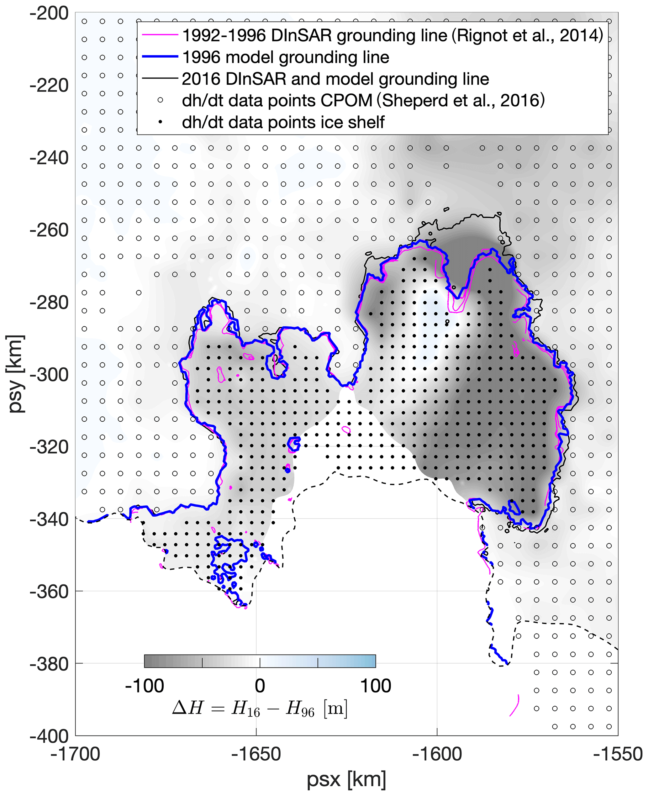
Figure A1 Ice thickness changes (ΔH) between 1996 and 2016, based on a comprehensive analysis of satellite altimeter data. The altimeter data coverage is represented by dots (ice shelf) and circles (grounded ice; Shepherd et al., 2016). The final 1996 ice thickness distribution was obtained by subtracting ΔH from the 2016 BedMachine ice thickness (Morlighem et al., 2020), as described in Sect.2.1. The associated 1996 grounding line location (blue line) compares well to independent DInSAR measurements (magenta line; Rignot et al., 2014).
The open source ice flow model Úa (Gudmundsson, 2020) uses the finite-element method to solve the shallow ice stream equations, commonly referred to as SSA or SSTREAM (Hutter, 1983; MacAyeal, 1989), on an irregular triangular mesh. The diagnostic velocity solver is based on an iterative Newton–Raphson method. A fixed mesh with 109 300 linear elements was used with a median nodal spacing of 1.2 km and local mesh refinement down to 500 m in areas with above-average horizontal shear, with strong gradients in ice thickness, and within a 10 km buffer around the grounding line. The mesh was generated using the open-source generator mesh2d (Engwirda, 2014).
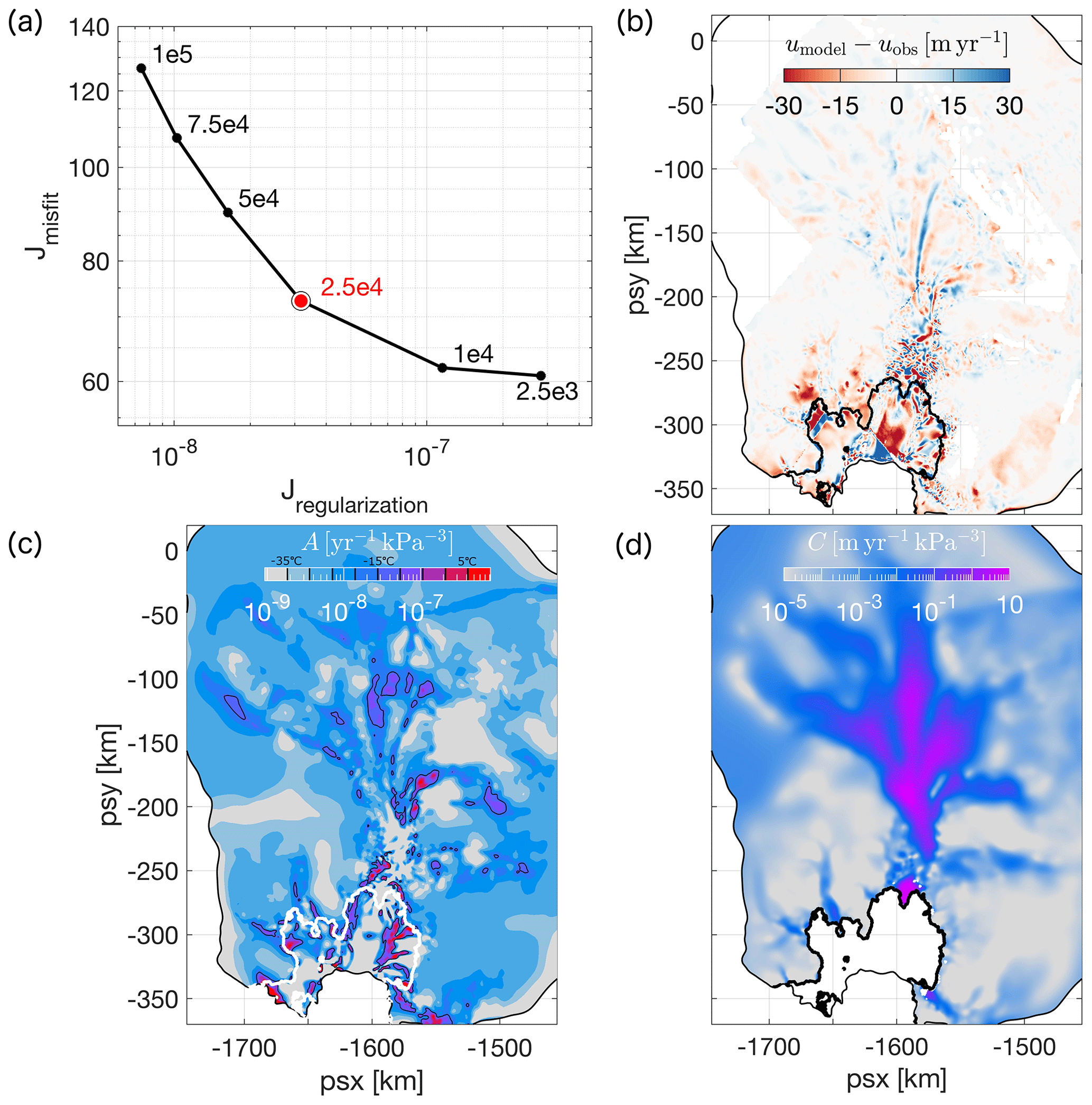
Figure B1 (a) L curve used to determine the optimal value of the Tikhonov regularization multiplier γs, highlighted in red. (b) Misfit between modelled and observed surface speed in 1996 for γs=25 000 m. (c) Rate factor (A in Eq. 2) in 1996, obtained as a minimum of the cost function J in Eq. (B1) with γs=25 000 m. The equivalent depth-averaged ice temperature ranges from −35 ∘C (grey) to 5 ∘C (red). Colours are discretized at 5 ∘C intervals, and the black lines indicate the 0 ∘C contour. The white line corresponds to the 1996 grounding line position. (d) Optimal value of the basal slipperiness (C in Eq. 3) in 1996, estimated using the adjoint minimization approach.
The optimization capabilities of Úa follow commonly applied techniques in ice flow modelling to optimize uncertain model parameters, pi, based on prior information, , and a range of observations with associated measurement errors (MacAyeal, 1992). Úa uses an adjoint method to obtain a combined optimal estimate of the spatially varying rate factor A and basal slipperiness C across the full model domain, for given observations of surface velocity uobs and measurement errors εu. Optimal values for were obtained as a solution to the minimization problem dpJ with the cost function J defined as the sum of the misfit term I and Tikhonov regularization R: , with
and being the total area of the model domain. An iterative interior point optimization algorithm was used to calculate dpJ and stopped after 104 iterations, when fractional changes to the cost function were less than 10−5.
The gradient and amplitude contributions in the regularization term (Eq. B2) are multiplied by spatially constant Tikhonov regularization multipliers, γi,s and γi,a. Optimal values for γi,s and γi,a were determined using an L-curve approach. For γi,s results are shown in Fig. B1. The values m were used for all experiments in the main part of the text, as they produced the smallest misfit between observed and modelled surface velocities whilst limiting the risk of overfitting. The sensitivity of the main results with respect to the choice of γs is discussed in Appendix D. A similar L-curve approach was followed to determine optimal values for γi,a, with used throughout this study.
The pre-multipliers γi,s and γi,a are constant across the model domain. Some studies set for grounded areas and only optimize the rate factor on the ice shelves. This approach assumes perfect prior knowledge about the spatial distribution and magnitude of the rate factor upstream of the grounding line, often tied to (uncertain) estimates of ice temperature. Here we prefer to optimize A across the full domain to allow for spatial variations in ice temperature, damage, fabric, and other ice properties for both floating and grounded ice. The amplitude and gradient of A, relative to a spatially constant prior value, are controlled by γA,a and γA,s respectively, with optimal values given above.
All results presented here are based on optimization experiments with spatially constant a priori values for the rate factor and slipperiness: kPa−3 yr−1, which corresponds to a spatially uniform ice temperature of −15 ∘C (Cuffey and Paterson, 2010), and , with ub=750 m yr−1 and τ=80 kPa and m being the sliding-law exponent. Different a priori values for the rate factor, equivalent to ice temperatures between −20 and −5 ∘C, were tested but did not cause significant differences in the results. We did not consider optimization experiments with spatially variable based on independent estimates of ice temperature and/or damage, since such estimates contain significant uncertainties at the regional scales considered in this study.
Figures B1b–d summarize the results for an optimization with m, , kPa−3 yr−1, and m yr−1 kPa−3. Modelled surface velocities are typically within 30 m per year or less of the observed values, with a mean misfit of and standard deviation of 15.3 m yr−1. The highest values of the rate factor are generally found within the shear margins, with positive equivalent ice temperatures suggesting the presence of a complex rheology or damage. The highest values of the slipperiness are consistently found in the fast-flowing central part of the glacier and along its upstream tributaries, with noticeably reduced values of C in an area between 5 and 40 km upstream of the 1996 grounding line. These results are broadly in agreement with previously published maps; see, for example, Arthern et al. (2015).
The transfer amplitude , defined in Eq. (4), describes the linear response of the along-slope surface velocity to small harmonic perturbations in the surface elevation or, equivalently, ice thickness. Analytical solutions for the transfer function 𝒯US (amplitude and phase) in the framework of the shallow ice stream approximation with a linear ice rheology (n=1 in Eq. 2) and a non-linear viscous sliding law (arbitrary m in Eq. 3) were previously obtained by Gudmundsson (2008). Note that the original expression (Eq. 29 in Gudmundsson, 2008) contained a printing error, so we repeat the correct form here:
where H is the local ice thickness; α is the local bed slope; ρ is the ice viscosity; τd=ρgHsinα is the driving stress; η is the effective viscosity; and , ψ=ikHcotα, and are abbreviations, with k and l the along-slope and transverse wavelength respectively of the harmonic surface perturbation. Since we focus on the instantaneous response of the velocity to perturbations at the surface, the exponential decay of 𝒯US with time has been omitted. An equivalent expression for the response of the transverse velocity component can be derived; we refer to Gudmundsson (2008) for more details.

Figure C1 (a) Goodness of fit between and model simulations . Red areas correspond to R2≥0.9 and fitting parameter f1≥100. An example of the fit at location 1 and resulting moptimal (Eq. 7) is shown in panel (b). Black areas in panel (a) correspond to R2≥0.9 and fitting parameter f1<100. The horizontal asymptote with limit <100 indicates that a positive, finite solution moptimal does not exist, and Weertman sliding cannot reproduce 100 % of the observed changes in surface velocity. An example of the fit and asymptote at location 2 is shown in panel (c). Grey areas in panel (a) correspond to R2<0.9, indicating a poor fit between and . An example at location 3 is shown in panel (d).
Following Gudmundsson (2008), physical quantities can be rescaled to obtain the non-dimensional form of the transfer function. After substitution of the scalings H→1, , and τd→1 into Eq. (C1) and some reordering, one obtains
The resulting transfer amplitude takes the form as in Eq. (4), where functions f1 and f2 depend on C, α, k, and l.
The analytical expression in Eq. (C2) describes the first-order response to small perturbations in ice thickness, δH≪1, for well-defined length scales characterized by k and l. However, in a realistic setting such as PIG, the system responds to a complicated perturbation composed of a range of wavelengths and amplitudes, and Eq. (C2) does not automatically hold. Based on experiments , presented in Sect. 3.3, we found that the simulated surface response of PIG to observed geometrical perturbations retains it dependency on m of the form , but more complicated expressions for f1 and f2 are required that do not exist in analytical form. A best estimate for the spatially varying fields f1 and f2 was obtained by minimizing the misfit between , and . The resulting misfit, quantified by R2 values, is summarized in Fig. C1a. Red and black areas indicate a good fit with R2≥0.9, though an important distinction was made between solutions with f1≥100 (red) and f1<100 (black). The difference between the two cases is explained further in Sect. 3.3. Examples of the fit at locations 1 and 2 are shown in Fig. C1b and c respectively. Grey shading in Fig. C1a corresponds to a poor fit (R2<0.9), and the dependency of on m cannot be adequately described by the function . Possible reasons for this discrepancy are discussed in Sect. 3.3.
The inverse problem of inferring information about the rate factor A and basal slipperiness C from uncertain observations of surface velocity is generally ill-posed. To remedy the ill-posedness of the problem, additional information in the form of a regularization term (Eq. B2) is commonly added to the cost function. The solution of the minimization problem generally depends on the choice of regularization. In the specific case of a Tikhonov regularization, which is used throughout this study, the solution for A and C will depend on the unknown multipliers γi,a and γi,s, and on the choice of prior information in Eq. (B2). One method of choosing an “optimal” value for the multipliers is the L-curve approach presented in Appendix B. However, this is an ad hoc method, and it remains to be shown that results are robust for a range of γ values. Below we discuss the robustness of our results for a range γs values. A similar analysis was carried out for a range of γa values and priors, but those results did not affect our conclusions and are not shown here.
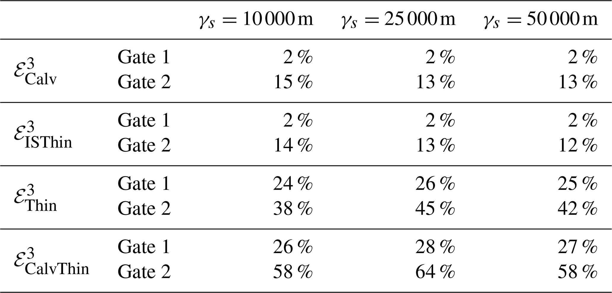
In the case of the perturbation experiments, which were designed to simulate the velocity response to a series of prescribed changes in the PIG geometry, we are primarily interested in the γs dependency of the relative fluxes in Fig. 3e. In addition to the experiments with default value γs=25 000 m, identical perturbation experiments were carried out for γs=10 000 m and γs=50 000 m. The corresponding changes in flux, presented in Table D1, do not show any significant variability with γs, and results presented in Sect. 3.1 can be considered robust, at least across the range of tested γs values.
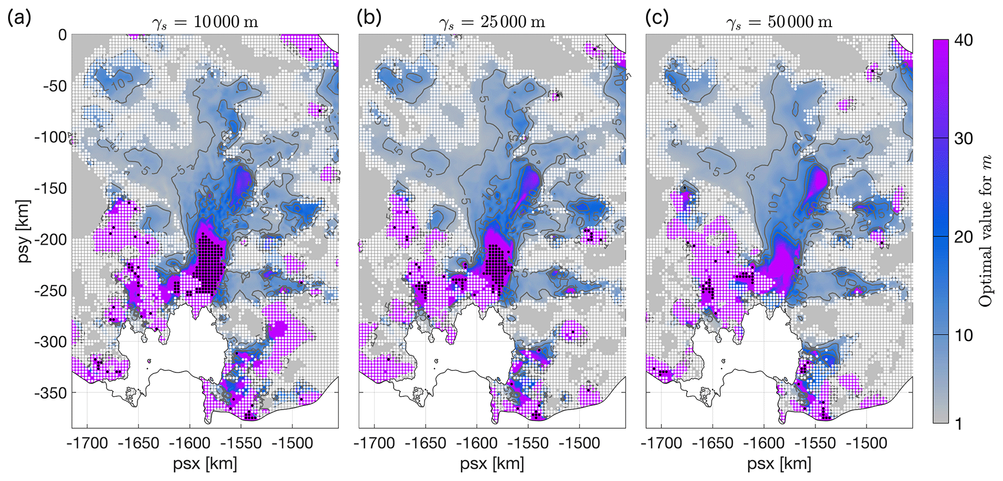
Figure D1 Optimal distribution of m, as in Fig. 6a, for different values of the regularization multiplier: (a) γs=10 000 m, (b) γs=25 000 m, and (c) γs=50 000 m. White dots indicate areas where results for the non-linear regression method were poor, with a R2 value smaller than 0.9. Black dots indicate areas where the value of f1 in the fit is less than 100, indicating that agreement between simulated and observed changes in surface velocity cannot be achieve for finite values of m. The value γs=25 000 m was used throughout the main part of this study.
Experiments and were also repeated for γs=10 000 m and γs=50 000 m. Maps of A and C (not shown) were compared to the default results for γs=25 000 m shown in Fig. 4, and no significant qualitative differences were found.
Perturbation experiments for a range of sliding-law exponents were repeated for γs=10 000 m and γs=50 000 m. Following the approach outlined in Sect. 3.3, an optimal spatial distribution of the sliding exponent was computed for each γs. Results are presented in Fig. D1 and show a decreasing trend in moptimal for increasing values of the regularization multiplier γs. In particular, the area where no positive, finite solution exists for moptimal (shaded in black) is reduced in size and eventually disappears for increasing amounts of regularization. However, the spatial distribution of moptimal is found to be in broad agreement across the considered range of γs.
The open-source ice flow model Úa is available at https://doi.org/10.5281/zenodo.3706623 (Gudmundsson, 2020). Unprocessed model output for all experiments presented in this paper are available at https://doi.org/10.17605/OSF.IO/TEKRF (De Rydt and Reese, 2020). Ice shelf thinning rates are available upon request from Fernando S. Paolo.
JDR and RR designed and initiated the project and prepared the manuscript. FSP processed the ice shelf thickness data. JDR performed the model simulations, carried out the analysis, and produced the figures. FSP and GHG reviewed and edited the paper.
Jan De Rydt serves as topical editor for The Cryosphere.
We would like to express our sincere appreciation for the thorough reviews by Stephen Cornford; two anonymous reviewers; and the editor, Andreas Vieli. Their insightful comments have greatly contributed to a better presentation of our work. Jan De Rydt, G. Hilmar Gudmundsson, and Ronja Reese are supported by the TiPACCs project, which receives funding from the European Union's Horizon 2020 research and innovation programme under grant agreement no. 820575. Ronja Reese is further supported by the Deutsche Forschungsgemeinschaft (DFG) by grant WI4556/3-1, and G. Hilmar Gudmundsson by the NSFPLR-NERC grant Processes, drivers, predictions: Modelling the response of Thwaites Glacier over the next century using ice/ocean coupled models (NE/S006745/1).
This research has been supported by the European Union's Horizon 2020 research and innovation programme (grant no. 820575), the Deutsche Forschungsgemeinschaft (DFG) (grant no. WI4556/3-1), and the NSFPLR-NERC (grant no. NE/S006745/1).
This paper was edited by Andreas Vieli and reviewed by Stephen Cornford and two anonymous referees.
Alley, K. E., Scambos, T. A., Alley, R. B., and Holschuh, N.: Troughs developed in ice-stream shear margins precondition ice shelves for ocean-driven breakup, Sci. Adv., 5, 1–8, https://doi.org/10.1126/sciadv.aax2215, 2019. a, b, c
Arndt, J. E., Larter, R. D., Friedl, P., Gohl, K., Höppner, K., and the Science Team of Expedition PS104: Bathymetric controls on calving processes at Pine Island Glacier, The Cryosphere, 12, 2039–2050, https://doi.org/10.5194/tc-12-2039-2018, 2018. a, b, c
Arthern, R. J. and Williams, C. R.: The sensitivity of West Antarctica to the submarine melting feedback, Geophys. Res. Lett., 44, 2352–2359, https://doi.org/10.1002/2017GL072514, 2017. a
Arthern, R. J., Hindmarsh, R. C., and Williams, C. R.: Flow speed within the Antarctic ice sheet and its controls inferred from satellite observations, J. Geophys. Res.-Earth, 120, 1171–1188, https://doi.org/10.1002/2014JF003239, 2015. a
Bamber, J. L. and Bindschadler, R. A.: An improved elevation dataset for climate and ice-sheet modelling: validation with satellite imagery, Ann. Glaciol., 25, 439–444, https://doi.org/10.3189/S0260305500014427, 1997. a
Bamber, J. L. and Dawson, G. J.: Complex evolving patterns of mass loss from Antarctica’s largest glacier, Nat. Geosci., 13, 127–131, 2020. a, b, c
Brondex, J., Gillet-Chaulet, F., and Gagliardini, O.: Sensitivity of centennial mass loss projections of the Amundsen basin to the friction law, The Cryosphere, 13, 177–195, https://doi.org/10.5194/tc-13-177-2019, 2019. a, b, c
Budd, W. F., Jenssen, D., and Smith, I. N.: A Three-Dimensional Time-Dependent Model of the West Antarctic Ice Sheet, Ann. Glaciol., 5, 29–36, https://doi.org/10.3189/1984AoG5-1-29-36, 1984. a
Christianson, K., Bushuk, M., Dutrieux, P., Parizek, B. R., Joughin, I. R., Alley, R. B., Shean, D. E., Abrahamsen, E. P., Anandakrishnan, S., Heywood, K. J., Kim, T.-W., Lee, S. H., Nicholls, K., Stanton, T., Truffer, M., Webber, B. G. M., Jenkins, A., Jacobs, S., Bindschadler, R., and Holland, D. M.: Sensitivity of Pine Island Glacier to observed ocean forcing, Geophys. Res. Lett., 43, 10817–10825, https://doi.org/10.1002/2016GL070500, 2016. a
Chuter, S. J. and Bamber, J. L.: Antarctic ice shelf thickness from CryoSat-2 radar altimetry, Geophys. Res. Lett., 42, 10721–10729, https://doi.org/10.1002/2015GL066515, 2015. a
Cuffey, K. and Paterson, W.: The physics of glaciers, 4th Edition, Elsevier, ISBN 9780123694614, https://doi.org/10.1016/0016-7185(71)90086-8, 2010. a
De Rydt, J. and Reese, R.: Model output for `Drivers of Pine Island Glacier speed-up between 1996 and 2016', OSF, https://doi.org/10.17605/OSF.IO/TEKRF, 2020. a
Dutrieux, P., De Rydt, J., Jenkins, A., Holland, P. R., Ha, H. K., Lee, S. H., Steig, E. J., Ding, Q., Abrahamsen, E. P., and Schröder, M.: Strong sensitivity of Pine Island ice-shelf melting to climatic variability, Science, 343, 174–178, 2014. a
Engwirda, D.: Locally-optimal Delaunay-refinement and optimisation-based mesh generation, PhD thesis, The University of Sydney, http://hdl.handle.net/2123/13148, 2014. a
Favier, L., Durand, G., Cornford, S., Gudmundsson, G., Gagliardini, O., Gillet-Chaulet, F., Zwinger, T., Payne, A., and Brocq, A.: Retreat of Pine Island Glacier controlled by marine ice-sheet instability, Nature Clim. Change, 4, 117–121, https://doi.org/10.1038/nclimate2094, 2014. a, b
Gardner, A. S., Moholdt, G., Scambos, T., Fahnstock, M., Ligtenberg, S., van den Broeke, M., and Nilsson, J.: Increased West Antarctic and unchanged East Antarctic ice discharge over the last 7 years, The Cryosphere, 12, 521–547, https://doi.org/10.5194/tc-12-521-2018, 2018. a, b
Gillet-Chaulet, F., Durand, G., Gagliardini, O., Mosbeux, C., Mouginot, J., Rémy, F., and Ritz, C.: Assimilation of surface velocities acquired between 1996 and 2010 to constrain the form of the basal friction law under Pine Island Glacier, Geophys. Res. Lett., 43, 10311–10321, 2016. a, b, c, d, e
Gudmundsson, G. H.: Analytical solutions for the surface response to small amplitude perturbations in boundary data in the shallow-ice-stream approximation, The Cryosphere, 2, 77–93, https://doi.org/10.5194/tc-2-77-2008, 2008. a, b, c, d, e, f
Gudmundsson, G. H.: GHilmarG/UaSource: Ua2019b (Version v2019b), Zenodo, https://doi.org/10.5281/zenodo.3706623, 2020. a, b, c, d
Gudmundsson, G. H., Krug, J., Durand, G., Favier, L., and Gagliardini, O.: The stability of grounding lines on retrograde slopes, The Cryosphere, 6, 1497–1505, https://doi.org/10.5194/tc-6-1497-2012, 2012. a
Gudmundsson, G. H., Paolo, F. S., Adusumilli, S., and Fricker, H. A.: Instantaneous Antarctic ice sheet mass loss driven by thinning ice shelves, Geophys. Res. Lett., 46, 13903–13909, https://doi.org/10.1029/2019GL085027, 2019. a, b, c
Howat, I. M., Porter, C., Smith, B. E., Noh, M.-J., and Morin, P.: The Reference Elevation Model of Antarctica, The Cryosphere, 13, 665–674, https://doi.org/10.5194/tc-13-665-2019, 2019 a
Hutter, K.: Theoretical Glaciology: Material Science of Ice and the Mechanics of Glaciers and Ice Sheets, Mathematical Approaches to Geophysics, Springer, Dordrecht, 1983. a
Jenkins, A., Dutrieux, P., Jacobs, S., Mcphail, S., Perrett, J., Webb, A., and White, D.: Observations beneath Pine Island Glacier in West Antarctica and implications for its retreat, Nat. Geosci., 3, 468–472, https://doi.org/10.1038/ngeo890, 2010. a
Jenkins, A., Dutrieux, P., Jacobs, S., Steig, E., Gudmundsson, G., Smith, J., and Heywood, K.: Decadal Ocean Forcing and Antarctic Ice Sheet Response: Lessons from the Amundsen Sea, Oceanography, 29, 106–117, https://doi.org/10.5670/oceanog.2016.103, 2016. a
Joughin, I., Tulaczyk, S., Bamber, J. L., Blankenship, D., Holt, J. W., Scambos, T., and Vaughan, D. G.: Basal conditions for Pine Island and Thwaites Glaciers, West Antarctica, determined using satellite and airborne data, J. Glaciol., 55, 245–257, https://doi.org/10.3189/002214309788608705, 2009. a
Joughin, I., Smith, B. E., and Holland, D. M.: Sensitivity of 21st century sea level to ocean-induced thinning of Pine Island Glacier, Antarctica, Geophys. Res. Lett., 37, L20502, https://doi.org/10.1029/2010GL044819, 2010. a, b, c, d
Joughin, I., Smith, B. E., and Schoof, C. G.: Regularized Coulomb friction laws for ice sheet sliding: application to Pine Island Glacier, Antarctica, Geophys. Res. Lett., 46, 4764–4771, 2019. a, b, c, d, e, f, g, h
Khazendar, A., Rignot, E., and Larour, E.: Larsen B Ice Shelf rheology preceding its disintegration inferred by a control method, Geophys. Res. Lett., 34, 1–6, https://doi.org/10.1029/2007GL030980, 2007. a
Lhermitte, S., Sun, S., Shuman, C., Wouters, B., Pattyn, F., Wuite, J., Berthier, E., and Nagler, T.: Damage accelerates ice shelf instability and mass loss in Amundsen Sea Embayment, P. Natl. Acad. Sci. USA, 117, 24735–24741, https://doi.org/10.1073/pnas.1912890117, 2020. a
MacAyeal, D. R.: Large-scale ice flow over a viscous basal sediment: Theory and application to ice stream B, Antarctica, J. Geophys. Res.-Sol. Ea., 94, 4071–4087, https://doi.org/10.1029/JB094iB04p04071, 1989. a
MacAyeal, D. R.: The basal stress distribution of ice stream E, Antarctica, inferred by control methods, J. Geophys. Res., 97, 595–603, https://doi.org/10.1029/91JB02454, 1992. a, b
McMillan, M., Shepherd, A., Sundal, A., Briggs, K., Muir, A., Ridout, A., Hogg, A., and Wingham, D.: Increased ice losses from Antarctica detected by CryoSat-2, Geophys. Res. Lett., 41, 3899–3905, https://doi.org/10.1002/2014GL060111, 2014. a
Minchew, B., Simons, M., Björnsson, H., Pálsson, F., Morlighem, M., Seroussi, H., Larour, E., and Hensley, S.: Plastic bed beneath Hofsjökull Ice Cap, central Iceland, and the sensitivity of ice flow to surface meltwater flux, J. Glaciol., 62, 147–158, https://doi.org/10.1017/jog.2016.26, 2016. a
Morlighem, M., Rignot, E., Binder, T., Blankenship, D., Drews, R., Eagles, G., Eisen, O., Ferraccioli, F., Forsberg, R., Fretwell, P., Goel, V., Greenbaum, J. S., Gudmundsson, H., Guo, J., Helm, V., Hofstede, C., Howat, I., Humbert, A., Jokat, W., Karlsson, N. B., Lee, W. S., Matsuoka, K., Millan, R., Mouginot, J., Paden, J., Pattyn, F., Roberts, J., Rosier, S., Ruppel, A., Seroussi, H., Smith, E. C., Steinhage, D., Sun, B., den Broeke, M. R., Ommen, T. D., van Wessem, M., and Young, D. A.: Deep glacial troughs and stabilizing ridges unveiled beneath the margins of the Antarctic ice sheet, Nat. Geosci., 13, 132–137, https://doi.org/10.1038/s41561-019-0510-8, 2020. a, b, c
Mouginot, J., Rignot, E., and Scheuchl, B.: Sustained increase in ice discharge from the Amundsen Sea Embayment, West Antarctica, from 1973 to 2013, Geophys. Res. Lett., 41, 1576–1584, 2014. a
Mouginot, J., Rignot, E., and Scheuchl, B.: MEaSUREs Phase-Based Antarctica Ice Velocity Map, Version 1, https://doi.org/10.5067/PZ3NJ5RXRH10 (last access: 1 October 2019), 2019a. a, b, c
Mouginot, J., Rignot, E., and Scheuchl, B.: Continent-Wide, Interferometric SAR Phase, Mapping of Antarctic Ice Velocity, Geophys. Res. Lett., 46, 9710–9718, https://doi.org/10.1029/2019GL083826, 2019b. a, b
Nilsson, J., Gardner, A., Sandberg Sørensen, L., and Forsberg, R.: Improved retrieval of land ice topography from CryoSat-2 data and its impact for volume-change estimation of the Greenland Ice Sheet, The Cryosphere, 10, 2953–2969, https://doi.org/10.5194/tc-10-2953-2016, 2016. a, b
Padman, L., Fricker, H. A., Coleman, R., Howard, S., and Erofeeva, L.: A new tide model for the Antarctic ice shelves and seas, Ann. Glaciol., 34, 247–254, https://doi.org/10.3189/172756402781817752, 2002. a
Padman, L., King, M., Goring, D., Corr, H., and Coleman, R.: Ice-shelf elevation changes due to atmospheric pressure variations, J. Glaciol., 49, 521–526, https://doi.org/10.3189/172756503781830386, 2004. a
Paolo, F., Padman, L., Fricker, H., Adusumilli, S., Howard, S., and Siegfried, M.: Response of Pacific-sector Antarctic ice shelves to the El Niño/Southern Oscillation, Nat. Geosci., 11, 121–126, https://doi.org/10.1038/s41561-017-0033-0, 2018. a
Paolo, F. S., Fricker, H. A., and Padman, L.: Constructing improved decadal records of Antarctic ice shelf height change from multiple satellite radar altimeters, Remote Sens. Environ., 177, 192–205, https://doi.org/10.1016/j.rse.2016.01.026, 2016. a, b
Payne, A. J., Vieli, A., Shepherd, A. P., Wingham, D. J., and Rignot, E.: Recent dramatic thinning of largest West Antarctic ice stream triggered by oceans, Geophys. Res. Lett., 31, 1–4, https://doi.org/10.1029/2004GL021284, 2004. a, b
Pritchard, H., Arthern, R., Vaughan, D., and Edwards, L.: Extensive dynamic thinning on the margins of the Greenland and Antarctic Ice Sheets, Nature, 461, 971–975, https://doi.org/10.1038/nature08471, 2009. a
Pritchard, H., Ligtenberg, S., Fricker, H., Vaughan, D., Van den Broeke, M., and Padman, L.: Antarctic ice-sheet loss driven by basal melting of ice shelves, Nature, 484, 502–505, https://doi.org/10.1038/nature10968, 2012. a
Reese, R., Gudmundsson, G. H., Levermann, A., and Winkelmann, R.: The far reach of ice-shelf thinning in Antarctica, Nat. Clim. Change, 8, 53–57, https://doi.org/10.1038/s41558-017-0020-x, 2018. a, b, c
Rignot, E.: Changes in West Antarctic ice stream dynamics observed with ALOS PALSAR data, Geophys. Res. Lett., 35, L12505, https://doi.org/10.1029/2008GL033365, 2008. a, b
Rignot, E., Vaughan, D. G., Schmeltz, M., Dupont, T., and Macayeal, D.: Acceleration of Pine Island and Thwaites Glaciers, West Antarctica, Ann. Glaciol., 34, 189–194, https://doi.org/10.3189/172756402781817950, 2002. a, b
Rignot, E., Mouginot, J., and Scheuchl, B.: Ice Flow of the Antarctic Ice Sheet, Science, 333, 1427–1430, https://doi.org/10.1126/science.1208336, 2011. a, b, c
Rignot, E., Mouginot, J., Morlighem, M., Seroussi, H., and Scheuchl, B.: Widespread, rapid grounding line retreat of Pine Island, Thwaites, Smith, and Kohler glaciers, West Antarctica, from 1992 to 2011, Geophys. Res. Lett., 41, 3502–3509, 2014. a, b, c, d, e, f, g, h
Rosier, S. H. R., Reese, R., Donges, J. F., De Rydt, J., Gudmundsson, G. H., and Winkelmann, R.: The tipping points and early-warning indicators for Pine Island Glacier, West Antarctica, The Cryosphere Discuss. [preprint], https://doi.org/10.5194/tc-2020-186, in review, 2020. a
Schmeltz, M., Rignot, E., Dupont, T. K., and Macayeal, D. R.: Sensitivity of Pine Island Glacier, West Antarctica, to changes in ice-shelf and basal conditions: A model study, J. Glaciol., 48, 552–558, https://doi.org/10.3189/172756502781831061, 2002. a, b, c
Schoof, C.: Variational methods for glacier flow over plastic till, J. Fluid Mech., 555, 299–320, https://doi.org/10.1017/S0022112006009104, 2006. a
Seroussi, H., Morlighem, M., Rignot, E., Mouginot, J., Larour, E., Schodlok, M., and Khazendar, A.: Sensitivity of the dynamics of Pine Island Glacier, West Antarctica, to climate forcing for the next 50 years, The Cryosphere, 8, 1699–1710, https://doi.org/10.5194/tc-8-1699-2014, 2014. a, b
Shepherd, A., Wingham, D., Mansley, J., and Corr, H.: Inland Thinning of Pine Island Glacier, West Antarctica, Science, 291, 862–864, https://doi.org/10.1126/science.291.5505.862, 2001. a
Shepherd, A., Wingham, D., and Rignot, E.: Warm ocean is eroding West Antarctic ice sheet, Geophys. Res. Lett., 31, 402, https://doi.org/10.1029/2004GL021106, 2004. a
Shepherd, A., Hogg, A., Muir, A., and McMillan, M.: Surface Elevation Changes of the Antarctic Ice Sheet from Satellite Radar Altimetry, Antarctic-CCI-SEC-v1.0, available at: http://www.cpom.ucl.ac.uk/csopr/icesheets2/, 2016. a, b, c, d
Smith, J. A., Andersen, T. J., Shortt, M., Gaffney, A., Truffer, M., Stanton, T., Bindschadler, R., Dutrieux, P., Jenkins, A., Hillenbrand, C.-D., Ehrmann, W., Corr, H. F. J., Farley, N., Crowhurst, S., and Vaughan, D. G.: Sub-ice-shelf sediments record history of twentieth-century retreat of Pine Island Glacier, Nature, 541, 77–80, 2017. a
Steig, E., Ding, Q., Battisti, D., and Jenkins, A.: Tropical forcing of Circumpolar Deep Water Inflow and outlet glacier thinning in the Amundsen Sea Embayment, West Antarctica, Ann. Glaciol., 53, 19–28, https://doi.org/10.3189/2012AoG60A110, 2012. a
Sun, S., Cornford, S. L., Moore, J. C., Gladstone, R., and Zhao, L.: Ice shelf fracture parameterization in an ice sheet model, The Cryosphere, 11, 2543–2554, https://doi.org/10.5194/tc-11-2543-2017, 2017. a
Tsai, V. C., Stewart, A. L., and Thompson, A. F.: Marine ice-sheet profiles and stability under Coulomb basal conditions, J. Glaciol., 61, 205–215, https://doi.org/10.3189/2015JoG14J221, 2015. a
Tulaczyk, S., Kamb, W. B., and Engelhardt, H. F.: Basal mechanics of Ice Stream B, west Antarctica: 1. Till mechanics, J. Geophys. Res.-Sol. Ea., 105, 463–481, https://doi.org/10.1029/1999JB900329, 2000. a
Vieli, A., Payne, A. J., Shepherd, A., and Du, Z.: Causes of pre-collapse changes of the Larsen B ice shelf: Numerical modelling and assimilation of satellite observations, Earth Planet. Sc. Lett., 259, 297–306, https://doi.org/10.1016/j.epsl.2007.04.050, 2007. a
Weertman, J.: On the sliding of glaciers, J. Glaciol., 3, 33–38, 1957. a, b
Zoet, L. K. and Iverson, N. R.: A slip law for glaciers on deformable beds, Science, 368, 76–78, https://doi.org/10.1126/SCIENCE.AAZ1183, 2020. a
- Abstract
- Introduction and motivation
- Data and methods
- Results and discussion
- Conclusions
- Appendix A: Observations of Pine Island Ice Shelf thickness changes between 1996 and 2016
- Appendix B: Model configuration and optimization
- Appendix C: Non-linear dependency of the flow response on the sliding exponent
- Appendix D: Dependency of the results on the regularization
- Code and data availability
- Author contributions
- Competing interests
- Acknowledgements
- Financial support
- Review statement
- References