the Creative Commons Attribution 4.0 License.
the Creative Commons Attribution 4.0 License.
 | 05 Mar 2020
Brief communication: On calculating the sea-level contribution in marine ice-sheet models
Violaine Coulon
Frank Pattyn
Bas de Boer
Roderik van de Wal
Estimating the contribution of marine ice sheets to sea-level rise is complicated by ice grounded below sea level that is replaced by ocean water when melted. The common approach is to only consider the ice volume above floatation, defined as the volume of ice to be removed from an ice column to become afloat. With isostatic adjustment of the bedrock and external sea-level forcing that is not a result of mass changes of the ice sheet under consideration, this approach breaks down, because ice volume above floatation can be modified without actual changes in the sea-level contribution. We discuss a consistent and generalised approach for estimating the sea-level contribution from marine ice sheets.
Please read the corrigendum first before continuing.
-
Notice on corrigendum
The requested paper has a corresponding corrigendum published. Please read the corrigendum first before downloading the article.
-
Article
(510 KB)
- Corrigendum
-
Supplement
(241 KB)
-
The requested paper has a corresponding corrigendum published. Please read the corrigendum first before downloading the article.
- Article
(510 KB) - Full-text XML
- Corrigendum
-
Supplement
(241 KB) - BibTeX
- EndNote


Model simulations of past and future ice-sheet evolution are an important tool to understand and estimate the contribution of ice sheets to sea level at different timescales (e.g. de Boer et al., 2015; Nowicki et al., 2016). The mass balance of ice sheets is controlled by mass gain and loss at the upper, lower and lateral boundaries by melting or sublimation, by accumulation and freeze-on, and by discharge of ice into the surrounding oceans. The sea-level contribution from an ice sheet can in principle be estimated through these different mass balance terms but is in practice typically based on changes in one prognostic variable, ice thickness, and considering corrections for the ice grounded below sea level (e.g. Bamber et al., 2013). However, complications arise, especially for longer timescales, when isostatic adjustment of the bedrock is considered. The discussions in this communication apply for ice-sheet models that include some form of a glacio-isostatic adjustment (GIA), but that are not coupled to the sea-level equation. While other examples exist (e.g. Gomez et al., 2013; de Boer et al., 2014), the models considered here typically account strictly for uplift or sinking of the bedrock beneath or proximal to an ice sheet but do not include other (global) effects, such as sea-level changes due to changes in Earth's rotation and regional sea-level change due to changes in the Earth's gravitational field. However, the effect of mass changes from other ice sheets may be included in a simplified form using an external sea-level forcing. Such forcing is decoupled from mass changes of the ice sheet itself and prescribes sea-level changes in the model domain with the aim to capture its effect on ice floatation. The aim of this paper is to propose an approach to accurately estimate the contribution of the ice sheet in such a model to global-mean geocentric sea-level rise (see Gregory et al., 2019).
In our own ice-sheet modelling experience and from exchange with colleagues in different groups, it is not always clear how the sea-level contribution should exactly be calculated and what corrections need to be applied. This goes hand in hand with a lack of documentation and transparency in the published literature on how the sea-level contribution is estimated in different models. With this brief communication, we hope to stimulate awareness and discussion in the community to improve on this situation. We caution that it is very possible that the proposed solutions or equivalent approaches are already in use in several models, since the fundamental ideas have already been laid out (e.g. Bamber et al., 2013; de Boer et al., 2015) and are straightforward to implement. Our aim here is to provide concrete guidelines and a central reference of best practices for ice-sheet modellers.
We describe in the following how to calculate the sea-level contribution for a situation without bedrock changes (Sect. 1), the effect of bedrock changes and how to account for them (Sects. 2 and 3), a density correction (Sect. 4), and modifications required when the model is forced by external sea-level changes (Sect. 5). We conclude with a realistic modelling example (Sect. 6) and a discussion (Sect. 7).
If changes in the bedrock elevation due to isostatic adjustment are zero or very small, e.g. for centennial timescale simulations (e.g. Nowicki et al., 2016), the sea-level contribution of an ice sheet is typically computed from changes in total ice volume above floatation:
where H is ice thickness, b is bedrock elevation (negative if below sea level), and ρice=910 kg m−3 and ρocean=1028 kg m−3 are the densities of ice and ocean water, respectively. The sum is over the number n of grid cells (elements) of an (un-)structured grid with area An. The unitless map scale factor k is applied when the model grid is laid out on a projected horizontal coordinate system, which is often the case for polar ice-sheet models (Snyder, 1987; Reerink et al., 2016). Below, we will often simplify the discussion in order to examine the interplay between ice-sheet thickness, bedrock elevation, and sea level for a single column, which can be conceptualised as the values occurring in any single model grid cell or element (in map view). In that framework, we will refer to the limit ice thickness required for the ice to start floating as the floatation thickness, which is determined by the local bedrock elevation and sea level. Vaf of a column of ice grounded below sea level may be interpreted as the amount of ice volume that has to be removed to reach the floatation thickness and for the column to start to float. This considers that floating ice is in hydrostatic balance with the surrounding water and assumes that the ice does not contribute to sea-level changes when melted. In reality, however, densities of sea water and melted land ice (freshwater) differ slightly, which is often neglected. An associated density correction is discussed below (Sect. 4). For ice grounded on land above sea level, b>0 and .
To estimate the ice volume in global sea-level equivalent (SLEaf, m), the total Vaf has to be converted into the volume it will occupy when added to the ocean assuming a seawater density ρocean=1028 kg m−3 and divided by the ocean area Aocean of typically 3.625×10¹⁴ m2 (Gregory et al., 2019).
Aocean is assumed to be constant here, but on longer timescales this is not necessarily correct. Estimating changes in Aocean correctly would require a fully coupled model of global ice sheet–GIA–sea level (e.g. Gomez et al., 2013; de Boer et al., 2014). The actual sea-level contribution of the modelled ice sheet (SLC) is typically calculated relative to a reference value, often the present-day (modelled) configuration or the configuration at the start or end of an experiment.
Note that the minus sign in front of the parentheses in Eq. (3) is necessary since SLEaf is a function of Vaf, for which an increase over time is associated with a drop in sea level.
Depending on the amount of ice grounded below sea level, estimating the sea-level contribution instead from the entire grounded ice volume Vgr (Eq. 4) can lead to considerable biases and is only shown for comparison here.
In this section we discuss additional considerations that are required when the model includes a GIA component that simulates bedrock changes. When changes in bedrock elevation occur under the ice, Vaf cannot always be used without a correction as basis for sea-level calculations, because isostatic uplift or lowering can modify Vaf without actual sea-level contribution. Figure 1 illustrates this problem for a single ice column with an uplift of the bedrock elevation (left to right in each panel), where the bars indicate the bedrock and ice for different possible configurations. In case A, bedrock is already above sea level (i.e. Vaf includes all ice) and the vertical upward displacement has no apparent influence on the grounded configuration. In case B, ice is displaced upwards with the bedrock, the floatation thickness decreases and some of the ice is “transformed” into ice above floatation. In case C a transition from floating to grounded ice occurs, and in case D ocean water is displaced by the rising bedrock.
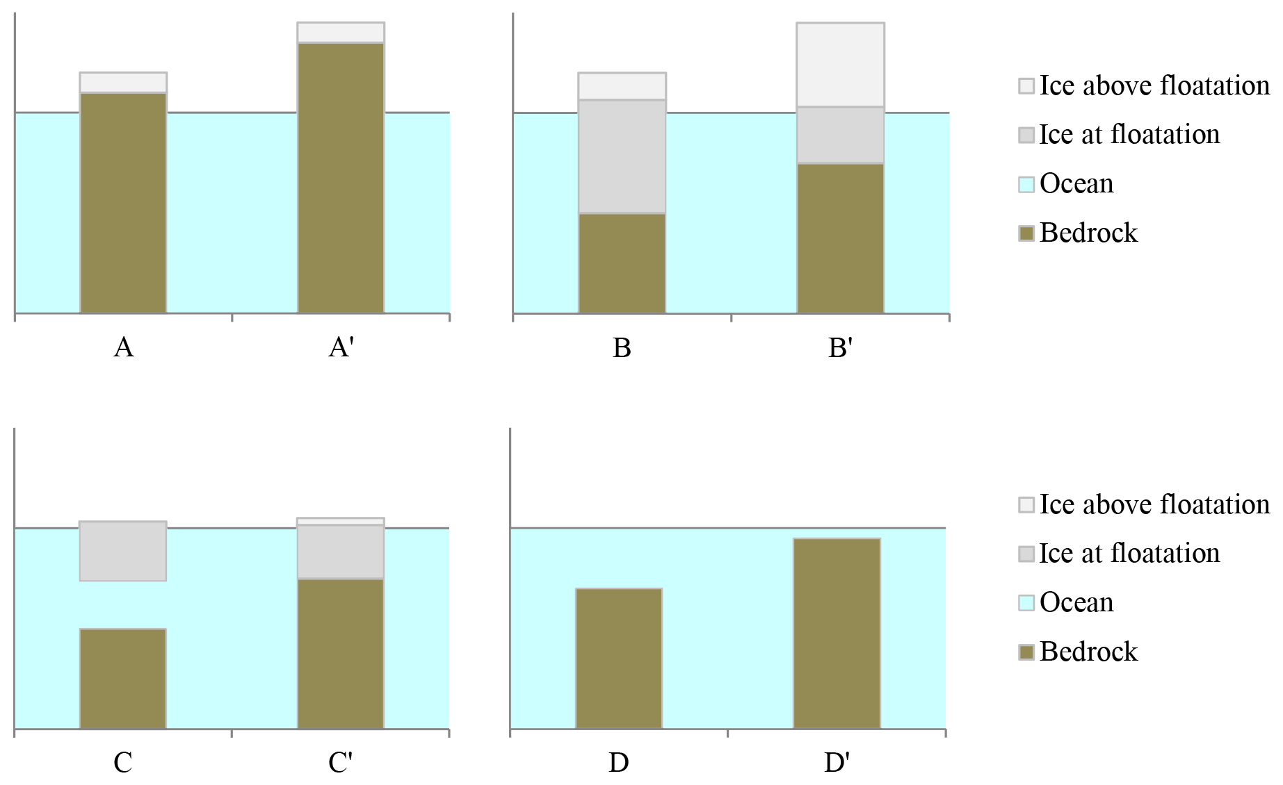
Figure 1Effect of bedrock changes. Different geometric configurations of ice, ocean and bedrock before and after (′) a rise in bedrock elevation.
The problem of how to interpret these changes in sea-level contribution in the presence of bedrock changes is further illustrated by an evolution of one grid box in time (Fig. 2a). If we compare between t1 and t4 and only look at the ice column, we could assume that there was no net sea-level contribution since the ice is just starting to float (t1) or floating (t4) in both cases. However, following the evolution through t2 and t3 gives rise to another interpretation. At t1 the ice is just starting to float with a low bedrock elevation. The bedrock then rises (t2) and subsequently ice is lost, for example by surface melting (t3). Finally, more ice is lost, for example by basal melting, and the ice is floating at t4. From t1 to t2, ice is merely displaced by the bedrock, but the actual sea-level contribution occurs between t2 and t3 and equals the ice above floatation in t2 and (by construction) also the bedrock displacement between t1 and t4.
The differences in sea-level contribution from t1 to t4 must be independent from the interpretation of what happened between t1 and t4. Hence, bedrock changes have to be taken into account below the ice and in proximity to the ice sheet. The way bedrock changes impact sea level is through changes in the volume of the ocean basins. That is, as bedrock is uplifted, ocean basin volume decreases, leading to a positive sea-level contribution and vice versa.
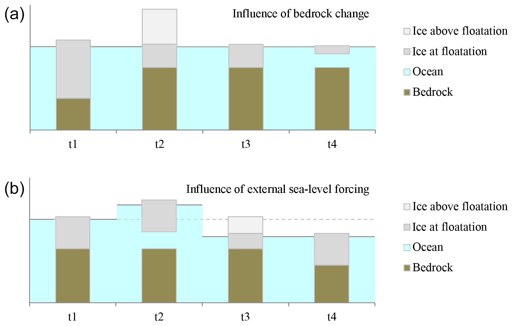
Figure 2Geometric evolution of a grid box in time (a) including bedrock changes and (b) including externally forced sea-level variations.
Based on the discussion in the previous section, here we propose an approach to correct the sea-level estimate for bedrock changes. Under floating ice and ice-free ocean, rising bedrock displaces ocean water and directly leads to a sea-level rise proportional to the bedrock elevation change. The additional sea-level contribution could be calculated from changes in the volume of the ocean water:
where the term in brackets is the difference between lower ice boundary and bedrock for grid cells containing floating ice and the ocean depth where no ice is present.
However, while bedrock changes under grounded ice have no impact on the estimated ocean volume, they do modify the amount of Vaf, which requires an additional correction. Consider an ice column near floatation but grounded below sea level at b0, with a height above floatation haf=0 (e.g. t1 in Fig. 2a). When the bedrock rises by a certain amount Δb (e.g. transition t1 to t2 in Fig. 2a), the ice is lifted and haf (in metres of ice equivalent) increases by
If the sea-level contribution was only computed from differences in total ice volume above floatation (SLEaf), this would be incorrectly recorded as a sea-level lowering. Furthermore, if the bedrock was lifted to or above sea level, the final change in haf would equal the ice thickness and
where b0 is the initial bedrock elevation (e.g. at t1 in Fig. 2a).
In order to consider corrections for bedrock changes under grounded ice, floating ice and ice-free ocean consistently, we chose to modify the ocean volume estimate to incorporate bedrock changes. Note that we assume in the following that all bedrock adjustment occurs within the ice-sheet model domain. We suggest replacing the ocean volume calculation above with an estimate of the potential ocean volume (Vpov), i.e. the volume between bedrock and sea level if all ice were instantaneously removed:
which requires no distinction anymore between grounded and floating ice. However, we have ignored the density difference between ocean water and freshwater, which we will treat separately below.
To convert a change in potential ocean volume to a sea-level contribution, Vpov has to be divided by the ocean area of typically 3.625×10¹⁴ m2:
In this section we discuss the correction necessary to deal with the small difference between freshwater (melted ice) and saline ocean water densities. Transitions of ice below and above floatation and the associated sea-level change can occur both due to ice mass changes and due to bedrock changes, processes associated with a different density (ρwater vs ρocean). While changes in Vaf due to bedrock adjustment and cavity changes are recorded in ocean water equivalent, we must assume that changes in ice-sheet mass ultimately contribute to the ocean with a density of freshwater (ρwater=1000 kg m−3). So far, we have calculated all changes in ocean water column equivalent, so now we will apply a density correction for all changes in ice thickness (above and below floatation).
The density ratio ρwater∕ρocean implies that the correction amounts to ∼3 % of the ice volume grounded at or below sea level.
Finally, to calculate changes in global-mean sea level due to ice-sheet changes, contributions from ice volume above floatation, potential ocean volume and density correction are added:
For long-term ice-sheet simulations, it is common to force ice-sheet models with prescribed variations in (global) sea level, e.g. representing changes in the Northern Hemisphere ice sheets when solely simulating the Antarctic ice sheet. For a glacial–interglacial transition the external sea-level forcing (ESLF) may have an amplitude of more than 100 m and can drive transitions between floating and grounded ice in the model. In the framework of such simulations, the calculation of sea-level contributions from the ice sheet must be re-considered, because changes in ESLF imply changes in Vaf of the modelled ice sheet.
We illustrate the implied changes again with a schematic view of one ice column changing over time (Fig. 2b). From t1 to t2, the sea level (horizontal solid line) is increased with respect to the starting value (horizontal dashed line) at constant bedrock elevation and ice thickness. Consequently, the geometry in the model column changes from just grounded to floating ice (with no sea-level contribution from the ice sheet itself). From t2 to t3 the sea level is lowered, such that some ice that was floating in t2 is transformed into ice above floatation. At t4, now with combined bedrock change and sea-level change of the same magnitude relative to t1, the ice is just grounded on the lowered bedrock. Calculating the sea-level contribution as described above in Eq. (12) would indicate a change of the contribution from t1 to t2 and t3. However, since these changes in sea level are externally forced, they should not directly contribute to the calculated ice-sheet sea-level contribution itself. For example, the additional volume under the floating ice at t2 occurs because the ice is lifted by the additional, externally forced seawater. Equally, the additional ice above floatation created in t3 is merely a consequence of the lower sea level. Hence, Vaf has to be corrected to calculate SLC in this case.
This problem can be resolved by calculating changes in Vaf and Vpov for the constructed case where sea level is fixed and ESLF has no direct impact on the results. Practically, Eqs. (1) and (8) can be modified to compensate for changes in bn that occur solely due to ESLF by corresponding changes in an arbitrary reference level z0, e.g. taken as present-day sea level, that is time-constant in the absolute reference frame but changes with ESLF (Eqs. 13, 14). In other words, the term (bn−z0) is constant with respect to changes in ESLF.
The density correction in Eq. (10) remains unchanged, leading with Eqs. (3) and (9) to the corrected sea-level contribution
With this approach, ESLF can be applied for its effect on the floatation condition in the ice-sheet model without contaminating the calculation of the sea-level contribution. Note that Eqs. (13)–(15) also hold for the case where ESLF is not a spatially uniform value.
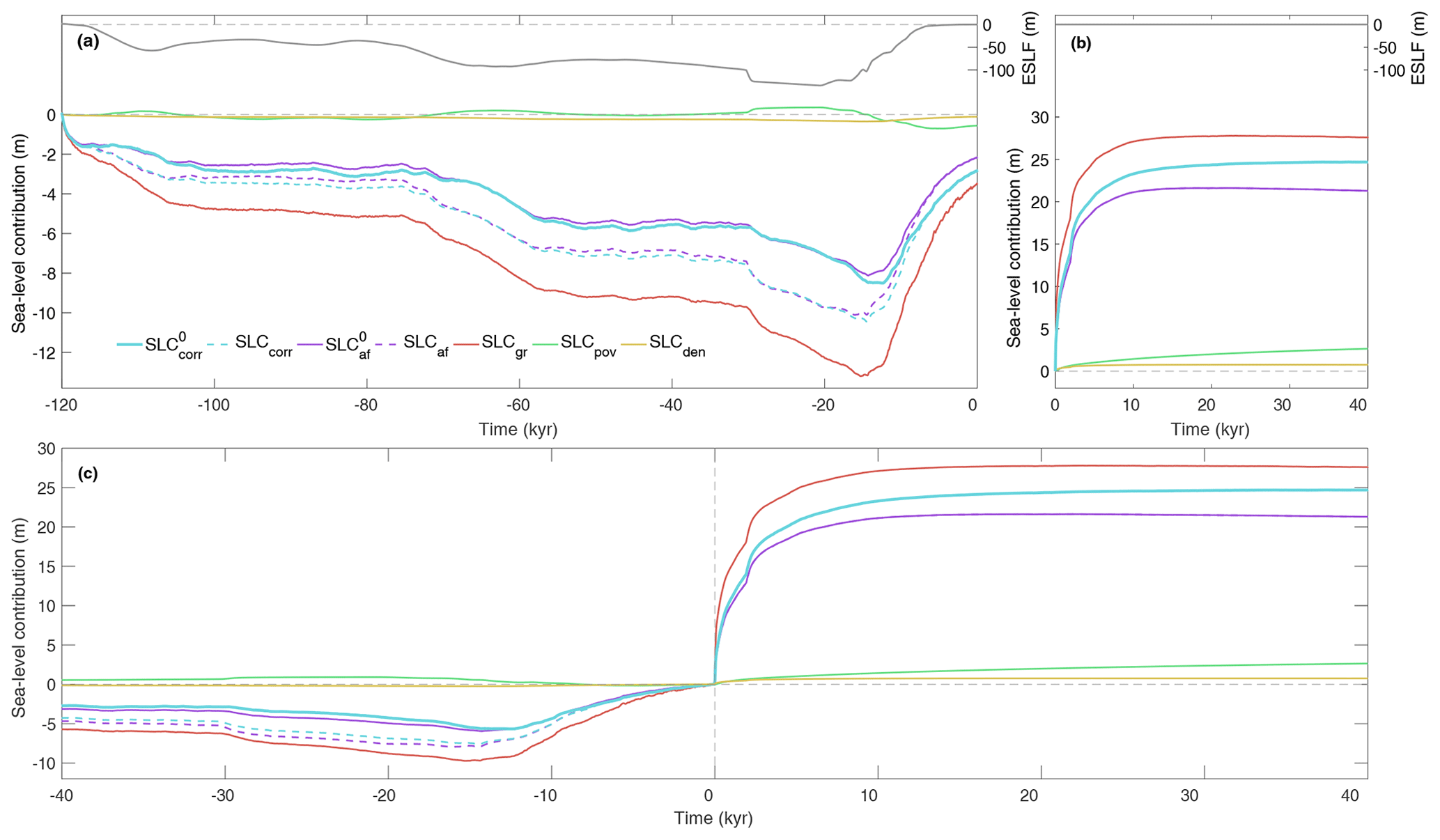
Figure 3Different estimates of the sea-level contribution (SLC) from an Antarctic ice-sheet model simulation. (a) Sea-level contribution for the last glacial cycle under external sea-level forcing (ESLF). (b) Schematic deglaciation experiment over the next 40 kyr in which an extreme sub-shelf basal melt perturbation is applied. The model experiment is continuous across year zero, but estimates in (a) and (b) are referenced to the beginning of each period. (c) Same as (a) and (b) combined, but both experiments are referenced to the present-day configuration. Some lines overlap in (b) and for the future in (c) because ESLF is assumed to be zero for that period. Final corrected sea-level contribution () calculated at constant external reference sea level, based on volume above floatation (), but corrected for potential ocean volume changes (SLCpov) and density (SLCden). The dashed lines (SLCcorr and SLCaf) show results calculated for a variable ESLF (grey lines and left y axis in a and b), and SLCgr is the sea-level contribution when considering all grounded ice without corrections.
Figure 3 illustrates differences in estimated sea-level contributions for an Antarctic ice-sheet simulation with a model that includes a simplified GIA component and external sea-level forcing (Pattyn, 2017). We have first applied a typical glacial–interglacial experiment (e.g. Golledge et al., 2014; Pollard et al., 2016; Albrecht et al., 2020) over the last 120 kyr (Fig. 3a) with the prescribed external sea-level change (based on sea-level reconstructions by Bintanja and van de Wal, 2008, and Lambeck et al., 2014) as a dominant forcing. Atmospheric forcing is produced by perturbing present-day surface temperatures (RACMO2; Van Wessem et al., 2014) with a spatially constant temperature anomaly following ice-core reconstructions from EPICA Dome C (Jouzel et al., 2007), while correcting surface temperatures for elevation changes (e.g. Huybrechts, 2002). The second part of the experiment (Fig. 3b) continues from the present-day configuration and shows the response to an extreme basal melt forcing applied under floating ice shelves. In this schematic forcing scenario, present-day melt rates are multiplied by a constant factor of 200, resulting in melt rates of up to 100 m yr−1 in the Weddell and Ross sea sectors. This extreme melt forcing is not meant to represent a plausible scenario; it only serves to simulate a rapid removal of all floating ice shelves, leading to a retreat of the ice sheet (Pattyn, 2017; Nowicki et al., 2013).
Various SLC corrections and estimates are calculated against the initial configuration in Fig. 3a (120 kyr BP) and against the present-day configuration in Fig. 3b, c. The sea-level contribution calculated from changes in ice volume above floatation (SLCaf) includes signatures of bedrock and (in the past) externally forced sea-level changes. In the future retreat scenario (Fig. 3b), SLCaf is too low compared to our corrected estimate () mainly because ice volume above floatation is “created” by bedrock uplift. This effect of isostatic adjustment on SLCaf is exemplified by the steadily decreasing SLCaf towards the end of the experiment, while remains near constant (due to compensating SLCpov). Accounting for density differences between ocean water and freshwater (SLCden) corrects an additional, but smaller underestimation of SLCaf. The proposed method () is identical to (SLCcorr) for the future period (Fig. 3b), where no external sea-level forcing is applied, and results in an estimate of the sea-level contribution well above SLCaf.
In the paleo-simulation (Fig. 3a), SLCaf is biased by both bedrock changes and external sea-level changes. Since SLCpov is calculated in a fixed domain that includes grounded and floating ice and ice-free ocean areas, it is influenced by ice and ocean water loading. In a glaciation scenario with a growing (Antarctic) ice load and decreasing global sea level (Fig. 3a, before 15 kyr BP), the correction SLCpov is a combination of a subsiding bedrock under the ice sheet (negative SLCpov) and a rising ocean floor in response to reduced water loading (positive SLCpov). We reiterate that the global ocean area Aocean is assumed to be constant here. Although not fully separable, we have estimated the contribution of the two effects by calculating SLCpov within and outside of the glacial ice mask (see Supplement Fig. S1). Both effects are of similar magnitude in our setup, but SLCpov is slightly dominated by the changing ocean floor outside of the ice mask after periods of rapid sea-level forcing change. In addition, during ice-sheet growth, the negative sea-level excursion in SLCaf is exaggerated with increasing amplitude of the external sea-level forcing (compare SLCaf and ). The proposed method () results in an estimate of the negative sea-level contribution in the past of smaller amplitude compared to SLCaf and shows that the magnitude and notably the timing of the Last Glacial Maximum low stand are subject to considerable biases in SLCaf (Fig. 3c). The relative bias in SLCaf is larger for stronger ice-sheet retreat (not shown). Accounting for all grounded ice (SLCgr) would lead in all cases to the largest excursions in negative and positive sea-level contribution, due to ice grounded below the water level that should mostly be replaced by seawater. Differences between the different approaches to calculate SLC become important after 2–3 kyr, roughly corresponding to the shortest response time of bedrock adjustment in the model.
We have presented a unified approach to calculate the sea-level contribution from a marine ice sheet simulated by an ice-sheet model. The formulation notably corrects for changes in ice volume above floatation in the presence of bedrock changes and external sea-level forcing. In this unified approach, sea-level contributions arise from changes in the ice volume above floatation and potential ocean volume, while changes in external sea-level forcing are corrected for.
When bedrock changes in response to ice loading changes occur under ice that is grounded (below sea level), changes in potential ocean volume compensate for changes in ice volume above floatation, resulting in a near-zero net sea-level contribution as should be expected. Under floating ice (or open ocean), changes in volume above floatation are always zero, but bedrock changes imply ocean depth changes that lead to differences in the sea-level contribution (i.e. due to changes in ocean basin volume). The combination of changes in ice volume above floatation and potential ocean volume leads to a generalised formulation that is consistent across changes from floating to grounded ice and vice versa.
The region over which ice thickness changes and potential ocean volume changes are calculated must be fixed in time for the comparison and may contain the entire model grid (as done here) or a reasonable subset. It should include all locations that potentially see ice thickness and/or bedrock changes during a simulation. For models with local isostatic adjustment, the region could be the glacial ice mask for paleo-simulations and the observed present-day sheet-shelf mask for future simulations dominated by retreat. For non-local isostatic models, the footprint would have to be extended.
In all calculations we have ignored any effects that arise from water storage in lakes on land, for example, and we also did not consider the equation of state of seawater, which implies a non-linear dependence of density on salinity and temperature.
The SLC time series in Figs. 3 and S1 are available online at: https://doi.org/10.5281/zenodo.3692702 (Goelzer, 2020).
The supplement related to this article is available online at: https://doi.org/10.5194/tc-14-833-2020-supplement.
HG conceived the project and developed the SLC corrections with assistance of VC. VC performed and analysed the model experiments. HG wrote the manuscript with assistance of all authors.
The authors declare that they have no conflict of interest.
We would like to thank the two reviewers Stephen Price and Rupert Gladstone for their constructive suggestions that helped to improve the manuscript and the editor Ben Galton-Fenzi for guiding the publication process.
Heiko Goelzer has received funding from the programme of the Netherlands Earth System Science Centre (NESSC), financially supported by the Dutch Ministry of Education, Culture and Science (OCW) under grant no. 024.002.001. Violaine Coulon was funded by the Fonds de la Recherche Scientifique de Belgique (F.R.S. – FNRS) with a F.R.S. – FNRS Research Fellowship. Bas de Boer is funded by the SCOR Corporate Foundation for Science.
This paper was edited by Ben Galton-Fenzi and reviewed by Stephen Price and Rupert Gladstone.
Albrecht, T., Winkelmann, R., and Levermann, A.: Glacial-cycle simulations of the Antarctic Ice Sheet with the Parallel Ice Sheet Model (PISM) – Part 1: Boundary conditions and climatic forcing, The Cryosphere, 14, 599–632, https://doi.org/10.5194/tc-14-599-2020, 2020.
Bamber, J. L., Griggs, J. A., Hurkmans, R. T. W. L., Dowdeswell, J. A., Gogineni, S. P., Howat, I., Mouginot, J., Paden, J., Palmer, S., Rignot, E., and Steinhage, D.: A new bed elevation dataset for Greenland, The Cryosphere, 7, 499–510, https://doi.org/10.5194/tc-7-499-2013, 2013.
Bintanja, R. and van de Wal, R. S. W.: North American ice-sheet dynamics and the onset of 100,000-year glacial cycles, Nature, 454, p. 869, https://doi.org/10.1038/nature07158, 2008.
de Boer, B., Stocchi, P., and van de Wal, R. S. W.: A fully coupled 3-D ice-sheet–sea-level model: algorithm and applications, Geosci. Model Dev., 7, 2141–2156, https://doi.org/10.5194/gmd-7-2141-2014, 2014.
de Boer, B., Dolan, A. M., Bernales, J., Gasson, E., Goelzer, H., Golledge, N. R., Sutter, J., Huybrechts, P., Lohmann, G., Rogozhina, I., Abe-Ouchi, A., Saito, F., and van de Wal, R. S. W.: Simulating the Antarctic ice sheet in the late-Pliocene warm period: PLISMIP-ANT, an ice-sheet model intercomparison project, The Cryosphere, 9, 881–903, https://doi.org/10.5194/tc-9-881-2015, 2015.
Goelzer, H.: Dataset for “Brief communication: On calculating the sea-level contribution in marine ice-sheet models” (Version 1), Zenodo, https://doi.org/10.5281/zenodo.3692702, 2020.
Golledge, N. R., Menviel, L., Carter, L., Fogwill, C. J., England, M. H., Cortese, G., and Levy, R. H.: Antarctic contribution to meltwater pulse 1A from reduced Southern Ocean overturning, Nat. Commun., 5, 5107, https://doi.org/10.1038/ncomms6107, 2014.
Gomez, N., Pollard, D., and Mitrovica, J. X.: A 3-D coupled ice sheet – sea level model applied to Antarctica through the last 40 ky, Earth Planet. Sc. Lett., 384, 88–99, https://doi.org/10.1016/j.epsl.2013.09.042, 2013.
Gregory, J. M., Griffies, S. M., Hughes, C. W., Lowe, J. A., Church, J. A., Fukimori, I., Gomez, N., Kopp, R. E., Landerer, F., Cozannet, G. L., Ponte, R. M., Stammer, D., Tamisiea, M. E., and van de Wal, R. S. W.: Concepts and Terminology for Sea Level: Mean, Variability and Change, Both Local and Global, Surv. Geophys., 30, 1251–1289, https://doi.org/10.1007/s10712-019-09525-z, 2019.
Huybrechts, P.: Sea-level changes at the LGM from ice-dynamic reconstructions of the Greenland and Antarctic ice sheets during the glacial cycles, Quaternary Sci. Rev., 21, 203–231, https://doi.org/10.1016/S0277-3791(01)00082-8, 2002.
Jouzel, J., Masson-Delmotte, V., Cattani, O., Dreyfus, G., Falourd, S., Hoffmann, G., Minster, B., Nouet, J., Barnola, J. M., Chappellaz, J., Fischer, H., Gallet, J. C., Johnsen, S., Leuenberger, M., Loulergue, L., Luethi, D., Oerter, H., Parrenin, F., Raisbeck, G., Raynaud, D., Schilt, A., Schwander, J., Selmo, E., Souchez, R., Spahni, R., Stauffer, B., Steffensen, J. P., Stenni, B., Stocker, T. F., Tison, J. L., Werner, M., and Wolff, E. W.: Orbital and Millennial Antarctic Climate Variability over the Past 800,000 Years, Science, 317, p. 793, https://doi.org/10.1126/science.1141038, 2007.
Lambeck, K., Rouby, H., Purcell, A., Sun, Y., and Sambridge, M.: Sea level and global ice volumes from the Last Glacial Maximum to the Holocene, P. Natl. Acad. Sci. USA, 111, 15296, https://doi.org/10.1073/pnas.1411762111, 2014.
Nowicki, S., Bindschadler, R. A., Abe-Ouchi, A., Aschwanden, A., Bueler, E., Choi, H., Fastook, J., Granzow, G., Greve, R., Gutowski, G., Herzfeld, U., Jackson, C., Johnson, J., Khroulev, C., Larour, E., Levermann, A., Lipscomb, W. H., Martin, M. A., Morlighem, M., Parizek, B. R., Pollard, D., Price, S. F., Ren, D., Rignot, E., Saito, F., Sato, T., Seddik, H., Seroussi, H., Takahashi, K., Walker, R., and Wang, W. L.: Insights into spatial sensitivities of ice mass response to environmental change from the SeaRISE ice sheet modeling project I: Antarctica, J. Geophys. Res.-Earth, 118, 1002–1024, https://doi.org/10.1002/jgrf.20081, 2013.
Nowicki, S. M. J., Payne, A., Larour, E., Seroussi, H., Goelzer, H., Lipscomb, W., Gregory, J., Abe-Ouchi, A., and Shepherd, A.: Ice Sheet Model Intercomparison Project (ISMIP6) contribution to CMIP6, Geosci. Model Dev., 9, 4521–4545, https://doi.org/10.5194/gmd-9-4521-2016, 2016.
Pattyn, F.: Sea-level response to melting of Antarctic ice shelves on multi-centennial timescales with the fast Elementary Thermomechanical Ice Sheet model (f.ETISh v1.0), The Cryosphere, 11, 1851–1878, https://doi.org/10.5194/tc-11-1851-2017, 2017.
Pollard, D., Chang, W., Haran, M., Applegate, P., and DeConto, R.: Large ensemble modeling of the last deglacial retreat of the West Antarctic Ice Sheet: comparison of simple and advanced statistical techniques, Geosci. Model Dev., 9, 1697–1723, https://doi.org/10.5194/gmd-9-1697-2016, 2016.
Reerink, T. J., van de Berg, W. J., and van de Wal, R. S. W.: OBLIMAP 2.0: a fast climate model–ice sheet model coupler including online embeddable mapping routines, Geosci. Model Dev., 9, 4111–4132, https://doi.org/10.5194/gmd-9-4111-2016, 2016.
Snyder, J.: Map projections – a working manual (USGS Professional Paper 1395), United States Government Printing Office, Washington, USA, 1987.
van Wessem, J. M., Reijmer, C. H., Morlighem, M., Mouginot, J., Rignot, E., Medley, B., Joughin, I., Wouters, B., Depoorter, M. A., Bamber, J. L., Lenaerts, J. T. M., van de Berg, W. J., van den Broeke, M. R., and van Meijgaard, E.: Improved representation of East Antarctic surface mass balance in a regional atmospheric climate model, J. Glaciol., 60, 761–770, https://doi.org/10.3189/2014JoG14J051, 2014.
- Abstract
- Introduction
- Estimating the sea-level contribution
- Effect of bedrock changes
- Correcting for bedrock changes
- Density correction
- Externally forced sea-level variations
- Ice-sheet modelling example
- Discussion and conclusions
- Data availability
- Author contributions
- Competing interests
- Acknowledgements
- Financial support
- Review statement
- References
- Supplement
The requested paper has a corresponding corrigendum published. Please read the corrigendum first before downloading the article.
- Article
(510 KB) - Full-text XML
- Corrigendum
-
Supplement
(241 KB) - BibTeX
- EndNote
- Abstract
- Introduction
- Estimating the sea-level contribution
- Effect of bedrock changes
- Correcting for bedrock changes
- Density correction
- Externally forced sea-level variations
- Ice-sheet modelling example
- Discussion and conclusions
- Data availability
- Author contributions
- Competing interests
- Acknowledgements
- Financial support
- Review statement
- References
- Supplement