the Creative Commons Attribution 4.0 License.
the Creative Commons Attribution 4.0 License.
 | 02 Dec 2020
Detecting seasonal ice dynamics in satellite images
Alex S. Gardner
Lauren C. Andrews
Fully understanding how glaciers respond to environmental change will require new methods to help us identify the onset of ice acceleration events and observe how dynamic signals propagate within glaciers. In particular, observations of ice dynamics on seasonal timescales may offer insights into how a glacier interacts with various forcing mechanisms throughout the year. The task of generating continuous ice velocity time series that resolve seasonal variability is made difficult by a spotty satellite record that contains no optical observations during dark, polar winters. Furthermore, velocities obtained by feature tracking are marked by high noise when image pairs are separated by short time intervals and contain no direct insights into variability that occurs between images separated by long time intervals. In this paper, we describe a method of analyzing optical- or radar-derived feature-tracked velocities to characterize the magnitude and timing of seasonal ice dynamic variability. Our method is agnostic to data gaps and is able to recover decadal average winter velocities regardless of the availability of direct observations during winter. Using characteristic image acquisition times and error distributions from Antarctic image pairs in the ITS_LIVE dataset, we generate synthetic ice velocity time series, then apply our method to recover imposed magnitudes of seasonal variability within ±1.4 m yr−1. We then validate the techniques by comparing our results to GPS data collected on Russell Glacier in Greenland. The methods presented here may be applied to better understand how ice dynamic signals propagate on seasonal timescales and what mechanisms control the flow of the world’s ice.
- Article
(4526 KB) - Full-text XML
-
Supplement
(7948 KB) - BibTeX
- EndNote


Earth-observing satellites have been in orbit for over half a century, but it was only in 2011 that a sufficient quantity of data had been collected to complete the first pan-Antarctic map of ice velocity (Rignot et al., 2011). Since then, new satellites have led to follow-on mappings that identified regions of changing ice flow (Gardner et al., 2018), and today data are being collected at such a rate that velocity mosaics can be generated every year for nearly all of the world's land ice (Joughin, 2017; Mouginot et al., 2017; Gardner et al., 2019). So for a field of study that was born in an age of in situ stake networks and dead reckoning, the data revolution of the past decade has completely upended glaciology. Where once our challenge was to squeeze as much information as possible from a few sparse field measurements, our biggest challenge now lies in processing massive, often unwieldy datasets and finding all the meaningful signals that lie hidden in this new abundance of data.
One of the most direct and insightful ways to understand how ice moves, what controls its flow, and how it responds to changes in its environment is to observe dynamic variability under a wide range of periodic forcings. Long-term trends and interannual variability (e.g., Moon et al., 2012; Christianson et al., 2016; Greene et al., 2017a; Dehecq et al., 2019) can provide a sense of how glaciers respond to sustained forcing, but on much shorter timescales we are able to see how velocity variations initiate and what physical processes control a glacier's movement. Several targeted studies have shown that glaciers can exhibit observable dynamic responses to ocean tides and that tidal signals can propagate well inland of the grounding line on daily to fortnightly timescales (e.g., Anandakrishnan et al., 2003; Walter et al., 2012; Rosier and Gudmundsson, 2016; Minchew et al., 2017; Robel et al., 2017), but in many glaciers around the world, a significant gap exists in our understanding of how ice dynamic changes develop between tidal and interannual timescales.
It is certainly understood that many mountain glaciers speed up and slow down throughout the year (Burgess et al., 2013; Armstrong et al., 2017; Yasuda and Furuya, 2015; Kraaijenbrink et al., 2016) and that some of Greenland's glaciers respond to seasonal cycles of subglacial hydrology or calving dynamics (Joughin et al., 2008; Howat et al., 2010; Bartholomew et al., 2010; Sole et al., 2013; Moon et al., 2015; King et al., 2018). Seasonal variability has even been reported in a few studies of Antarctic glaciers (Nakamura et al., 2010; Zhou et al., 2014; Greene et al., 2018), but to date, no global-scale mapping of seasonal dynamics of the world's ice has been completed, due in part to the technical challenge of working with optical data in polar regions, where the surface is not touched by sunlight for months-long periods each winter. A comprehensive mapping of the world's seasonal ice dynamics would permit direct intercomparison of seasonal evolution in regions with different driving processes, provide a basis for analysis of long-term changes in seasonal behavior, and supply models with a zeroth-order understanding of global ice dynamics.
In this paper, we describe a precise method of measuring the average seasonal cycle of ice flow dynamics, with the ultimate goal that our method may be used to map the typical magnitude and timing of the seasonal glacier dynamics worldwide. Our study is primarily focused on Antarctica, where seasonal variability is poorly understood and where data limitations currently present the greatest challenges to making such measurements. We test the sensitivity of our method on several thousand synthetic ice velocity time series, then validate it by applying the method to satellite data covering Russell Glacier in Greenland, where we compare our results to GPS observations that show persistent seasonality.

Figure 1Example scenario: (a) shows an ice velocity time series in blue, which integrates to form the cumulative displacement time series shown in (b). We use satellite images to measure ice velocity as the cumulative displacement of crevasses and other glacier features that occurs between acquisition times of any two satellite images. Here, four images taken at times t1 through t4 provide six unique combinations of image pairs that yield the measurements depicted as horizontal gray lines connecting the acquisition times of each image pair. Vertical gray lines show measurement uncertainty, and a black dot is placed at the center times of each image pair for visual clarity. A dashed sinusoid is fit to velocity measurements at the center times of each image pair to highlight the inadequacy of fitting directly to velocity data for determination of seasonal amplitude or phase. This paper describes an alternate, exact approach, wherein sinusoids are fit to accumulated displacements, which are then converted to velocity to produce the light-red velocity sinusoid shown in (a).
The method we present applies to ice velocity datasets such as GoLIVE (Scambos et al., 2016) or ITS_LIVE (Gardner et al., 2019), which have been derived by feature-tracking techniques applied to satellite image pairs. For a detailed review of the principles of feature tracking, we refer readers to Scambos et al. (1992) or Fahnestock et al. (2016), but for the work presented here, it is essential to know only that feature-tracked velocities are measured as the integrated surface displacement that occurs between the acquisition times of two satellite images of a given location. That is, each measurement represents an average velocity between image acquisition dates, and the required passage of time between images precludes direct measurement of instantaneous velocity at any given time. As a result, any high-frequency variability that occurs between images is not represented, and seasonality may appear missing or deprecated in velocity measurements obtained by feature tracking over long time spans (Fig. 1). Nonetheless, by fitting a cyclic function to the time series of displacements rather than average velocities, we show that it is possible to accurately recover the magnitude and phase of seasonal velocity variability.
This paper focuses primarily on the Landsat image pairs that populate the ITS_LIVE dataset, in part because their record extends back as far as 1985 in some locations. The long Landsat record may help ascertain a climatological seasonal cycle of ice dynamics at any given location; however, we face the limitation that optical satellites like Landsat do not collect data throughout the dark winters in polar regions, where land ice is most prevalent (see Fig. 2). Despite the lack of direct observation in winter, we show that the magnitude and timing of seasonal variability can be accurately retrieved from Landsat data, regardless of when in the year the maximum velocity occurs.
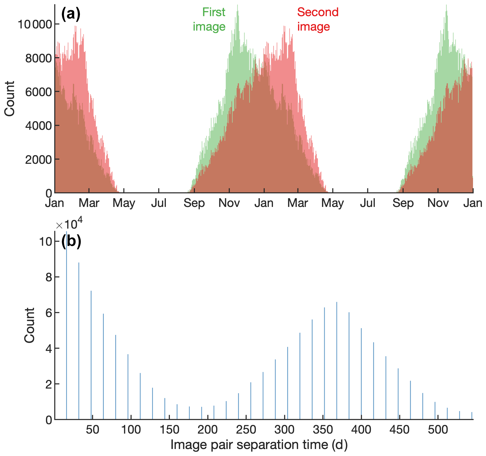
Figure 2Antarctic image pair acquisition times. Over 1.8 million Landsat image pairs provide Antarctic ice velocities in the ITS_LIVE dataset. (a) The seasonal cycle of Landsat image collection shows the effects of the solar cycle on Antarctic sampling. The cycle is repeated for visual continuity over the summer. (b) Displacement fields in the ITS_LIVE dataset are processed for all image pairs separated by 16 to 544 d, with half of all image pairs representing 80 d of displacement or less, but a distinct secondary peak corresponds to a Δt value of 1 year.
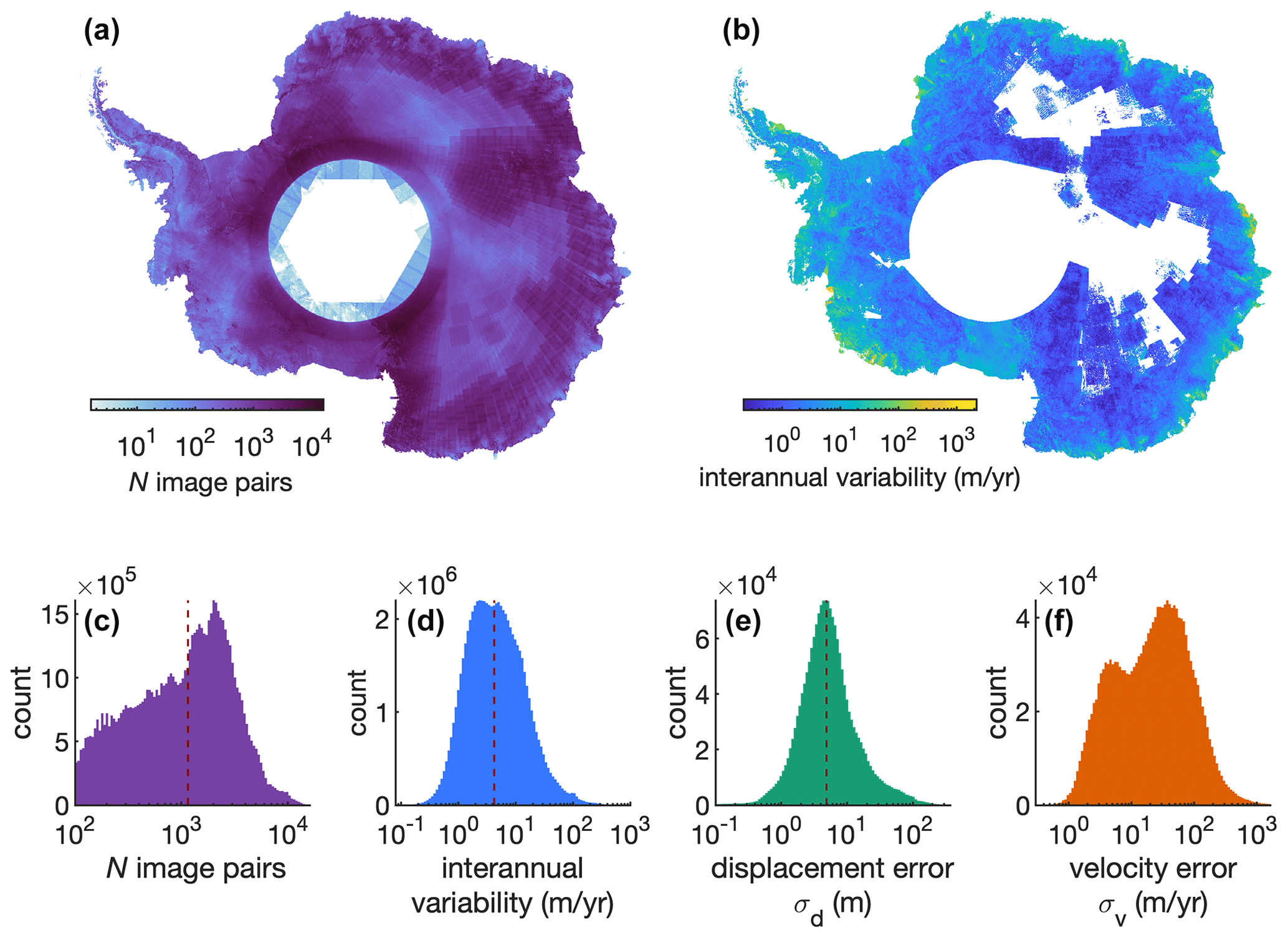
Figure 3ITS_LIVE velocity data statistics. Maps of (a) the number of image pairs that contribute to each 240 m×240 m pixel in the ITS_LIVE summary velocity mosaic and (b) the standard deviation of annual velocity mosaics from 2013 to 2018. Histograms in panels (c) and (d) show only the values from (a) and (b) that correspond to grid cells with at least 100 contributing image pairs and whose mean velocity is at least 15 m yr−1. Displacement errors σd shown in panel (e) result from satellite image georegistration error, and dividing σd by values of Δt corresponding to each image pair results in the velocity errors σv shown in panel (f). Because displacement errors are distributed symmetrically, the bimodal distribution of velocity errors roughly corresponds to the two peaks of Δt values over which velocity is measured (shown in Fig. 2). Vertical lines in panels (c)–(e) indicate median values of 1153 image pairs per grid cell, 4.2 m yr−1 interannual variability, and 4.9 m displacement error.
For any given 240 m×240 m pixel in Antarctica, the ITS_LIVE dataset may contain from a few dozen to more than 10 000 velocity measurements (Fig. 3), which are taken as the ice displacement observed between two satellite images collected on different days. Each satellite image may serve as the first or second image in multiple image pairs, resulting in many overlapping measurements of ice velocity, as shown in Fig. 4. Georegistration error in each image leads to some visible disagreement between the overlapping velocity measurements, but despite the noise, a coherent pattern of interannual variability is apparent as the clusters of velocity measurements move up or down from year to year.
3.1 Assess and remove interannual variability
The first step toward quantifying seasonal variability for any pixel is to remove any interannual variability from the time series. Interannual variability can be determined by smoothing the velocity data using any of several common methods. A polynomial fit is robust and computationally efficient but requires choosing a polynomial order, which is subjective and can lead to overfitting or underfitting the data. Alternatively, a moving average makes no prior assumption about the shape of the velocity curve and can adapt to any arbitrary interannual variability. After exploring several approaches, we find the best results by first detrending the time series with a low-order polynomial, then using a hybrid of a moving average and a spline fit, which we describe below.
When assessing interannual variability, we temporarily ignore the duration over which each image pair measured ice displacement and simply assign the average velocity to the center date tm of each image pair. Using the range of times tm in the time series, we require at least 2 years of velocity data and detrend using a polynomial whose order is chosen as one-fourth of the range of tm in years, rounded up to the nearest integer. The result is that for up to 4 years of data, the time series is linearly detrended; from 4 to 8 years of data, the time series is quadratically detrended, and so on. We assign the velocity weights wv in the polynomial fit using the formal error estimates σv from the ITS_LIVE data product such that . An example of a fourth-order polynomial fit to the velocity data is shown in Fig. 4.
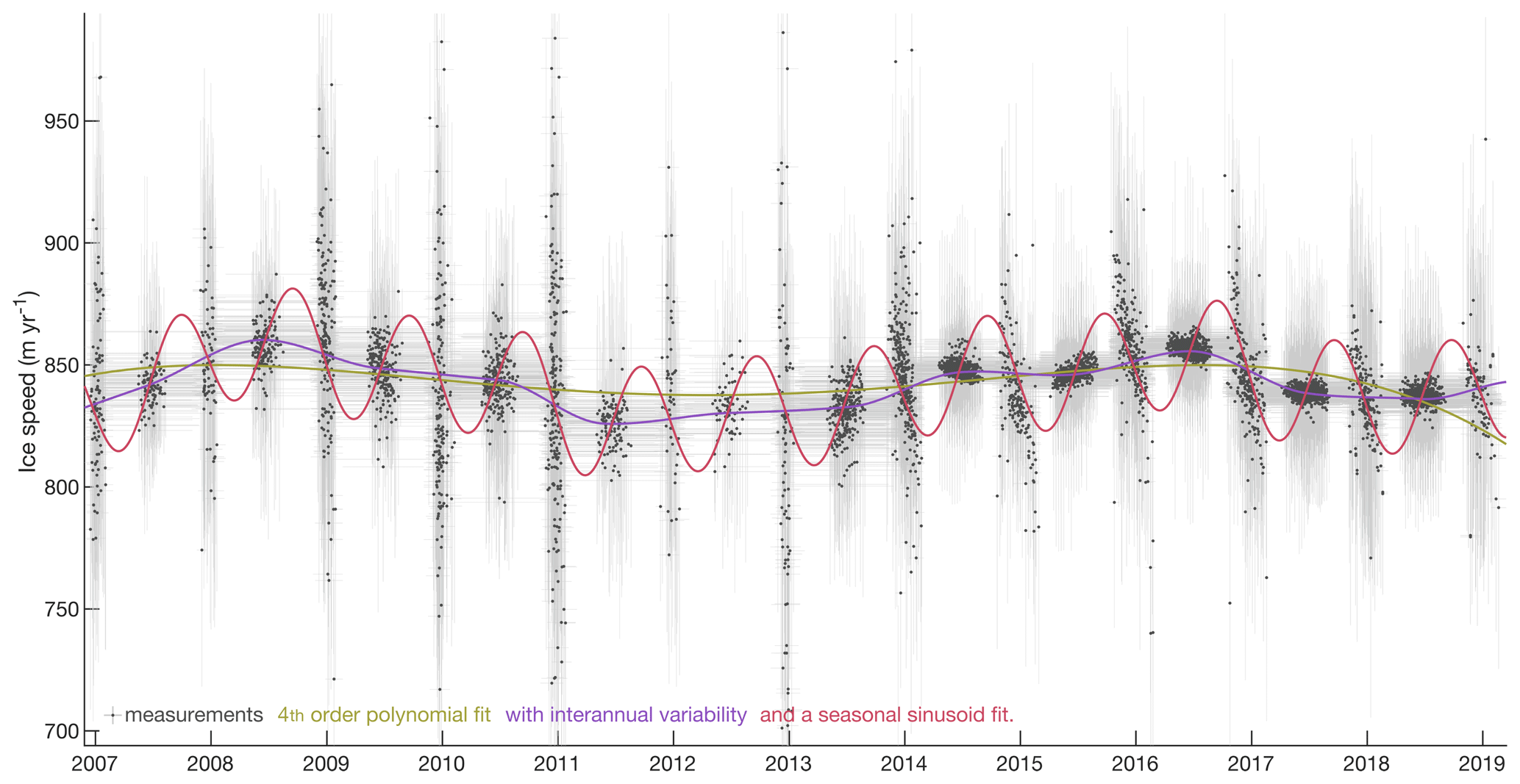
Figure 4Velocity time series for an ITS_LIVE pixel. The clustering of these 14 208 measurements taken near the grounding line of Byrd Glacier typifies ITS_LIVE image pair data, with short-Δt measurements providing direct but noisy observations of velocity variability throughout each summer, while much lower-noise winter estimates can only give insight into the total displacement that occurs during the dark, winter months. Light-gray horizontal bars connect the acquisition times of each image pair, and vertical bars show ±1σv uncertainty. Center dates tm are shown as dark-gray dots for visual clarity.
After detrending the time series with a weighted polynomial fit, we characterize any residual interannual variability with a spline fit to the mean velocities of each year. We take the weighted mean velocity of all measurements whose tm lies within 183 d of winter solstice of that year. We assign the weighted mean velocity of each year to the weighted mean date of those velocities, then interpolate with a shape-preserving piecewise cubic hermite polynomial to obtain a measure of interannual variability corresponding to each image pair's center date tm.
In the method described thus far, most summer image pairs whose Δt is small contribute much less to the weighted mean annual velocities than do long Δt image pairs that span winter. This is because velocity error by any feature-tracking algorithm stems strictly from displacement error σd, while timing error is essentially 0. So although summer offers more image pair measurements, their shorter Δt values are associated with greater velocity error σv, and therefore they are significantly down-weighted in the calculation of annual mean velocities. In other words, it is possible that due to either the higher weights of winter velocities or the higher quantity of measurements available during summer, the weighted mean annual velocities could be biased toward one season or the other. We account for this possibility by iteratively solving for interannual and seasonal variability, as we describe later in Sect. 3.3.
3.2 Assess seasonal variability
We characterize the magnitude and timing of seasonal variability as a simple sinusoid that can be applied in the x and y directions separately to build a two-dimensional understanding of how ice moves throughout the year. Limitations of the sinusoidal approximation are discussed later in Sect. 6, but we justify our approach as it is the simplest means of describing cyclic behavior, and by nature it is constrained to capture the sum total of ice displacement that occurs throughout the year.
After characterizing interannual variability, we subtract it from the velocity time series at the center date of each image pair. The residuals vr after removing interannual variability can then be assumed to contain only seasonal variability and noise. To address blunders, we remove outliers whose absolute value exceeds 2.5 robust standard deviations of vr (see Appendix A). The remaining task is to fit a sinusoid to the vr time series, but given that each velocity measurement is a single value that represents several weeks to more than a year, we cannot fit a sinusoid directly to the velocity time series or assume that values of vr correspond to the image pair center dates tm. Instead, we operate on the displacements associated with each image pair, taken as the integrals of velocities vr.
We seek to define seasonal velocity variability vs in the form
where A and ϕ are the amplitude and phase of the seasonal velocity cycle, respectively; t represents time in decimal years; and T=1 year is the period of oscillation. By our method, the constant C0 is ideally 0 after detrending and removing interannual variability, but we include it here in case some residual offset is present in the vr time series.
For a more robust least-squares solution, we employ a trigonometric identity to rewrite Eq. (1) as
which is related to Eq. 1 by and .
Again, we cannot solve Eq. (1) or Eq. (2) directly with image pair velocities because they do not represent instantaneous velocity at any known times t. Instead, image pair data track displacements, which equate to the integral of velocities between times t1 and t2 when the two images were acquired. Accordingly, we can take the definite integral of Eq. (2) to solve for the seasonal displacement cycle ds as
We solve for the coefficients of Eq. (3) using a least-squares approach with weights given by . This type of approach has previously been applied to study Earth deformation (e.g., Hetland et al., 2012) and is similar to an approach that has been used to analyze ice dynamic responses to tidal forcing (Milillo et al., 2017; Minchew et al., 2017).
By employing Eq. (3) to solve for A and ϕ, we obtain a first approximation of the seasonal variability in ice velocity. However, the possibility remains that the initial estimate of interannual variability may have been partly aliased by seasonal variability due to uneven temporal sampling. Thus, we refine our estimates of interannual and seasonal variability by iterative means.
3.3 Iteratively refine interannual- and seasonal-variability estimates
If our first estimates of A and ϕ are correct, then seasonal variability must have aliased each initial estimate of interannual variability by a certain amount va. The amount of velocity aliasing equates the seasonal displacement over time, which we can obtain by dividing the definite integral of Eq. (1) by Δt, or
After obtaining initial estimates of A and ϕ, we subtract va from the original detrended velocity measurements and repeat the process of calculating interannual and seasonal variability. In most cases, we find that initial estimates of A and ϕ are reasonably close to their true values and that just a few iterations are sufficient to yield accurate final estimates of seasonal amplitude and phase. We explore the number of requisite iterations in Sect. 4.3 and show the effects of iterating in Fig. 5.
Figure 4 shows an example of our method applied to a time series of 14 208 ITS_LIVE image pairs acquired in a single pixel near the grounding line of Byrd Glacier, Antarctica. Because no strong long-term velocity trends are present, the green fourth-order polynomial fit is relatively flat, albeit with a slight downturn at the unconstrained end of the time series. The blue curve of interannual variability follows the multiyear rises and falls of velocity much more closely and is uncontaminated by seasonal variability on this 10th iteration of the solution. The red curve adds seasonal variability with an amplitude of 23 m yr−1 to the interannual variability, and given that it is a least-squares solution, it represents the only solution that minimizes the misfit between the curve and all available observations. Indeed, while at first glance it may appear visually that the timing of image acquisitions themselves is the only seasonal pattern in the ITS_LIVE data plotted in Fig. 4, close inspection shows a persistent pattern of summer slowdown in the image pair data that becomes especially clear after the 2013 launch of Landsat 8.
To assess uncertainty in our method, we generate synthetic random continuous velocity time series, then artificially sample them using random subsets of image acquisition times from Landsat image pairs that cover Antarctica. We then apply the methods described in Sect. 3 to determine how accurately seasonal ice dynamics can be measured and under what conditions.
4.1 Synthetic time series generation
Any synthetic velocity time series used for testing should resemble the true nature of ice dynamics in its variability on all timescales. Accordingly, we create realistic interannual variability by matching the distribution of the standard deviations of velocities in each grid cell in the ITS_LIVE annual velocity mosaics from 2013 to 2018. Figure 3 shows a map of interannual variability for the grid cells that contain all 6 years of data and a histogram of those values for grid cells that contain at least 100 total image pairs and a minimum mean velocity of 15 m yr−1. Within this subset, the median interannual variability is characterized by a standard deviation of 4.2 m yr−1.
To create each synthetic time series of interannual variability, we generate uniformly distributed random values centered about 0 at daily temporal resolution. We apply a first-order low-pass Butterworth filter with a cutoff period of 548 d to each random time series to ensure that no annual cycles are present, and then we discard the first and last 548 values of each time series to eliminate edge effects of the filter. We then scale the remaining time series such that its standard deviation matches a prescribed level of interannual variability.
Our handling of interannual variability is an attempt to mimic the observable ways in which Antarctic glaciers speed up and slow down from year to year. Ideally, we would also carry forth in a similar manner for seasonal variability, imposing cyclic behavior that matches the true character and distribution of the types of seasonal variability that exist in nature. However, as the intent of this paper is to develop the methods that will be necessary to understand where and how ice velocities vary on seasonal timescales, we cannot at present create synthetic seasonal-variability distributions to match what truly exists in nature. Instead, to each synthetic time series we add a sinusoid with a period of 365.25 d, a random phase, and a random amplitude between 0 and 100 m yr−1.
4.2 Synthetic time series sampling
Each synthetic time series is artificially sampled using characteristic acquisition times and error distributions from Antarctic Landsat-derived ITS_LIVE image pairs. In Fig. 3 we see that among grid cells containing at least 100 image pairs and whose mean velocity is at least 15 m yr−1, we can expect a median of 1153 image pairs per grid cell. Accordingly, we use the acquisition times (Fig. 2) and corresponding error estimates (Fig. 3) from random subsets of 1153 image pairs (sampled from all 1.8 million Antarctic image pairs) to artificially sample each synthetic time series. Each synthetic velocity measurement is calculated from the cumulative sum of daily velocities that occurred between the first and second image in a given pair, but before dividing the total displacement by the time Δt between images, a random Gaussian value of displacement is added according to the formal error estimates associated with that image pair in the ITS_LIVE dataset. The result is a time series of synthetic measurements that resemble the acquisition times and error characteristics of ITS_LIVE image pairs but whose underlying continuous velocity signal it represents is known.
Table 1Sensitivity test parameters. To understand how various factors influence measurement sensitivity, we isolate and vary a number of key characteristics of the synthetic time series and the data analysis method. In the first test, we vary only the number of iterations described in Sect. 3.3 to determine how many iterations are necessary to achieve a stable solution. We then test the effects of sampling velocity time series with 32 to 10 000 synthetic image pairs. In the remaining tests, we prescribe characteristics of the synthetic velocity time series to understand the influence of interannual variability, the amplitude of the seasonal cycle, and the timing of the seasonal cycle on measurement accuracy.
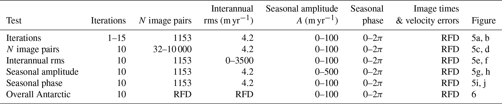
RFD indicates randomized from distribution of all 1.8 million Antarctic ITS_LIVE image pairs.
4.3 Seasonal amplitude and phase recovery
We conducted several tests to determine the accuracy with which we can recover the amplitudes and phases of seasonal cycles in synthetic velocity time series. The parameters of each test are detailed in Table 1.
In the first test, we sought to understand how many iterations are necessary to achieve a stable solution. In this test, we generated 10 000 synthetic velocity time series, each having interannual variability with a standard deviation of 4.2 m yr−1. Sinusoidal seasonal variability was added to each time series, characterized by a random phase and a uniform distribution of amplitudes between 0 and 100 m yr−1. Each time series was then synthetically sampled using the acquisition times and error characteristics of 1153 random image pairs in the ITS_LIVE dataset. Following the method described in Sect. 3, we analyzed each time series by assessing interannual variability in the synthetic measurements, removing it, removing outliers, and then obtaining the amplitude and phase of each seasonal cycle. After accounting for any aliasing that would have been caused by the seasonal amplitude and phase (Sect. 3.3) that were measured in the first iteration, we conducted a second iteration of assessing interannual and seasonal variability. We then followed with a third iteration, and so on, up to 15 iterations. Results in Fig. 5a and b show that solutions tend to converge after the first few iterations, but it is possible that in some situations more iterations could be necessary, depending on sampling and the characteristics of the velocity time series. Accordingly, we use 10 iterations in all of the tests that follow.

Figure 5Sensitivity test results. The tests outlined in Table 1 indicate that (a, b) amplitude and phase errors level off after the first few iterations of removing interannual variability and solving for seasonal variability; (c, d) at least 500 to 1000 image pairs are necessary for the most accurate, stable solutions; (e, f) strong interannual variability can drastically affect seasonal amplitude and phase detection; (g) seasonal-amplitude measurement uncertainty is independent of the seasonal ice velocity amplitude itself, but (h) seasonal phase is measured most accurately when the seasonal ice velocity amplitude is strong; and (i, j) although some faint residual effects of the seasonal bias in sampling persist after 10 iterations, amplitude and phase accuracy are effectively independent of the timing of the seasonal ice velocity variability.
We conducted a second test to determine how many image pairs are necessary to detect seasonal cycles in a velocity time series. We found that with just 32 image pairs, we were able to recover phase with sufficient accuracy to correctly identify the season of maximum velocity (Fig. 5c, d). We also found that performance improves dramatically with increasing image pairs until errors in phase and amplitude approach their asymptotes, between 500 and 1000 image pairs. Beyond that, the number of image pairs used in the analysis has a negligible impact on the accuracy of seasonal signal detection.
In a third test, we found that one factor more than any other threatens the accuracy of seasonal-variability detection. Given a velocity time series sampled by 1153 image pairs, seasonal-amplitude error increases approximately linearly with the level of background interannual variability (Fig. 5e, f). This is because despite our attempts to account for interannual variability, it is inevitable in a time series of finite length that some residual variability will influence the least-squares fit of the seasonal cycle. Nonetheless, if we consider ±45 d of phase uncertainty to be a threshold that indicates accurate detection of the season of maximum velocity, our method performs adequately in the presence of interannual variability with a standard deviation exceeding 100 m yr−1. Further analysis suggests that for any level of interannual variability, the amplitude of the seasonal cycle must be at least one-third of the standard deviation of interannual variability to reliably be detected (see Sect. A1). We note, however, that because we have used the simple metric of the standard deviation of velocity to describe all forms of interannual variability, it is likely that our method will perform better than these error estimates suggest wherever interannual variability is dominated by a long-term trend.
The final four panels (g–j) of Fig. 5 provide valuable insights into the capabilities and sensitivities of our seasonal detection method, most notably that, for a constant level of background interannual variability, seasonal-amplitude errors are independent of the amplitude of the seasonal cycle. However, phase detection benefits with increasing seasonal amplitude. This should not be surprising as a signal must not only exist but also be sufficiently strong for its phase to be accurately measured. The last two panels (i–j) of Fig. 5 show that for all practical purposes our seasonal amplitude and phase estimates can be considered insensitive to the timing of the underlying seasonal signal, despite having no images during winter.
Thus far we have determined that 10 iterations are more than sufficient for the model of seasonal variability to converge. We have also found that our measurements can be considered agnostic to the timing of ice velocity variability and to the timing of satellite image acquisitions when applied to at least 500 to 1000 image pairs. With this understanding, we now apply our method to 100 000 synthetic time series that typify the interannual ice velocity variability and satellite image acquisitions that have been measured across the Antarctic continent as a whole. Interannual variability in the synthetic time series was randomly sampled from the distribution shown in Fig. 3d, and a uniform distribution of seasonal amplitudes from 0 to 100 m yr−1 was added to the interannual variability. Each synthetic ice velocity time series was observed with a number of synthetic image pairs taken randomly from the distribution of values in Fig. 3c that exceed 500 image pairs, and displacement errors randomly sampled from the distribution in Fig. 3e were added to each synthetic measurement before dividing by the times Δt that separate each image pair. The results of this test, shown in Fig. 6, indicate that with the Landsat images that have been acquired to date, we should be able to measure seasonal amplitudes within ±1.4 m yr−1 and phase within about ±2 d.
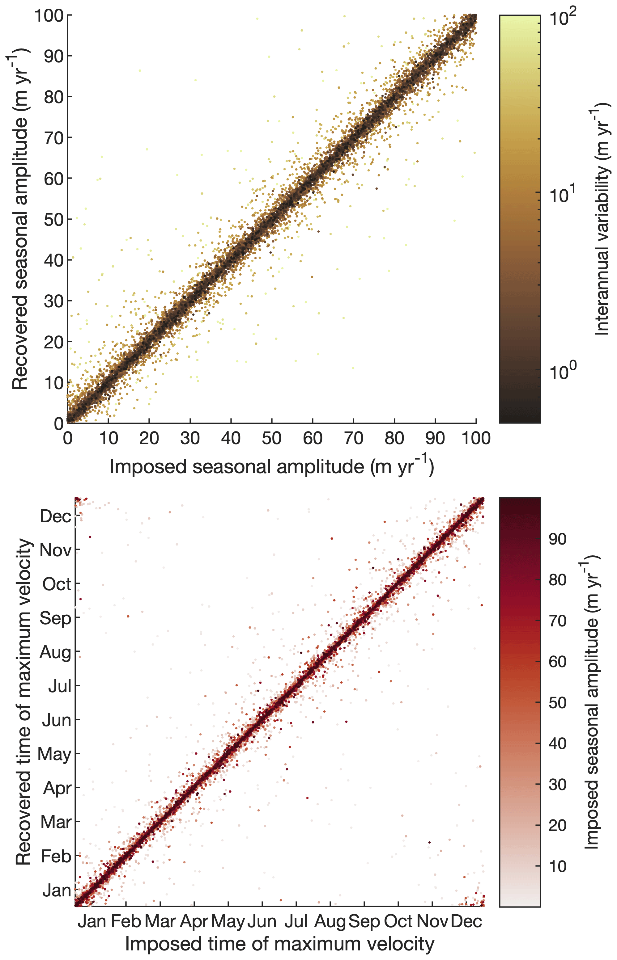
Figure 6Pan-Antarctic seasonal signal recovery. Following the parameters of the final test in Table 1, we examine the performance of our method using the complete distributions of Antarctic Landsat image acquisition times, ITS_LIVE velocity errors, and measured Antarctic interannual ice velocity variability. Among the results where 500 or more image pairs were used to analyze the time series, amplitude uncertainty was found to be 1.4 m yr−1, and phase uncertainty is 2 d visual clarity. Only 10 000 randomly selected results are shown of the 100 000 tests we performed for overall Antarctic parameter distributions.
To confirm that we can extract seasonal ice velocities from feature-tracking data, we compare an in situ GPS position time series against results obtained by applying our method to ITS_LIVE velocities that were generated from 15 m resolution optical Landsat 7 and 8 imagery. We focus on Russell Glacier in Greenland, where GPS data provide more than a decade of observations and where seasonal velocity variability has previously been reported (Van de Wal et al., 2015). We use the GPS-derived positions from the Programme for Monitoring of the Greenland Ice Sheet (PROMICE; Van As, 2011) KAN_L station (67.0960∘ N, 49.9433∘ W; 673 m a.s.l.; see Appendix B). Although we ultimately aim to characterize Antarctic seasonality, we use this record from Greenland because we are not aware of any such decade-long GPS records in Antarctica that offer winter position data and capture seasonal cycles of glacier movement that can be used for validation. The ITS_LIVE data covering Greenland are identical to the Antarctic image pair data, so we directly apply the methods discussed above without any adjustments. Likewise, our methods could just as easily be applied to ITS_LIVE data covering Alaska, the Canadian Arctic, Svalbard, the Russian Arctic, Patagonia, or High Mountain Asia.

Figure 7GPS validation at Russell Glacier, Greenland. Hourly time series of (a, b) detrended positions of a GPS receiver are shown as raw data in light blue and the sum of interannual variability and a sinusoid fit in dark blue. The amplitudes of positional seasonal variability are only 4.5 m in the easting (x) direction and 1.8 m in the northing (y) direction, yet these minor seasonal displacements are easily detected by applying the methods described in Sect. 3 to ITS_LIVE Landsat image pair velocities. (c, d) Velocity measurements from 5189 ITS_LIVE image pairs are plotted in gray, with our fit to the measurements in red. The blue velocity curves are simply the time derivatives of the corresponding GPS position curves plotted in panels (a) and (b). The level of agreement between the two independent measurements is detailed in Table 2.
Figure 7a and b show the linearly detrended GPS position data along with a model fit that represents the sum of interannual variability and a seasonal sinusoid fit to the position data (see Appendix B). From the GPS data, we obtain velocity time series by taking the time derivative of the position fits, which are shown in Fig. 7c and d. As we expect when taking the derivative of a sinusoid, the peaks in velocity occur 91 d before peaks in position, and velocity amplitudes are 2π yr−1 times the amplitudes of the seasonal position fits.
We compare the GPS velocity time series to velocities obtained from 5189 ITS_LIVE image pairs in the pixel closest to the fixed median location of the GPS receiver throughout the course of its data collection. Key findings are listed in Table 2. Secular mean velocities in the x and y directions measured by the two independent datasets agree on the order of 1 m yr−1. Seasonal velocity amplitudes also show agreement on the order of 1 m yr−1, as we expect on this glacier, where interannual variability has a standard deviation of 3.6 m yr−1 in the x direction and 3.4 m yr−1 in the y direction (see Appendix A2).
Table 2ITS_LIVE analysis compared to GPS. The secular mean velocities and x and y components of the seasonal characteristics of the glacier velocity time series shown in Fig. 7. The acquisition dates of the two independent measurements differ slightly, yet agreement is within a few percent by every measure. Uncertainty estimates are described in Appendix A2.
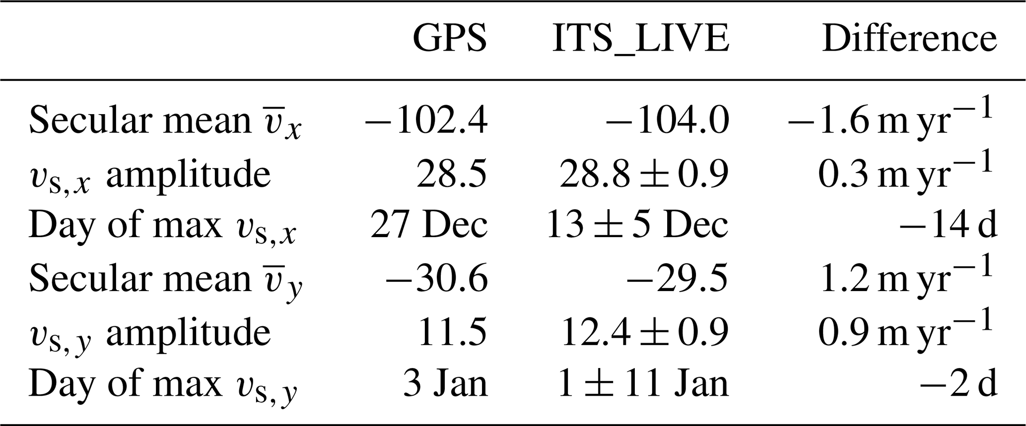
The largest disagreement in Table 2 lies in the phase of the x direction, which at 14 d is only about 4 % of a year. We note further that disagreements listed in Table 2 do not necessarily reflect errors in the ITS_LIVE data or the methods we have employed to process it. Rather, disagreements may simply reflect that the GPS receiver did not record data from late 2010 to mid 2012, and no GPS data were recorded during two of the winters that followed. Meanwhile, we use ITS_LIVE data from images that were collected more than a year before the start of the GPS record, but image pair data have not yet been processed corresponding to the final months of the GPS record. In addition to these differences in timing of data collection, we also note that the GPS record represents a Lagrangian measurement of ice velocity, whereas the ITS_LIVE data record an Eulerian measurement at a pixel that the GPS receiver passed through only once in its decade-long life. Nonetheless, agreement between the GPS solutions and our method of image pair data analysis is notable and lends credence to this method as a precise means of measuring seasonal variability in ice velocity.
The method we present in this paper requires a multiyear record with at least several hundred image pairs to confidently identify the amplitude and phase of seasonal variability. Some key regions of interest, such as Totten Glacier in Antarctica, do not yet offer enough cloud-free images to meet this threshold, so a few more years of data collection may be required before our methods can be successfully implemented there. In addition, it may be difficult or impossible by our methods to detect seasonality in places of interest such as Pine Island and Thwaites glaciers, which are currently undergoing dramatic interannual change (Mouginot et al., 2014) that could confound our measurements of seasonal variability.
Nonetheless, Fig. 7 illustrates the sensitivity of our method to tiny variations in glacier flow when conditions are favorable. The vertical scale of the upper panels spans just ±15 m; yet, by our method of analyzing 15 m resolution Landsat Band 8 images, we are able to detect minor nuances in position that occur entirely within this range. We know of no other sensor or dataset that can offer such insights into these kinds of subtle variabilities in ice flow that have occurred over the past few decades.
The most significant limitation of the method we present may lie in our approximation of seasonal variability as a sinusoid. Where seasonal dynamic variability has previously been documented, it has been found that in some cases a sawtooth function or other higher-order fits might match seasonal variability more closely than a sinusoid (Moon et al., 2014; Van de Wal et al., 2015; Vijay et al., 2019). In particular, although events such as springtime calving or summer melt may occur on an annual cycle, a glacier's complete response to them may only last for only a few days (Schoof, 2010). Approximating such events as smoothly varying sinusoids will underestimate the magnitude of any brief glacier acceleration while potentially giving a false sense that the ice responds to an impulse event continually throughout the entire year.
Despite the tendency of a sinusoid to oversimplify complex time series, we contend that no other description of seasonal variability is as elegant or robust over decadal timescales and that understanding seasonal ice dynamics must begin with a zeroth-order description of the amplitude and phase of ice velocity variability. While it is true that a glacier can accelerate in response to a transient event and return to an equilibrium velocity within just a few days (Stevens et al., 2015; Andrews et al., 2014), in the climatological sense, nature does not consistently time such events as calving or increases in basal water pressure with any greater precision than the method we have presented to detect them. Short-lived speedup events do not consistently occur on the same day each year, so the decadal average tends to be smoother and more sinusoidal than the velocity profile of any single year.
The approach we present captures the fundamental mode of subannual variability in ice velocity and conserves all ice displacement that occurs throughout the year. The simple two-term explanation of amplitude and phase provides a robust description of seasonality that is less prone to error than higher-order fits such as three-term sawtooth functions. By providing a simple measure of amplitude and phase, we offer a straightforward method to compare how neighboring glaciers respond to a common seasonal forcing or investigate how dynamic signals propagate upstream or downstream in a given glacier.
In Sect. 5 we apply our method to ITS_LIVE velocity measurements and compare against GPS position data with the intention that the in situ GPS station would provide a reliable ground-truth reference. However, although the two independent measurements show close agreement whenever GPS data were logged, the receiver's harsh polar environment has led to several long gaps during which no GPS position data were acquired. This suggests that, as a means of measuring ice dynamic climatology, our method might not only meet but exceed the performance of the in situ GPS receiver while providing insights into dynamic behaviors that occurred years before the station was installed. The particular ITS_LIVE grid cell in Greenland that we analyzed in this paper is hardly unique in its potential to provide historical context as decades-long velocity records exist in most of the 240 m×240 m pixels, which cover nearly all of the world's ice.
The methods presented in this paper have focused primarily on optical satellite data because no other type of sensor provides such a long record of ice velocity. As more radar data become available, particularly since the launch of Sentinel 1a/b, the problem of missing winter data will be eliminated, but the methods presented in this paper will still hold. When an abundance of feature-tracked velocities from radar become available, Eq. (3) may then be easily modified to include additional terms to simultaneously solve for cyclic velocity variability on tidal timescales as well as seasonal variability.
Given a relatively continuous time series of at least 500 to 1000 image pairs, our method can extract the amplitude of seasonal variability with a precision on the order of about 1 m yr−1 by describing ice flow as an oscillation, provided the level of background interannual variability does not overwhelm the overall signal. We find that if the amplitude of seasonal variability is at least a third of the standard deviation of interannual variability, the method we describe can reliably detect the season of maximum ice velocity. Ability to detect seasonal amplitudes is independent of the amplitude and phase of the seasonal velocity variability, but phase accuracy benefits with increasing amplitude of seasonal variability.
With the method we describe, we may begin to map seasonal ice dynamic variability on a global scale in a consistent and meaningful manner, and by providing a method that can be employed independently in the two dimensions of Cartesian coordinates, we hope to gain a more complete understanding of how dynamic signals propagate through the world's ice.
Phase and amplitude uncertainty in Sect. 4.3 were calculated from the differences between imposed and recovered values. Differences in phase were wrapped such that their absolute values did not exceed 182.62 d. During this work, we found that in some cases, simple standard deviations of differences could be strongly influenced by a few extreme outliers, and as a result, standard deviations of differences (and similarly, root-mean-square errors) did not reflect the true Gaussian distributions of errors. So for a more robust and meaningful measure of error distributions, we define σ as 1.4826 times the median of the absolute value of differences.
A1 Seasonal uncertainty from interannual variability
In addition to the tests described in Sect. 4.3, we analyzed 120 000 synthetic time series to better understand the scenarios in which interannual variability may confound our ability to detect seasonal cycles in an ice velocity time series. For every unique combination of 31 values of seasonal amplitudes from 0 to 1000 m yr−1 and 26 values of interannual variability from 0 to 3500 m yr−1, we generated 150 synthetic time series, sampled them with 1153 synthetic image pairs, and attempted to recover the seasonal cycles we imposed. A striking relationship emerged, shown in Fig. A1, in which we see a strong demarcation between a zone of accurate phase detection and a zone where phase cannot be determined with any confidence.
Letting phase uncertainty of 45 d be the threshold indicating whether the season of maximum ice velocity can be accurately determined, in Fig. A1 we see that above the noise floor of about 1 m yr−1 seasonal amplitude, the 45 d phase uncertainty contour marks an approximately linear relationship between interannual variability and seasonal amplitude. Indeed, the dashed blue line that nearly coincides with the 45 d phase uncertainty contour shows the simple slope, whereby seasonal amplitude is one-third of the standard deviation of interannual variability, with zero offset from the origin. This tells us that there is a quite simple relationship between the amplitude of a seasonal cycle, the level of background interannual variability, and our ability to detect phase. As long as the seasonal amplitude is above the noise floor of about 1 m yr−1, and interannual variability does not exceed 3 times the amplitude of the seasonal cycle, we can accurately detect the seasonal cycle.
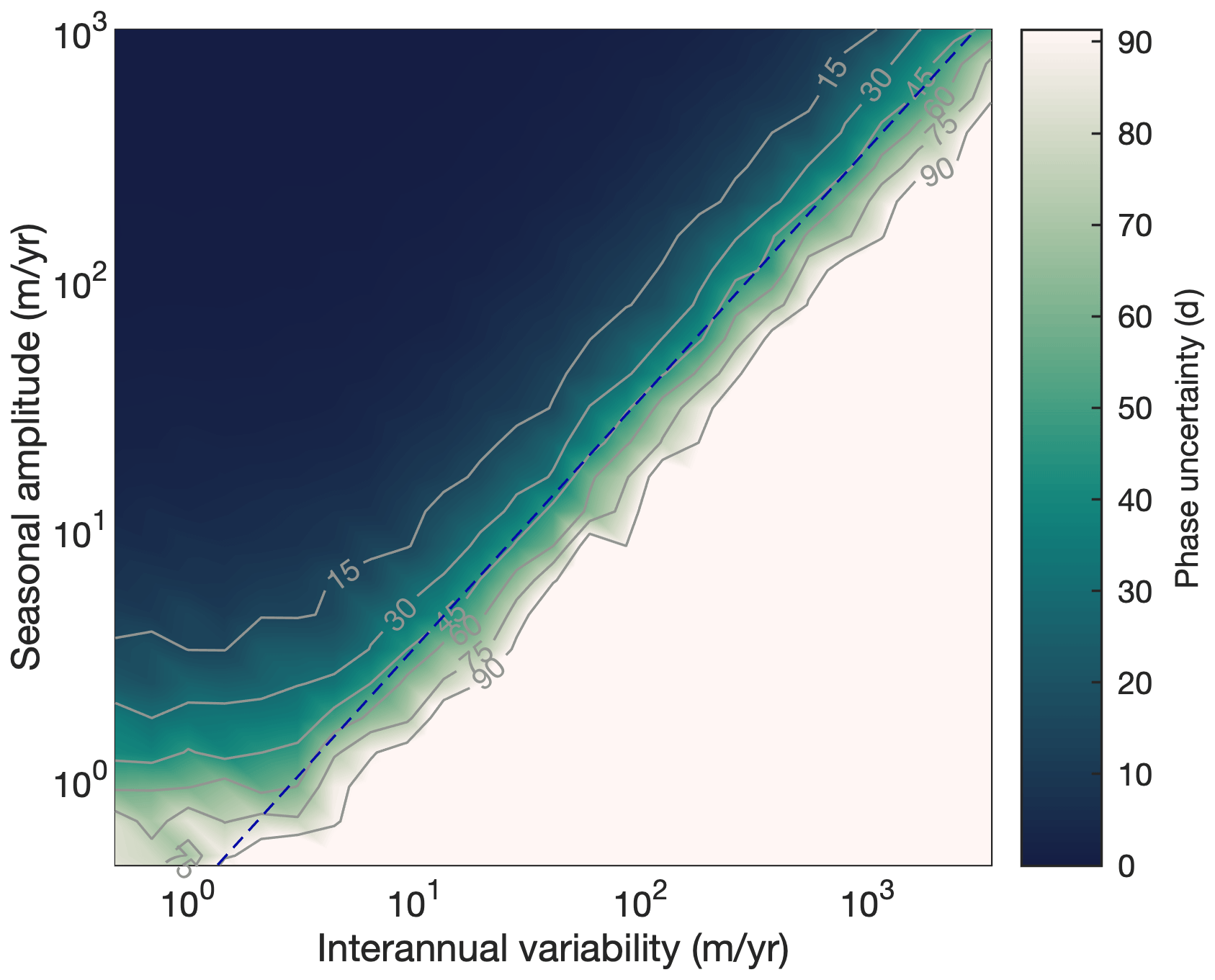
Figure A1Interannual variability and seasonal signal detection. The dark-green region of this plot indicates scenarios in which phase can be accurately detected with 1153 image pairs. When seasonal amplitudes are above the noise floor of about 1 m yr−1, the amplitude of seasonal variability must be at least a third of the standard deviation of interannual variability to be detected, and this relationship is marked by a dashed blue line. The linear relationship coincides with the 45 d phase uncertainty contour that determines whether the season of maximum ice velocity can be accurately measured.
A2 Uncertainty estimates for comparison of ITS_LIVE to GPS
The values of seasonal amplitude and phase uncertainty listed in Table 2 were each calculated as the robust standard deviations of amplitude and phase errors from 5000 synthetic time series sampled by 5189 image pairs. In the x direction, ITS_LIVE image pairs indicate an interannual variability of 3.85 m yr−1 in our pixel of interest, with a seasonal amplitude of 28.8 m yr−1 and a maximum velocity occurring around 13 December of each year. We generated 5000 synthetic time series matching these criteria and were able to recover the 28.8 m yr−1 seasonal amplitude within σ=0.87 m yr−1 and phase within σ=4.7 d. Similarly for the y direction, from 5000 synthetic time series with an interannual variability of 3.38 m yr−1, seasonal amplitude of 14.4 m yr−1, and maximum velocity occurring on 1 January of each year, we recover seasonal amplitudes within σ=0.91 m yr−1 and phase within σ=10.7 d.
We use hourly position data from the PROMICE KAN_L GPS station on Russell Glacier (Van As, 2011).
The KAN stations utilize the Trimble SAF270-G antenna with a single L1 frequency to minimize power usage. L1 signals have previously been used in studies of short-term ice motion with success in the Russell Glacier region (e.g., Van de Wal et al., 2015). Positions are recorded hourly during the spring–summer observation period and daily over winter. In addition to position data, PROMICE reports information about horizontal dilution of precision (HDOP) and station tilt data, both of which are used in addition to position data to perform postprocessing quality control. HDOP provides information on uncertainties related to satellite geometry, and we discard positions for which the HDOP exceeds a value of 5. We manually remove offsets of a few meters that occurred during four site visits on 28 April 2015, 16 July 2016, 1 September 2017, and 28 August 2018. We then remove any outliers, which we define as all points whose detrended x or y positions lie more than 2.5 robust standard deviations (see Appendix A1) away from 0. After detrending the position data, we remove interannual variability following the spline-fitting method described in Sect. 3.1, then fit sinusoids to the residual x and y position time series using the sinefit function in MATLAB (Greene et al., 2019). The detrended raw position data are shown in Fig. 7 along with a model fit, which is taken as the sum of interannual and seasonal variability.
Data analysis in this paper relied upon Antarctic Mapping Tools for MATLAB (Greene et al., 2017b) and the Climate Data Toolbox for MATLAB (Greene et al., 2019). All data analyzed in this paper and code necessary to generate the figures are included as a supplement to the paper or are available online at http://www.github.com/chadagreene (last access: 1 December 2020). PROMICE data are freely available at http://www.promice.dk (last access: 22 November 2019, Fausto and van As, 2019). ITS_LIVE global image pair velocity data are freely available at https://its-live.jpl.nasa.gov/ (last access: 1 December 2020, Gardner et al., 2019).
The supplement related to this article is available online at: https://doi.org/10.5194/tc-14-4365-2020-supplement.
CAG conceived of and carried out the study with guidance and technical assistance from ASG. LCA postprocessed and interpreted the GPS data. CAG wrote the manuscript with input from ASG and LCA.
The authors declare that they have no conflict of interest.
Thanks to Brent Minchew and the two anonymous reviewers for providing feedback on this paper. Data from the Programme for Monitoring of the Greenland Ice Sheet (PROMICE) and the Greenland Analogue Project (GAP) were provided by the Geological Survey of Denmark and Greenland (GEUS) at http://www.promice.dk (last access: 22 November 2019). The research was conducted at the Jet Propulsion Laboratory, California Institute of Technology, under contract with the National Aeronautics and Space Administration.
The authors were supported by the NASA Postdoctoral Program, the NASA Cryospheric Sciences program, and the NASA MEaSUREs program.
This paper was edited by Etienne Berthier and reviewed by two anonymous referees.
Anandakrishnan, S., Voigt, D. E., Alley, R. B., and King, M.: Ice stream D flow speed is strongly modulated by the tide beneath the Ross Ice Shelf, Geophys. Res. Lett., 30, 1361, https://doi.org/10.1029/2002GL016329, 2003. a
Andrews, L. C., Catania, G. A., Hoffman, M. J., Gulley, J. D., Lüthi, M. P., Ryser, C., Hawley, R. L., and Neumann, T. A.: Direct observations of evolving subglacial drainage beneath the Greenland Ice Sheet, Nature, 514, 80–83, https://doi.org/10.1038/nature13796, 2014. a
Armstrong, W. H., Anderson, R. S., and Fahnestock, M. A.: Spatial patterns of summer speedup on south central Alaska glaciers, Geophys. Res. Lett., 44, 9379–9388, https://doi.org/10.1002/2017GL074370, 2017. a
Bartholomew, I., Nienow, P., Mair, D., Hubbard, A., King, M. A., and Sole, A.: Seasonal evolution of subglacial drainage and acceleration in a Greenland outlet glacier, Nat. Geosci., 3, 408–411, 2010. a
Burgess, E. W., Larsen, C. F., and Forster, R. R.: Summer melt regulates winter glacier flow speeds throughout Alaska, Geophys. Res. Lett., 40, 6160–6164, https://doi.org/10.1002/2013GL058228, 2013. a
Christianson, K., Bushuk, M., Dutrieux, P., Parizek, B. R., Joughin, I. R., Alley, R. B., Shean, D. E., Abrahamsen, E. P., Anandakrishnan, S., Heywood, K. J., and Kim, T. W.: Sensitivity of Pine Island Glacier to observed ocean forcing, Geophys. Res. Lett., 43, 10817–10825, https://doi.org/10.1002/2016GL070500, 2016. a
Dehecq, A., Gourmelen, N., Gardner, A. S., Brun, F., Goldberg, D., Nienow, P. W., Berthier, E., Vincent, C., Wagnon, P., and Trouvé, E.: Twenty-first century glacier slowdown driven by mass loss in High Mountain Asia, Nat. Geosci., 12, 22–27, https://doi.org/10.1038/s41561-018-0271-9, 2019. a
Fahnestock, M., Scambos, T., Moon, T., Gardner, A., Haran, T., and Klinger, M.: Rapid large-area mapping of ice flow using Landsat 8, Remote Sens. Environ., 185, 84–94, https://doi.org/10.1016/j.rse.2015.11.023, 2016. a
Fausto, R. S. and van As, D.: Programme for monitoring of the Greenland ice sheet (PROMICE): Automatic weather station data, Version: v03,Geological Survey of Denmark and Greenland, https://doi.org/10.22008/promice/data/aws, 2019. a
Gardner, A. S., Moholdt, G., Scambos, T., Fahnstock, M., Ligtenberg, S., van den Broeke, M., and Nilsson, J.: Increased West Antarctic and unchanged East Antarctic ice discharge over the last 7 years, The Cryosphere, 12, 521–547, https://doi.org/10.5194/tc-12-521-2018, 2018. a
Gardner, A. S., Fahnestock, M. A., and Scambos, T. A.: ITS_LIVE Regional Glacier and Ice Sheet Surface Velocities, National Snow and Ice Data Center (NSIDC), https://doi.org/10.5067/6II6VW8LLWJ7, 2019. a, b, c
Greene, C. A., Blankenship, D. D., Gwyther, D. E., Silvano, A., and van Wijk, E.: Wind causes Totten Ice Shelf melt and acceleration, Sci. Adv., 3, e1701681, https://doi.org/10.1126/sciadv.1701681, 2017a. a
Greene, C. A., Gwyther, D. E., and Blankenship, D. D.: Antarctic Mapping Tools for Matlab, Comput. Geosci., 104, 151–157, https://doi.org/10.1016/j.cageo.2016.08.003, 2017b. a
Greene, C. A., Young, D. A., Gwyther, D. E., Galton-Fenzi, B. K., and Blankenship, D. D.: Seasonal dynamics of Totten Ice Shelf controlled by sea ice buttressing, The Cryosphere, 12, 2869–2882, https://doi.org/10.5194/tc-12-2869-2018, 2018. a
Greene, C. A., Thirumalai, K., Kearney, K. A., Delgado, J. M., Schwanghart, W., Wolfenbarger, N. S., Thyng, K. M., Gwyther, D. E., Gardner, A. S., and Blankenship, D. D.: The Climate Data Toolbox for MATLAB, Geochem. Geophy. Geosy., 20, 3774–3781, https://doi.org/10.1029/2019GC008392, 2019. a, b
Hetland, E., Musé, P., Simons, M., Lin, Y., Agram, P., and DiCaprio, C.: Multiscale InSAR time series (MInTS) analysis of surface deformation, J. Geophys. Res.-Sol. Ea., 117, B02404, https://doi.org/10.1029/2011JB008731, 2012. a
Howat, I. M., Box, J. E., Ahn, Y., Herrington, A., and McFadden, E. M.: Seasonal variability in the dynamics of marine-terminating outlet glaciers in Greenland, J. Glaciol., 56, 601–613, 2010. a
Joughin, I.: MEaSUREs Greenland Annual Ice Sheet Velocity Mosaics from SAR and Landsat, NASA National Snow and Ice Data Center Distributed Active Archive Center, https://doi.org/10.5067/OBXCG75U7540, 2017. a
Joughin, I., Das, S. B., King, M. A., Smith, B. E., Howat, I. M., and Moon, T.: Seasonal speedup along the western flank of the Greenland Ice Sheet, Science, 320, 781–783, 2008. a
King, M. D., Howat, I. M., Jeong, S., Noh, M. J., Wouters, B., Noël, B., and van den Broeke, M. R.: Seasonal to decadal variability in ice discharge from the Greenland Ice Sheet, The Cryosphere, 12, 3813–3825, https://doi.org/10.5194/tc-12-3813-2018, 2018. a
Kraaijenbrink, P., Meijer, S. W., Shea, J. M., Pellicciotti, F., De Jong, S. M., and Immerzeel, W. W.: Seasonal surface velocities of a Himalayan glacier derived by automated correlation of unmanned aerial vehicle imagery, Ann. Glaciol., 57, 103–113, https://doi.org/10.3189/2016AoG71A072, 2016. a
Milillo, P., Minchew, B., Simons, M., Agram, P., and Riel, B.: Geodetic imaging of time-dependent three-component surface deformation: Application to tidal-timescale ice flow of Rutford ice stream, West Antarctica, IEEE T. Geosci. Remote, 55, 5515–5524, https://doi.org/10.1109/TGRS.2017.2709783, 2017. a
Minchew, B., Simons, M., Riel, B., and Milillo, P.: Tidally induced variations in vertical and horizontal motion on Rutford Ice Stream, West Antarctica, inferred from remotely sensed observations, J. Geophys. Res.-Ea. Surf., 122, 167–190, https://doi.org/10.1002/2016JF003971, 2017. a, b
Moon, T., Joughin, I., Smith, B., and Howat, I.: 21st-century evolution of Greenland outlet glacier velocities, Science, 336, 576–578, https://doi.org/10.1126/science.1219985, 2012. a
Moon, T., Joughin, I., Smith, B., Broeke, M. R., Berg, W. J., Noël, B., and Usher, M.: Distinct patterns of seasonal Greenland glacier velocity, Geophys. Res. Lett., 41, 7209–7216, https://doi.org/10.1002/2014GL061836, 2014. a
Moon, T., Joughin, I., and Smith, B.: Seasonal to multiyear variability of glacier surface velocity, terminus position, and sea ice/ice mélange in northwest Greenland, J. Geophys. Res.-Ea. Surf., 120, 818–833, https://doi.org/10.1002/2015JF003494, 2015. a
Mouginot, J., Rignot, E., and Scheuchl, B.: Sustained increase in ice discharge from the Amundsen Sea Embayment, West Antarctica, from 1973 to 2013, Geophys. Res. Lett., 41, 1576–1584, 2014. a
Mouginot, J., Rignot, E., Scheuchl, B., and Millan, R.: Comprehensive Annual Ice Sheet Velocity Mapping Using Landsat-8, Sentinel-1, and RADARSAT-2 Data, Remote Sensing, 9, 364, https://doi.org/10.3390/rs9040364, 2017. a
Nakamura, K., Doi, K., and Shibuya, K.: Fluctuations in the flow velocity of the Antarctic Shirase Glacier over an 11-year period, Polar Sci., 4, 443–455, https://doi.org/10.1016/j.polar.2010.04.010, 2010. a
Rignot, E., Mouginot, J., and Scheuchl, B.: MEaSUREs InSAR-Based Antarctica Ice Velocity Map, NASA National Snow and Ice Data Center Distributed Active Archive Center, https://doi.org/10.5067/D7GK8F5J8M8R, 2011. a
Robel, A. A., Tsai, V. C., Minchew, B., and Simons, M.: Tidal modulation of ice shelf buttressing stresses, Ann. Glaciol., 58, 12–20, https://doi.org/10.1017/aog.2017.22, 2017. a
Rosier, S. H. and Gudmundsson, G. H.: Tidal controls on the flow of ice streams, Geophys. Res. Lett., 43, 4433–4440, https://doi.org/10.1002/2016GL068220, 2016. a
Scambos, T., Fahnestock, M., Gardner, A., and Klinger, M.: Global Land Ice Velocity Extraction from Landsat 8 (GoLIVE), Version 1.1, NSIDC: National Snow and Ice Data Center, https://doi.org/10.7265/N5ZP442B, 2016. a
Scambos, T. A., Dutkiewicz, M. J., Wilson, J. C., and Bindschadler, R. A.: Application of image cross-correlation to the measurement of glacier velocity using satellite image data, Remote Sens. Environ., 42, 177–186, 1992. a
Schoof, C.: Ice-sheet acceleration driven by melt supply variability, Nature, 468, 803–806, https://doi.org/10.1038/nature09618, 2010. a
Sole, A., Nienow, P., Bartholomew, I., Mair, D., Cowton, T., Tedstone, A., and King, M. A.: Winter motion mediates dynamic response of the Greenland Ice Sheet to warmer summers, Geophys. Res. Lett., 40, 3940–3944, https://doi.org/10.1002/grl.50764, 2013. a
Stevens, L. A., Behn, M. D., McGuire, J. J., Das, S. B., Joughin, I., Herring, T., Shean, D. E., and King, M. A.: Greenland supraglacial lake drainages triggered by hydrologically induced basal slip, Nature, 522, 73–76, https://doi.org/10.1038/nature14480, 2015. a
Van As, D.: Warming, glacier melt and surface energy budget from weather station observations in the Melville Bay region of northwest Greenland, J. Glaciol., 57, 208–220, https://doi.org/10.3189/002214311796405898, 2011. a, b
van de Wal, R. S. W., Smeets, C. J. P. P., Boot, W., Stoffelen, M., van Kampen, R., Doyle, S. H., Wilhelms, F., van den Broeke, M. R., Reijmer, C. H., Oerlemans, J., and Hubbard, A.: Self-regulation of ice flow varies across the ablation area in south-west Greenland, The Cryosphere, 9, 603–611, https://doi.org/10.5194/tc-9-603-2015, 2015. a, b, c
Vijay, S., Khan, S. A., Kusk, A., Solgaard, A. M., Moon, T., and Bjørk, A. A.: Resolving seasonal ice velocity of 45 Greenlandic glaciers with very high temporal details, Geophys. Res. Lett., 46, 1485–1495, https://doi.org/10.1029/2018GL081503, 2019. a
Walter, J. I., Box, J. E., Tulaczyk, S., Brodsky, E. E., Howat, I. M., Ahn, Y., and Brown, A.: Oceanic mechanical forcing of a marine-terminating Greenland glacier, Ann. Glaciol., 53, 181–192, 2012. a
Yasuda, T. and Furuya, M.: Dynamics of surge-type glaciers in West Kunlun Shan, Northwestern Tibet, J. Geophys. Res.-Ea. Surf., 120, 2393–2405, https://doi.org/10.1002/2015JF003511, 2015. a
Zhou, C., Zhou, Y., Deng, F., Songtao, A., Wang, Z., and Dongchen, E.: Seasonal and interannual ice velocity changes of Polar Record Glacier, East Antarctica, Ann. Glaciol., 55, 45–51, https://doi.org/10.3189/2014AoG66A185, 2014. a
- Abstract
- Introduction
- Feature-tracked velocity data
- Method of analyzing image pair velocity data
- Sensitivity analysis
- Validation with in situ GPS observations
- Discussion
- Conclusions
- Appendix A: Additional uncertainty analysis
- Appendix B: GPS processing
- Code and data availability
- Author contributions
- Competing interests
- Acknowledgements
- Financial support
- Review statement
- References
- Supplement