Surface velocity of the Northeast Greenland Ice Stream (NEGIS): assessment of interior velocities derived from satellite data by GPS

The Northeast Greenland Ice Stream (NEGIS) extends around 600 km upstream from the coast to its onset near the ice divide in interior Greenland. Several maps of surface velocity and topography of interior Greenland exist, but their accuracy is not well constrained by in situ observations. Here we present the results from a GPS mapping of surface velocity in an area located approximately 150 km from the ice divide near the East Greenland Ice-core Project (EastGRIP) deep-drilling site. A GPS strain net consisting of 63 poles was established and observed over the years 2015–2019. The strain net covers an area of 35 km by 40 km, including both shear margins. The ice flows with a uniform surface speed of approximately 55 m a⁻¹ within a central flow band with longitudinal and transverse strain rates on the order of 10⁻⁴ a⁻¹ and increasing by an order of magnitude in the shear margins. We compare the GPS results to the Arctic Digital Elevation Model and a list of satellite-derived surface velocity products in order to evaluate these products. For each velocity product, we determine the bias in and precision of the velocity compared to the GPS observations, as well as the smoothing of the velocity products needed to obtain optimal precision. The best products have a bias and a precision of ∼0.5 m a⁻¹. We combine the GPS results with satellite-derived products and show that organized patterns in flow and topography emerge in NEGIS when the surface velocity exceeds approximately 55 m a⁻¹ and are related to bedrock topography.

1 Introduction

The discharge from Greenland's marine-terminating outlet glaciers has increased over the last few decades and contributed to the increasing mass loss from the Greenland Ice Sheet (Mouginot et al., 2019; Mankoff et al., 2019; Shepherd et al., 2020). During the same period, many outlet glaciers have accelerated and thinned in response to changes in atmospheric and oceanic forcings, thereby adding to the dynamic mass loss (Bevis et al., 2019; Khan et al., 2015). Further dynamic thinning and acceleration in ice flow at marine outlet glaciers can potentially propagate inland and activate the vast high-elevation and slow-moving interior part of the ice sheet, thereby leading to additional mass loss (Mouginot et al., 2019).

Fast-flowing ice streams drain a significant fraction of the ice from the Greenland Ice Sheet into marine outlet glaciers, and they thereby connect the interior parts of the ice sheet with the margins. The fast flow involves basal sliding and friction at the bed and along the shear margins, but the understanding of the mechanisms controlling ice stream dynamics and their connection to the surrounding slow-moving ice is incomplete (Minchew et al., 2019, 2018; Stearns and van der Veen, 2018; Gillet-Chaulet et al., 2016). In the interior, in situ observations of surface movement are sparse and limited to a few locations (e.g., Hvidberg et al., 1997, 2002), and satellite-derived observations of surface velocity and elevation change are limited by their temporal and spatial resolution and the lack of validation data (Joughin et al., 2018a). A small surface thickening has been observed since 1995 from satellite altimetry in the interior, but it is not clear whether it is due to increased precipitation or ice dynamical changes (Mottram et al., 2019). As a result, there is a significant uncertainty in the projections of the future response of the interior areas of the Greenland Ice Sheet to changes at the marine outlet glaciers (Shepherd et al., 2020; Pörtner et al., 2019).

The Northeast Greenland Ice Stream (NEGIS) drains a basin in northeast Greenland with an area of about 16 % of the total area of the Greenland Ice Sheet into three main marine outlet glaciers: Nioghalvfjerdsfjorden Glacier (NG), Zachariae Isstrøm (ZI), and Storstrømmen Glacier (SG; Fig. 1). NEGIS extends around 600 km upstream of its outlet glaciers to its onset near the ice divide in the interior of northern Greenland. The mass loss from NEGIS has increased since 2003 (Mouginot et al., 2019). This is mainly due to a rapid retreat of ZI since it lost its floating tongue in 2003 and a slow retreat of NG (Khan et al., 2014; Mouginot et al., 2015), while SG has slowed down after its surge around 1980 (Mouginot et al., 2018). If the marginal loss continues and induces dynamical thinning and acceleration upstream along NEGIS, it could potentially activate the interior parts of NEGIS (Khan et al., 2014; Choi et al., 2017). The onset of NEGIS in the interior may be related to the geothermal heat flux and subglacial drainage system in the area (Karlsson and Dahl-Jensen, 2015), but the sensitivity of the system to the ongoing marginal mass loss is not well known.

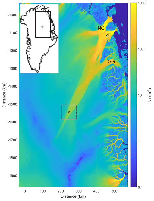
Figure 1 Map of the surface velocity in NE Greenland in meters per year from MEaSUREs Multi-year Greenland Ice Sheet Velocity v1 product, 1995–2015 (Joughin et al., 2016, 2018a), showing the NEGIS ice stream and its three main outlets: Nioghalvfjerdsfjorden Glacier (NG), Zachariae Isstrøm (ZI), and Storstrømmen Glacier (SG). The black box shows the outline of the map in Fig. 2, and the black star indicates the EastGRIP site ($\mathrm{75}{}^{\circ }{\mathrm{38}}^{\prime }$ N, $\mathrm{35}{}^{\circ }{\mathrm{60}}^{\prime }$ W). The inset map shows the location in Greenland.

Here, we present results from a geodetic surface program to characterize surface topography and ice flow of an interior section of NEGIS in an area near its onset in north central Greenland and to assess remote sensing products from this interior area of the Greenland Ice Sheet. The area is located approximately 150 km from the ice stream onset and centered around a reference stake ($\mathrm{75}{}^{\circ }{\mathrm{38}}^{\prime }$ N, $\mathrm{35}{}^{\circ }{\mathrm{58}}^{\prime }$ W) located 300 m from the East Greenland Ice-core Project (EastGRIP) deep-drilling site. We compare our GPS-derived heights and surface velocities with ArcticDEM (Porter et al., 2018), as well as with 165 published and experimental remote sensing velocity products from the NASA MEaSUREs program; the ESA Climate Change Initiative; the PROMICE project; and three experimental products based on data from the ESA Sentinel-1, DLR TerraSAR-X, and USGS Landsat satellites, in order to validate and assess these products (the complete list and references are given in Sect. 4 below). We use the GPS-derived horizontal surface velocities and strain rates in combination with the remote sensing velocity products to characterize the ice stream flow, shear margins, and structure of NEGIS near its onset.

2 GPS data and methods

2.1 GPS stake network

The surface program includes a repeated in situ survey using the Global Positioning System (GPS) with a strain net consisting of 63 stakes. Observations cover the years 2015–2019. The stake network was established in 2015 with 16 stakes, including a central reference stake ($\mathrm{75}{}^{\circ }{\mathrm{38}}^{\prime }$ N, $\mathrm{35}{}^{\circ }{\mathrm{58}}^{\prime }$ W) located 300 m from the EastGRIP deep-drilling site, and gradually expanded in 2016, 2017, and 2018 to include 63 stakes (Fig. 2). The growing network of stakes was measured by GPS every year from 2015 to 2019 and supplemented with additional temporary stakes that were measured only once. The layout of the stakes was designed to provide (1) transects of flow velocities along and transverse to the flow and (2) longitudinal and transverse strain rates in the center of the fast flow and at both shear margins. To fulfill these requirements, the stake network contains sets of stakes placed in a diamond shape centered around the midpoint of NEGIS and at both shear margins. The stake network extends 35 km along NEGIS and 40 km across NEGIS, thereby covering the entire 25 km width of NEGIS and extending across both shear margins into the slower-moving regions outside the ice stream. The purpose of the additional stakes added in 2018 was to obtain detailed information of strain rates across a topographic surface undulation northwest of NEGIS (a 20–30 km dark–bright pattern perpendicular to NEGIS, Fig. 2a). All stake observations are included in this analysis.

Figure 2 Maps of an 80 km × 80 km area around the EastGRIP site showing the GPS stake network (blue dots or circles), the central reference stake at the EastGRIP site (red dot), and the GPS-derived surface velocities (red or black arrows) on an underlying map: (a) detailed surface elevation map (m) from ArcticDEM (Porter et al., 2018) with a velocity scale bar and (b) MEaSUREs Multi-year Greenland Ice Sheet Velocity v1 product (m a⁻¹; Joughin et al., 2016, 2018a) with velocity contours and flow lines. The central flow line through EastGRIP is marked (black line). Ice flow and surface elevations along the central flow line A–A^′ (black) and the three transverse lines B–B^′ (white) are shown in Figs. 3 and 4, respectively. Figure 8 shows additional maps of the area.

The GPS observations were carried out with a Leica GX1230 GPS receiver with data acquisition lasting a minimum of 1 h and typically 2–4 h. The GPS antenna was mounted on the top of each stake, and the height above the surface was measured manually. The stakes were 3.5 m long aluminum stakes, which were drilled approximately 2 m below the surface and extended when needed due to continuous snow accumulation in the area (approximately 0.3 m of snow equivalent per year; Vallelonga et al., 2014). All stakes established in 2015, 2016, and 2017 were extended during the observational period when the antenna heights decreased below 1 m above the surface. A few stakes were moved and/or replaced due to camp activities.

The GPS observations were postfield processed using the open-source software package ESA/UPC GNSS-Lab Tool (gLAB; Sanz Subirana et al., 2013; Ibáñez et al., 2018). We use the Center for Orbit Determination in Europe (CODE) final orbit and clock product, which includes Earth rotation parameters. We took the antenna phase center offset and variation into account. Receiver clock parameters are modeled, and the atmosphere delay parameters are modeled using the CODE maps for the ionosphere and ESA's Niell mapping function with simple nominal values for the troposphere. We applied solid Earth tidal corrections using the IERS Convention's degree 2 tides displacement model (Sanz Subirana et al., 2013). Ocean tidal correction is not implemented in the gLAB processing tool, and for our interior site the associated error is estimated to be within 1 cm. The coordinates are computed in the IGS14 frame. We use the software in static mode and developed an automated protocol in order to perform a systematic precise point positioning (PPP) processing of the stake observations. The PPP approach can introduce systematic errors if the stake is moving (King, 2004). To optimize our processing protocol and evaluate timing estimates and position uncertainties, we observed the central reference stake at the EastGRIP site (red dot in Fig. 2) over extended periods each season and compared separate 1 h static, 24 h static, and kinematic solutions. We found that the 24 h static solution performed better than the average position of a 24 h kinematic solution. With a maximum observed surface speed of approximately 60 m a⁻¹, the uncertainty related to the static solution is estimated to be <2 cm. We estimate the combined uncertainty in our GPS positions to be within 3 cm. We process the stake observations from each year, including multiple observations of some of the stakes within the annual field seasons.

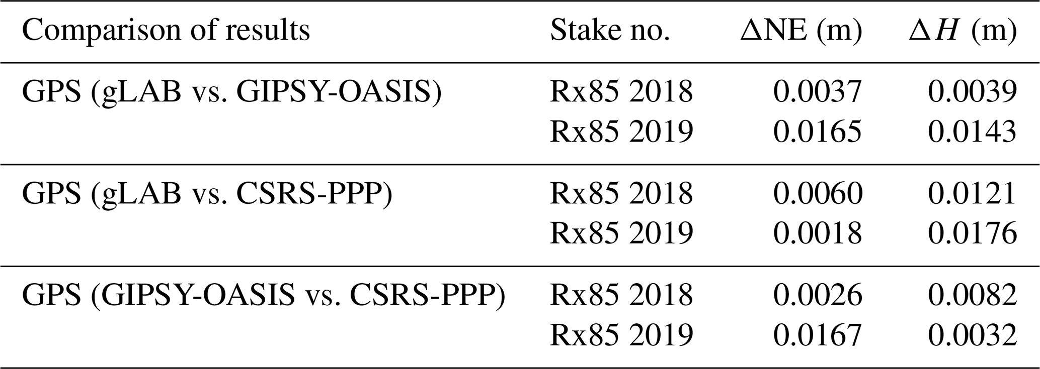
The gLAB processing protocol was assessed by comparing processing results from two 1 h observations with PPP processing results from the GIPSY-OASIS version 6.4 software developed at the Jet Propulsion Laboratory (JPL). We use JPL final orbit products, which include satellite orbits, satellite clock parameters, and Earth orientation parameters. The orbit products take the satellite antenna phase center offsets into account. Receiver clock parameters are modeled, and the atmospheric delay parameters are modeled using the Vienna Mapping Function 1 with VMF1 grid nominal values (http://vmf.geo.tuwien.ac.at/, last access: 13 September 2019; Kouba, 2008; Boehm et al., 2006). Corrections are applied to remove the solid Earth tide and ocean tidal loading. The amplitudes and phases of the main ocean tidal loading terms are calculated using the automatic loading provider (http://www.oso.chalmers.se/, last access: 13 September 2019; Scherneck and Bos, 2002) applied to the FES2014 ocean tide model including correction for center of mass motion of the Earth due to the ocean tides. The site coordinates are computed in the IGS14 frame (Altamimi et al., 2016). All GIPSY-OASIS processing results were within <1.7 cm of the gLAB processing results (Table 1) and within our estimated uncertainty of 3 cm.

Table 1 Assessment of the GPS positions for two stake observations in 2018 and 2019. Top lines: assessment of the processing results, gLAB vs. GIPSY-OASIS. The processing results from the open-source Canadian service CSRS-PPP software v. 1.05 is shown for comparison. ΔNE is the difference in horizontal positions, and ΔH is the difference in vertical positions.

2.2 GPS-derived velocities and surface elevations

To derive the horizontal surface velocity, a linear fit was performed to the observed northing and easting positions, respectively (projected to the National Snow and Ice Data Center – NSIDC – Sea Ice Polar Stereographic North and referenced to the WGS84 horizontal datum – EPSG:3413), assuming a constant displacement rate. A small tilt of the stake can lead to uncertainties in the horizontal velocity. We take this into account by including an unknown horizontal shift in the position of stakes that were vertically extended, and we neglect any other changes in the tilt. For each stake, the shift was determined independently from the other stakes and the linear fit and the shift were determined simultaneously. The estimated shifts are in the range of 0.05 to 0.2 m and often exceed 0.10 m. The surface velocity was calculated by assuming that the flow is along the surface, thereby neglecting vertical movement. We estimate the uncertainty in the derived velocities due to the combined uncertainty in the GPS observations and the method to be on the order of 10⁻² m a⁻¹. As a horizontal reference position of the stakes, we use the estimated horizontal position of the stakes on 1 January 2017, assuming a constant horizontal displacement of each stake over the observational period. We select a common reference for the network in order to consistently derive horizontal strain rates and assess surface elevations, but the reference date is not an accurate timestamp due to the different initial dates of the stakes.

We also estimate a mean GPS-derived surface elevation of the stakes to be used below for the assessment of satellite-based observations. In the interior areas of the Greenland Ice Sheet, climate-driven variations in snow accumulation and firn compaction lead to seasonal and interannual variations in the surface elevation that are not resolved by our annual GPS observations. We estimate the mean GPS-derived surface elevation as the mean of the individual observations at each stake, neglecting trends over the observational period due to changes in snow accumulation, firn processes, or ice dynamical changes.

The resulting horizontal stake velocities are shown in Fig. 2, and the reference positions and horizontal velocities are listed in the Supplement, Table S1. The GPS-derived surface elevations and the magnitudes of the horizontal stake velocities are shown along three transects across NEGIS in Fig. 3 and one transect along NEGIS in Fig. 4. The stake velocities show that the surface speed is relatively constant at approximately 56.6 m a⁻¹ along the centerline of NEGIS and is above 55 m a⁻¹ in the central flow band wider than 10 km. The GPS-derived surface elevations reveal 20 m deep topographic troughs at the shear margins. The direction of the fast flow at the center line is 33.5^∘ from the north.

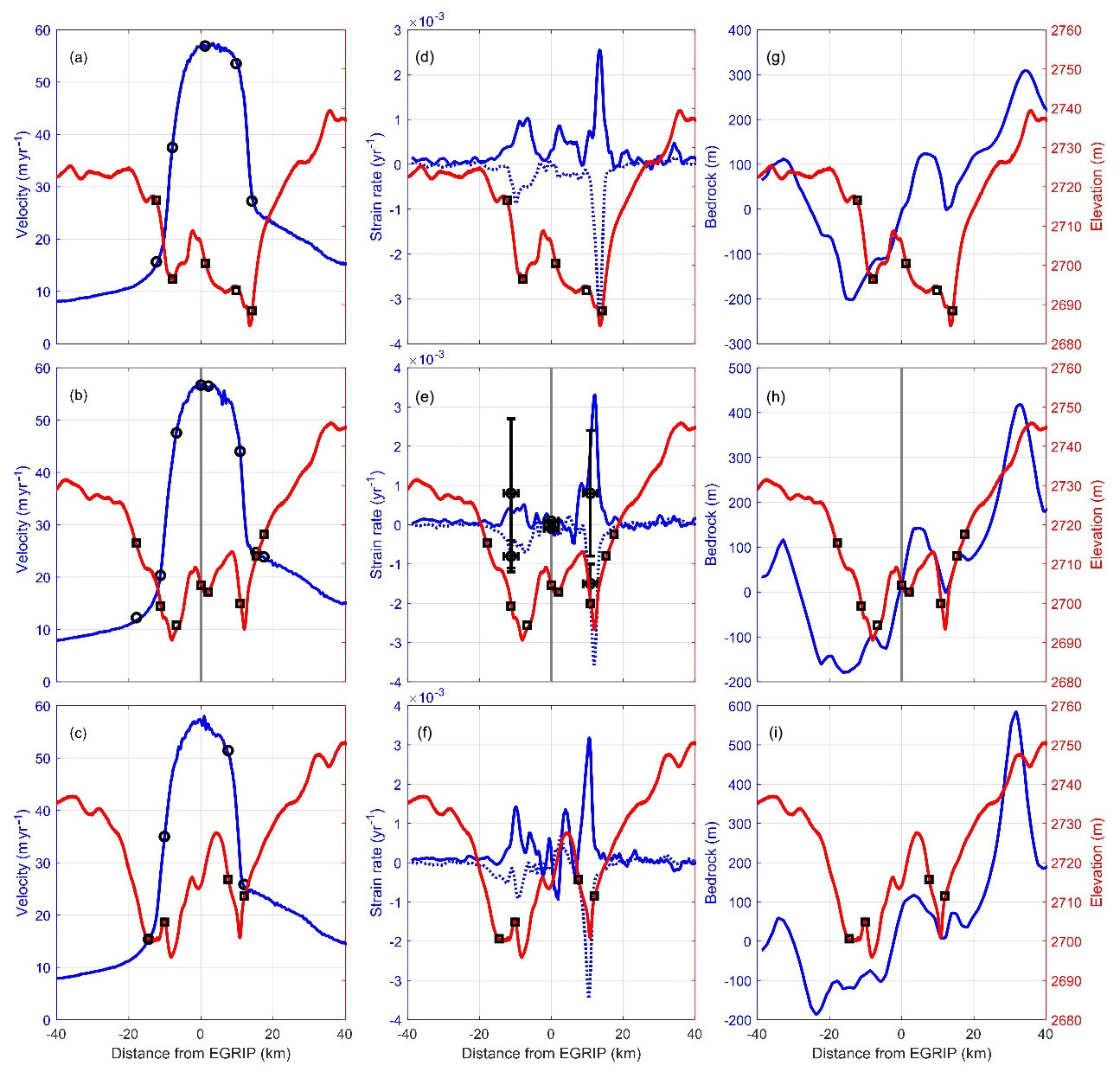
Figure 3 Ice flow and surface elevations of three cross sections of NEGIS separated by 2.5 km: (a, d, g) downstream from the EastGRIP site, (b, e, h) at the EastGRIP site, and (c, f, i) upstream from the EastGRIP site (the cross sections are indicated in Fig. 2b). (a, b, c) Surface velocity (blue) and surface elevation (red). (d, e, f) Surface strain rates relative to the local flow direction, along flow (solid blue) and transverse to flow (dotted blue) with positive for stretching and negative for compression, and surface elevation (red). (g, h, i) Surface elevation (red) and bedrock topography (blue). GPS observations are shown as black circles or squares at three stakes marked in Fig. 5. Surface elevation is from ArcticDEM (Porter et al., 2018); surface velocity and strain rate profiles are derived from the MEaSUREs Multi-year Greenland Ice Sheet Velocity v1 product (Joughin et al., 2016, 2018a); and the bedrock topography is from BedMachine v3 (Morlighem et al., 2017a, b). The vertical gray lines in (b, e, h) indicate the position of the central stake near the EastGRIP site.

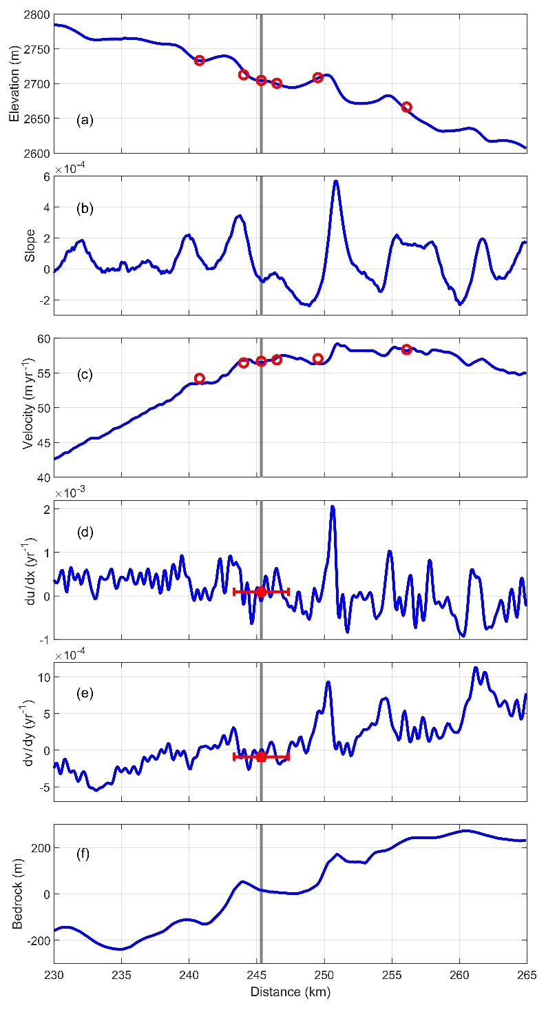
Figure 4 Variations along the central flow line of (a) surface elevation; (b) surface slope; (c) surface velocity; (d) longitudinal strain rate ${\dot{\mathit{ϵ}}}_{x^{\prime }}=\partial u^{\prime }/\partial x^{\prime }$; (e) transverse strain rate ${\dot{\mathit{ϵ}}}_{y^{\prime }}=\partial v^{\prime }/\partial y^{\prime }$, where prime indicates coordinates along and transverse to the flow line; and (f) bedrock topography. The profiles in blue are derived from ArcticDEM (Porter et al., 2018), the MEaSUREs Multi-year Greenland Ice Sheet Velocity v1 product (Joughin et al., 2016, 2018a), and BedMachine v3 (Morlighem et al., 2017a, b). GPS-derived surface elevations, velocities, and strain rates are shown in red. The vertical gray line indicates the position of the central stake near the EastGRIP site.

2.3 GPS-derived strain rates

After having derived horizontal surface velocities, we calculate horizontal strain rates, which are essential in understanding the ice flow pattern and internal stratigraphy of the ice stream and its surroundings. We calculate the horizontal principal strain rates in 32 different triangular sections within the GPS strain net. Each triangle is defined by a combination of three GPS stakes and assumes a linear velocity field within the triangle, i.e., constant strain rates within the triangles (Fig. 5). The principal strain rates are generally on the order of 10⁻⁴ a⁻¹ in a wider-than-10 km central flow band along NEGIS, as well as in the slow-moving areas outside NEGIS. In the two shear margins, horizontal principal strain rates increase by an order of magnitude and reach a maximum in the northern shear margin of $\mathrm{3.8}\times {\mathrm{10}}^{-\mathrm{3}}$ a⁻¹ (horizontal extension) and $-\mathrm{3.6}\times {\mathrm{10}}^{-\mathrm{3}}$ a⁻¹ (horizontal compression) and in the southern shear margin of $\mathrm{3.6}\times {\mathrm{10}}^{-\mathrm{3}}$ a⁻¹ (extension) and $-\mathrm{4.3}\times {\mathrm{10}}^{-\mathrm{3}}$ a⁻¹ (compression). In both shear margins, the principal strain rates are oriented at an angle of approximately ±35^∘ relative to the direction of the flow, due to a combination of longitudinal extension, transverse compression, and a high shear strain rate along the shear margins. The principal strain rates are slightly higher in the triangles north of the central flow line of NEGIS than in those south of the central flow line, probably because the northern shear margin is wider than the southern shear margin and not captured as precisely by the GPS strain net as the southern shear margin. We estimate the uncertainty in the strain rates averaged over the triangles (>2 km) to be on the order of 10⁻⁵ a⁻¹.

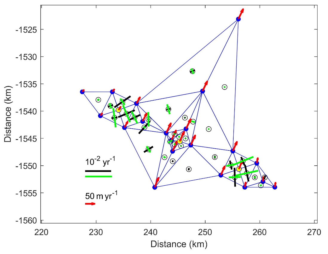
Figure 5 Horizontal principal strain rates for 32 different triangular sections within the GPS array. The principal strain rates are plotted at the centroids of each triangle (black circles) with black lines indicating positive strain rates (extension) and green lines indicating negative strain rates (compression). The GPS-derived surface velocities (red arrows) are plotted at the stakes (blue dots). At three GPS stakes (yellow dots), strain rates along the direction of the flow are calculated.

Along a transect across NEGIS, we calculate the horizontal strain rate tensor along the direction of the flow at three stakes. The three stakes are located in the northern shear margin, in the center (EastGRIP site), and in the southern shear margin, respectively (Fig. 5). The strain rates along the direction of the flow are calculated as the mean of the rotated strain rate tensors in the four adjacent triangles, and they are ±2 km horizontal averages, corresponding to the dimensions of the adjacent triangles. The normal strain rate components along the direction of the flow at these three stakes are plotted in Fig. 3b. At the central flow line at the EastGRIP site, the normal strain rates are $(\mathrm{0.9}\pm \mathrm{0.2})\times {\mathrm{10}}^{-\mathrm{4}}$ a⁻¹ in the longitudinal (along-flow) direction and $(-\mathrm{0.9}\pm \mathrm{0.5})\times {\mathrm{10}}^{-\mathrm{4}}$ a⁻¹ in the transverse direction. The ±2 km average longitudinal and transverse strain rates relative to the local flow direction in the northern shear margin are $(\mathrm{0.8}\pm \mathrm{1.9})\times {\mathrm{10}}^{-\mathrm{3}}$ a⁻¹ and $(-\mathrm{0.8}\pm \mathrm{0.4})\times {\mathrm{10}}^{-\mathrm{3}}$ a⁻¹, respectively. The horizontal shear strain rate is $(-\mathrm{2.1}\pm \mathrm{0.9})\times {\mathrm{10}}^{-\mathrm{3}}$ a⁻¹. The ±2 km average longitudinal and transverse strain rates relative to the local flow direction in the southern shear margin are $(\mathrm{0.8}\pm \mathrm{1.6})\times {\mathrm{10}}^{-\mathrm{3}}$ a⁻¹ and $(-\mathrm{1.3}\pm \mathrm{0.5})\times {\mathrm{10}}^{-\mathrm{3}}$ a⁻¹, respectively, and the horizontal shear strain rate is $(\mathrm{2.6}\pm \mathrm{0.8})\times {\mathrm{10}}^{-\mathrm{3}}$ a⁻¹. The resolution of the GPS strain net is limited by the position of the stakes and may not capture the peak strain rates at the shear margins, but the sharp transition in the southern shear margin stands out in the relative velocity pattern in the Supplement, Fig. S1, and in the strain rates along the transect across NEGIS (Fig. 3b).

3 Data products from satellites

3.1 Satellite-derived digital elevation model

The GPS-derived surface elevations are used to validate the accuracy of ArcticDEM release 7. ArcticDEM is a digital elevation model (DEM) based on stereo auto-correlation techniques on optical imagery from WorldView satellites (Porter et al., 2018). The resolution of ArcticDEM is 2 m with a bias of less than 5 m (Noh and Howat, 2015). The timestamp of ArcticDEM in the EastGRIP area is 2017 (estimated), thus overlapped by the GPS observation period, and the vertical accuracy has not been verified (Porter et al., 2018).

3.2 Satellite-derived surface velocity products

The GPS-derived surface velocities are used to validate and assess the accuracy of several available ice velocity products derived from satellite data from the interior of the Greenland Ice Sheet. The ice velocity can be derived from space using data from synthetic aperture radar (SAR) or optical sensors. Optical feature tracking can provide velocities in very high resolution from coherent pairs of visual images. In the interior of the Greenland Ice Sheet, the surface is mostly featureless and SAR processing methods between pairs of SAR images are useful for deriving surface velocities, based either on speckle tracking or on phase displacements from interferometric synthetic aperture radar (InSAR).

We include several experimental ice velocity products in our assessment, as well as several 1-year and multiyear products constructed from various remote sensing sources and methods. For each type of velocity product, we have also calculated a long-term average of all the velocity maps and included this in our assessment. In total, we include 165 velocity products from the following sources:

1. NASA MEaSUREs Multi-year Greenland Ice Sheet Velocity map v1, 1995–2015 (MEaSUREs Multi-year v1; Joughin et al., 2018a). This map was derived from InSAR, SAR, and Landsat 8 optical imagery data using a combination of speckle-tracking, InSAR, and optical feature-tracking methods, supplemented with balance velocities near the ice divides where the flow speeds are <5 m a⁻¹. The data are provided with a resolution of 250 m. In the interior of the ice sheet, the estimated errors in this product are up to ∼2 m a⁻¹ and reported to be <1 m a⁻¹ in areas where InSAR is used.

2. NASA MEaSUREs Greenland Ice Sheet winter velocity maps (September–May) from InSAR data v2, 2000–2018 (MEaSUREs InSAR v2; Joughin et al., 2010, 2018b). These maps were derived entirely from data obtained by CSA RADARSAT-1, JAXA ALOS, and DLR TerraSAR-X and TanDEM-X (TSX–TDX) satellites, as well as from ESA's C-band SAR data from Copernicus Sentinel-1A and Sentinel-1B. The maps were produced using an integrated set of SAR, speckle-tracking, and interferometric algorithms (Joughin, 2002). The data are provided with a resolution of 200 m, and the error is estimated to be <10 m a⁻¹.

3. NASA MEaSUREs Greenland Annual and Quarterly Ice Sheet velocity maps from SAR and Landsat v1, 2015–2018 (MEaSUREs SAR&Landsat v1; Joughin et al., 2018b). These maps are derived from SAR data obtained by DLR TerraSAR-X and TanDEM-X (TSX–TDX) and ESA Copernicus Sentinel-1A and Sentinel-1B satellites and from the USGS Landsat 8 optical imagery using a combination of speckle-tracking, InSAR, and optical feature-tracking methods (Joughin et al., 2018b). The resolution of the data is 200 m.

4. ESA Climate Change Initiative (ESA CCI) Greenland Ice Sheet annual velocity maps by ENVEO, 2014–2018 from SAR (ESA Greenland Ice Sheet CCI project team, 2018). These maps are derived from ESA Copernicus Sentinel-1A and Sentinel-1B SAR data using feature-tracking techniques. The resolution is 500 m, and the estimated error is ∼15 m a⁻¹ (Nagler et al., 2015).

5. PROMICE Greenland velocity maps, 2016–2019 from SAR (Solgaard and Kusk, 2019). These products are derived from ESA Copernicus Sentinel-1A and Sentinel-1B SAR data using offset tracking (Strozzi et al., 2002) by employing the operational interferometric postprocessing chain (IPP; Kusk et al., 2018; Dall et al., 2015). Each map is a mosaic consisting of both 12 and 6 d pairs within two Sentinel-1 cycles, and thus the temporal resolution of the product is 24 d. A new map is available every 12 d. The spatial resolution is 500 m, and the estimated error is 10–30 m a⁻¹.

6. DTU Space experimental Sentinel-1A and Sentinel-1B Greenland Ice Sheet velocity product, from InSAR (DTU-Space-S1). This product is derived from SAR data acquired by ESA Copernicus Sentinel-1A and Sentinel-1B satellites in the period from 1 to 18 January 2019 from two ascending and three descending tracks. Eight 6 d pairs and five 12 d pairs were processed using the in-house-developed interferometric postprocessing chain (IPP; Kusk et al., 2018). The spatial resolution is 50 m, and the estimated errors are <1 m a⁻¹ (Andersen et al., 2020).

7. AWI experimental TerraSAR-X (TSX) Greenland velocity product, from InSAR (AWI-TSX). The velocity field was derived from SAR interferometry obtained by DLR TSX by combining data from ascending and descending satellite orbits following well-established methods (e.g., Joughin et al., 1998). Three interferograms were formed from descending satellite data acquired between 7 September and 1 October 2016 and another three from ascending satellite data acquired between 24 October 2017 and 3 January 2018. All interferograms have a temporal baseline of 11 d with perpendicular baselines varying between 25 and 180 m. Due to the latter a certain topography-induced phase difference is present in the interferograms, which was removed with the help of the global DLR TanDEM-X DEM with a 30 m grid resolution. The topography-corrected interferograms were unwrapped using GAMMA's minimum-cost flow algorithm (Werner et al., 2002) and combined with 3D velocity maps assuming surface-parallel ice flow. In order to set the relative velocity estimates to absolute values, seed points were extracted from the MEaSUREs Multi-year v1 dataset and adjacent velocity fields were patched together using the average value in their overlapping areas. The final product was gridded to a 30 m spatial resolution. The AWI-TSX product has been developed for this study.

8. MEaSUREs experimental Inter-mission Time Series of Land Ice Velocity and Elevation (ITS_LIVE) annual velocity product version Beta V0 (MEaSUREs ITS_LIVE; Gardner et al., 2019). Surface velocities are derived from image pairs of USGS Landsat 4, 5, 7, and 8 optical imagery using the auto-RIFT feature-tracking processing chain described in Gardner et al. (2018). The final product was gridded to a 120 m spatial resolution. The images suffers from x- and y-geolocation errors of 15 m, and to correct for these errors the velocity components are tied to a stable surface, either to zero at rock surfaces in margin areas or to the median reference velocity in slow-moving areas. In interior Greenland, the MEaSUREs Greenland Annual Ice Sheet Velocity Mosaic from SAR and Landsat version 1 velocity product is used as the reference velocity (Joughin et al., 2010). For the assessment here, we derived a multiyear velocity product from 1985 to 2018, averaged from the annual products. In our observed area, the data are mainly derived from Landsat 8, and we therefore also derived an additional 6-year average of the annual product from 2013 to 2018, covered by the Landsat 8 imagery. These two products were included in the assessment.

4 Comparison between GPS and satellite observations

4.1 Comparison between GPS data and a satellite-derived digital elevation model

We compare GPS-derived surface elevations with the surface elevation sampled from ArcticDEM release 7 at the stake positions (WGS84 ellipsoidal heights) and find an agreement within ±1 m, except for one stake with a deviation of >1.5 m (Supplement Figs. S2 and S3). Minor differences between the two datasets could be due to variable snow accumulation through the years, leading to seasonal and interannual variability in surface elevation, which is captured differently by the two datasets due to their different timestamps. The outlier is located in the exceptionally deep and narrow trough in the southern shear margin (Fig. 3a). Local topography effects at these stakes could possibly be due to interpolation or shadow effects in the Arctic DEM (Porter et al., 2018). The difference between the 63 GPS-derived surface elevations and ArcticDEM at the location of the GPS stakes is 0.48 m (mean) and 0.47 m (median) with a standard deviation of 0.53 m, confirming the low uncertainty in ArcticDEM (Noh and Howat, 2015; Porter et al., 2018).

4.2 Comparison between GPS data and surface velocity products derived from satellite data

The assessment consists of an intercomparison between the GPS-derived velocities of the stakes from the period 2015–2019 and the interpolated surface velocity at the location of the stakes from the satellite-derived velocity products. For each velocity product, we determine the accuracy (the bias) and precision (the standard deviation, i.e., the root mean square difference – RMS – after removing the bias) between the GPS-derived velocities and the satellite-derived velocities at the location of the stakes. In addition to the direct intercomparison between the GPS-derived velocities and the satellite-derived velocities, we also investigate the variability in the satellite-derived velocity products. In order to do so, we perform a spatial smoothing of the satellite-derived velocity product with a running-mean filter with a smoothing length, and we then vary the smoothing length in order to determine the optimum smoothing length (σ) that minimizes the standard deviation (RMS) between the GPS observations and the velocity product. The results of the intercomparison for the top 10 products (sorted according to the standard deviation) are listed in Table 2 (with a complete overview of the results from all products in the Supplement, Table S2), and they are illustrated in Fig. 6.

Table 2 The assessment results for the 10 velocity products with the smallest standard deviation (RMS). The products are sorted with increasing RMS. Notice that the AWI-TSX, the DTU-Space-S1, and the MEaSUREs ITS_LIVE products are also among the 10 products with the smallest bias. The velocity bias is determined for both the x- and y-direction (see Supplement, Table S2). The bias listed here is the length of the velocity bias vector, i.e., the average rate of change in distance between poles moving with the satellite-based velocity field compared to poles moving with the GPS velocities. The complete list of assessment results can be found in the Supplement, Table S2. Dates are given in the format year-month-day.

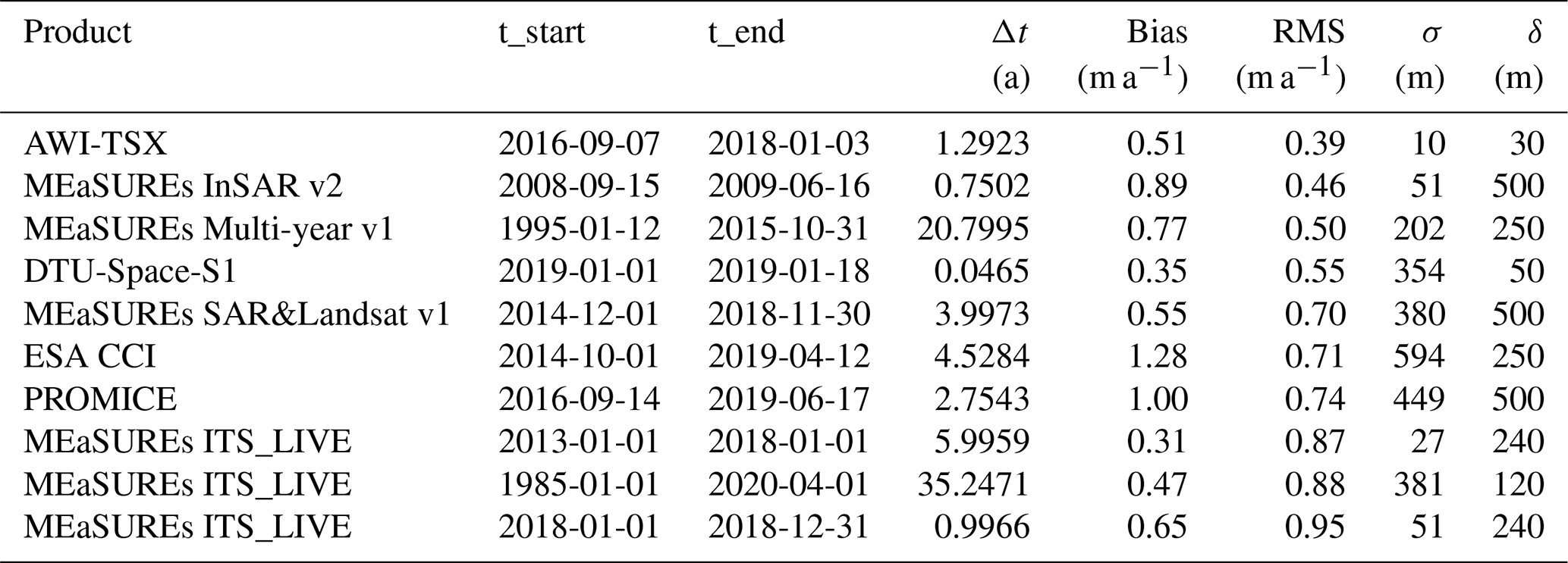
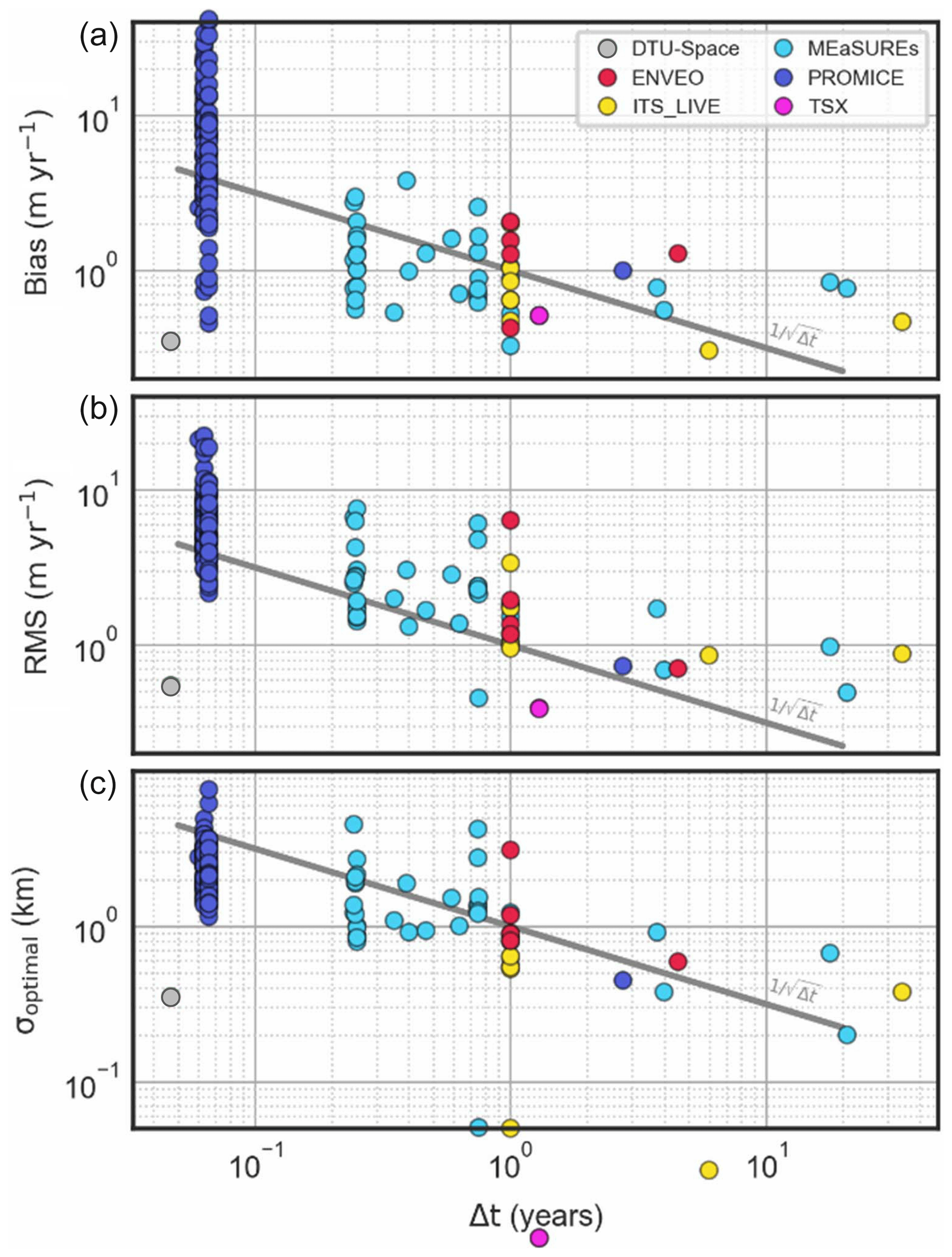
Figure 6 Results of the assessment of a list of 165 satellite-derived surface velocity products: (a) the mean bias in the velocity product compared to the GPS-derived velocities at the location of the GPS poles, (b) the standard deviation of the velocity products relative to GPS-derived velocities (RMS), and (c) the optimal smoothing length of the velocity product that minimizes the standard deviation (σ). All results are shown as a function of Δt, the time span of the velocity product. Notice that some products have been averaged over time to provide results with longer temporal coverage. The gray lines suggest a linear dependency of the bias, RMS, and σ on the inverse of the square of the temporal coverage Δt.

It is important to note that the different timestamps and temporal coverage Δt of the observations are not taken into account in the intercomparison. In satellite-derived velocity products with longer temporal coverage, possible temporal variability and/or noise are smoothed, and there is a clear relationship between increasing temporal coverage and decreasing bias, standard deviation, and optimum smoothing length. Similarly, spatial smoothing can remove noise. The improvement of the products with the temporal coverage Δt is significant, with the bias decreasing approximately linearly with $\mathrm{1}/\sqrt{\mathrm{\Delta }t}$, as illustrated in Fig. 6. Some long-term products were calculated as averages of short-term products, i.e., based on more observations, which would also help reduce the temporal variability in and noise of these products compared to short-term products. The bias in all the 165 products is in the range of ∼0.3–40 m a⁻¹, with a standard deviation in the range of ∼0.4–22 m a⁻¹. The velocity products already include some smoothing as part of their production, but additional smoothing both temporally and spatially, for most products, reduced the standard deviation. After applying optimum spatial smoothing, the standard deviation is reduced to a range of ∼0.4–10 m a⁻¹. The optimum smoothing length σ is typically on the order of 500–3000 m.

As part of the assessment, we use the whole set of satellite-derived surface velocity products to trace flow lines along NEGIS. We use a starting point at the central reference stake near the EastGRIP site, which is located in the center of our observed area in a relatively narrow section of the NEGIS ice stream. We trace the flow lines upstream into the slower-moving areas where flow converges into NEGIS and downstream into faster flow where the ice stream widens (Fig. 7). The flow lines are gradually displaced depending on their bias and fluctuate depending on their standard deviation.

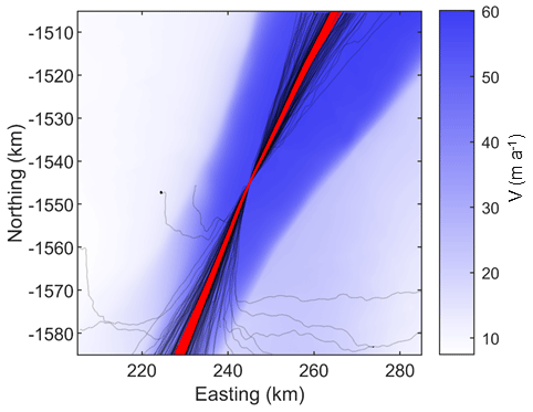
Figure 7 Flow lines through the EastGRIP site (center of plot) calculated from the satellite-derived velocity products. The line thickness depends on the bias in the product, with thick lines having a small bias and vice versa. The top four products with smallest bias are marked with red.

5 Discussion

5.1 Assessment of surface velocity products derived from satellite data

In the interior regions of the Greenland Ice Sheet, validation of satellite-derived ice velocity and surface elevation products is generally limited due to lack of in situ data. Our GPS stake network provides a unique dataset for validation in the interior accumulation area of the ice stream, and it represents a range of velocities and velocity gradients over 1 order of magnitude in the NEGIS ice stream, the shear margins, and the surrounding slow-moving areas. However, the assessment is restricted due to the limited spatial extent of the GPS data, and our conclusions may not apply to margin areas with very fast flow, seasonal variability, or high surface slopes.

In our comparison, the DTU-Space-S1 experimental product stands out among all the investigated products with its short temporal coverage (∼10–20 d); low bias of 0.35 m a⁻¹; and the low standard deviation of 0.55 m a⁻¹, which can be reduced to 0.53 m a⁻¹ after optimum smoothing of 354 m. The AWI-TSX experimental product stands out because of its minimum standard deviation of 0.39 m a⁻¹ of all the investigated products and its high spatial resolution, which results in a very low optimum smoothing length of 10 m, i.e., no further smoothing is needed to reduce the noise, and the bias in the AWI-TSX product is 0.51 m a⁻¹, also among the lowest of the investigated products. Both these products are based entirely on InSAR processing methods.

The widely used MEaSUREs multiyear velocity product, the MEaSUREs Multi-year v1 product (Joughin et al., 2018a), has a bias of 0.77 m a⁻¹ and a standard deviation of 0.50 m a⁻¹. Since this product is already a 20-year average, the optimum smoothing length is only 200 m and only slightly reduces the standard deviation to 0.48 m a⁻¹. It is notable that the bias in this product is similar to several other MEaSUREs products with shorter temporal coverage, while the standard deviation of this product is smaller than the other MEaSUREs products. If the interior of the ice sheet changes slowly over time, the differences between the temporal stamp of the GPS observations and of the multiyear velocity product covering 1995–2015 may become important. However, the MEaSUREs winter velocity map from 2008 to 2009, the MEaSUREs InSAR v2 product, performed very similarly to the MEaSUREs Multi-year v1 product, with a bias of 0.89 m a⁻¹, standard deviation of 0.46 m a⁻¹, and an optimum smoothing length of 51 m. The winter velocity product from 2008 to 2009 is based on InSAR and stands out with its low standard deviation and a relatively short temporal coverage of 9 months. The similar agreement between these products and the GPS-derived velocities suggests that the velocity in the interior part of NEGIS has not changed significantly in the last decade.

The five products with a minimum bias are the MEaSUREs ITS_LIVE 6-year average product with a bias of 0.31 m a⁻¹, the MEaSUREs combined SAR&Landsat v1 1-year product for 2015 with a bias of 0.33 m a⁻¹, the DTU-Space-S1 18 d product from 2019 with a bias of 0.35 m a⁻¹, the ESA CCI annual velocity product from 2015 to 2016 with a bias of 0.43 m a⁻¹, and the 24 d PROMICE product from February 2018 with a bias of 0.46 m a⁻¹. Of these, the DTU-Space-S1 product stands out as mentioned above. MEaSUREs ITS_LIVE product stands out with its long temporal coverage, low standard deviation, and very low optimal smoothing length and because it is the only product in our study entirely based on optical feature tracking. The four other products with a minimum bias have a timestamp that overlaps with the first 1 to 2 years of the GPS observation period, but their standard deviations are much higher due to the SAR speckle-tracking processing techniques. The MEaSUREs combined SAR&Landsat v1 product has a standard deviation of 1.85 m a⁻¹, which reduces to 1.65 m a⁻¹ after optimum smoothing over 1224 m. The ESA CCI product performs very similarly with a standard deviation of 1.94 m a⁻¹, which reduces to 1.11 m a⁻¹ after an optimum smoothing length over 1185 m. The PROMICE product with its very high temporal resolution of 24 d has a standard deviation of 5.39 m a⁻¹, which reduces to 2.6 m a⁻¹ after an optimum smoothing length over 2264 m.

Among the top five products with the lowest standard deviation, three are entirely based on InSAR (DTU-Space-S1, 2019; AWI-TSX, 2016–2017; MEaSUREs InSAR v2, 2008–2009) and two are combined products averaged over a multiyear period (MEaSUREs Multi-year product v1, 1995–2015; MEaSUREs Multi-year SAR&Landsat v1, 2014–2018). Overall, the assessments show that for interior velocity estimates, the InSAR-based products stand out with higher resolution in time and space and with lower errors. SAR speckle-tracking products (ESA CCI, PROMICE, and MEaSUREs) can obtain comparable accuracy and low standard deviation if they are averaged over time (multiyear averages) and smoothed spatially. The optical product (MEaSUREs ITS_LIVE) can obtain a comparably high accuracy when averaged over long time intervals (several years), but the standard deviation is slightly higher than the radar-based products. Mouginot et al. (2017) also derived optical ice velocities from Landsat 8 and concluded similarly that the quality of the products derived from optical satellite sensors is comparable to data obtained with SAR speckle tracking.

5.2 Inferred flow lines from satellite-derived products

Knowing the accurate flow lines of an ice sheet is useful for many applications, such as defining the outlines of drainage basins or identifying the source area for ice flowing through a specific survey site. For studies related to the internal stratigraphy and ice properties, e.g., in ice cores or radar profiles, it is essential to know the upstream flow path in order to infer the deformation history of the internal layers. However, minor uncertainties and bias in satellite-derived velocity products can severely affect flow lines traced along the velocity field, as these uncertainties can displace the flow line and propagate along the flow line (Fig. 7). The flow lines for the products with minimum bias are marked (Fig. 7), showing that flow lines can only be reliably traced if the bias is small. These products have a low bias of 0.31 to 0.43 m a⁻¹ or approximately 1 % of the surface speed. This is particularly critical when the flow is strongly convergent or divergent. We notice that the back trajectories diverge more than the forward trajectories, and we attribute this to the higher uncertainty in the upstream lower velocities compared to downstream. As a result, it may be better to use surface slopes instead of surface velocity products to trace flow trajectories in slow-moving areas.

5.3 Estimated errors in satellite-derived strain rates

Strain rates are derived from the satellite-derived products as derivatives of the velocity fields and have therefore higher errors. Our assessment provides an estimate of the strain rate error depending on the resolution from the standard deviation of the velocity product. For velocity products with a standard deviation on the order of 0.5 m a⁻¹, the strain rate uncertainty is on the order of 10⁻³ a⁻¹ on a 500 m grid, but it could be improved by smoothing the velocity product using the optimum smoothing length from the assessment. We compare the GPS-derived strain rates with strain rates from the MEaSUREs Multi-year Velocity v1 product in transects across NEGIS (Fig. 3) and along NEGIS (Fig. 4). We calculate the satellite-derived strain rate tensor directly from the gridded 250 m resolution velocity product without further smoothing according to the optimum smoothing length (included in Table 2) and rotate according to the local flow direction in order to determine the strain rates along the flow. While the GPS-derived strain rates are limited in resolution and do not exactly capture the maximum strain rate at the southern shear margin, they do capture the enhanced strain rates in the shear margins. The fluctuations in the satellite-derived strain rates are less than 10⁻³ a⁻¹, thus confirming our estimated uncertainty above. The satellite-derived strain rates capture the high-resolution strain rate peaks of approximately 3–$\mathrm{4}\times {\mathrm{10}}^{-\mathrm{3}}$ a⁻¹ in the shear margins (Fig. 3) and approximately $\mathrm{2}\times {\mathrm{10}}^{-\mathrm{4}}$ a⁻¹ along NEGIS (Fig. 4).

5.4 Structure and flow of NEGIS

The assessment of satellite-derived velocity and height products inform us of the accuracy and limitations of the satellite-derived products in the interior regions of the Greenland Ice Sheet. In our study area the best products have a bias and precision of less than approximately 0.5 m a⁻¹, i.e., about 5 % of the smallest observed GPS-derived velocities of around 10 m a⁻¹ in the slow-moving areas north of NEGIS. Knowing the limitations of the satellite-derived products, we are now able to combine the GPS-derived velocities and strain rates with satellite-derived data to characterize spatial patterns in surface structure and ice flow in the interior part of the NEGIS ice stream. We discuss here the observed patterns.

The flow and surface topography across the NEGIS ice stream reveal a distinct 25 km wide fast-flowing ice stream near the EastGRIP site, which is sharply marked at both sides in speed, strain rates, and surface geometry (Fig. 3). The cross sections show a central 10 km wide section with an almost uniform speed of 55 m a⁻¹ and well-defined shear margins at both sides with a width of about 5 km separating the ice stream from the surrounding slow-moving ice (Fig. 3). The velocities are above 20 m a⁻¹ on the southern side where a broad flow field is merging with NEGIS and approximately 10 m a⁻¹ on the northern side (Figs. 2 and 3). The strain rates are at a level of approximately 10⁻⁴ a⁻¹ within the ice stream and in the surrounding slow-moving areas outside the ice stream. In the shear margins, they increase by an order of magnitude to a maximum value of approximately 10⁻³ a⁻¹. The remarkably uniform velocities and low strain rates in the fast-flowing central band of NEGIS with narrow shear zones at the margins with enhanced strain rates are characteristic of ice stream flow (e.g., Minchew et al., 2018). In our study area in NEGIS, Holschuh et al. (2019) proposed that thermal softening of ice is present in the shear margins, despite the relatively low strain rates. The surface topography reveals a 30–40 m deep lowering coinciding with the fast flow within NEGIS with well-defined deep troughs marking the shear margins. These deep shear margin troughs form due to a combination of enhanced longitudinal stretching and shear as the ice flow enters the fast-flowing ice stream from both sides at an angle of ∼15^∘, accelerates, and turns and an enhanced firn densification in the shear margins due to the enhanced horizontal deformation (Riverman et al., 2019a).

The location of the shear margins cannot be clearly linked to the bedrock topography in the area (Christianson et al., 2014; Franke et al., 2020). Christianson et al. (2014) proposed that the shear margins of NEGIS are controlled by a self-stabilizing mechanism related to gradients in the subglacial hydropotential due to the surface troughs that restrict widening of the ice stream, and the internal stratigraphy suggests that the shear margins have been relatively stable during the Holocene (Keisling et al., 2014). Detailed maps of bedrock topography in the area reveal subglacial landforms proposed to be related to basal erosion due to the fast flow (Franke et al., 2020) and elongated bedforms aligned with the flow (Franke et al., 2020; Riverman et al., 2019b). These elongated bedforms are seen in the transects across NEGIS as 100–300 m undulations in bedrock topography (Fig. 3), and they appear here to be related to the location of the shear margins. The southern very well-defined shear margin trough is consistently located above a local bedrock low in the three cross-sectional profiles spanning a 5 km distance along NEGIS (Fig. 3). The northern broad shear margin trough is located over a wide bedrock valley, and the shear margin trough narrows from a wide double trough to a single trough in the three cross-sectional profiles over a 5 km distance along NEGIS, as the bedrock valley over the same distance narrows (Fig. 3). Thus, our observations support that these bedforms are related to the shear margins (Franke et al., 2020; Riverman et al., 2019b), but further studies are needed to fully understand the conditions at the shear margins.

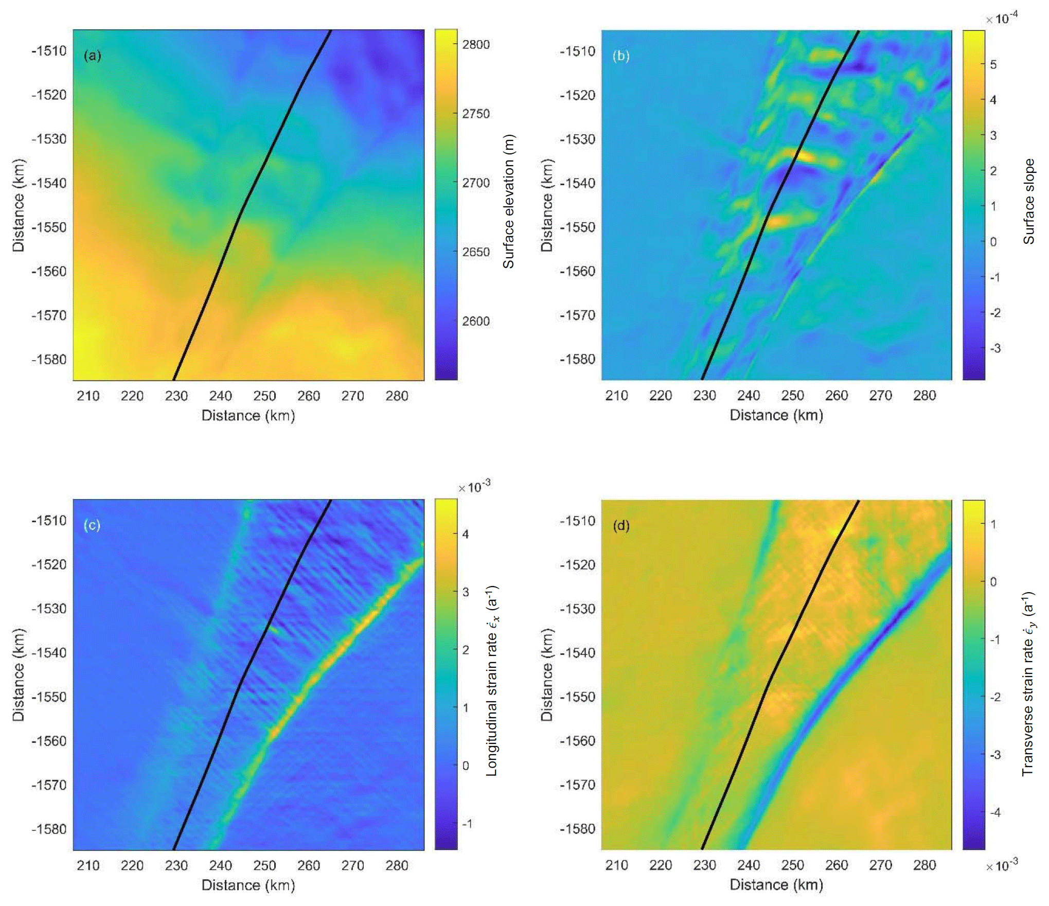
Figure 8 Maps of the 80 km × 80 km section from Fig. 2 with the central flow line marked: (a) surface elevation in meters and (b) surface slope (dimensionless), both derived from ArcticDEM (Porter et al., 2018), and (c) longitudinal strain rate ${\dot{\mathit{ϵ}}}_{x^{\prime }}$ per year along the direction of the flow and (d) transverse strain rate ${\dot{\mathit{ϵ}}}_{y^{\prime }}$ per year along the transverse direction to the flow, both from the MEaSUREs Multi-year Greenland Ice Sheet Velocity v1 product (Joughin et al., 2016, 2018a).

The ArcticDEM surface topography of the NEGIS ice stream shows that an organized spatial pattern of wavy undulations develops perpendicularly to the NEGIS flow in the area around EastGRIP (Fig. 8). The undulations develop within the fast-flowing central flow band of NEGIS in a 25 km section along NEGIS where the surface velocity remains at a level of approximately 55 m a⁻¹. Upstream from this section, the flow accelerates over tens of kilometers with an acceleration of approximately 10 m a⁻¹ over 10 km, i.e. longitudinal strain rates of $\sim {\mathrm{10}}^{-\mathrm{3}}$ a⁻¹. The undulating patterns start forming as ice velocity exceeds a threshold velocity of approximately 55 m a⁻¹ and as the ice flows over a 200–300 m bedrock transition to a bedrock plateau of an approximately 200 m elevation and widens (Franke et al., 2020), suggesting that the undulations are related to the bedrock topography (Fig. 4). The undulations in surface slope are connected to undulations in the longitudinal and transverse surface strain rates and to some degree related to undulations in bedrock topography (Fig. 4). Similar organized undulating patterns in driving stress were previously reported in Antarctic and Greenland ice sheets in fast-flowing areas (Sergienko and Hindmarsh, 2013; Sergienko et al., 2014) and related to patterns in basal stress located in areas with significant sliding. These previous studies attributed the patterns to instabilities related to subglacial water beneath a sliding glacier, and our results support that bedrock topography plays a role in relation to these undulations.

6 Conclusions

We have presented results from a GPS survey in 2015–2019 of a strain net consisting of 63 stakes near the EastGRIP deep-drilling site to map surface topography and flow of an interior section of NEGIS in an area near its onset in interior north Greenland. The GPS-derived surface velocities are >55 m a⁻¹ within an approximately 10 km wide central flow band and drop abruptly at the shear margins to approximately 10 and 25 m a⁻¹ at the northern and southern sides, respectively. The flow enters NEGIS at an angle of approximately 15^∘ from both sides. Strain rates are on the order of 10⁻³ a⁻¹ in the shear margins with enhanced longitudinal stretching, transverse compression, and shearing and are an order of magnitude smaller elsewhere.

We compare our GPS-derived heights and surface velocities with the ArcticDEM height model (Porter et al., 2018), as well as published and experimental remote sensing velocity products in order to validate and assess these products. We include surface velocity products from the MEaSUREs program; the ESA CCI program; the PROMICE program; and experimental data products from MEaSUREs, DTU Space, and AWI. For each product, we calculate the bias, the standard deviation relative to the GPS-derived surface velocities, and the spatial smoothing that minimizes the standard deviation. Our assessments show the following:

• The ArcticDEM height model is accurate at the strain net poles within 0.48 m with a standard deviation of 0.53 m compared to the GPS positions, without considering the different timestamps of the observations. The uncertainty in the GPS positions is on the order of 0.01 m.

• Among the top five surface velocity products with the lowest standard deviation compared to the GPS-derived surface velocities, three are entirely based on InSAR (DTU Space, 2019; AWI-TSX, 2016–2017; MEaSUREs winter velocity by InSAR v2, 2008–2009) and two are combined products averaged over a multiyear period (MEaSUREs Multi-year product, 1995–2015; Measures Multi-year SAR and Landsat, 2014–2018).

• SAR-based surface velocity products from ESA CCI, PROMICE, and MEaSUREs can obtain comparable precision to the GPS-derived surface velocities if they are averaged over longer time periods (years) and smoothed spatially, and they generally obtain a low bias.

• The experimental optical velocity product from MEaSUREs can also obtain a comparable precision to the SAR-based products if it is averaged over long periods (several years), but the bias is slightly higher.

Overall, the assessments show that for interior velocity estimates, the InSAR-based products stand out with higher resolutions in time and space and low errors. For all products, longer observation time improves the products in these interior areas where surface velocity has not changed significantly over the last decade.

This study characterizes the accuracy of the satellite-derived velocities and thereby allows us to evaluate the use of these products for investigations of flow patterns in the interior regions of the Greenland Ice Sheet. We show that satellite-derived strain rates can capture high-resolution spatial signals at the shear margins and within the fast-flowing part of NEGIS, despite the high uncertainty on the order of 10⁻³ a⁻¹. We show further that the strain rate peaks along NEGIS are part of a regular undulating pattern forming in surface slope and strain rates when the surface velocity exceeds approximately 55 m a⁻¹, and we argue that the formation of these undulations appears to be related to bedrock topography.

We derived flow lines from the satellite-derived velocity products and showed that even a minor bias in these products can severely affect the path of the flow lines, in particular in slow-moving areas. We conclude that reliable flow lines can only be derived from satellite-derived velocities with a low bias compared to the surface speed and that surface slopes may produce more realistic flow lines than satellite-derived velocities in slow-moving areas.

The study demonstrates that it is important to know the limitations of the satellite-derived products. We conclude that available satellite-derived products are sufficiently accurate to allow a detailed analysis of the ice flow in the interior part of NEGIS, which can contribute to understanding the flow near its onset in interior north Greenland and ultimately to improving projections of its future response to mass loss at the margins.