the Creative Commons Attribution 4.0 License.
the Creative Commons Attribution 4.0 License.
 | 27 Aug 2020
Quantifying spatiotemporal variability of glacier algal blooms and the impact on surface albedo in southwestern Greenland
Marco Tedesco
Patrick Alexander
Min Xu
Xavier Fettweis
Albedo reduction due to light-absorbing impurities can substantially enhance ice sheet surface melt by increasing surface absorption of solar energy. Glacier algae have been suggested to play a critical role in darkening the ablation zone in southwestern Greenland. It was very recently found that the Sentinel-3 Ocean and Land Colour Instrument (OLCI) band ratio R709 nm∕R673 nm can characterize the spatial patterns of glacier algal blooms. However, Sentinel-3 was launched in 2016, and current data are only available over three melting seasons (2016–2019). Here, we demonstrate the capability of the MEdium Resolution Imaging Spectrometer (MERIS) for mapping glacier algae from space and extend the quantification of glacier algal blooms over southwestern Greenland back to the period 2004–2011. Several band ratio indices (MERIS chlorophyll a indices and the impurity index) were computed and compared with each other. The results indicate that the MERIS two-band ratio index (2BDA) R709 nm∕R665 nm is very effective in capturing the spatial distribution and temporal dynamics of glacier algal growth on bare ice in July and August. We analyzed the interannual (2004–2011) and summer (July–August) trends of algal distribution and found significant seasonal and interannual increases in glacier algae close to the Jakobshavn Isbrae Glacier and along the middle dark zone between the altitudes of 1200 and 1400 m. Using broadband albedo data from the Moderate Resolution Imaging Spectroradiometer (MODIS), we quantified the impact of glacier algal growth on bare ice albedo, finding a significant correlation between algal development and albedo reduction over algae-abundant areas. Our analysis indicates the strong potential for the satellite algal index to be used to reduce bare ice albedo biases in regional climate model simulations.
- Article
(32390 KB) - Full-text XML
- BibTeX
- EndNote


Snow and ice play a critical role in regulating the global energy balance through high surface albedos (Skiles et al., 2018; Warren, 1982). The presence of light-absorbing impurities, including abiotic materials (such as mineral dust and black carbon; e.g., Flanner et al., 2007; Goelles and Bøggild, 2017; Wientjes et al., 2011) and biogenic materials primarily produced by microbial processes (Chandler et al., 2015; Ryan et al., 2018; Stibal et al., 2017; Williamson et al., 2019), can substantially reduce the surface albedo of snow and ice and thus enhance surface melt. Increased meltwater further decreases surface albedo, triggering a positive feedback mechanism between meltwater production and albedo decline (Box et al., 2012; Tedesco et al., 2011, 2016).
Snow algae and glacier algae are among the main microbial communities in supraglacial environments, which are distributed in Greenland, Antarctica, Alaska, Svalbard, the Himalayas, Siberia, the Rocky Mountains, and the European Alps (Anesio et al., 2017). Algal growth on glaciers and ice sheets not only plays an important role in local and regional carbon and nutrient cycles but is also crucial for regulating surface melt processes through the reduction in snow and ice albedo resulting from dark algae pigmentation (Lutz et al., 2014; Remias et al., 2012; Stibal et al., 2017; Yallop et al., 2012). Snow algae (mainly Chlorophyceae) are psychrophiles residing in glacial snow or snowfields and bloom on the snow surface after the onset of melting (Lutz et al., 2016, 2017). The visible color of snow algae varies from green to yellow to orange and red and is determined by the pigments (chlorophylls, xanthophylls, and secondary carotenoids, etc.) produced in different life stages (Anesio et al., 2017). Glacier algae (Zygnematales) are different from snow algae and grow on the bare ice glacier surface when liquid water, nutrients, and photosynthetically active radiation are sufficient (Lutz et al., 2018; Stibal et al., 2017; Yallop et al., 2012). The earliest documentation about glacier algae dates to 1872. During an expedition to Greenland in 1870, Adolf Erik Nordenskiöld and fellow explorers found “a brown polycellular alga” on the ice surface and within cryoconite holes (Nordenskiöld, 1872). Several field studies (Lutz et al., 2018; Stibal et al., 2015, 2017; Uetake et al., 2010; Yallop et al., 2012) have investigated the species composition and cell structures of glacier algal communities. The primary glacier algal species are Ancylonema nordenskiöldii, Mesotaenium berggrenii, and Cylindrocystis brebissonii, which are green microalgae and produce pigments including chlorophyll a, chlorophyll b, beta-carotene, lutein, and violaxanthin. Ancylonema nordenskiöldii and Mesotaenium berggrenii also generate a phenolic purpurogallin pigment (purpurogallin carboxylic acid-6-O-b-D-glucopyranoside), which absorbs ultraviolet and visible radiation (Remias et al., 2012; Yallop et al., 2012). It has been suggested that this purpurogallin pigment accounts for the brownish-grey color of the algae-laden ice (Remias et al., 2012; Yallop et al., 2012).
Recent studies have revealed a significant impact of glacier algal blooms on bare ice albedo in Greenland (Stibal et al., 2017; Tedstone et al., 2020; Williamson et al., 2018). Along the ablation zone over the southwestern Greenland Ice Sheet, a dark ice band appears every summer season (Shimada et al., 2016; Tedstone et al., 2017). It was previously thought that this surface darkening was primarily caused by outcropping of ancient dust (Wientjes and Oerlemans, 2010). Recently, widespread glacier algal blooms were observed in the field, and the dark pigments generated by glacier algae were argued to be a primary control on the presence of the dark band (Ryan et al., 2018; Stibal et al., 2017; Williamson et al., 2018, 2020). Field sampling and spectral measurements indicate that glacier algae have a greater effect on albedo reduction than other non-algal impurities (Stibal et al., 2017). However, current field measurements of glacier algal abundance and surface albedo are limited to very few sites and melting seasons, and it is logistically difficult to use laboratory techniques to measure glacier algae at a regional scale. The impact of glacier algal development on surface albedo over large spatial and temporal scales has not yet been quantified.
Remote sensing provides a synoptic and efficient way to characterize geospatial phenomena across large spatial scales. To date, using remote sensing methods to quantify snow or glacier algae extent or concentration is limited to a few studies (e.g., Cook et al., 2020; Ganey et al., 2017; Huovinen et al., 2018; Painter et al., 2001; Takeuchi et al., 2006; Wang et al., 2018). Painter et al. (2001) estimated the algal abundance of the snow alga Chlamydomonas nivalis over a snow-covered region in the Sierra Nevada of California from Airborne Visible/Infrared Imaging Spectrometer (AVIRIS) hyperspectral imagery based on chlorophyll a absorption features between 630 and 700 nm. Despite the high capability of airborne hyperspectral imaging data for detecting chlorophylls, the availability of hyperspectral imaging data is constrained over space and time. Several studies (e.g., Takeuchi et al., 2006; Ganey et al., 2017; Huovinen et al., 2018) mapped red snow algae based on carotenoid absorption features using satellite red and green bands.
Mapping glacier algae using remote sensing is complicated by a number of factors, including the complex pigmentation of glacier algae, insufficient spectral and spatial resolution of satellite data, and the impact of dusts and underlying ice optics that are not yet well understood. The use of carotenoid features is not applicable to glacier algae, as they do not, to our knowledge, generate secondary carotenoids like snow algae (Painter et al., 2001; Takeuchi et al., 2006). The brownish-grey color of glacier algae is attributed to the purpurogallin pigments, but the characteristic absorption peaks of purpurogallin pigments are concentrated in the ultraviolet spectrum at 278, 304, and 389 nm (Remias et al., 2012), which are not detectable by current satellite sensors. At visible wavelengths, the absorption by purpurogallin pigments is quite uniform, making it difficult to differentiate between glacier algae and other dark impurities from satellite data based on purpurogallin spectral properties.
The spectral signature of chlorophyll a, the primary photosynthetic pigment generated by glacier algae, however, is well-suited for mapping glacier algae using satellite remote sensing techniques. Chlorophyll a is widely used as a biomarker to detect or quantify algal blooms from remote sensing data (e.g., Gitelson, 1992; Painter et al., 2001), and it was recently found that the spectral signatures of chlorophyll a in the red and near-infrared (NIR) region can be utilized for mapping glacier algae (Wang et al., 2018). The red–NIR spectral signature of chlorophyll a, i.e., absorption at 665–681 nm and reflectance around 709 nm, is present in field hyperspectral data collected over ice surfaces covered by glacier algae (Cook et al., 2020; Stibal et al., 2017). The concentration of chlorophyll a is generally used as a proxy for algal biomass or abundance and based on this a number of algorithms have been developed to quantify the biomass contained in algal blooms occurring in aquatic systems (Beck et al., 2016; Blondeau-Patissier et al., 2014; Matthews, 2011; Xu et al., 2019a, b). Using the two-band ratio (R709 nm∕R673 nm) method, Wang et al. (2018) quantified the spatial distribution of glacier algal blooms in southwestern Greenland over the summer seasons in 2016 and 2017 from the Sentinel-3 Ocean and Land Colour Instrument (OLCI) data. Despite the moderate (300 m) spatial resolution, the derived spatial pattern based on the red–NIR chlorophyll a signature matches well with previous field observations (Stibal et al., 2015, 2017; Williamson et al., 2018). As for higher spatial resolution remote sensing data, Cook et al. (2020) applied a random forest method to classify unmanned aerial vehicle (UAV) and the Sentinel-2 Multispectral Instrument (MSI) data for identification of high-algae biomass and low-algae biomass areas. However, these data have limitations in terms of spatial coverage, temporal resolution, and spectral resolution. To establish a long-term time series quantification of glacier algae distribution and study the seasonal process of glacier algal blooms and the impact on albedo change, the use of chlorophyll a-sensitive ocean color satellite sensors is promising.
The Sentinel-3 OLCI is equipped with 21 spectral bands, including 7 narrow chlorophyll a bands. The advanced band configuration of OLCI makes it a valuable sensor for mapping algal blooms not only in water but also on ice (Wang et al., 2018). OLCI was designed based on the opto-mechanical and imaging design of the MEdium Resolution Imaging Spectrometer (MERIS) onboard the European Space Agency (ESA)'s Envisat satellite, operational from March 2002 to April 2012, which collected data in 15 spectral bands between 390 and 1040 nm. MERIS features in particular a 709 nm band where high levels of chlorophyll a produce a characteristic reflectance peak. MERIS data have been broadly used for atmospheric and oceanic studies, with the primary goal of measuring the concentration of chlorophyll a and suspended sediments in oceans, coastal waters, and inland lakes (Gower et al., 2008; Palmer et al., 2015). Similar configurations of the chlorophyll-targeted bands in terms of wavelength and bandwidth between MERIS and OLCI (Fig. 1a) point to the potential of using MERIS data to reconstruct the spatial distribution of glacier algae prior to 2012. In this study, we make use of the capability of MERIS for detecting chlorophyll a to extend the quantification of glacier algae in southwestern Greenland back to the 2004–2011 period, and further quantify the impact of glacier algal blooms on bare ice albedo by combining the time series data of MERIS and MODIS.
2.1 Study area and previous field observations
Our study area is located between 66–71∘ N and 47–51∘ W in southwestern Greenland. This area features high ablation rates and low surface albedos during summertime (Alexander et al., 2014; Fettweis et al., 2011; Moustafa et al., 2015; Stroeve et al., 2013). With the progression of surface melt over time, a dark ice zone forms rapidly and reaches a maximum area from mid-July to mid-August (Tedstone et al., 2017; Wang et al., 2018). The bare ice and dark ice areal extent is highly correlated with meltwater production and surface runoff simulated by the regional climate model Modèle Atmosphérique Régionale (MAR) (Wang et al. 2018). The peak time of surface darkening coincides with the occurrence of glacier algal blooms observed in the field. The ice alga Ancylonema nordenskiöldii and Mesotaenium berggrenii are the dominant species found in southwestern Greenland during July and August (Lutz et al., 2018; Yallop et al., 2012; Williamson et al., 2018). Considering the growth season and surface habitat of glacier algae, we focus our analysis on bare ice in July and August.
There are a limited number of field studies measuring glacier algal abundance and reflectance spectra over the study area (Cook et al., 2020; Stibal et al., 2015, 2017; Williamson et al., 2018), and no field measurements were coincident with the acquisition time of the Envisat MERIS data. Here we utilized the previous field observations in a qualitative way for comparison purposes, and explored the extension of an empirical function derived from Sentinel-3 OLCI data (Wang et al., 2018) to MERIS data for characterizing the temporal variations of algal population with surface albedo change. We utilized field data first presented by Stibal et al. (2015, 2017) to validate patterns of spatial variability in glacier algae distribution and to compare with satellite data to validate the chlorophyll a spectral signal. Stibal et al. (2015) collected shallow surface ice cores and measured algal abundance over 14 sites in Greenland during May–September 2013, of which the sites DS (69∘28.56′ N, 49∘34.838′ W), KAN_M (67∘3.964′ N, 48∘49.356′ W), and KAN_L (67∘5.798′ N, 49∘56.303′ W) are within our study area. KAN_M and KAN_L are located along the Kangerlussuaq transect (K-transect), and DS is located near the Jakobshavn Isbrae Glacier. Stibal et al. (2015) documented the algal abundance averaged over the sampling season (2013 summer) for each site, finding cell counts of 66 ± 31 cells mL−1 (KAN_L), 5688 ± 3147 cells mL−1 (KAN_M), and 10 621 ± 2073 cells mL−1 (DS), respectively. During the 2014 summer season, Stibal et al. (2017) collected both algal abundance and hyperspectral reflectance measurements via an Analytical Spectral Devices (ASD) Field Spectrometer over a site near the automatic weather station S6 (67∘04.779′ N, 49∘24.077′ W) on the K-transect. They collected multiple samples each observation day and published the datasets of glacier algal abundance and reflectance spectra at a 10 nm spectral resolution (Stibal et al., 2017). Here we used the field hyperspectral data to compare with the satellite spectra to validate the chlorophyll a signal.
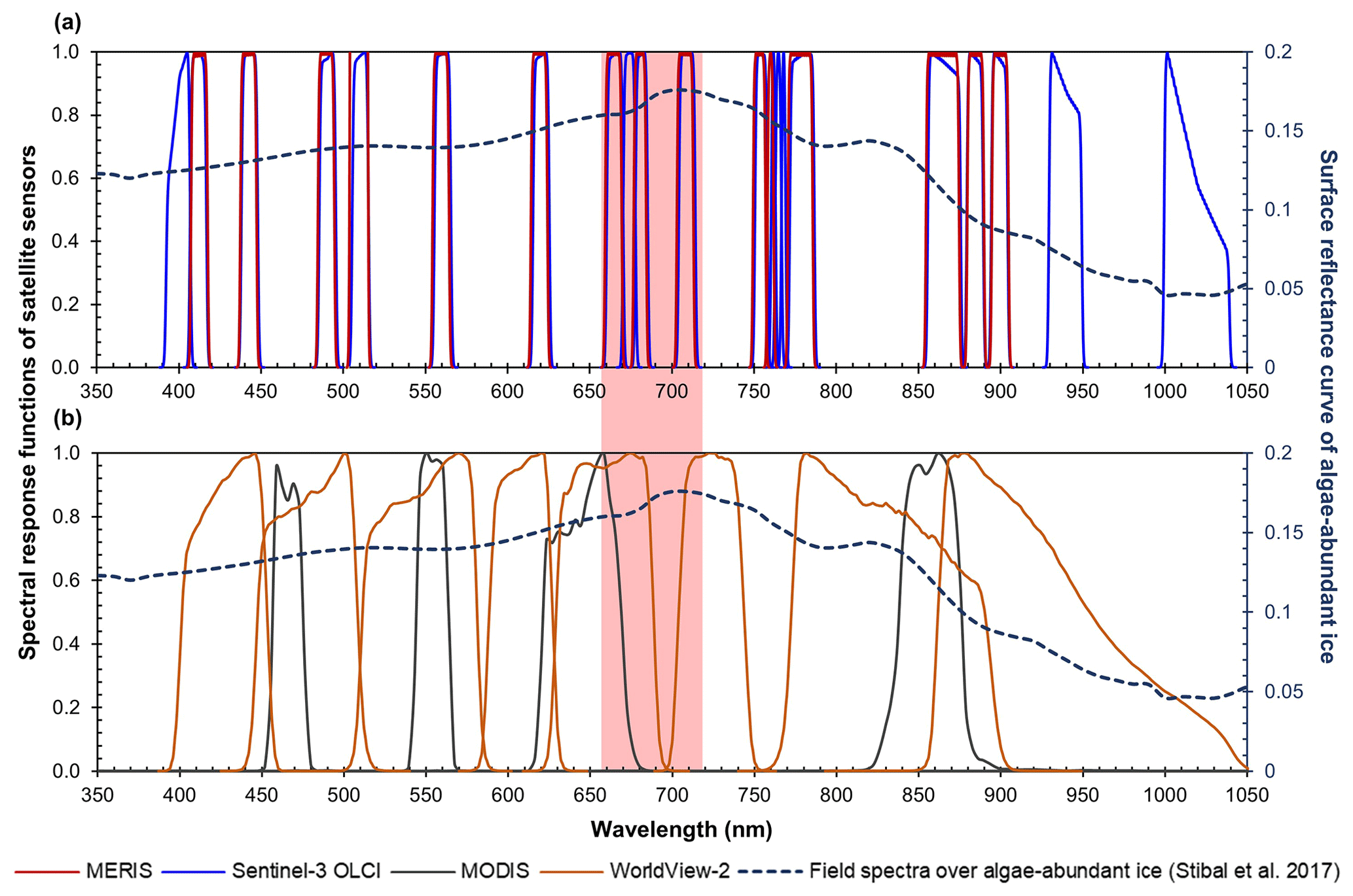
Figure 1Spectral response functions of (a) MERIS (red) and OLCI (blue) and (b) MODIS (black) and WorldView-2 (orange) over the wavelength range of 350–1050 nm. All the MERIS and OLCI bands are within the 350–1050 nm range, where photosynthetic and photoprotective pigments have spectral responses. Four MODIS bands (over land) and eight WorldView-2 bands are within this spectral range but with much coarser spectral resolutions. In both subplots, the dashed line shows hyperspectral ASD field spectrometer data (right vertical axis) collected over algae-abundant ice by Stibal et al. (2017), containing chlorophyll a signal at the red–NIR wavelengths (red-highlighted region). The plotted field spectrum (sample code: Ab.25.06.14.D1) was measured on 25 June 2014 at 67∘04.779′ N, 49∘24.077′ W (near the automatic weather station S6 along the K-transect), with an algal abundance measurement of 121 664 cells mL−1 (Stibal et al., 2017).
2.2 Satellite data
2.2.1 MERIS Level-2 data
We used the full spatial resolution (300 m) MERIS Level-2 data acquired during July and August from 2004 to 2011 (https://earth.esa.int/web/guest/-/meris-full-resolution-full-swath-6015, last access: 1 August 2019). The MERIS Level-2 data were processed from the Level-1b data (top-of-atmosphere radiances in 15 spectral bands shown in Fig. 1a). ESA adopted different processing techniques to generate the Level-2 data over land, water, and clouds. The Level-2 data over land include the normalized surface reflectance in 13 spectral bands, corrected for the atmospheric effects of gaseous absorption and stratospheric aerosols (ESA, 2011b). The full resolution Level-2 data from May 2002 to April 2012 were released at the MERCI file archive (https://merisfrs-merci-ds.eo.esa.int/, last access: 1 August 2019) in February 2015. We identified 146 cloudless MERIS images acquired on 135 d from July to August between 2004 and 2011. Since there were no cloudless images available for the 2002 summer season and only three images for the 2003 summer over the study area, we excluded these 2 years from our analysis. For those images affected by clouds over the study area, we checked the MERIS Level-2 Flag data including the pixel types classified as water, land, and cloud. However, the Flag data fail to correctly capture all the cloud pixels due to limitations of the algorithm in differentiating clouds from other bright surfaces like snow and ice (ESA, 2011a). In this regard, we manually removed the cloud pixels (patches) from each MERIS image.
2.2.2 MODIS data
We used the MODIS/Terra daily surface reflectance product (MOD09GA Version 6) and daily snow cover product (MOD10A1 Version 6). The MOD09GA data include the atmospherically corrected surface reflectance for the 620–670, 841–876, 459–479, 545–565, 1230–1250, 1628–1652, and 2105–2155 nm MODIS bands (Fig. 1b). The MOD10A1 data include broadband albedo estimated based on the MOD09GA product. We used the version 6 data, which are greatly improved in sensor calibration, cloud detection, and aerosol retrieval and correction relative to version 5 (Casey et al., 2017; Lyapustin et al., 2014; Toller et al., 2013). Version 6 data are recommended for assessing temporal variability of surface albedo since they are corrected for sensor degradation issues that impacted earlier versions (Casey et al., 2017). The spatial resolution of the MODIS datasets is 500 m. We resampled the MODIS data to 300 m using a nearest-neighbor resampling method. The cloud masks in the MOD10A1 data were applied to exclude clouds.
2.2.3 WorldView-2 imagery
We also used WorldView-2 imagery to validate the spectral signal of glacier algae captured by MERIS data. The WorldView-2 satellite was launched in October 2009, collecting data in nine spectral bands (panchromatic, coast, blue, green, yellow, red, red edge, NIR, and NIR2; Fig. 1b) at a very high spatial resolution (∼ 2 m for the multispectral bands). WorldView satellites have high geolocation accuracy, owing to their three-axis stabilized platform equipped with high-precision GPS and attitude sensors (Wang et al., 2016). Although the WorldView-2 spectral bands have wide bandwidths, the red (630–690 nm) and red edge (705–745 nm) bands can capture the chlorophyll a signal (Fig. 1b) and have been used for mapping algal species in nearshore marine habitats (Reshitnyk et al., 2014). We obtained WorldView-2 imagery acquired in July and August (2009–2011) from the Polar Geospatial Center (PGC, https://www.pgc.umn.edu/, last access: 1 August 2019). The images were provided as orthorectified top-of-atmospheric radiances in eight multispectral bands. We performed atmospheric corrections to the radiance images and obtained surface reflectance images using the MODerate resolution atmospheric TRANsmission (MODTRAN)-based Fast Line-of-sight Atmospheric Analysis of Hypercubes (FLAASH) (Anderson et al., 2002). The subarctic model and rural aerosol model were used for correction of atmospheric effects caused by water vapor and aerosols (Legleiter et al., 2013).
2.3 Modèle Atmosphérique Régionale (MAR) outputs
The regional climate model Modèle Atmosphérique Régionale (MAR, Fettweis et al., 2017) combines atmospheric modeling (Gallée and Schayes, 1994) with the Soil Ice Snow Vegetation Atmosphere Transfer Scheme (De Ridder and Gallée, 1998) to simulate surface energy balance and mass balance processes over the Greenland and Antarctic ice sheets. In this study, we examined the relationship between the MAR albedo bias (e.g., Alexander et al., 2014; Moustafa et al., 2015) and glacier algal blooms. The snow albedo in MAR is determined by snowpack temperature, temperature gradient, and liquid water content, and the bare ice albedo is scaled based on the accumulated surface water (Zuo and Oerlemans, 1996; Alexander et al., 2014). Since the MAR albedo scheme does not account for impurities, there are significant biases in MAR albedo over the southwestern Greenland ablation zone (Alexander et al., 2014). We used the 7.5 km resolution MAR v3.9 daily outputs, forced by the European Centre for Medium-Range Weather Forecasts Interim Reanalysis (ERA-Interim; Dee et al., 2011).
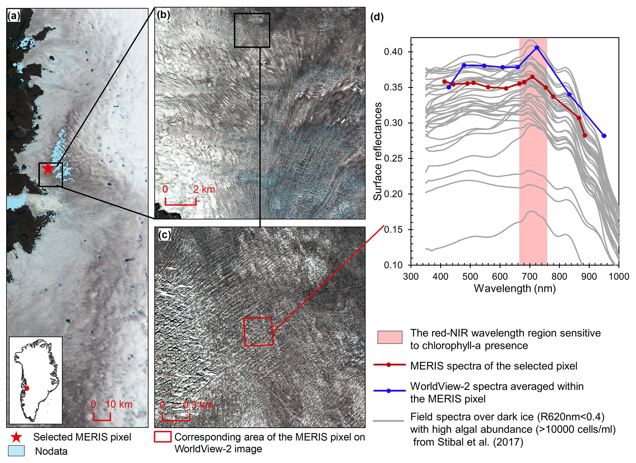
Figure 2Comparison between MERIS, WorldView-2, and field spectra over algae-abundant dark ice. (a) MERIS Level-2 image (true color composite) acquired on 5 July 2010. Pixels with missing data are shown in light blue. (b) WorldView-2 surface reflectance image (© 2010 DigitalGlobe, Inc.) acquired on 9 July 2010 over the square area in (a). (c) Zoomed-in WorldView-2 image, with the area (red square) corresponding to the selected MERIS pixel in (a). (d) Reflectance spectra for MERIS and WorldView-2 (2010) and field hyperspectral measurements collected over the algae-abundant dark ice at S6 by Stibal et al. (2017) in 2014.
3.1 Bare ice mapping
We mapped bare ice cover from each MERIS image using a thresholding method applied to surface reflectance data (e.g., Shimada et al., 2016; Tedstone et al., 2017; Wang et al., 2018). To be consistent with previous studies, we used MODIS-derived bare ice maps as a reference to determine the optimal threshold for the MERIS data. We removed tundra and ocean pixels using the MEaSUREs Greenland Ice Mapping Project classification mask (Howat et al., 2014). We selected 31 MOD09GA images that were coincident with MERIS overpasses and were cloud free over the study area. Following Tedstone et al. (2017), we applied a threshold to the MODIS 841–876 nm reflectance (R841−876 nm), using the criterion R841−876 nm < 0.6 to extract bare ice reference maps from selected MODIS images. For coincident MERIS images, we iteratively applied a threshold value ranging from 0 to 1, increasing by 0.01 at each iteration to the MERIS band 13 (865 nm) and compared the MERIS and MODIS bare ice cover. The optimal threshold was determined based on the F1 score accuracy metric, which is the harmonic average of precision and recall, defined as follows:
where precision is calculated as and recall is calculated as . NTP is the number of true positives (the number of pixels classified as bare ice by both the MODIS and MERIS data), NFP is the number of false positives (the number of pixels that are only classified as bare ice by the MERIS data), and NFN is the number of false negatives (the number of pixels that are only classified as bare ice by the MODIS data). The average F1 score was calculated for each threshold based on those 31 image pairs. The threshold of 0.53 yielded the highest F1 score (0.957). We excluded supraglacial lakes using the modified normalized difference water index (MNDWI, Yang and Smith, 2013), defined as follows:
where Rblue is the reflectance at 442 nm (MERIS band 2) and Rred is the reflectance at 665 nm (MERIS band 7). Pixels with MNDWI greater than 0.14 (Yang and Smith, 2013) were identified as lake pixels and excluded from analysis. Using the same iterative method described above, we also determined an optimal threshold of 0.47 to extract dark ice pixels (pixels with bare ice containing substantial surface impurities) using the 620 nm MERIS band, following Shimada et al. (2016) and Tedstone et al. (2017). This band has been used to delineate dark ice by applying a threshold based on the assumption that visible wavelengths including the red band are mostly affected by light-absorbing impurities rather than surface water and grain size variations (Shimada et al., 2016; Tedstone et al., 2017; Wang et al., 2018).
3.2 Chlorophyll a indices and impurity index
Chlorophyll a is the primary photosynthetic pigment generated by glacier algal cells (Williamson et al., 2018; Yallop et al., 2012). Hyperspectral field measurements (Fig. 2d, Cook et al., 2020; Stibal et al., 2017) and the Sentinel-3 OLCI spectra (Wang et al., 2018) both exhibit the typical spectral signatures of chlorophyll a at the red and NIR wavelengths over algae-abundant ice surfaces, featuring a reflectance peak around 709 nm and absorption features around 665–681 nm. Pure ice has lower reflectance at 709 nm compared to shorter wavelengths (Hall and Martinec, 1985). The magnitude of the reflectance peak at 709 nm relative to 665–681 nm is highly dependent on the chlorophyll a content (Binding et al., 2013; Gitelson, 1992). Figure 2d shows the MERIS spectra over a dark ice pixel, compared with WorldView-2 spectra and field hyperspectral measurements by Stibal et al. (2017). The selected MERIS pixel, located near the Jakobshavn Isbrae Glacier, is close to the site DS, where Stibal et al. (2015) measured a high abundance of glacier algae during the 2013 summer season. The MERIS image (Fig. 2a) was acquired on 5 July 2010, and the WorldView-2 image (Fig. 2b and c) was acquired on 9 July 2010. The field hyperspectral curves shown in Fig. 2d were measured over dark ice (R620 nm < 0.4) with high algal abundance (greater than 10 000 cells mL−1), featuring chlorophyll a signatures in the red–NIR region. Despite the differences in absolute values of surface reflectance, the spectral shapes of the MERIS, WorldView-2 and field spectra match quite well, particularly with regard to the presence of chlorophyll a, validating the ability of MERIS data to capture the glacier algae spectral signal.
Table 1Equations and MERIS bands used for calculation of different ratio indices.

To map glacier algae using the chlorophyll a spectral signature, we calculated several MERIS chlorophyll a indices (Table 1), including the two-band NIR–red index (2BDA), three-band NIR–red index (3BDA), normalized difference chlorophyll index (NDCI), and maximum chlorophyll index (MCI) (Moses et al., 2012; Mishra and Mishra, 2012; Binding et al., 2013). The 2BDA and 3BDA methods have been widely applied to estimate chlorophyll a concentration in aquatic systems using MERIS data (Beck et al., 2016; Moses et al., 2009; Xu et al., 2019a, b) and have proved to be highly accurate for chlorophyll a retrieval in turbid coastal waters characterized by complex optical properties (Moses et al., 2012). The NDCI (Mishra and Mishra, 2012) was defined based on the concept of the normalized difference vegetation index (NDVI). The MCI measures the height of the 709 nm reflectance peak relative to the baseline obtained by interpolating reflectance between 681 and 753 nm (Binding et al., 2013). In addition, we also calculated the impurity index (Dumont et al., 2014) for comparison with the chlorophyll a indices. The impurity index is the ratio between the natural logarithms of the spectral albedos at the green and NIR bands and was constructed to quantify the impurity content over the Greenland Ice Sheet upon the assumption that the visible wavelengths are much more sensitive to impurity content than the NIR wavelengths. Radiative transfer modeling experiments have shown that the impurity index is less affected by snow grain size variations than the presence of impurities (Dumont et al., 2014).
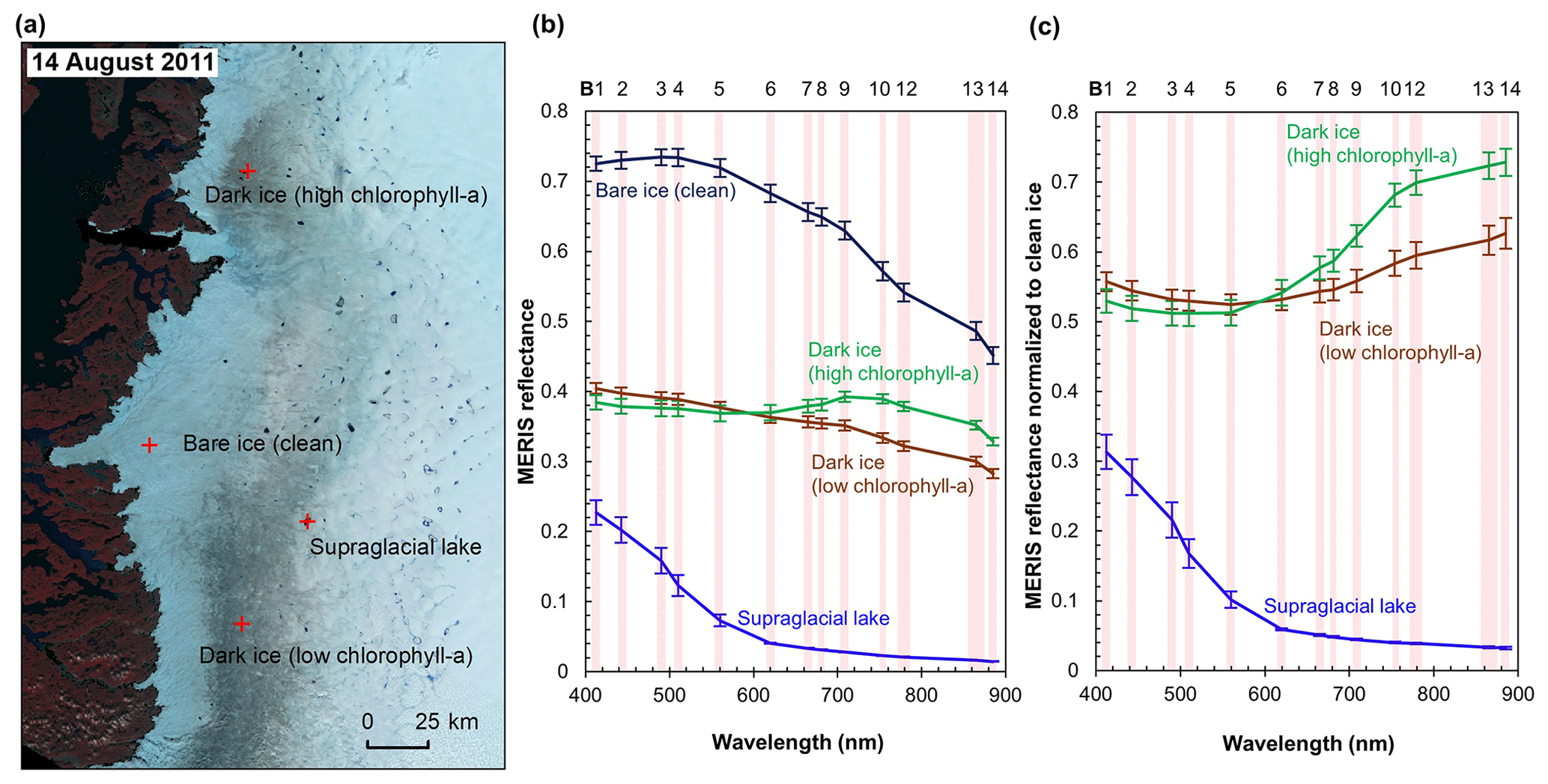
Figure 3MERIS spectra of different surface types. (a) MERIS Level-2 image (false color composite) acquired on 14 August 2011 and locations of the four sample sites. Each site has an area of 1.2 km × 1.2 km composed of 16 MERIS pixels. (b) MERIS reflectance in 13 spectral bands over the four sites, illustrated by mean and SD values for each band over each site. (c) Normalized reflectance relative to the clean ice spectra.
Table 2Calculated ratio indices and surface reflectance at 620 nm over the four sites.

3.3 Sensitivity analysis based on radiative transfer modeling
To evaluate the sensitivity of chlorophyll indices to dust presence, we performed radiative transfer modeling tests using the Snow, Ice, and Aerosol Radiation model (SNICAR; Flanner et al., 2007, 2009). SNICAR is a multilayer, two-stream radiative transfer model for simulating the spectral albedos of snow over the 300–5000 nm wavelength range (at a 10 nm spectral resolution), accounting for various factors including illumination conditions, snow grain size (30–1500 µm), snow layer properties, and dust concentrations, etc. The SNICAR online tool (available at http://snow.engin.umich.edu, last access: 1 February 2020) allows for simulating the radiative effects of dust in four size bins, in ranges of 0.1–1.0, 1.0–2.5, 2.5–5.0, and 5.0–10.0 µm. Dust optical properties in SNICAR are based on an estimate of global-mean characteristics approximated as a mixture of quartz, limestone, montmorillonite, illite, and hematite. We simulated the spectral albedos for varying sizes and concentrations of dust under the following conditions: direct incident radiation, a solar zenith angle of 60∘, clear sky conditions for Summit, Greenland, a snow grain effective radius of 1500 µm (approximating the ice surface), a snowpack thickness of 100 m, a snowpack density of 400 kg m−3, a range of dust concentrations (0.1, 0.3, 0.5, 0.8, 1, 1.5, 2, 2.5, 3, 5, 8, 10, 30, 50, 80, 100, 300, 500, 800, 1000, 1500, 2000, 2500, and 3000 ppm), and four dust sizes (dust 1: 0.1–1.0 µm; dust 2: 1.0–2.5 µm; dust 3: 2.5–5.0 µm; dust 4: 5.0–10.0 µm). We also tested different values of snow density (400 vs. 900 kg m−3) and found that the snow density value had a negligible effect on the simulation results. To evaluate the impact of snow grain size on the 2BDA index, we performed dust-free SNICAR simulations for different values of snow grain effect radius between 500 and 1500 µm (Fig. A1, Appendix A). We calculated the 2BDA index for each dust-free scenario, finding the lowest 2BDA value (0.959) for the 1500 µm spectra and the highest 2BDA value (0.976) for the 500 µm spectra. We compared these two 2BDA values with the histogram distribution of the 2BDA values calculated for the MERIS “clean” (R620 nm > 0.65) bare ice pixels (Fig. A1c). The sensitivity test suggests that the dust-free spectrum simulated using the 1500 µm grain size is a good approximation to the MERIS bare ice spectrum. Nevertheless, to account for the potential influence of grain-size changes on the sensitivity of 2BDA index to dust presence, we also repeated the SNICAR simulations with varying dust sizes and concentrations with a snow grain effective radius of 500 µm.
4.1 Comparison between different ratio indices
Figure 3 shows the MERIS spectra over four distinct sites within our study area to illustrate the spectra associated with different surface types. Each site represents a typical surface type, including clean bare ice, dark ice with a significant chlorophyll a signal, dark ice with a less significant chlorophyll a signal, and a supraglacial lake. Figure 3b shows that each surface type is characterized by a distinct spectral curve. The difference between the spectral curves for the two dark ice sites is particularly notable. Figure 3c shows the normalized spectral curves relative to the clean ice spectrum. Both of the dark ice sites have a reflectance at 620 nm of less than 0.47 and are classified as “dark ice” based on the thresholding method discussed above (Shimada et al., 2016; Tedstone et al., 2017). However, the northern dark ice site has a chlorophyll a spectral signature between 665 and 753 nm that matches the field spectra of algae-abundant ice (Fig. 2d), while at the southern dark ice site, the reflectance peak at 709 nm is much less pronounced. Since the magnitude of the chlorophyll a-related spectral signal is directly related to algae concentration, we termed the northern site as “dark ice (high chlorophyll a)” and the southern site as “dark ice (low chlorophyll a)” in Fig. 3 and Table 2. The differences illustrate that pixels classified as dark ice can have different spectral properties, and in particular differences associated with reflectance characteristics of chlorophyll a.
We calculated the 2BDA, 3BDA, NDCI, MCI, and impurity indices over bare ice (R865 nm < 0.53) for each MERIS image. Table 2 lists the ratio indices and the reflectance at 620 nm over the four sites shown in Fig. 3a based on a MERIS image acquired on 14 August 2011, to illustrate the differences between indices. The 2BDA, 3BDA, and NDCI chlorophyll a indices use similar spectral bands and are in general well correlated; they are highest over the northern dark ice site and lowest over the supraglacial lake. The MCI chlorophyll a index, in contrast, reaches a maximum over clean bare ice. The MCI index measures the height of the 709 nm reflectance peak relative to the baseline between 681 and 753 nm and is therefore sensitive to the bare ice spectrum. This index may be less sensitive to the relatively low chlorophyll a content over ice and is more suitable for monitoring intense algal blooms with very high chlorophyll a concentrations in water (Binding et al., 2013). For the impurity index, the clean bare ice has the lowest value, followed by the supraglacial lake; dark ice with the weaker chlorophyll a signal; and dark ice with the stronger chlorophyll a signal (Table 2). The supraglacial lake has a higher impurity index relative to clean ice, suggesting that the impurity index may include the darkening effect caused by meltwater presence. We find that the 2BDA, 3BDA, and NDCI indices are most suitable for detection of chlorophyll a, given their specificity to chlorophyll a signal bands, the sensitivity of the impurity index to liquid water, and the sensitivity of the MCI index to the bare ice spectrum. Of these three indices, we selected the 2BDA index to characterize the glacier algae distribution, owing to its simplicity and effectivity.
4.2 Sensitivity of the 2BDA index to non-algal factors
Given that dust may change the spectral reflectance of bare ice and affect the 2BDA index, we analyzed the sensitivity of 2BDA index to dust presence based on the SNICAR simulations for varying dust sizes and concentrations. We should note here that there has been some discussion in past literature regarding hematite-rich dust (e.g., Tedesco et al., 2013; Cook et al., 2020), which could produce a different spectral response. However, the field study of Cook et al. (2020) found very low concentrations of such dust, and therefore we consider its impact to be negligible. Using the simulated spectra, we calculated the 2BDA and impurity indices for each dust size and concentration. Figure 4 shows the 2BDA index vs. impurity index calculated for the SNICAR simulations using a snow grain effective radius of 1500 µm (with circle diameters representing the magnitude of dust concentrations for four different dust sizes), along with the density scatterplots of impurity vs. 2BDA index calculated from the MERIS data. The SNICAR simulations show that the impurity index is more sensitive to dust than the 2BDA index. Figure 4 illustrates that the upper bound of the impurity index calculated from the MERIS data is around 1.0. This maximum value corresponds to a dust concentration of ∼ 500 ppm (for the 5.0–10.0 µm dust range), which is consistent with the measurements of Cook et al. (2020), who reported mean and maximum dust concentrations of 342 and 519 ppm, respectively, over a field site within the study area. However, SNICAR simulations indicate that an impurity index of 1.0 corresponds to a maximum 2BDA value of ∼ 0.99. Therefore, the presence of dust alone cannot explain the high 2BDA index values present in Fig. 4. This comparison suggests that for our study area, areas with a 2BDA index greater than 0.99 are not likely to be false positives caused by dust. We also repeated this analysis using a snow grain effective radius of 500 µm (Fig. A1d, Appendix A). We find that the snow grain size mainly affects the lower range of 2BDA values, while the higher 2BDA values are less affected by grain-size changes. For the 500 µm grain size scenario, 2BDA values higher than ∼ 0.995 remain unaffected (Fig. A1d). Thus, the high MERIS 2BDA values are insensitive to dust presence regardless of grain-size variations.

Figure 4Impurity index vs. 2BDA index for MERIS bare ice pixels (density scatterplot with colors indicating relative frequency), excluding missing data in our study area, between 2004 and 2011. Circles show impurity vs. 2BDA index from SNICAR simulations (with a snow grain effective radius of 1500 µm) with varying concentrations of dust (for four different dust sizes). The circle size corresponds to the dust concentration, and dashed lines show the polynomial regression for each of the different dust sizes.
Although the bare ice spectrum can also be affected by other factors such as air bubbles and meltwater presence, there is no evidence suggesting that these factors can generate the chlorophyll a-like spectral signature with a higher reflectance at 709 nm as compared with 665 nm. In fact, ice with different concentrations of air bubbles has a consistent spectral shape between 665 and 709 nm (Condom et al., 2018), and meltwater exhibits a similar pattern to ice at this wavelength range (Fig. 3b), with both the ice and water spectra characterized by a decreased reflectance from 665 to 709 nm. The sensitivity of the 2BDA index to glacier algae can be further demonstrated using the field dataset of Cook et al. (2020). Table B1 and Fig. B2 (Appendix B) indicate strong positive correlations between measured cell abundance and the 2BDA index calculated from coincident in-situ hyperspectral data, particularly for those samples with a measured cell abundance of greater than 10 000 cells mL−1, which have an average 2BDA index of 1.09 ± 0.073. In comparison, the samples with a measured cell abundance of lower than 10 000 cells mL−1 have an average 2BDA index of 0.98 ± 0.015.
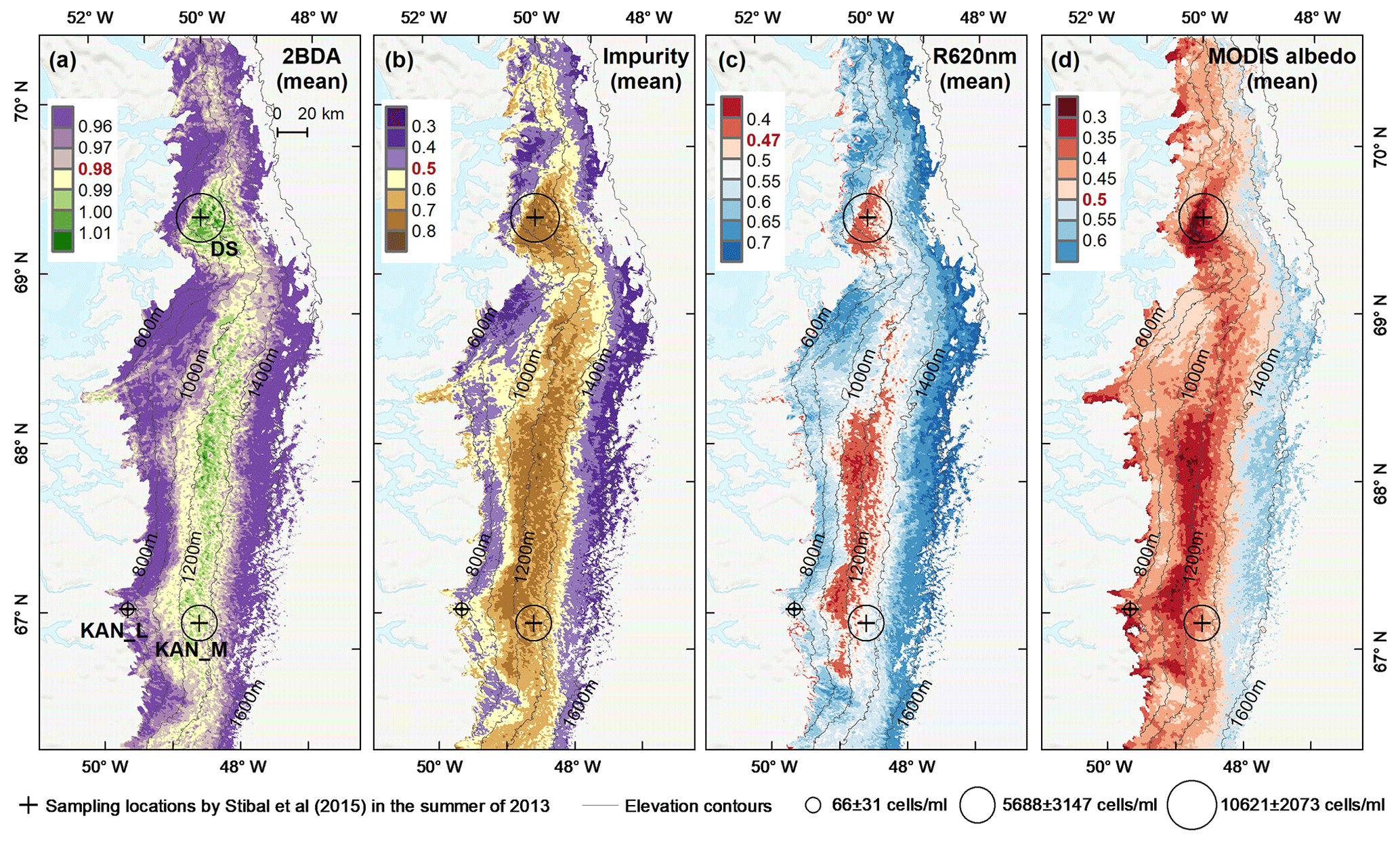
Figure 5Spatial patterns of the mean 2BDA index (a), impurity index (b), reflectance at 620 nm (c), and MODIS broadband albedo (d) over the bare ice zone during July and August from 2004 to 2011. The elevation contours illustrate the spatial variations of each variable with altitude. The cross labels show the spatial locations of the field sites DS, KAN_L, and KAN_M and magnitude of glacier algal abundance (circle labels) measured by Stibal et al. (2015) in 2013.
4.3 Spatial variability
To examine spatial variability on a broader scale, Fig. 5 shows the spatial patterns of the mean 2BDA index, impurity index, reflectance at 620 nm, and MODIS broadband albedo for the bare ice zone in our study area, averaged over 135 d when MERIS images are available between 2004 and 2011. Figure 5a, which shows patterns of the 2BDA index, suggests glacier algae are abundant at the DS region close to the Jakobshavn Isbrae Glacier between the altitudes of 600 and 1200 m and in the middle ablation area (68.5–66.5∘ N) between 1200 and 1400 m. These patterns are consistent with glacier algal maps derived from Sentinel-3 OLCI data for the 2016 and 2017 summer season (Wang et al., 2018). The relative magnitude of the 2BDA values between the DS, KAN_L, and KAN_M sites also matches the relative magnitude of field measurements of glacier algal abundance (Stibal et al., 2015; circles on Fig. 5), with the highest 2BDA index and algal abundance at the DS site, a lower value at the KAN_M site, and the lowest value at the KAN_L site.
A comparison between Fig. 5a and b and an examination of variation of the indices with elevation (Fig. A2, Appendix A) indicate a similarity in the spatial distribution of the two indices but also show notable differences. In particular, the 2BDA index reaches a peak at an elevation of 1300 m, while the impurity index peaks at 1180 m. As suggested by our sensitivity analysis discussed in Sect. 4.2, the 2BDA index is primarily sensitive to chlorophyll a, while the impurity index is sensitive to materials that darken the electromagnetic spectrum in visible wavelengths, including abiotic impurities (e.g., outcropping particulates; Wientjes et al., 2012), biological impurities, and liquid water. The map of reflectance at 620 nm, the band commonly used to delineate dark ice using a threshold (determined to be 0.47 for MERIS), is shown in Fig. 5c. Similar to the impurity index, the 620 nm reflectance and MODIS broadband albedo (Fig. 5d) reach a minimum value at 1180 m in elevation (Fig. A2; Fig. 5d). Comparison between the three indices and MODIS albedo suggests that algal abundance is highest between 1200 and 1400 m in elevation, contributing to reduced albedo, while other factors may play a more important role in albedo reduction at lower elevations. In particular, the darkening in some areas between 1000 and 1200 m in elevation could be attributed to longer exposure of bare ice resulting in increased consolidation of particulates with melt (Tedesco et al., 2016), where “wavy” patterns of outcropping dust can be observed (Wientjes and Oerlemans, 2010; Fig. A3, Appendix A). In contrast, imagery (WorldView-2) suggests that these wavy patterns may not be present at higher elevations where the appearance of dark material is more consistent with distributed algal material (Fig. A3). Other factors that may contribute to a reduction in MODIS albedo include liquid water and surface crevasses (e.g., Ryan et al., 2018), though their fraction is small relative to other surface types (Ryan et al., 2018).
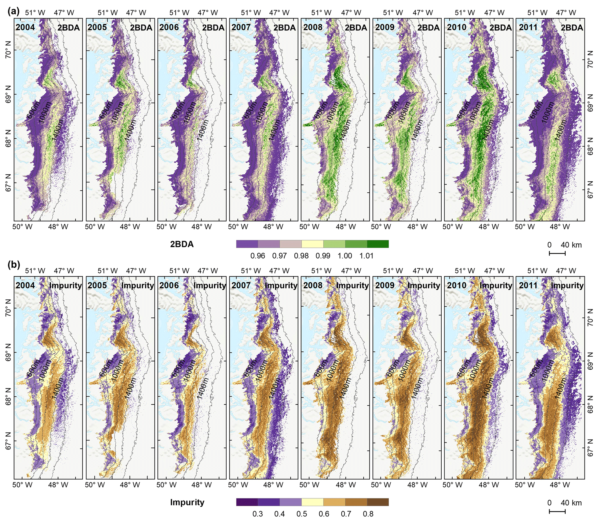
Figure 6Maps of mean 2BDA index (a) and impurity index (b) over July and August from 2004 to 2011.
4.4 Interannual variability
The annual time series (July–August mean) of the 2BDA index (Fig. 6a) and the impurity index (Fig. 6b) show the interannual variability of algal abundance and impurity content, indicating a general increasing trend in bare ice area, algal abundance, and total impurity content between 2004 and 2011, particularly after 2006. The spatial extent of glacier algae also expanded towards higher elevations (1200–1400 m) over this period. Between 2004 and 2011, the 2BDA index reached a maximum in 2010 when high air temperatures and intensive surface melt occurred over Greenland (Tedesco et al., 2011). The impurity index exhibits similar interannual variability compared with the 2BDA index but also exhibits different spatiotemporal variations between 1000–1200 and 1200–1400 m in the middle ablation area. Figure A4 (Appendix A) illustrates the interannual variability of the average 2BDA and impurity indices at different elevation levels (600–800, 800–1000, 1000–1200, and 1200–1400 m). In particular there are notable differences in variability of the 2BDA index between the 1000–1200 and 1200–1400 m levels. The interannual variability of the 2BDA and impurity indices is also coherent with variability in Greenland ice sheet-wide summer albedo, which was lowest in 2010 and highest in 2006 for the period 2004–2011 (Tedesco et al., 2018).
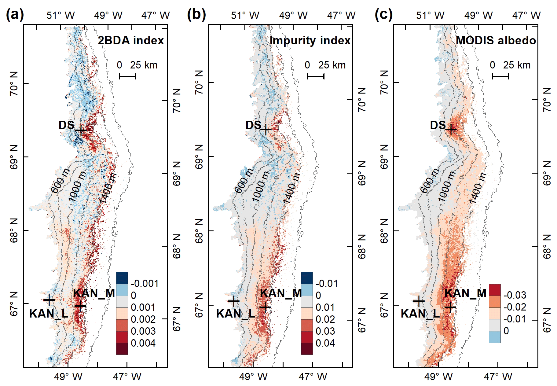
Figure 7Interannual trends (regression coefficients with year) of the 2BDA index (a), impurity index (b), and MODIS albedo (c) from 2004 to 2011.
We also calculated interannual trends in the 2BDA index, impurity index, and MODIS broadband albedo using linear regression analysis, with the mean 2BDA index, impurity index, or MODIS albedo for each year as the dependent variable and the year as the independent variable. Pixels with observations during fewer than 5 years were discarded from the analysis. Figure 7 shows the regression coefficients for 2BDA and impurity indices and MODIS albedo vs. time. The corresponding R2 and p-value estimates are shown in Fig. A5 (Appendix A). There were two primary regions within our study area that exhibited significant increases in algal abundance from 2004 to 2011 (Fig. 7a), the DS region in the north and the southern region (68.5–66.5∘ N) between 1200 and 1400 m in elevation. Other areas do not show statistically significant trends. The interannual trend of the impurity index (Fig. 7b) shows a larger spatial extent with a significant increasing trend as compared with the 2BDA index. Figure 7c shows that the areas with increasing algal abundance and increasing impurity index also had significant albedo (July–August mean) reduction from 2004 to 2011. The albedo reduction was roughly −0.025 to −0.04 per year over the K-transect area (between 1200 and 1400 m in elevation) and within the DS area. The spatial patterns of declining albedo more closely resemble the patterns of impurity index as opposed to the 2BDA index, suggesting that the impurity index quantifies multiple processes related to surface darkening in addition to glacier algae.
4.5 Seasonal trends of algal growth over July and August
To better understand seasonal dynamics of glacier algae, we examined intra-annual trends in the 2BDA index during the months of July and August. We estimated the temporal trend of the 2BDA index from July to August for each MERIS pixel. For each pixel and each day, we calculated the average 2BDA index using the same-day 2BDA indices of multiple years. To account for the differences between different years, we applied a temporal smoothing function with a window size of 3 d to the daily average 2BDA data. Pixels with more than 15 d of observations were kept for linear regression analysis, with the daily 2BDA index as the dependent variable and the time (in d) as the independent variable.
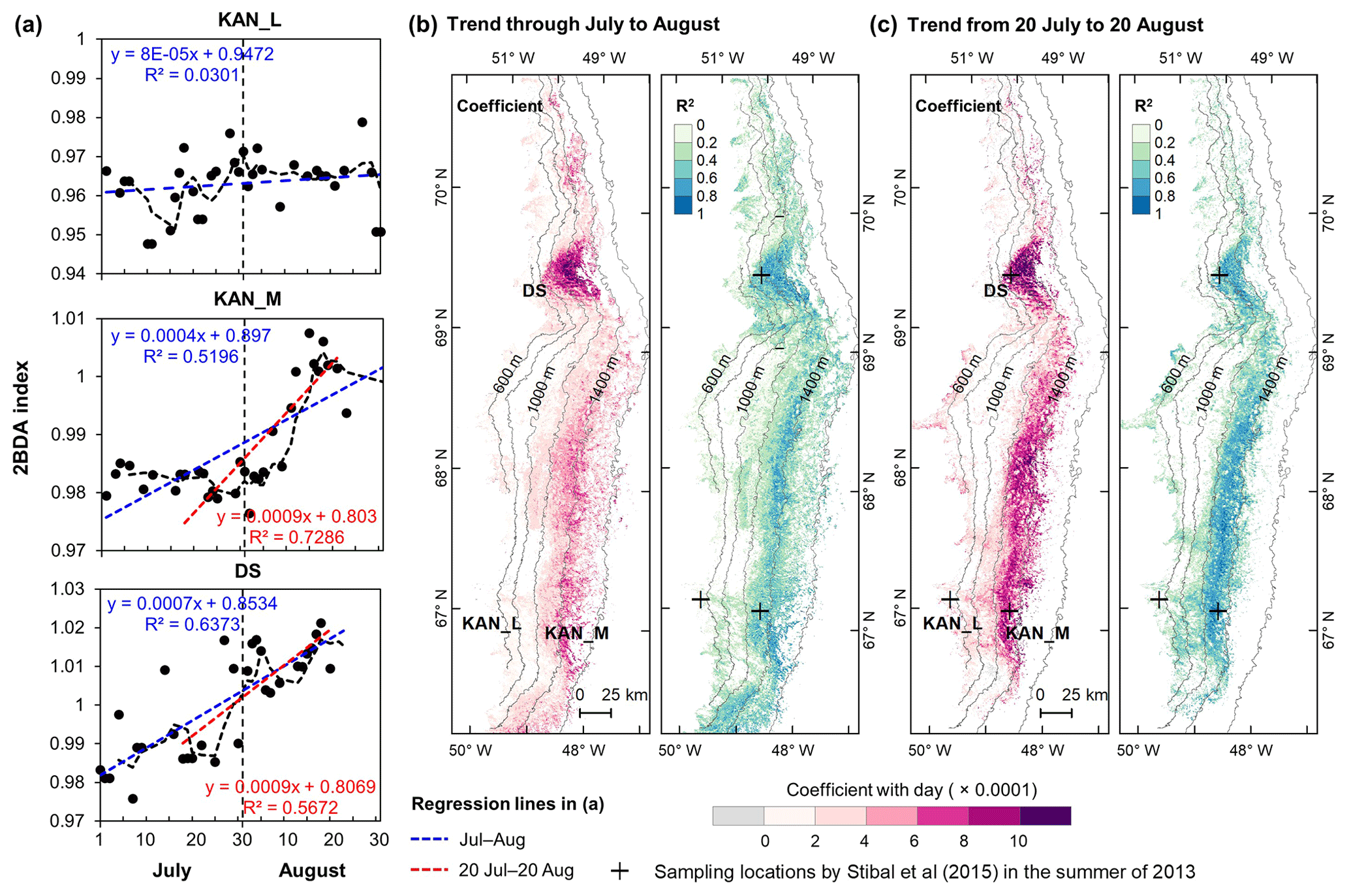
Figure 8Temporal trends of the 2BDA index over July and August. (a) The 2BDA time series and temporal trend analysis over the KAN_L, KAN_M, and DS sites. (b) Regression slope and R2 estimates of the temporal trend analysis for the period of July–August (for areas where the p value < = 0.05). (c) Regression slope and R2 estimates of the temporal trend analysis for the period of 20 July–20 August (for areas where the p value < = 0.05).
Figure 8 illustrates the pattern of seasonal trends across the southwestern Greenland ablation area. Figure 8b and c show the spatial distribution of seasonal trends across the area, while Fig. 8a shows examples of the daily 2BDA time series at the three field sites KAN_L, KAN_M, and DS. At the coastal KAN_L site, which had the lowest algal cell concentration (66 ± 31 cells mL−1), the average 2BDA index is less than 0.98 during July and August, and there is no significant temporal trend. At the KAN_M and DS sites, with higher cell concentrations (5688 ± 3147 and 10 621 ± 2073 cells mL−1, respectively), 2BDA values were mostly greater than 0.98, and there were significant increases in the 2BDA index during July and August (of 0.0004 and 0.0007 d−1, respectively), suggesting dramatic algal growth. The results indicate that the higher concentrations of algae are associated with a significant increasing trend over the course of a season. Indeed, the highest seasonal trends in the middle ablation area (68.5–66.5∘ N) are found in the 1200 to 1400 m elevation band, also the region of highest 2BDA index.
The time series in Fig. 8a suggest that the period of algal growth at KAN_M occurred primarily between mid-July and mid-August, beginning later than at the DS site. Between 20 July and 20 August, the regression slope was 0.0009 d−1 for both DS and KAN_M. This time window is consistent with the rapid algal colonization observed in field (Stibal et al., 2017; Williamson et al., 2018; Yallop et al., 2012; Lutz et al. 2018) and the patterns of temporal variability derived from Sentinel-3 data (Wang et al., 2018). To test whether higher growth rates later in the season were present across the region, we also examined region-wide trends between 20 July and 20 August (Fig. 8c). The magnitude of trends for the shorter period are higher over a broad region, and R2 values are higher, indicating a shorter growth period across much of the region, with the exception of the area around the DS site in the north. We also explored the interannual variability of seasonal patterns over the DS and KAN_M sites (Fig. A6, Appendix A). Despite the interannual variations of 2BDA index, the regression slopes of 2BDA vs. time (day) through mid-July to mid-August for different years were comparable to the slope of the aggregated time series between 2004 and 2011, particularly for the KAN_M site. Over the DS site, the algal growth rates were above average during the growth seasons in 2005, 2009, and 2011 (Fig. A6). The DS site is located in lower elevations, where warmer temperatures may promote a faster growth rate.
4.6 Impact of glacier algal blooms on surface albedo in July and August
To investigate the potential impact of algal changes on albedo variability, we quantified the relationship between glacier algal blooms and surface albedo in July and August based on the daily time series data of the 2BDA index and MODIS broadband albedo. A daily albedo time series obtained by averaging and smoothing the MODIS daily albedo data from 2004 to 2011 was derived using the same method for deriving the 2BDA seasonal trends. Figure 9 shows the derived temporal trends in MODIS albedo from 1 July to 20 August. The days after 20 August were excluded from the analysis since snowfalls often happen in late August. The DS area had the most significant albedo reduction over July and August, up to 0.004 ∼ 0.006 d−1. In the middle ablation zone between the altitudes of 1000 and 1200 m the albedo reduction rate was 0.002 ∼ 0.004 d−1, and the reduction rate was 0.002 ∼ 0.003 d−1 in the zone between 1200 and 1400 m in elevation.
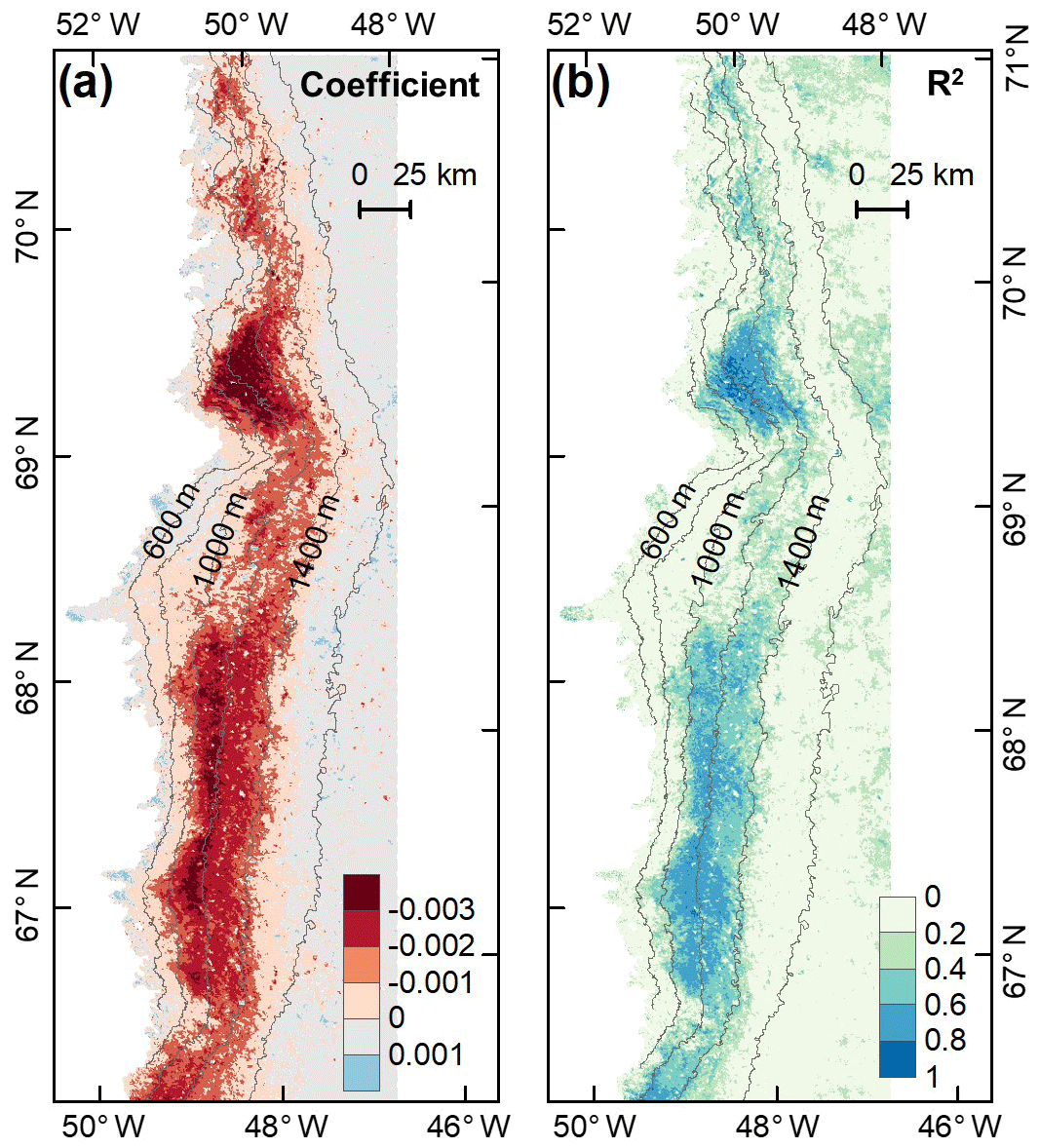
Figure 9Temporal trends in MODIS broadband albedo during July and August (over 2004–2011). (a) Regression coefficients of surface albedo with time (d) from 1 July to 20 August. (b) Corresponding R2 estimates.
We analyzed the relationship between surface albedo reduction and algal growth using the time series data of MODIS broadband albedo and the MERIS 2BDA index. Figure 10 shows the results of regression analysis with MODIS albedo as the dependent variable and the MERIS 2BDA index as the independent variable. The analysis indicates a statistically significant correlation between algal growth and albedo decrease at the DS area between the altitudes of 800 and 1200 m, the middle ablation zone between the altitudes of 1200 and 1400 m, and the 1000–1200 m area near the K-transect. Over these areas, the regression coefficient ranged from −4 to −2. Given the temporal rate of change of 2BDA index of 0.001 d−1 (Sect. 4.5), the surface albedo decreases by 0.002–0.004 d−1 in association with glacial algal growth. Figure 10 shows that algal growth can generally explain the temporal decrease in surface albedo during July and August in areas with significant albedo trends (Fig. 9), except in a portion of the middle ablation zone between the altitudes of 1000 and 1200 m where the correlation is less significant and other factors likely contribute to the observed albedo reduction.
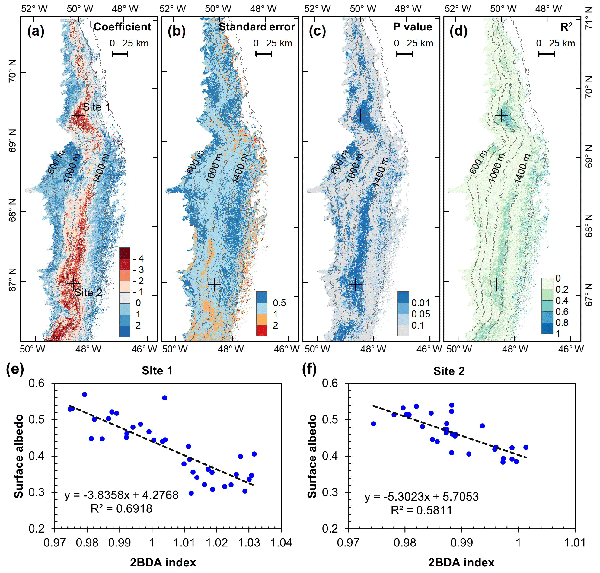
Figure 10Relationship between surface albedo and 2BDA index: (a) regression coefficients, (b) Standard errors of the correlation coefficients, (c) p values, and (d) R2 values. Panels (e, f) show surface albedo vs. 2BDA index at Site 1 and Site 2, respectively.
5.1 Sensitivity to subpixel variability
In this study, we utilized the chlorophyll a signal generated by glacier algae in the red–NIR region (Fig. 2d) to quantify the spatiotemporal variability of glacier algae at a regional scale for the summer seasons of 2004–2011 in southwestern Greenland. The specific wavelengths and narrow bandwidths of MERIS designed for chlorophyll a detection make MERIS archive data a powerful tool for studying supraglacial algal communities. The chlorophyll a signal present in the MERIS spectra is consistent with (nearly) coincident WorldView-2 data and hyperspectral field measurements collected over dark ice with high algal abundance (Fig. 2d). Similar to the Sentinel-3 OLCI ratio index R709 nm∕R673 nm, the MERIS 2BDA index R709 nm∕R665 nm can effectively quantify the algal growth pattern during July and August (Fig. 8). Using SNICAR simulations, we examined the potential impact of dust on the 2BDA index. The comparison between SNICAR simulations and MERIS ratio indices indicates a high sensitivity of the 2BDA index to glacier algae as compared to dust (Fig. 4). Here we explore the sensitivity of the 2BDA index to subpixel variability using a linear mixing method based on the field spectral measurements of Cook et al. (2020) and the SNICAR-simulated spectra for dust (size 4 with a concentration of 500 ppm, snow grain effective radius as 1500 µm). The spectra used for linear mixing experiments are shown in Fig. B3a (Appendix B). By specifying the areal percentage of the impurity-covered (algae or dust) surface at subpixel scale, we calculated the mixed spectra by linearly combining the algae (four samples with different measured algal abundance) or dust spectra (SNICAR-simulated) with the bare ice spectrum (measured algal abundance of 0 cells mL−1) weighted by areal percentage. Figure B3b (Appendix B) shows the 2BDA index calculated from the mixed spectra varying with the areal percentage of algae or dust at the subpixel scale. It is shown that the 2BDA index dramatically increases with the areal percentage of glacier algae, being consistent with the positive correlation between the 2BDA index and algal abundance. In contrast, the 2BDA index is much less sensitive to dust areal coverage. The results indicate that even with sub-pixel variability of surface materials, the satellite-derived 2BDA index is still strongly sensitive to the presence of algae. High-resolution UAV mapping by Ryan et al. (2018) suggests that the areal percentage of distributed impurities is up to 65 %–95 % within individual MODIS pixels (500 m resolution) over the dark zone in southwestern Greenland, indicating that a high sub-pixel areal percentage of algae is possible. Our linear mixing experiments (Fig. B3b) indicate that the relatively high 2BDA values derived from satellite are unlikely to be achieved without the presence of glacier algae and that the MERIS 2BDA index can effectively capture the glacier algae variability, especially within the dark zone.

Figure 11(a) Comparison between MAR albedo and MODIS albedo over the study area for July and August from 2004 to 2011. The dashed line shows the linear fit between MODIS albedo and MAR albedo. The black line is the 1:1 reference line. (b) Relationship between the MERIS 2BDA index and the albedo difference between MODIS and MAR, with the dashed line showing the linear fit. The color scheme in both (a) and (b) illustrates the relative data distribution density (yellow means higher density, and blue means lower density).
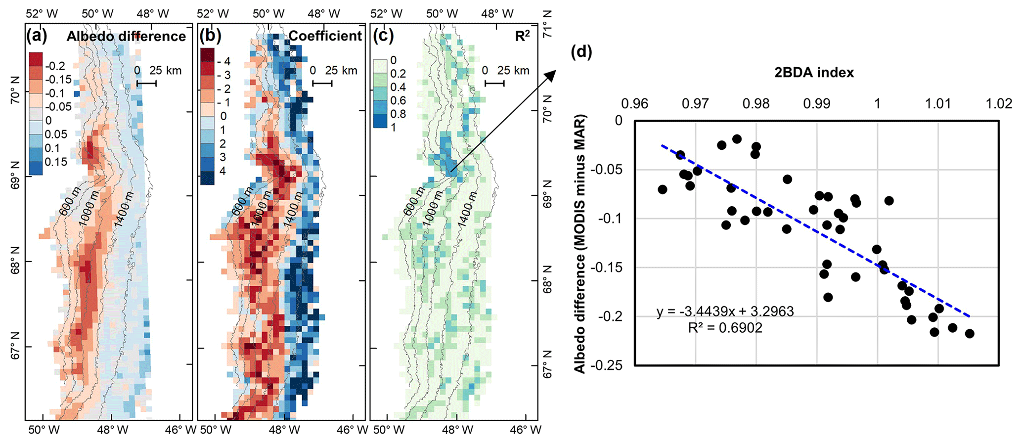
Figure 12(a) Albedo difference between MODIS albedo and MAR albedo (MODIS albedo minus MAR albedo) averaged over the study period. (b) Regression coefficients of albedo difference with 2BDA index. (c) R2 estimates for the regression analysis. (d) Scatterplot of albedo difference vs. 2BDA index over the DS algae-abundant area and the equation for the linear fit.
5.2 Relationship between regional climate model albedo bias and glacier algae
Our analysis suggests a strong negative correlation between surface albedo and 2BDA index during July and August primarily in algae-abundant areas close to the Jakobshavn Isbrae Glacier and within the middle ablation zone (68.5–66.5∘ N) between 1200 and 1400 m in elevation. It is also important to know whether the MERIS 2BDA index could explain the discrepancy between the satellite-measured albedo and bare ice albedo in climate models that do not currently simulate the effects of biology and other impurities. The MAR regional climate model, for instance, exhibits a positive albedo bias along the southwestern Greenland ice sheet margin because of this (e.g., Alexander et al., 2014). Figure 11a shows a comparison between MODIS albedo and MAR albedo over the study area (including both bare ice and snow), indicating the overestimation of MAR albedo for the dark areas with MODIS albedo less than 0.5. There is a significant negative correlation between the albedo difference (MODIS albedo minus MAR albedo) and the 2BDA index (Fig. 11b), indicating that the positive MAR albedo bias increases with algal abundance.
The spatial pattern of the MAR albedo bias (Fig. 12a) is consistent with the satellite-derived impurity distribution (e.g., Fig. 5b). Over the dark areas, the MAR albedo was overestimated by 0.16 ± 0.03 as compared to the MODIS albedo. We further examined the relationship between the albedo bias (MODIS albedo minus MAR albedo) and the 2BDA index for the seasonal trend between 1 July and 20 August, finding a significant correlation in the DS site region (Fig. 12b–d). Figure 12d shows that the albedo bias between MODIS and MAR has a significant negative correlation with the 2BDA index. The estimated regression coefficient is −3.4439. Combined with the estimated temporal trend in the 2BDA index over time of 0.0009 d−1 (Fig. 8), the algal growth can explain a −0.0031 daily change in the albedo bias between MAR and MODIS at the DS site. Assuming a growth season extending from 1 July to 20 August (51 d), algal growth can explain a total difference of −0.158 between MODIS and MAR albedos. In comparison, the albedo bias in the middle zone between 1000 and 1400 m is less well-explained by glacier algae. This is partially consistent with our previous analysis that the albedo reduction at 1000–1200 m is poorly related to algal growth. Between 1200 and 1400 m, the correlation between the 2BDA index and the MAR bias is not strong (Fig. 12c), even though there is a fairly strong correlation between the 2BDA index and MODIS albedo. This suggests that in this area, although MAR does not include the effects of algae, the decrease in albedo associated with liquid water ponding in MAR may approximate the trends associated with increasing algae concentrations. In addition to parameterizing glacier algal growth, other processes related to albedo reduction such as consolidation of impurities melted from snow should be also accounted for in the future.
5.3 Relationship between 2BDA index and algal population
In order to use remote sensing data to quantify the temporal change of algal population with time, it is necessary to establish an empirical relationship between 2BDA index and algal abundance. However, there are no field data for glacial algal abundance coincident with the MERIS operational period. In ocean color studies, the relationship between 2BDA index and chlorophyll a concentration is generally formulated as an exponential function or a linear function (Matthews, 2011; Gholizadeh et al., 2016). Wang et al. (2018) derived an exponential function relating the Sentinel-3 OLCI reflectance ratio R709 nm∕R673 nm and field data for glacier algal abundance (Stibal et al., 2015; Williamson et al., 2018) as follows:
where x denotes the reflectance ratio and y denotes the algal abundance (cells mL−1). Following from Eq. (3), the empirical relationship between algal abundance and 2BDA index can be represented in a general form as follows:
where x denotes the 2BDA index, y is algal abundance, b is the base number of the exponential function (e in Eq. 3), and a and c are the regression coefficients. The time for one algal population doubling (the number of algal cells has doubled) can be calculated as the reciprocal of , where t represents time. Based on Eq. (4) and derivative rules, can be represented as follows:
where is the rate of change of 2BDA with time, i.e., the regression coefficient from the temporal trend analysis of 2BDA index vs. time (Sect. 4.5; Fig. 8). Similarly, the relationship between surface albedo (α) and algal population doubling level (log2y) can be calculated using:
where is the regression coefficient of surface albedo α vs. 2BDA index (Sect. 4.6; Fig. 10).
Given the similarity between the OLCI and MERIS band configurations and the negligible differences between the 673 and 665 nm reflectance, we attempted to use Eqs. (3), (5), and (6) to calculate the algal population doubling time corresponding to various values of the regression coefficients of 2BDA vs. time, as well as the albedo change rate due to each algal population doubling corresponding to different regression coefficients of albedo vs. 2BDA. The results of these calculations are listed in Tables 3 and 4, respectively. According to Fig. 8c, the areas with significant algal growth trend (R2 > 0.5) between 20 July and 20 August had a mean regression coefficient of 0.00076 ± 0.0002, which corresponds to a mean algal population doubling time of 11.2 ± 2.6 d. The DS area had faster algal growth rate than other areas, which corresponds to a doubling time of 9.6 ± 2.7 d. Figure 10a indicates that the regression coefficient of albedo vs. 2BDA over the algae-abundant areas ranges between −4 to −2, corresponding to a surface albedo decrease of 0.032–0.016 for each algal population doubling. Although these values were inferred using the Sentinel-3-derived relationship and there are uncertainties (e.g., spectral mixing) associated with algal abundance quantification, it is notable that our derived doubling time and albedo impact estimates are comparable to previous field studies. Williamson et al. (2018) reported a doubling time of 7.18 ± 1.04 d for algae-abundant ice (at the K-transect) based on field data collected during the summer of 2016. Stibal et al. (2017) estimated a net albedo reduction of 0.038 ± 0.0035 for each algal population doubling based on in-situ measurements of glacier algal abundance and coincident surface albedo. Despite the apparent agreement, further research is required to build a robust relationship between 2BDA index and algal abundance and also quantify the uncertainties caused by different factors.
Table 3Inferred algal population doubling time for given regression coefficients of 2BDA vs. time.
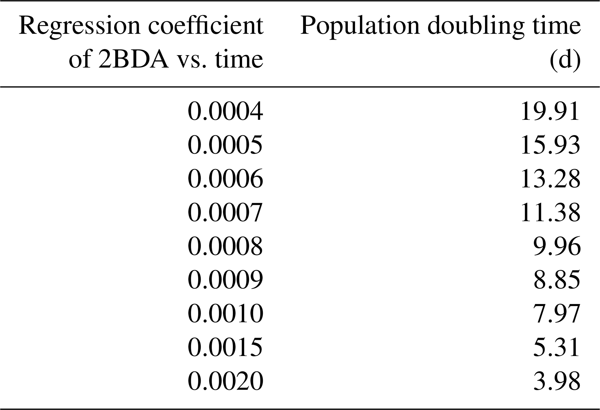
Table 4Inferred surface albedo change rate due to algal doubling given regression coefficients of albedo vs. 2BDA index.
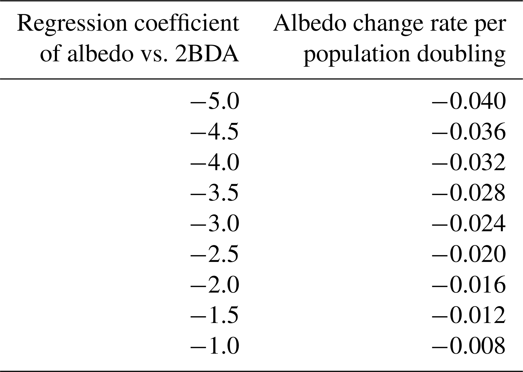
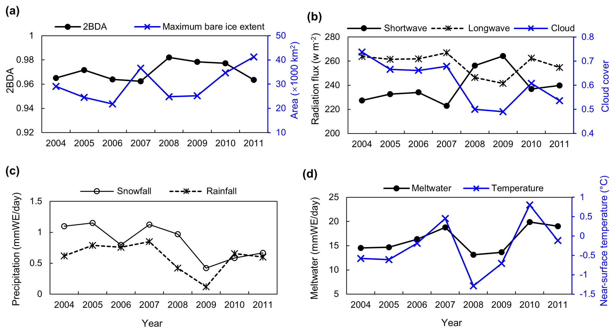
Figure 13(a) Average 2BDA index over bare ice and maximum bare ice area from 2004 to 2011 (MERIS). (b) July–August mean of downward shortwave and longwave radiation fluxes and cloud cover over the study area from 2004 to 2011 (MAR). (c) July–August mean of rainfall and snowfall (MAR). (d) July–August mean of meltwater production and near-surface temperature (MAR).
5.4 Potential drivers for glacier algae variability
Due to the impact of glacier algal blooms on bare ice albedo, it is fundamental to understand the factors affecting algal growth. Lutz et al. (2018) analyzed the composition of glacier algal communities near the K-transect between 27 July and 14 August 2016 using high-throughput sequencing and subsequent oligotyping techniques. The glacier algae species of Ancylonema nordenskiöldii and Mesotaenium berggrenii were found as the dominant taxa. Glacier algae lack a flagellated stage and are less capable of migrating upwards to snow layers at the beginning of melting season (Anesio et al., 2017). Therefore, glacier algal growth is restricted to the bare ice surface, which is consistent with our finding that glacier algal blooms tend to occur extensively from late-July to mid-August when the bare ice is exposed. However, somewhat paradoxically, the areas at lower altitude have a longer duration of bare ice exposure, whereas intense glacier algal blooms occur at higher altitude up to 1200–1400 m along the middle ablation zone. One possible reason for this discrepancy could be that the growth of glacier algae is influenced by liquid water (e.g., Tedstone et al., 2017) and nutrient availability. Although liquid water is a prerequisite for algal growth, Wang et al. (2018) found a negative correlation between algal abundance and meltwater production, which was attributed to hydrological flushing of algae during periods of excessive meltwater and surface runoff (Takeuchi, 2001; Uetake et al., 2010). These results do not contradict the importance of liquid water to algal growth as indicated by Tedstone et al. (2017), but rather suggest that there is an optimal amount of melt that may be required to support algal growth, with too little or too much melt resulting in lower algal concentrations.
To examine potential drivers of algal growth, we explored the relationships between the 2BDA index and topographic variables as well as near-surface temperature and meltwater production simulated by MAR (Fig. C1, Appendix C), by separating the data into two-dimensional bins and calculating the average 2BDA index for each bin. The comparison suggests that glacier algae are mostly distributed over flat areas with fewer topographic undulations (Fig. C1a). The areas suitable for glacier algal growth have moderate but not excessive melting (Fig. C1b). This further supports the hypothesis that high melt has a negative effect on algal development. In regard to the suitable temperature, glacier algae are so far known to be well-adapted to temperatures close to 0 ∘C (Anesio et al., 2017). Although no significant correlations have been found between algal abundance and air temperature, Figure C2 (Appendix C) shows dips in measured daily algal abundance (Stibal et al., 2017) coinciding with below-freezing near-surface MAR-simulated daily air temperatures at the K-transect S6 station during the 2014 summer, suggesting that freezing temperatures negatively impact algal growth.
We also examined interannual variations in climate variables in relation to the 2BDA index. Figure 13 shows the MAR-simulated shortwave and longwave downward radiation fluxes, cloud cover, snowfall, rainfall, meltwater production, and near-surface air temperature averaged over July and August across the study area from 2004 to 2011. The high 2BDA algal index during 2008–2010 (Figs. 5a and 13a) coincides with reduced cloud cover and higher incoming shortwave radiation (Fig. 13b). This period is also characterized by less rainfall (Fig. 13c), reducing the possibility of hydro-flushing. Figure 13d shows that the high algal index years of 2008 and 2009 exhibited less melting and lower temperature than the other years, suggesting that these variables may play a less important role in algal growth than shortwave radiation. Given the importance of shortwave radiation for photosynthesis of glacier algae, the results suggest that air temperature, surface melt, and bare ice exposure may be important factors at the beginning stage of glacier algal habitat development, while downward shortwave radiation could be most important during the proliferation stage. These dynamics could be influenced by recent atmospheric circulation changes in Greenland, with patterns of anomalous anticyclonic circulation and higher 500 hPa geopotential height becoming more frequent (e.g., Hanna et al., 2016; Mioduszewski et al., 2016), associated with reduced cloud cover (Hofer et al., 2017) and increased downward shortwave radiation. However, more research is required to fully understand these relationships and quantify the effects of various factors on glacier algal growth. In the context of future ice sheet change, it is therefore vital to understand the interactions between the supraglacial microbiome and climate change (Cavicchioli et al., 2019) for better projection of future ice sheet mass balance.
We examined the spatiotemporal variability of glacier algal blooms in southwestern Greenland during July and August from 2004 to 2011 using the chlorophyll a detection capability of MERIS. We calculated a number of remote sensing ratio indices, including chlorophyll a indices and the impurity index. The results indicate that, similar to the Sentinel-3 OLCI ratio index of R709 nm∕R673 nm, the MERIS 2BDA index of R709 nm∕R665 nm can effectively quantify the spatial distribution and seasonal growth pattern of glacier algae, with results highly consistent with field measurements. There was an increasing trend of glacier algal abundance and impurity content within the dark area close to Jakobshavn Isbrae Glacier and the area close to the K-transect at an altitude of 1200–1400 m, in conjunction with a declining trend of surface albedo over the 2004 to 2011 period. We quantified the impact of glacier algal growth on surface albedo over July and August, and found significant correlations between albedo reduction and algal growth over algae-abundant areas. Our analysis points to the great potential of using satellite ratio indices to parameterize the impact of glacier algae on surface albedo, thereby reducing the albedo bias in regional climate models. Nevertheless, the surface darkening along the middle ablation zone between 1000 and 1200 m in elevation cannot be well explained by algal growth, indicating that other processes related to surface darkening need further investigation and quantification. Future research should also be directed toward understanding the climate drivers of glacier algae variability and parameterizing their growth dynamics in regional climate model simulations.
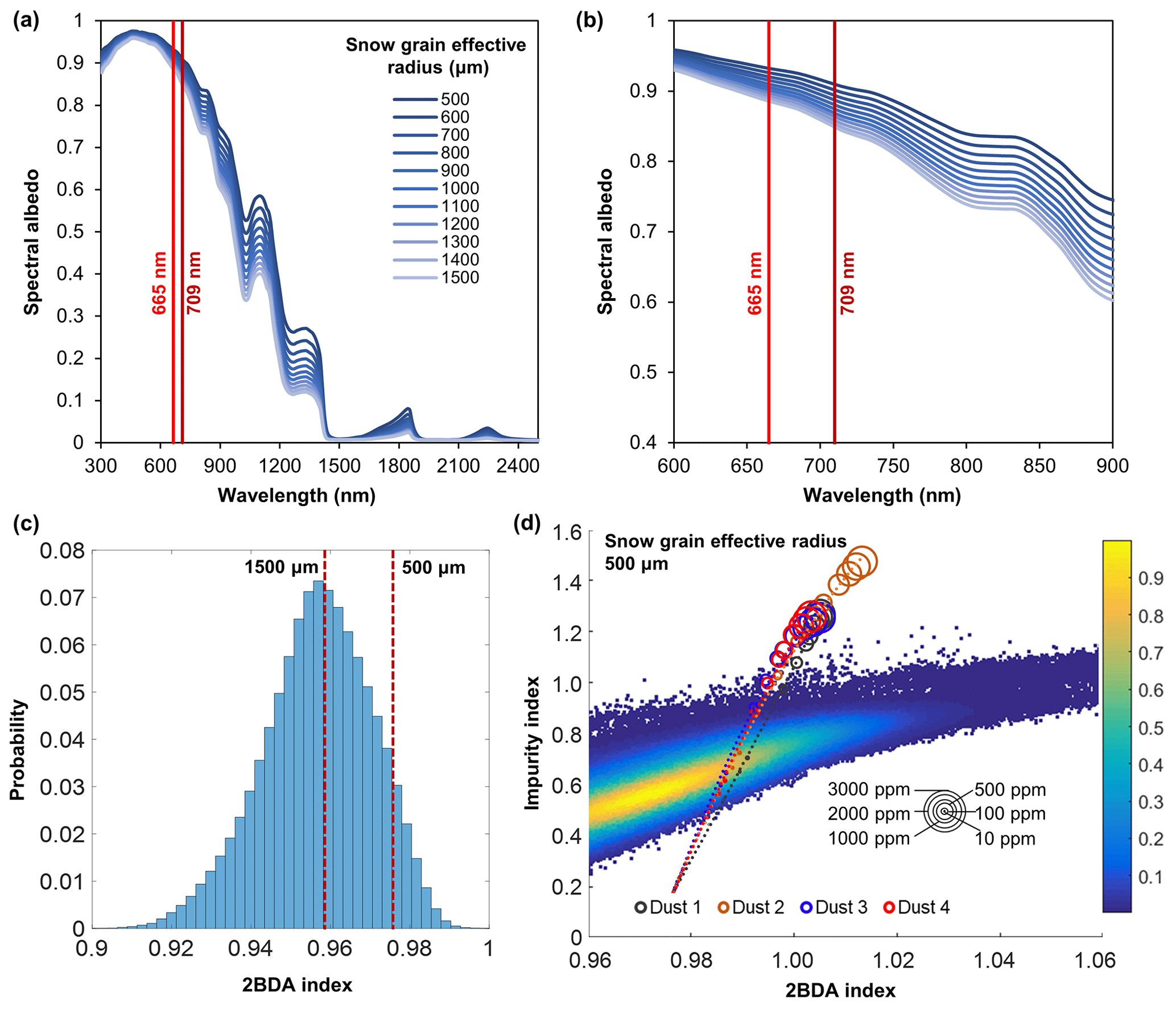
Figure A1(a) SNICAR dust-free simulations for different snow grain sizes (500–1500 µm). (b) Zoomed-in graph of (a) showing details of spectral albedo values at 665 and 709 nm. (c) Histogram of the 2BDA index for MERIS bare ice pixels with 620 nm reflectance greater than 0.65 (clean ice) and the corresponding 2BDA values for the SNICAR dust-free simulations with snow grain size of 500 and 1500 µm. (d) Impurity index vs. 2BDA index for MERIS bare ice pixels (density scatterplot with colors indicating relative frequency) and for SNICAR simulations (circles and dashed lines) with snow grain size of 500 µm for varying concentrations of dust (four different dust sizes). The circle size corresponds to the dust concentration, and dashed lines show the polynomial regression for each of the different dust sizes.
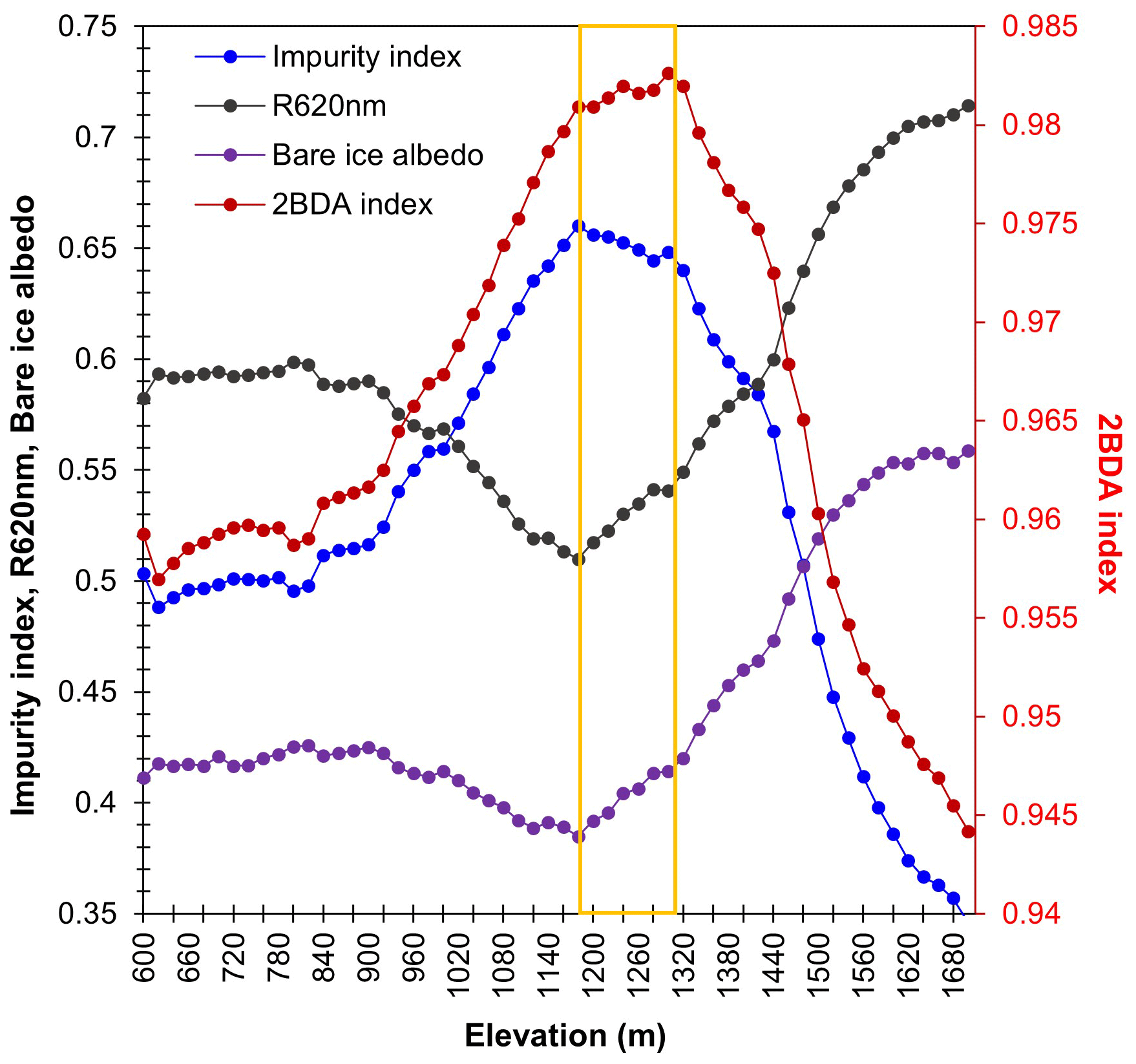
Figure A2Spatial variations of the average 2BDA index, impurity index, 620 nm reflectance, and MODIS albedo over bare ice at different elevations within the study area (20 m elevation interval). For surface elevation, we used the 30 m resolution MEaSUREs Greenland Ice Mapping Project (GIMP) Digital Elevation Model (Howat et al., 2014, 2015).
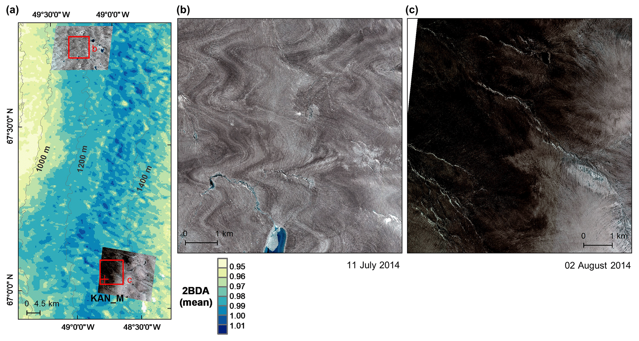
Figure A3Average 2BDA index (2004–2011) for a subset of our study area (a), and comparison between WorldView-2 imagery (© 2014 DigitalGlobe, Inc.) over a dark ice site with low 2BDA index at 1000–1200 m elevation (b) and a dark ice site with high 2BDA index at 1200–1400 m elevation (c). The WorldView-2 image in (b) illustrates the wavy pattern that Wientjes and Oerlemans (2010) suggested was caused by ancient ice outcropping. The WorldView-2 images are radiometrically calibrated (top-of-atmosphere radiances) and orthorectified and are shown as a true color composite (red channel: 659 nm band; green channel: 546 nm band; blue channel: 478 nm band).
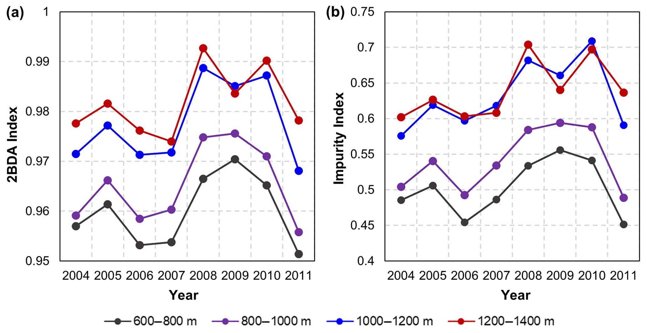
Figure A4Interannual variability of the 2BDA index (a) and impurity index (b) at the elevation levels of 600–800, 800–1000, 1000–1200, and 1200–1400 m within the study area.
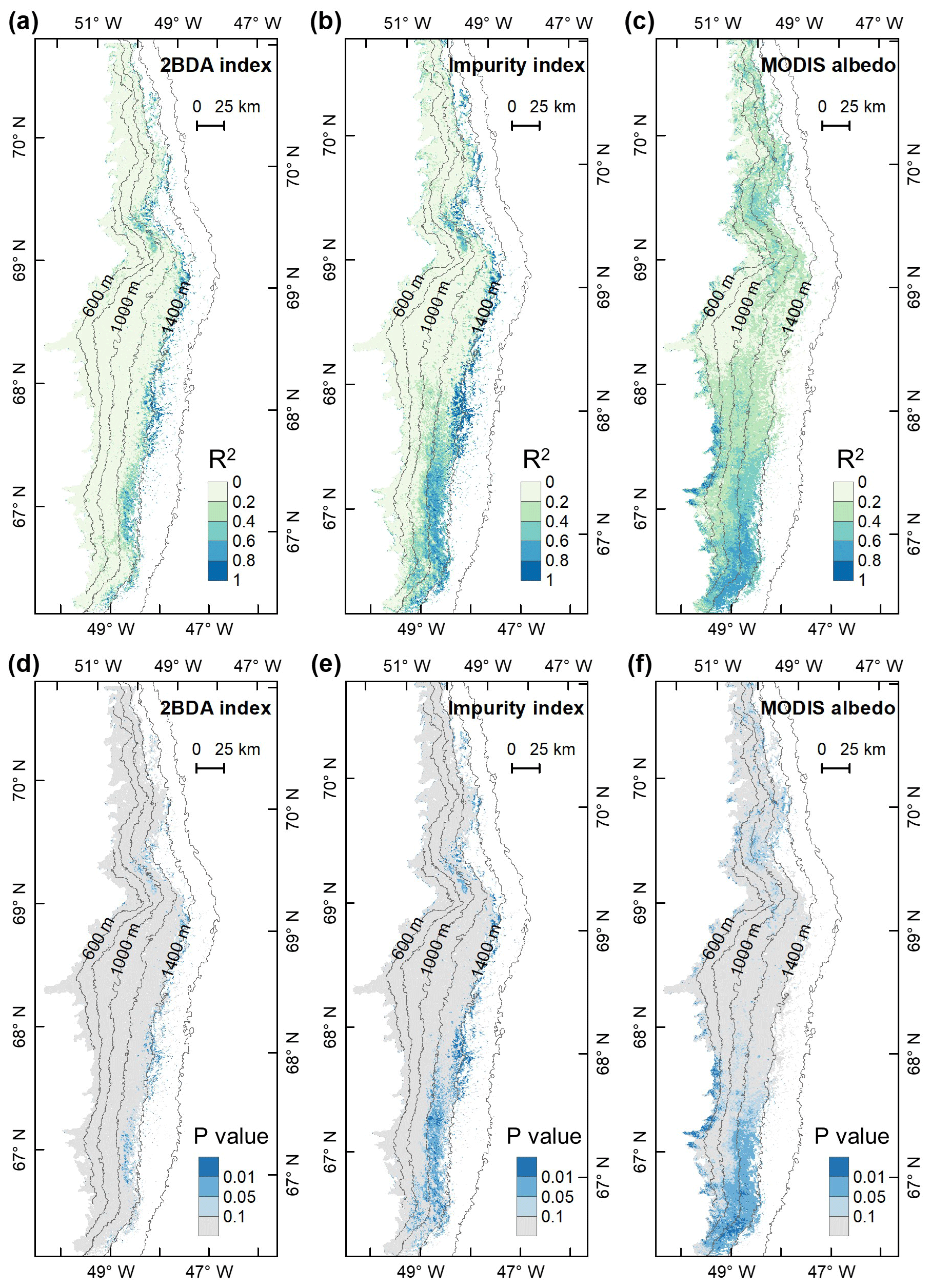
Figure A5R2 and P values for the interannual trends of the 2BDA index, impurity index, and MODIS albedo from 2004 to 2011.
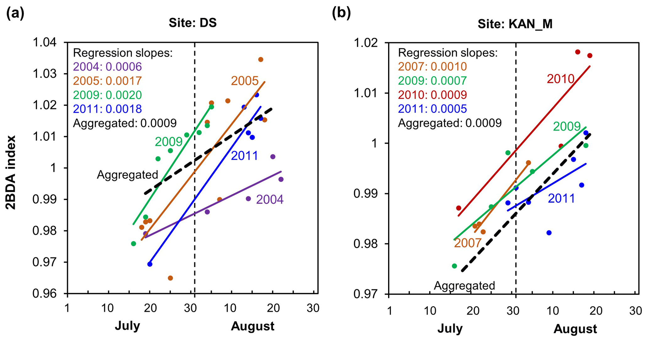
Figure A6Temporal trends of 2BDA index from mid-July to Mid-August in different years at sites DS (a) and KAN_M (b).
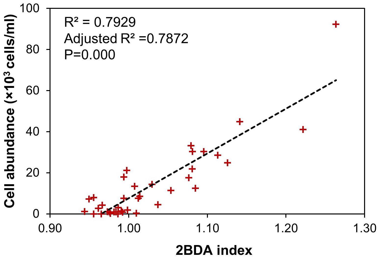
Table B1Measured algal cell abundance from the field dataset of Cook et al. (2020) with the 2BDA index calculated from coincident hyperspectral measurements. The highlighted rows in bold are samples with cell abundance of greater than 10 000 cells mL−1.

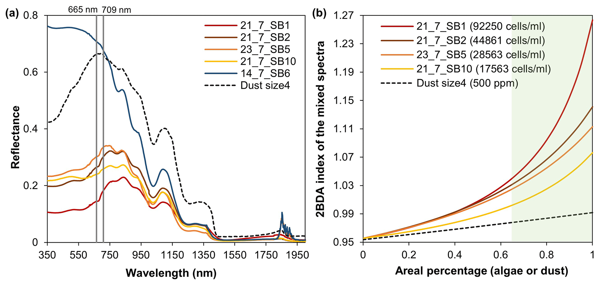
Figure B2Spectral linear mixing experiments. (a) Field hyperspectral measurements of four algae-abundant samples (21_7_SB1, 21_7_SB2, 23_7_SB5, and 21_7_SB10) and one bare ice sample (zero algal abundance, 14_7_SB6) from Cook et al. (2020), and the SNICAR-simulated spectra for the dust scenario (size 4 at concentration of 500 ppm). (b) The 2BDA index calculated from the linearly mixed spectra with varying areal percentage at subpixel scale for algae (different algal abundances) and dust scenarios.

Figure C1(a) The 2BDA index vs. surface elevation and roughness (elevation variability within each MERIS pixel). (b) The 2BDA index vs. near-surface temperature and meltwater production simulated by MAR. The color bars in (a) and (b) indicate the average 2BDA index for each two-dimensional bin defined by the two variables on the horizontal and vertical axes.
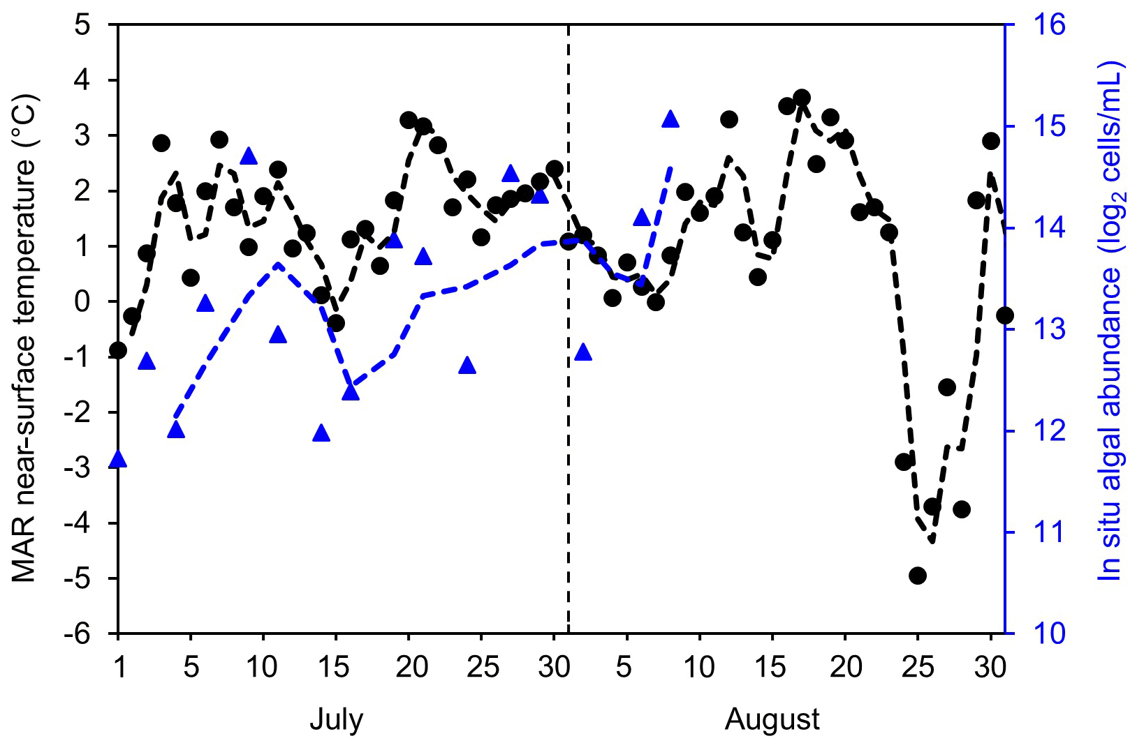
Figure C2MAR-simulated near-surface air temperature (∘C, black circle, left axis) and in situ measured algal abundance (log2 cells mL−1, blue triangles, right vertical axis) at the S6 weather station at the K-transect during July–August 2014 by Stibal et al. (2017).
MERIS level-2 data are available at the MERCI file archive (https://merisfrs-merci-ds.eo.esa.int/, last access: May 2019), courtesy of the European Space Agency. MODIS MOD09GA (https://doi.org/10.5067/MODIS/MOD09GA.006, Vermote and Wolfe, 2020) and MOD10A1 (https://doi.org/10.5067/MODIS/MOD10A1.006, Hall and Riggs, 2016) data can be accessed from the NASA Land Processes Distributed Active Archive Center (https://search.earthdata.nasa.gov/, last access: February 2020). MAR v3.9.3 outputs are available at ftp://ftp.climato.be/fettweis/.MARv3.9.3 (last access: April 2019).
SW, MT, and PA designed the study. SW processed the MERIS, MODIS, and WorldView-2 data. SW and MX tested the MERIS ratio indices. XF provided the MAR v3.9 outputs. SW, MT, and PA analyzed the results and generated figures. SW wrote the manuscript. All authors discussed the results and contributed to the final manuscript.
The authors declare that they have no conflict of interest.
This work was supported by National Science Foundation, NASA Exobiology program, NASA Modeling, Analysis, and Prediction (MAP) program, and the Heising-Simons foundation. We would like to thank the Polar Geospatial Center (https://www.pgc.umn.edu/, last access: 1 August 2019) for providing the WorldView-2 imagery, the European Space Agency for distributing the MERIS data, and the NASA Land Processes Distributed Active Archive Center and National Snow and Ice Data Center for distributing the MODIS data. Geospatial support for this work provided by the Polar Geospatial Center under NSF-OPP awards 1043681 and 1559691. Thanks to David Porter (Lamont-Doherty Earth Observatory, Columbia University) and Rafael Antwerpen (Utrecht University) for providing comments on the final manuscript. We also thank the editor and two anonymous reviewers for comments and suggestions that greatly improved the manuscript.
This research has been supported by the National Science Foundation (grant nos. ANS 1713072, PLR-1603331) and the National Aeronautics and Space Administration (grant nos. 80NSSC18K0814, 80NSSC17K0351, NNX17AH04G).
This paper was edited by Stef Lhermitte and reviewed by two anonymous referees.
Alexander, P. M., Tedesco, M., Fettweis, X., van de Wal, R. S. W., Smeets, C. J. P. P., and van den Broeke, M. R.: Assessing spatio-temporal variability and trends in modelled and measured Greenland Ice Sheet albedo (2000–2013), The Cryosphere, 8, 2293–2312, https://doi.org/10.5194/tc-8-2293-2014, 2014.
Anderson, G. P., Felde, G. W., Hoke, M. L., Ratkowski, A. J., Cooley, T. W., Chetwynd, J. H., Gardner, J. A., Adler-Golden, S. M., Matthew, M. W., Berk, A., Bernstein, L. S., Acharya, P. K., Miller, D. P., and Lewis, P. E.: MODTRAN4-based atmospheric correction algorithm: FLAASH (fast line-of-sight atmospheric analysis of spectral hypercubes), in: Algorithms and Technologies for Multispectral, Hyperspectral, and Ultraspectral Imagery VIII, vol. 4725, International Society for Optics and Photonics, 65–72, 2002.
Anesio, A. M., Lutz, S., Chrismas, N. A. M., and Benning, L. G.: The microbiome of glaciers and ice sheets, NPJ Biofilms Microbiomes, 3, 10, 2017.
Beck, R., Zhan, S., Liu, H., Tong, S., Yang, B., Xu, M., Ye, Z., Huang, Y., Shu, S., Wu, Q., Wang, S., Berling, K., Murray, A., Emery, E., Reif, M., Harwood, J., Young, J., Nietch, C., Macke, D., Martin, M., Stillings, G., Stump, R., and Su, H.: Comparison of satellite reflectance algorithms for estimating chlorophyll a in a temperate reservoir using coincident hyperspectral aircraft imagery and dense coincident surface observations, Remote Sens. Environ., 178(Supplement C), 15–30, 2016.
Binding, C. E., Greenberg, T. A., and Bukata, R. P.: The MERIS Maximum Chlorophyll Index; its merits and limitations for inland water algal bloom monitoring, J. Great Lakes Res., 39, 100–107, 2013.
Blondeau-Patissier, D., Gower, J. F. R., Dekker, A. G., Phinn, S. R., and Brando, V. E.: A review of ocean color remote sensing methods and statistical techniques for the detection, mapping and analysis of phytoplankton blooms in coastal and open oceans, Prog. Oceanogr., 123, 123–144, 2014.
Box, J. E., Fettweis, X., Stroeve, J. C., Tedesco, M., Hall, D. K., and Steffen, K.: Greenland ice sheet albedo feedback: thermodynamics and atmospheric drivers, The Cryosphere, 6, 821–839, https://doi.org/10.5194/tc-6-821-2012, 2012.
Casey, K. A., Polashenski, C. M., Chen, J., and Tedesco, M.: Impact of MODIS sensor calibration updates on Greenland Ice Sheet surface reflectance and albedo trends, The Cryosphere, 11, 1781–1795, https://doi.org/10.5194/tc-11-1781-2017, 2017.
Cavicchioli, R., Ripple, W. J., Timmis, K. N., Azam, F., Bakken, L. R., Baylis, M., Behrenfeld, M. J., Boetius, A., Boyd, P. W., Classen, A. T., Crowther, T. W., Danovaro, R., Foreman, C. M., Huisman, J., Hutchins, D. A., Jansson, J. K., Karl, D. M., Koskella, B., Mark Welch, D. B., Martiny, J. B. H., Moran, M. A., Orphan, V. J., Reay, D. S., Remais, J. V., Rich, V. I., Singh, B. K., Stein, L. Y., Stewart, F. J., Sullivan, M. B., van Oppen, M. J. H., Weaver, S. C., Webb, E. A., and Webster, N. S.: Scientists' warning to humanity: microorganisms and climate change, Nat. Rev. Microbiol., 17, 569–586, https://doi.org/10.1038/s41579-019-0222-5, 2019.
Chandler, D. M., Alcock, J. D., Wadham, J. L., Mackie, S. L., and Telling, J.: Seasonal changes of ice surface characteristics and productivity in the ablation zone of the Greenland Ice Sheet, The Cryosphere, 9, 487–504, https://doi.org/10.5194/tc-9-487-2015, 2015.
Condom, T., Dumont, M., Mourre, L., Sicart, J. E., Rabatel, A., Viani, A., and Soruco, A.: Technical note: A low-cost albedometer for snow and ice measurements – theoretical results and application on a tropical mountain in Bolivia, Geosci. Instrum. Method. Data Syst., 7, 169–178, https://doi.org/10.5194/gi-7-169-2018, 2018.
Cook, J. M., Tedstone, A. J., Williamson, C., McCutcheon, J., Hodson, A. J., Dayal, A., Skiles, M., Hofer, S., Bryant, R., McAree, O., McGonigle, A., Ryan, J., Anesio, A. M., Irvine-Fynn, T. D. L., Hubbard, A., Hanna, E., Flanner, M., Mayanna, S., Benning, L. G., van As, D., Yallop, M., McQuaid, J. B., Gribbin, T., and Tranter, M.: Glacier algae accelerate melt rates on the south-western Greenland Ice Sheet, The Cryosphere, 14, 309–330, https://doi.org/10.5194/tc-14-309-2020, 2020.
Dee, D. P., Uppala, S. M., Simmons, A. J., Berrisford, P., Poli, P., Kobayashi, S., Andrae, U., Balmaseda, M. A., Balsamo, G., Bauer, P., Bechtold, P., Beljaars, A. C. M., van de Berg, L., Bidlot, J., Bormann, N., Delsol, C., Dragani, R., Fuentes, M., Geer, A. J., Haimberger, L., Healy, S. B., Hersbach, H., Hólm, E. V., Isaksen, L., Kållberg, P., Köhler, M., Matricardi, M., McNally, A. P., Monge-Sanz, B. M., Morcrette, J.-J., Park, B.-K., Peubey, C., de Rosnay, P., Tavolato, C., Thépaut, J.-N., and Vitart, F.: The ERA-Interim reanalysis: configuration and performance of the data assimilation system, Q. J. Roy. Meteorol. Soc., 137, 553–597, https://doi.org/10.1002/qj.828, 2011.
De Ridder, K. and Gallée, H.: Land Surface–Induced Regional Climate Change in Southern Israel, J. Appl. Meteorol., 37, 1470–1485, 1998.
Dumont, M., Brun, E., Picard, G., Michou, M., Libois, Q., Petit, J.-R., Geyer, M., Morin, S., and Josse, B.: Contribution of light-absorbing impurities in snow to Greenland's darkening since 2009, Nat. Geosci., 7, 509–512, https://doi.org/10.1038/ngeo2180, 2014.
European Space Agency (ESA): MERIS Algorithm Theoretical Basis Document 2-17-Pixel Classification, Issue 5.0, 30 May 2011a.
European Space Agency (ESA): MERIS Product Handbook, Issue 3.0, 1 August 2011b.
Fettweis, X., Tedesco, M., van den Broeke, M., and Ettema, J.: Melting trends over the Greenland ice sheet (1958–2009) from spaceborne microwave data and regional climate models, The Cryosphere, 5, 359–375, https://doi.org/10.5194/tc-5-359-2011, 2011.
Fettweis, X., Box, J. E., Agosta, C., Amory, C., Kittel, C., Lang, C., van As, D., Machguth, H., and Gallée, H.: Reconstructions of the 1900–2015 Greenland ice sheet surface mass balance using the regional climate MAR model, The Cryosphere, 11, 1015–1033, https://doi.org/10.5194/tc-11-1015-2017, 2017.
Flanner, M. G., Zender, C. S., Randerson, J. T., and Rasch, P. J.: Present-day climate forcing and response from black carbon in snow, J. Geophys. Res., 112, 3131, https://doi.org/10.1029/2006JD008003, 2007.
Flanner, M. G., Zender, C. S., Hess, P. G., Mahowald, N. M., Painter, T. H., Ramanathan, V., and Rasch, P. J.: Springtime warming and reduced snow cover from carbonaceous particles, Atmos. Chem. Phys., 9, 2481–2497, https://doi.org/10.5194/acp-9-2481-2009, 2009.
Gallée, H. and Schayes, G.: Development of a Three-Dimensional Meso-γ Primitive Equation Model: Katabatic Winds Simulation in the Area of Terra Nova Bay, Antarctica, Mon. Weather Rev., 122, 671–685, 1994.
Ganey, G. Q., Loso, M. G., Burgess, A. B., and Dial, R. J.: The role of microbes in snowmelt and radiative forcing on an Alaskan icefield, Nat. Geosci., 10, 754–759, https://doi.org/10.1038/ngeo3027, 2017.
Gholizadeh, M. H., Melesse, A. M., and Reddi, L.: A Comprehensive Review on Water Quality Parameters Estimation Using Remote Sensing Techniques, Sensors, 16, 8, https://doi.org/10.3390/s16081298, 2016.
Gitelson, A.: The peak near 700 nm on radiance spectra of algae and water: relationships of its magnitude and position with chlorophyll concentration, Int. J. Remote Sens., 13, 3367–3373, 1992.
Goelles, T. and Bøggild, C. E.: Albedo reduction of ice caused by dust and black carbon accumulation: a model applied to the K-transect, West Greenland, J. Glaciol., 63, 1063–1076, 2017.
Gower, J., King, S., and Goncalves, P.: Global monitoring of plankton blooms using MERIS MCI, Int. J. Remote Sens., 29, 6209–6216, 2008.
Hall, D. K. and Martinec, J.: Remote sensing of snow and ice, in: Principles and Applications of Imaging Radar, edited by: Henderson, F. M. and Lewis, A. J., 677–703, 1985.
Hall, D. K. and Riggs, G. A.: MODIS/Terra Snow Cover Daily L3 Global 500m SIN Grid, Version 6, Boulder, Colorado USA, NASA National Snow and Ice Data Center Distributed Active Archive Center, https://doi.org/10.5067/MODIS/MOD10A1.006, 2016.
Hanna, E., Cropper, T. E., Hall, R. J., and Cappelen, J.: Greenland Blocking Index 1851–2015: a regional climate change signal, Int. J. Climatol., 36, 4847–4861, 2016.
Hofer, S., Tedstone, A. J., Fettweis, X., and Bamber, J. L.: Decreasing cloud cover drives the recent mass loss on the Greenland Ice Sheet, Sci. Adv., 3, e1700584, https://doi.org/10.1126/sciadv.1700584, 2017.
Howat, I. M., Negrete, A., and Smith, B. E.: The Greenland Ice Mapping Project (GIMP) land classification and surface elevation data sets, The Cryosphere, 8, 1509–1518, https://doi.org/10.5194/tc-8-1509-2014, 2014.
Howat, I. M., Negrete, A., and Smith, B.: MEaSURES Greenland Ice Mapping Project (GIMP) Digital Elevation Model, Version 1., USA NASA Natl. Snow Ice Data Cent, Distrib. Act. Arch. Cent., Boulder, Colorado, https://doi.org/10.5067/NV34YUIXLP9W, 2015.
Huovinen, P., Ramírez, J., and Gómez, I.: Remote sensing of albedo-reducing snow algae and impurities in the Maritime Antarctica, ISPRS J. Photogramm., 146, 507–517, 2018.
Legleiter, C. J., Tedesco, M., Smith, L. C., Behar, A. E., and Overstreet, B. T.: Mapping the bathymetry of supraglacial lakes and streams on the Greenland ice sheet using field measurements and high-resolution satellite images, The Cryosphere, 8, 215–228, https://doi.org/10.5194/tc-8-215-2014, 2014.
Lutz, S., Anesio, A. M., Jorge Villar, S. E., and Benning, L. G.: Variations of algal communities cause darkening of a Greenland glacier, FEMS Microbiol. Ecol., 89, 402–414, 2014.
Lutz, S., Anesio, A. M., Raiswell, R., Edwards, A., Newton, R. J., Gill, F., and Benning, L. G.: The biogeography of red snow microbiomes and their role in melting arctic glaciers, Nat. Commun., 7, 11968, https://doi.org/10.1038/ncomms11968, 2016.
Lutz, S., Anesio, A. M., Edwards, A., and Benning, L. G.: Linking microbial diversity and functionality of arctic glacial surface habitats, Environ. Microbiol., 19, 551–565, 2017.
Lutz, S., McCutcheon, J., McQuaid, J. B., and Benning, L. G.: The diversity of ice algal communities on the Greenland Ice Sheet as revealed by oligotyping, Microb. Genom., 4, https://doi.org/10.1099/mgen.0.000159, 2018.
Lyapustin, A., Wang, Y., Xiong, X., Meister, G., Platnick, S., Levy, R., Franz, B., Korkin, S., Hilker, T., Tucker, J., Hall, F., Sellers, P., Wu, A., and Angal, A.: Scientific impact of MODIS C5 calibration degradation and C6+ improvements, Atmos. Meas. Tech., 7, 4353–4365, https://doi.org/10.5194/amt-7-4353-2014, 2014.
Matthews, M. W.: A current review of empirical procedures of remote sensing in inland and near-coastal transitional waters, Int. J. Remote Sens., 32, 6855–6899, 2011.
Mioduszewski, J. R., Rennermalm, A. K., Hammann, A., Tedesco, M., Noble, E. U., Stroeve, J. C., and Mote, T. L.: Atmospheric drivers of Greenland surface melt revealed by self-organizing maps, J. Geophys. Res.-Atmos., 121, 5095–5114, https://doi.org/10.1002/2015JD024550, 2016.
Mishra, S. and Mishra, D. R.: Normalized difference chlorophyll index: A novel model for remote estimation of chlorophyll a concentration in turbid productive waters, Remote Sens. Environ., 117, 394–406, 2012.
Moses, W. J., Gitelson, A. A., Berdnikov, S., and Povazhnyy, V.: Satellite Estimation of Chlorophyll a Concentration Using the Red and NIR Bands of MERIS – The Azov Sea Case Study, IEEE Geosci Remote S., 6, 845–849, https://doi.org/10.1109/lgrs.2009.2026657, 2009.
Moses, W. J., Gitelson, A. A., Berdnikov, S., Saprygin, V., and Povazhnyi, V.: Operational MERIS-based NIR-red algorithms for estimating chlorophyll a concentrations in coastal waters – The Azov Sea case study, Remote Sens. Environ., 121, 118–124, 2012.
Moustafa, S. E., Rennermalm, A. K., Smith, L. C., Miller, M. A., Mioduszewski, J. R., Koenig, L. S., Hom, M. G., and Shuman, C. A.: Multi-modal albedo distributions in the ablation area of the southwestern Greenland Ice Sheet, The Cryosphere, 9, 905–923, https://doi.org/10.5194/tc-9-905-2015, 2015.
Nordenskiöld, A. E.: I. – Account of an Expedition to Greenland in the year 1870, Geol. Mag., 9, 289–306, 1872.
Painter, T. H., Duval, B., Thomas, W. H., Mendez, M., Heintzelman, S., and Dozier, J.: Detection and quantification of snow algae with an airborne imaging spectrometer, Appl. Environ. Microbiol., 67, 5267–5272, 2001.
Palmer, S. C. J., Hunter, P. D., Lankester, T., Hubbard, S., Spyrakos, E., N. Tyler, A., Présing, M., Horváth, H., Lamb, A., Balzter, H., and Tóth, V. R.: Validation of Envisat MERIS algorithms for chlorophyll retrieval in a large, turbid and optically-complex shallow lake, Remote Sens. Environ., 157, 158–169, 2015.
Remias, D., Schwaiger, S., Aigner, S., Leya, T., Stuppner, H., and Lütz, C.: Characterization of an UV-and VIS-absorbing, purpurogallin-derived secondary pigment new to algae and highly abundant in Mesotaenium berggrenii (Zygnematophyceae, Chlorophyta), an extremophyte living on glaciers, FEMS Microbiol. Ecol., 79, 638–648, 2012.
Reshitnyk, L., Costa, M., Robinson, C., and Dearden, P.: Evaluation of WorldView-2 and acoustic remote sensing for mapping benthic habitats in temperate coastal Pacific waters, Remote Sens. Environ., 153, 7–23, 2014.
Ryan, J. C., Hubbard, A., Stibal, M., Irvine-Fynn, T. D., Cook, J., Smith, L. C., Cameron, K., and Box, J.: Dark zone of the Greenland Ice Sheet controlled by distributed biologically-active impurities, Nat. Commun., 9, 1065, https://doi.org/10.1038/s41467-018-03353-2, 2018.
Shimada, R., Takeuchi, N., and Aoki, T.: Inter-Annual and Geographical Variations in the Extent of Bare Ice and Dark Ice on the Greenland Ice Sheet Derived from MODIS Satellite Images, Front. Earth Sci., 4, 2293, https://doi.org/10.3389/feart.2016.00043, 2016.
Skiles, S. M., Flanner, M., Cook, J. M., Dumont, M., and Painter, T. H.: Radiative forcing by light-absorbing particles in snow, Nat. Clim. Change, 8, 964–971, 2018.
Stibal, M., Gözdereliler, E., Cameron, K. A., Box, J. E., Stevens, I. T., Gokul, J. K., Schostag, M., Zarsky, J. D., Edwards, A., Irvine-Fynn, T. D. L., and Jacobsen, C. S.: Microbial abundance in surface ice on the Greenland Ice Sheet, Front. Microbiol., 6, 225, https://doi.org/10.3389/fmicb.2015.00225, 2015.
Stibal, M., Box, J. E., Cameron, K. A., Langen, P. L., Yallop, M. L., Mottram, R. H., Khan, A. L., Molotch, N. P., Chrismas, N. A. M., Calì Quaglia, F., Remias, D., Smeets, C. J. P. P., van den Broeke, M. R., Ryan, J. C., Hubbard, A., Tranter, M., van As, D., and Ahlstrøm, A. P.: Algae Drive Enhanced Darkening of Bare Ice on the Greenland Ice Sheet, Geophys. Res. Lett., 44, 11–463, https://doi.org/10.1002/2017GL075958, 2017.
Stroeve, J., Box, J. E., Wang, Z., Schaaf, C., and Barrett, A.: Re-evaluation of MODIS MCD43 Greenland albedo accuracy and trends, Remote Sens. Environ., 138, 199–214, 2013.
Takeuchi, N.: The altitudinal distribution of snow algae on an Alaska glacier (Gulkana Glacier in the Alaska Range), Hydrol. Process., 15, 3447–3459, 2001.
Takeuchi, N., Dial, R., Kohshima, S., Segawa, T., and Uetake, J.: Spatial distribution and abundance of red snow algae on the Harding Icefield, Alaska derived from a satellite image, Geophys. Res. Lett., 33, 570, https://doi.org/10.1029/2006GL027819, 2006.
Tedesco, M., Fettweis, X., van den Broeke, M. R., van de Wal, R. S. W., C J P, van de Berg, W. J., Serreze, M. C., and Box, J. E.: The role of albedo and accumulation in the 2010 melting record in Greenland, Environ. Res. Lett., 6, 014005, https://doi.org/10.1088/1748-9326/6/1/014005, 2011.
Tedesco, M., Foreman, C. M., Anton, J., Steiner, N., and Schwartzman, T.: Comparative analysis of morphological, mineralogical and spectral properties of cryoconite in Jakobshavn Isbrae, Greenland, and Canada Glacier, Antarctica, Ann. Glaciol., 54, 147–157, 2013.
Tedesco, M., Doherty, S., Fettweis, X., Alexander, P., Jeyaratnam, J., and Stroeve, J.: The darkening of the Greenland ice sheet: trends, drivers, and projections (1981–2100), The Cryosphere, 10, 477–496, https://doi.org/10.5194/tc-10-477-2016, 2016.
Tedesco, M., Box, J. E., Cappelen, J., Fausto, R. S., Fettweis, X., Andersen, J. K., Mote, T., Smeets, C. J. P. P., van As, D., and van de Wal, R. S. W.: Greenland Ice Sheet [in Arctic Report Card 2018], available at: https://arctic.noaa.gov/Report-Card/Report-Card-2018/ArtMID/7878/ArticleID/781/Greenland-Ice-Sheet (last access: 1 October 2019), 2018.
Tedstone, A. J., Bamber, J. L., Cook, J. M., Williamson, C. J., Fettweis, X., Hodson, A. J., and Tranter, M.: Dark ice dynamics of the south-west Greenland Ice Sheet, The Cryosphere, 11, 2491–2506, https://doi.org/10.5194/tc-11-2491-2017, 2017.
Tedstone, A. J., Cook, J. M., Williamson, C. J., Hofer, S., McCutcheon, J., Irvine-Fynn, T., Gribbin, T., and Tranter, M.: Algal growth and weathering crust state drive variability in western Greenland Ice Sheet ice albedo, The Cryosphere, 14, 521–538, https://doi.org/10.5194/tc-14-521-2020, 2020.
Toller, G., Xiong, X. J., Sun, J., Wenny, B. N., Geng, X., Kuyper, J., Angal, A., Chen, H., Madhavan, S., and Wu, A.: Terra and Aqua moderate-resolution imaging spectroradiometer collection 6 level 1B algorithm, J. Appl. Remote Sens., 7, 073557, https://doi.org/10.1117/1.JRS.7.073557, 2013.
Uetake, J., Naganuma, T., Hebsgaard, M. B., Kanda, H., and Kohshima, S.: Communities of algae and cyanobacteria on glaciers in west Greenland, Polar Sci., 4, 71–80, 2010.
Vermote, E. and Wolfe, R.: MOD09GA MODIS/Terra Surface Reflectance Daily L2G Global 1kmand 500m SIN Grid V006. 2015, distributed by NASA EOSDIS Land Processes DAAC, https://doi.org/10.5067/MODIS/MOD09GA.006, 2020.
Wang, S., Liu, H., Yu, B., Zhou, G., and Cheng, X.: Revealing the early ice flow patterns with historical Declassified Intelligence Satellite Photographs back to 1960s, Geophys. Res. Lett., 43, 5758–5767, https://doi.org/10.1002/2016GL068990, 2016.
Wang, S., Tedesco, M., Xu, M., and Alexander, P. M.: Mapping Ice Algal Blooms in Southwest Greenland From Space, Geophys. Res. Lett., 45, 11,779–11,788, 2018.
Warren, S. G.: Optical properties of snow, Rev. Geophys., 20, 67–89, https://doi.org/10.1029/RG020i001p00067, 1982.
Wientjes, I. G. M. and Oerlemans, J.: An explanation for the dark region in the western melt zone of the Greenland ice sheet, The Cryosphere, 4, 261–268, https://doi.org/10.5194/tc-4-261-2010, 2010.
Wientjes, I. G. M., Van de Wal, R. S. W., Reichart, G. J., Sluijs, A., and Oerlemans, J.: Dust from the dark region in the western ablation zone of the Greenland ice sheet, The Cryosphere, 5, 589–601, https://doi.org/10.5194/tc-5-589-2011, 2011.
Wientjes, I. G. M., Van De Wal, R. S. W., Schwikowski, M., Zapf, A., Fahrni, S., and Wacker, L.: Carbonaceous particles reveal that Late Holocene dust causes the dark region in the western ablation zone of the Greenland ice sheet, J. Glaciol., 58, 787–794, 2012.
Williamson, C. J., Anesio, A. M., Cook, J., Tedstone, A., Poniecka, E., Holland, A., Fagan, D., Tranter, M., and Yallop, M. L.: Ice algal bloom development on the surface of the Greenland Ice Sheet, FEMS Microbiol. Ecol., 94, fiy025, https://doi.org/10.1093/femsec/fiy025, 2018.
Williamson, C. J., Cameron, K. A., Cook, J. M., Zarsky, J. D., Stibal, M., and Edwards, A.: Glacier Algae: A Dark Past and a Darker Future, Front. Microbiol. 10, p. 524, https://doi.org/10.3389/fmicb.2019.00524, 2019.
Williamson, C. J., Cook, J., Tedstone, A., Yallop, M., McCutcheon, J., Poniecka, E., Campbell, D., Irvine-Fynn, T., McQuaid, J., Tranter, M., Perkins, R., and Anesio, A.: Algal photophysiology drives darkening and melt of the Greenland Ice Sheet, P. Natl. Acad. Sci. USA, 117, 5694–5705, https://doi.org/10.1073/pnas.1918412117, 2020.
Xu, M., Liu, H., Beck, R., Lekki, J., Yang, B., Shu, S., Kang, E. L., Anderson, R., Johansen, R., Emery, E., Reif, M., and Benko, T.: A spectral space partition guided ensemble method for retrieving chlorophyll a concentration in inland waters from Sentinel-2A satellite imagery, J. Great Lakes Res., 45, 454–465, https://doi.org/10.1016/j.jglr.2018.09.002, 2019a.
Xu, M., Liu, H., Beck, R., Lekki, J., Yang, B., Shu, S., Liu, Y., Benko, T., Anderson, R., Tokars, R., Johansen, R., Emery, E., and Reif, M.: Regionally and Locally Adaptive Models for Retrieving Chlorophyll a Concentration in Inland Waters From Remotely Sensed Multispectral and Hyperspectral Imagery, IEEE T. Geosci. Remote, 57, 4758–4774, https://doi.org/10.1109/tgrs.2019.2892899, 2019b.
Yallop, M. L., Anesio, A. M., Perkins, R. G., Cook, J., Telling, J., Fagan, D., MacFarlane, J., Stibal, M., Barker, G., Bellas, C., Hodson, A., Tranter, M., Wadham, J., and Roberts, N. W.: Photophysiology and albedo-changing potential of the ice algal community on the surface of the Greenland ice sheet, ISME J., 6, 2302–2313, 2012.
Yang, K. and Smith, L. C.: Supraglacial streams on the Greenland Ice Sheet delineated from combined spectral–shape information in high-resolution satellite imagery, IEEE Geosci Remote S., 10, 801–805, 2013.
Zuo, Z. and Oerlemans, J.: Modelling albedo and specific balance of the Greenland ice sheet: calculations for the Søndre Strømfjord transect, J. Glaciol., 42, 305–317, 1996.