Observation of an optical anisotropy in the deep glacial ice at the geographic South Pole using a laser dust logger

We report on a depth-dependent observation of a directional anisotropy in the recorded intensity of backscattered light as measured by an oriented laser dust logger. The measurement was performed in a drill hole at the geographic South Pole about a kilometer away from the IceCube Neutrino Observatory. The drill hole has remained open for access since the SPICEcore collaboration retrieved a 1751 m ice core. We find the anisotropy axis of $\mathrm{126}\pm \mathrm{3}{}^{\circ }$ as measured below 1100 m to be compatible with the local flow direction. The observation is discussed in comparison to a similar anisotropy observed in data from the IceCube Neutrino Observatory and favors a birefringence-based scenario over previously suggested Mie-scattering-based explanations. In the future, the measurement principle, when combined with a full-chain simulation, may have the potential to provide a continuous record of fabric properties along the entire depth of a drill hole.

1 Introduction

The viscosity of an individual ice crystal strongly depends on the direction of the applied strain. As a hexagonal crystal, ice will most readily deform as shear is applied orthogonally to the c axis, which leads to the slip of the basal planes (Petrenko and Whitworth, 2002). Thus, individual grains elongate, with the major axis being aligned perpendicular to the c axis.

In large-scale systems such as glaciers or ice sheets, ice is compressed under its own weight and as a result flows away from the accumulation region. This leads to preferential c-axis orientations (see Alley, 1988), most commonly girdle fabrics, where c axes are predominantly found on a plane with the plane's normal vector being aligned with the flow direction. Ice fabric can be observed not only through the macroscopic imaging of ice cores (Weikusat et al., 2016) but through a directionality in the propagation of mechanical and electromagnetic radiation which in principle allows for the remote-sensing of the ice fabric. The mechanical anisotropy of ice means that the speed of sound depends on the fabric realization. This has, for example, been derived and measured by Kluskiewicz et al. (2017). Ice crystals are also a birefringent material, with any incoming electromagnetic radiation being separated into ordinary and extraordinary rays of perpendicular polarization with respect to the c axis, which propagate with different refractive indices. This is classically observed as a direction-dependent delay in the propagation of radio waves, as, for example, described by Fujita et al. (2006).

Recently, as part of the ice calibration measurements for the IceCube Neutrino Observatory (Aartsen et al., 2017), Chirkin (2013) described the observation of an optical anisotropy, in which about twice as much light was observed along the glacial flow axis versus orthogonal to the flow axis at a receiver 125 m away from an isotropic emitter. The effect was originally modeled as a direction-dependent modification to Mie scattering quantities either through a modification of the scattering function as proposed by Chirkin (2013) or through the introduction of direction-dependent absorption as introduced by Rongen (2019). As also shown by Rongen (2019), both parameterizations lack a thorough theoretical justification and resulted in an incomplete description of the IceCube data.

As the wavelength of ∼400 nm employed in the IceCube studies is significantly smaller then the average grain size, the effect is challenging to derive from first principles. First attempts have been made by Chirkin and Rongen (2019) by attributing the effect to the cumulative diffusion that a light beam experiences as it is refracted or reflected on many grain boundary crossings in a birefringent polycrystal with a preferential c-axis distribution.

In this scenario, the diffusion is found to be strongest when photons initially propagate along the flow and smallest when initially propagating orthogonal to the flow. In addition, photons are, on average, deflected towards the flow axis.

The deflection per unit distance increases for stronger girdle fabrics, a larger average crystal elongation or a smaller average crystal size. For crystal realizations where the deflection outweighs the additional diffusion along the flow axis compared to the diffusion along the orthogonal direction, the photon flux along the flow axis will increase with distance compared to the photon flux along the orthogonal axis.

We add to the body of anisotropy observations by providing the first direction-dependent measurement of the intensity of backscattered, optical light returning to the oriented dust logger deployed down a glacial bore hole. If the anisotropy is caused by Mie scattering, a reduced return signal is expected when the light source points along the flow, while more light is expected to return in the case of the birefringence and absorption explanations.

2 The oriented dust logger

The dust logger, as sketched in Fig. 1 and introduced by Bramall et al. (2005), consists of a 404 nm laser line source, emitting a 2 mm thin horizontal fan of light about 60^∘ across. A small fraction (10⁻¹⁰ to 10⁻⁶) of all emitted photons are backscattered or reflected and return to the bottom section of the dust logger where a 1^′′ (25 mm) Hamamatsu photon counter module is located.

Scattering and absorption on air bubbles, soot and other impurities as described by Mie scattering theory are traditionally thought to be the dominant contributions to the return signal. However, taking into consideration the findings of Chirkin and Rongen (2019), diffusion on grain boundaries may also contribute non-negligibly to the signal.

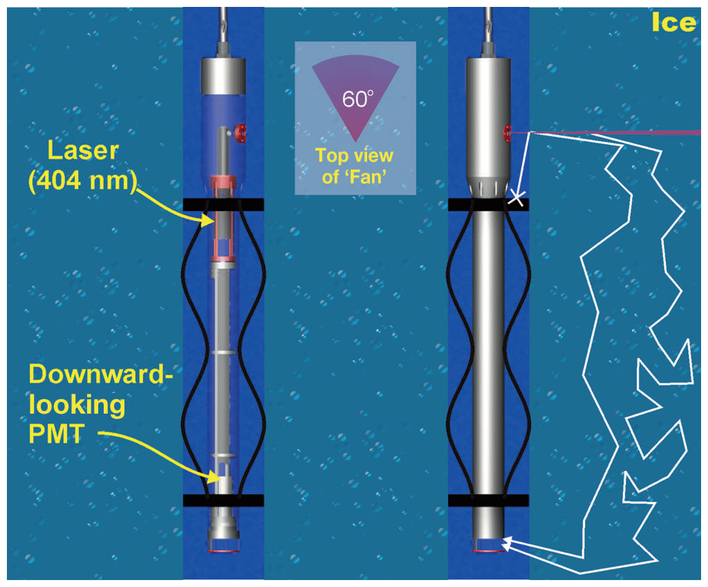
Figure 1 Sketch of the laser dust logger. Light emitted by a 404 nm diode laser in a 60^∘ horizontal fan can only reach the photon counter (PMT) below by scattering on nearby impurities.

The intensity of the light source can be adjusted throughout the logging process. To avoid stray light contamination from reflections on the hole–ice interface, multiple sets of black nylon baffles are attached to the side of the pressure housing. These also sweep ice crystals and debris out of the source beam. Spring-loaded calipers keep the logger centered in the hole.

The depth of the logger is monitored through the cable payout and onboard pressure sensors. During offline analysis, multiple logs from the same site are further aligned to achieve centimeter-scale depth precision using characteristic features such as volcanic horizons in the ice, as described by Aartsen et al. (2013).

This device has previously been deployed in West Antarctica, East Antarctica and Greenland. Due to excellent imaging properties, deployments down the water-filled boreholes (from hot water drilling and before completely refreezing after 2–3 weeks) of the IceCube Neutrino Observatory resulted in one of the highest-resolution particulate stratigraphies of any glacier available to date, as described by Aartsen et al. (2013).

To measure a potential directionality of the return signal relative to the direction of the emitted light fan, an optional extension consisting of an Applied Physics Systems Model 547 Directional Sensor (https://www.appliedphysics.com/_main_site/wp-content/uploads/model-547-micro-orientation-sensor.pdf, last access: 29 July 2020) has been fitted to the top of the logger. By measuring the local magnetic field, it deduces the absolute orientation with an azimuthal accuracy of $\pm \mathrm{1.2}{}^{\circ }$ for magnetic latitudes $<\pm \mathrm{40}{}^{\circ }$. For our application at the geographic South Pole, we estimate the azimuthal accuracy to be $\pm \mathrm{3}{}^{\circ }$.

Figure 2 Depth development of c-axis distributions (Lambert azimuthal equal-area projections) measured in SPICEcore. Depths (in meters) are indicated above each diagram. They show a clean girdle fabric below ∼1000 m. Adapted from Voigt (2017).

3 SPICEcore deployments

The South Pole Ice Core, SPC14 (see Casey et al., 2014), was drilled by the SPICEcore project in 2014–2016 at a location 2.7 km from the Amundsen–Scott station using the Intermediate Depth Drill designed and deployed by the U.S. Ice Drilling Program (IDP) (Johnson et al., 2014). It reached a final depth of 1751 m (Winski et al., 2019), surpassing the original 1500 m goal.

The core was retrieved in 2 m segments with a diameter of 98 mm. The resulting 126 mm diameter drill hole was filled with the non-freezing drilling fluid Estisol 140 and has been preserved for future logging access.

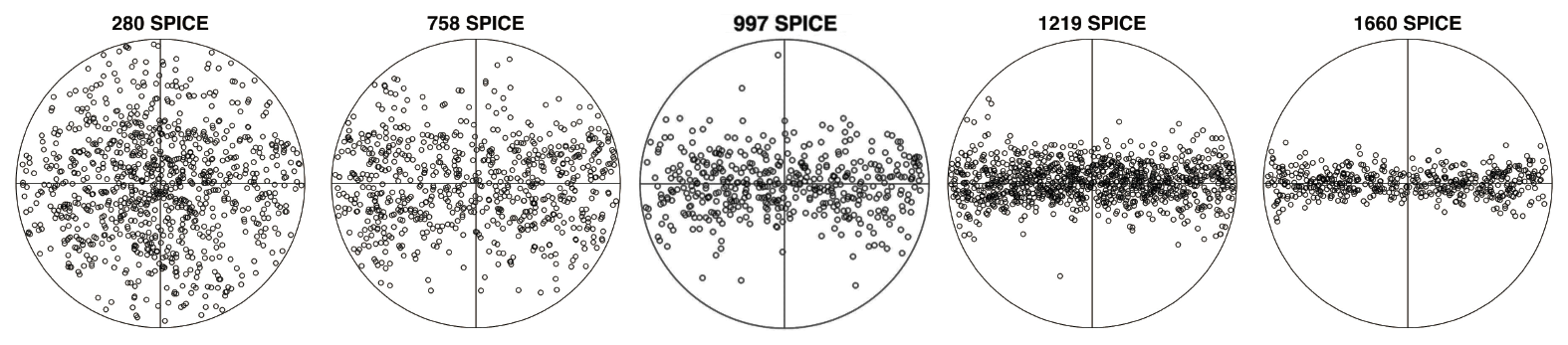
Unlike most ice coring sites, the geographic South Pole is not near an ice divide but rather on a flank site with a local flow velocity of 10 m per year. The associated accumulation site for the deepest ice is believed to be Titan Dome (Lilien et al., 2018), meaning that the ice has been transported as far as 200 km. The stress experienced below ∼800 m depth has resulted in a very prominent and continuously strengthening girdle fabric as measured by Voigt (2017). Figure 2 shows example c-axis distributions from the SPC14 ice core at various depths.

The oriented dust logger was deployed down the SPICEcore hole twice during the 2016/2017 season, both times using the Intermediate Depth Logging Winch provided by the IDP. Due to a limited available cable length, it was only able to reach a depth of 1577 m of the 1751 m cored. During the first log, the laser intensity was not yet optimized, leading to saturated and thus unusable data above 1000 m.

Two further deployments down to ∼1700 m were performed during the 2018/2019 season. Due to mechanical problems with the winch cable payout, depth readings from the winch itself are inaccurate. Only one deployment could be depth aligned to the required precision using characteristic features, as previously discussed. This deployment includes an additional round-trip between 1354 and 1703 m. Table 1 summarizes the properties of the logs used for the measurements presented here.

Table 1 Summary of usable logs obtained within the 2016/2017 and 2018/2019 logging seasons.

As shown in Fig. 3, the logger rotates as it descends and ascends the hole mainly due to the residual twist in the logging cable. On ascent, as the cable is pulling the tool up, it undergoes a smooth rotation of slightly varying angular velocity. On descent the logger sinks under its own weight and the rotation is not continuous. The most likely explanation is that the logger is repeatedly stuck on the wall before slipping.

Figure 3 Rotation of the tool descending and ascending the bore hole. A smooth and continuous rotation of slightly varying angular velocity is observed when ascending. During descent, the rotational movement is erratic. (The azimuthal orientation is with respect to local grid bearings. Grid north (0^∘) aligns with the Greenwich meridian.)

4 Anisotropy signature

The data obtained from the oriented dust logger consist of orientation, depth and optical return signal measurements at 10 ms intervals. At the usual deployment speed, this is equivalent to a sampling distance of ∼2.5 mm.

While the photomultiplier is located ∼850 mm below the laser light source, the depth resolution, as measured by Bramall et al. (2005) as the smearing of an ash layer, is dominated by the vertical extent of the laser beam and is less than a few millimeters. This allows for a continuous record of optical properties down the entire depth of a drill hole at a vertical resolution of less than a year of deposition, assuming an annual layer thickness of 1–2 cm in the deep ice as reported by Aartsen et al. (2013).

Above the transition region of air bubbles to clathrate hydrate (Miller, 1969) at 700–1300 m, the return signal is dominated by scattering on air bubbles. Below, the return signal is primarily proportional to the concentration of impurities contributing to scattering. The resulting high-resolution stratigraphy is exemplified in Fig. 4.

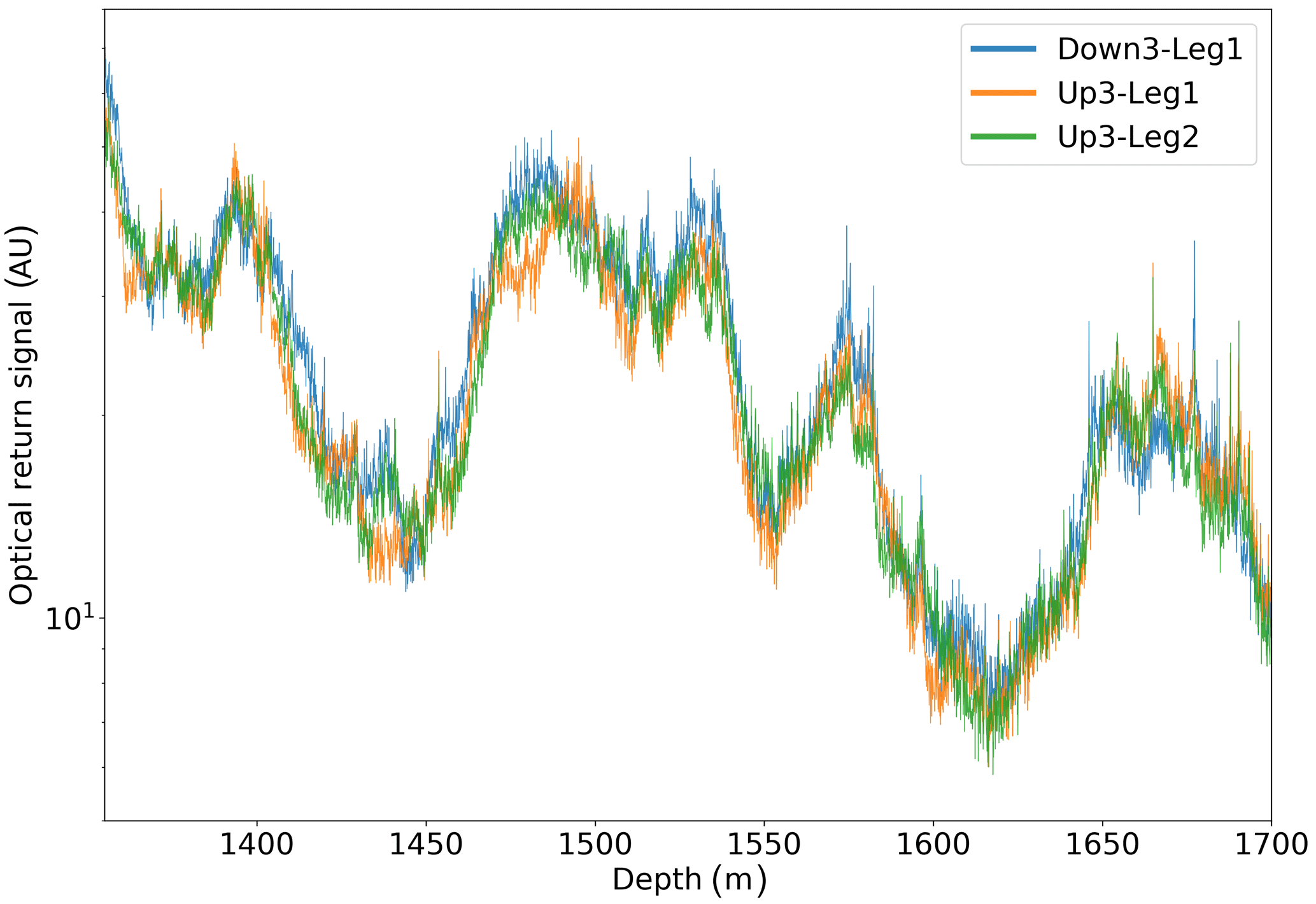
Figure 4 Example detail of optical stratigraphies obtained by logging the same depth range three times.

This figure also shows that the optical return signals at the same depths are not consistent between logs. Instead, the signal depends on the absolute orientation of the logger. We extract this anisotropy signature by taking the ratio of two logs. Usually, the ratios of raw data are on average non-unity and show slow, continuous variations. These systematic offsets, caused, for example, by the changing clarity of the drilling fluid or grime accumulation on the logger, are corrected using a second-degree polynomial fitted to the ratio.

Example ratios for ∼100 m depth slices and after fitting and correcting the offset for each depth slice are given in Fig. 5. When the device's orientation between logs is out of phase, pointing in different directions at the same depth, the ratio in these examples becomes as large as 1.5. When the logs are in phase, the observed intensities are equal and thus the ratio is unity.

Analysis of the 18/19 logging season reveals that two logs, Down3-Leg1 and Down3-Leg2, exhibit strongly correlated orientations. As exemplified in Fig. 6, the orientations of the two descending segments in the depth range between 1354 and 1703 m show nearly identical orientations, which suggests that the rotation of the tool may have been governed by the hole geometry itself. As a result, the ratio of the two logs is consistent with unity when the logs align, and the spread of 2 % standard deviation indicates the typical short-term intensity fluctuations seen in the measurement.

Figure 5 Example fits to the intensity ratio in ∼100 m depth slices. The red and black dotted lines denote the orientations of the two used logs. (The orientation is defined as the cosine of the azimuth angle.) Blue is the intensity ratio. Green is the fitted intensity ratio using Eq. (1).

In the following analysis, log Down3-Leg2 is excluded from the analysis as it is fully correlated with Down3-Leg1. The number of remaining usable ratios at each depth range available from N logs is given by the binomial coefficient $\left(\begin{array}{c}N\\ \mathrm{2}\end{array}\right)$ and varies between 3 and 21.

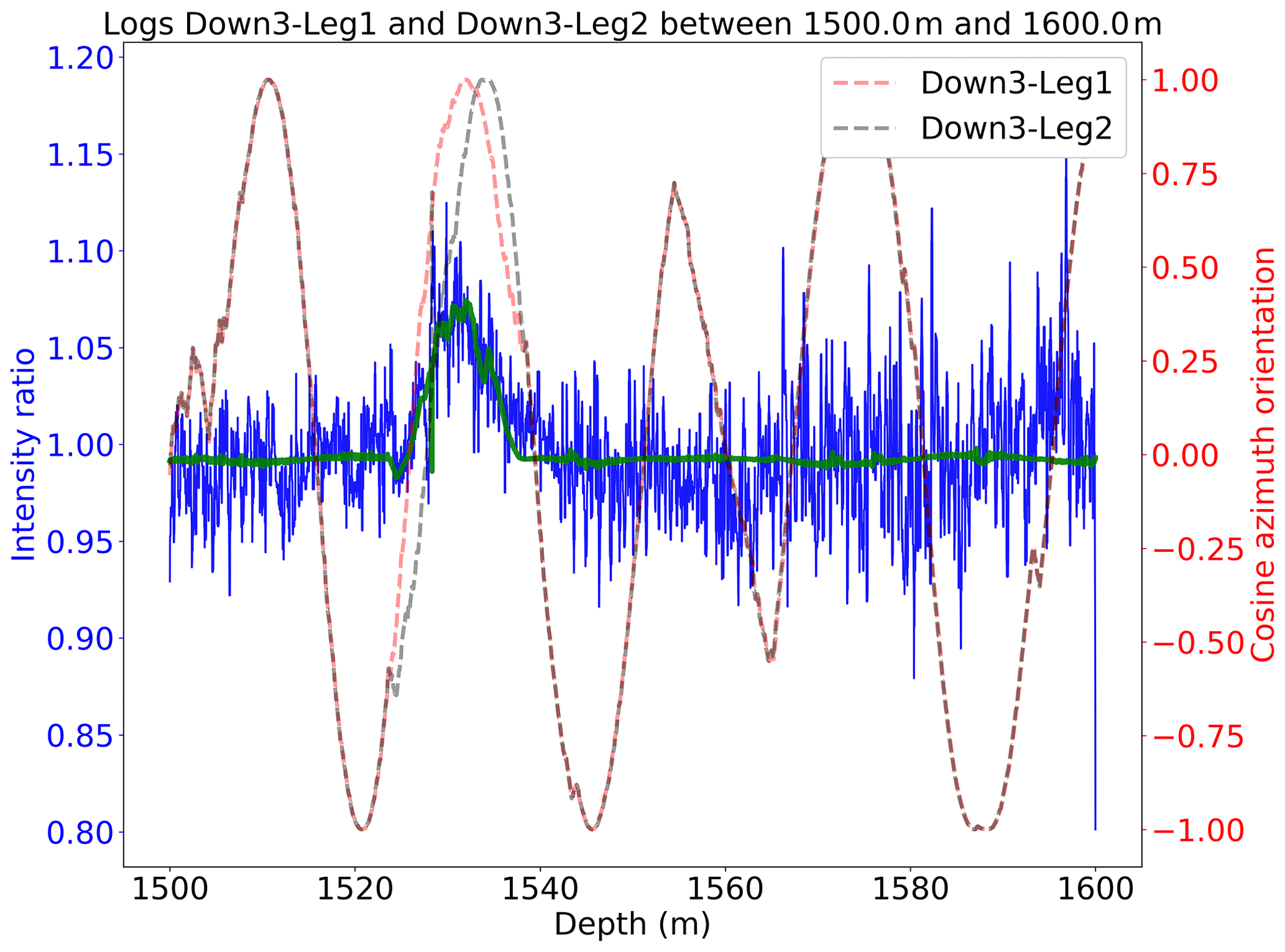
Figure 6 The intensity ratio of two log segments with near identical orientations is unity and shows the typical spread of the data.

Lacking a mature first-principle explanation and simulation of the anisotropy effect and experimental setup, the ratios have instead been found to be well-described by the following empirical relationship:

$$\begin{array}{}\text{(1)}& \text{intensity ratio}={\displaystyle \frac{\mathrm{1}+a\cdot \cos (\mathrm{2}\cdot ({\mathit{\alpha }}_{\mathrm{1}}-\mathit{\varphi }\left)\right)}{\mathrm{1}+a\cdot \cos (\mathrm{2}\cdot ({\mathit{\alpha }}_{\mathrm{2}}-\mathit{\varphi }\left)\right)}}.\end{array}$$

Here α₁ and α₂ denote the azimuthal orientations of the logger during the two logs. While ϕ denotes the azimuthal phase angle of the anisotropy effect, also called the anisotropy axis, and is limited to 0–180^∘, a is a measure of the strength of the observed effect.

The orientations and the intensity ratio are given by the dust logger data. The free parameters a and ϕ can be determined by fitting Eq. (1) to the data from a given depth range.

Note that the chosen relationship, while being very robust and easy to extract, implicitly assumes that the anisotropy causes a relative modulation to the total signal. In case the signal is additive on top of a contribution caused by Mie scattering on impurities, as would be expected from a fabric-driven birefringence scenario, the derived strength parameter a can not directly be interpreted as the strength of the underlying effect. For example, assuming an overall constant return signal from the anisotropy, the strength parameter a would be seen to increase as the overall return signal decreases as a function of depth.

5 Depth evolution

To study the depth evolution of the anisotropy signature, the data are binned into 100 m slices. While this only allows for a rather coarse depth resolution, it ensures that at least a few rotations are seen in each ratio. Otherwise the correction polynomial could bias the signal introduced by the anisotropy, and the fit would not be able to reliably determine the phase and amplitude of each log. The systematic shift introduced by the correction polynomial was further accessed by varying its degree between 1 and 3 and was found to be below the error of the mean, which is introduced below, for all depth-slices.

In the future, a finer depth resolution may experimentally be achieved by not relying on the natural rotation of the logger as it is deployed but by artificially inducing a fast rotation or by including several azimuthally offset light sources.

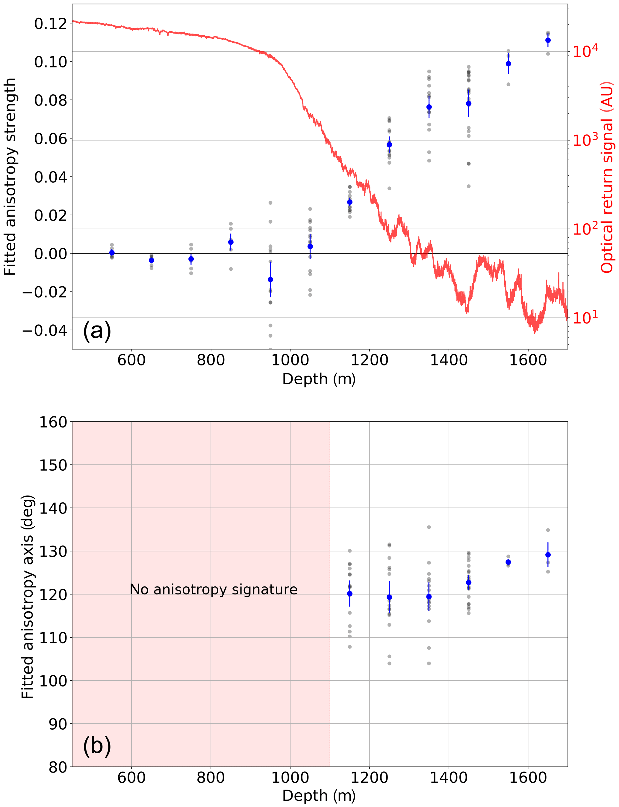
Figure 7 Depth-dependence of fitted quantities. Gray dots denote values obtained from individual ratios. The blue markers indicate the average at each depth. (a) Anisotropy strength. An example log is superimposed as reference. (b) Anisotropy axis with respect to local grid bearings. Grid north (0^∘) aligns with the Greenwich meridian.

The depth evolution of the fitted anisotropy axis ϕ and strength a as a function of depth are seen in Fig. 7. The spread of these fitted quantities between different ratios far outweighs the statistical error of the fit of each ratio. The errors on the means of each depth bin are thus constructed from the standard deviation of all ratios. While $\begin{array}{c}N\\ \mathrm{2}\end{array}$ ratios can be constructed, only N−1 are statistically independent. The error on each mean is thus given as ${\mathit{\sigma }}_{\text{mean}}=\mathit{\sigma }/\sqrt{N-\mathrm{1}}$.

Individual ratios are seen to yield consistent anisotropy axes in the deep ice. In the shallow ice above ∼1100 m where the mean strength of the observed anisotropy signal vanishes, the phase angle is unconstrained. The average axis in local grid bearings (grid north, 0^∘, aligns with the Greenwich meridian) in the deep ice is $\mathrm{126}\pm \mathrm{1}{}^{\circ }$ (statistical). Considering the 3^∘ systematic uncertainty of the orientation sensor, this direction is in good agreement with the local ice flow direction as measured by Lilien et al. (2018), as well as the optical axes of 126 and 130^∘ as fitted by Chirkin (2013) and Rongen (2019), respectively, both using IceCube data. While no anisotropy signatures are seen above 1100 m, the observed strength parameter is continuously increasing in the deeper ice. It is currently unclear what fraction of the increase in observed anisotropy strength versus depth is caused by the continuously stronger girdle fabric or by the decrease in overall scattering. However, no anisotropy signal is observed at 1000 m where the girdle fabric is already clearly developed (see Fig. 2), but bubbles still dominate the scattering at this depth. Therefore, we suspect that the anisotropy signature is smeared out to some extent due to strong local diffusion.

6 Conclusions

We have presented the first direction-dependent measurement of the intensity of backscattered, optical light in deep glacial ice. The measurement has been performed using an oriented dust logger deployed down the SPICEcore drill hole.

Below ∼1100 m, a consistent increase in received intensity is observed when the laser is aligned with the local flow axis.

This is consistent with the birefringence explanation offered by Chirkin and Rongen (2019) in which more diffusion is observed along the flow, thus leading to a higher return intensity; but this is inconsistent with the previous explanation given by Chirkin (2013) in which the effect was attributed to reduced Mie scattering along this flow. The observed sign is qualitatively also consistent with an anisotropy based on absorption.

The amplitude of the intensity modulation increases with depth. This is in part likely caused by the strengthening of the girdle fabric, as well as the strong reduction in overall scattering, as bubbles are transformed to clathrate hydrates.

To disentangle these two effects, and to potentially transition from the presented experimental ratios to a quantitative measurement of fabric properties, will require a full photon propagation simulation incorporating both Mie scattering on impurities and the diffusion introduced through the polycrystalline, birefringent fabric. While the basics for such a simulation have been outlined by Chirkin and Rongen (2019), more work will be required for the simulation to be efficient enough to be used for this application. It is currently also unclear if the intensity ratio alone will be sufficient to constrain the different fabric properties, namely the Woodcock parameters and the average grain size and shape, or if more information such as the distribution of propagation delays of individual photons may be required.