the Creative Commons Attribution 4.0 License.
the Creative Commons Attribution 4.0 License.
 | 25 Jun 2020
Measuring the location and width of the Antarctic grounding zone using CryoSat-2
Geoffrey J. Dawson
Jonathan L. Bamber
We present the results of mapping the limit of the tidal flexure (point F) and hydrostatic equilibrium (point H) of the grounding zone of Antarctic ice shelves from CryoSat-2 standard and swath elevation data. Overall we were able to map 31 % of the grounding zone of the Antarctic floating ice shelves and outlet glaciers. We obtain near-complete coverage of the Filchner–Ronne Ice Shelf. Here we manage to map areas of Support Force Glacier and the Doake Ice Rumples, which have previously only been mapped using break-in-slope methods. Over the Ross Ice Shelf, Dronning Maud Land and the Antarctic Peninsula, we obtained partial coverage, and we could not map a continuous grounding zone for the Amery Ice Shelf and the Amundsen Sea sector. Tidal amplitude and distance south (i.e. across-track spacing) are controlling factors in the quality of the coverage and performance of the approach. The location of the point F agrees well with previous observations that used differential satellite radar interferometry (DInSAR) and ICESat-1, with an average landward bias of 0.1 and 0.6 km and standard deviation of 1.1 and 1.5 km for DInSAR and ICESat measurements, respectively. We also compared the results directly with DInSAR interferograms from the Sentinel-1 satellites, acquired over the Evans Ice Stream and the Carlson Inlet (Ronne Ice Shelf), and found good agreement with the mapped points F and H. We also present the results of the spatial distribution of the grounding zone width (the distance between points F and H) and used a simple elastic beam model, along with ice thickness calculations, to calculate an effective Young modulus of ice of GPa.
- Article
(40923 KB) - Full-text XML
- BibTeX
- EndNote


In Antarctica, the majority of the grounded ice sheet (74 %, Bindschadler et al., 2011) abuts floating ice shelves or outlet glaciers. It is in this grounding zone where the ocean can directly influence the inland ice sheet. The grounding zone delineates the different stress regimes of grounded and freely floating ice. Grounded ice that was once supported by the bed is transitioning to the freely floating ice shelf and is supported partially by internal stresses and by hydrostatic pressure. The precise point at which the ice sheet detaches from the bed (i.e. the grounding line) may vary on short timescales modulated by tidal motion and bedrock slope. Ice thickness, basal drag and side drag may also vary across the grounding zone, causing rapid changes in ice velocity. Understanding ice dynamics and structure across the grounding zone is important for mass budget calculations and makes it a critical boundary for ice sheet modelling. In areas of low bedrock slope, changes in ice thickness in the grounding zone can lead to large horizontal changes in grounding line location. For example, grounding line retreat in the Amundsen Sea sector (Rignot et al., 2014; Christie et al., 2016; Scheuchl et al., 2016), caused by dynamic thinning of this part of the ice sheet (Shepherd et al., 2002; McMillan et al., 2014), has highlighted the need to monitor changes in grounding zone location as a measure of ice sheet stability.
It is not possible to measure the actual location of the grounding line with satellite remote sensing. Instead, we can study ice shelf flexure or surface geometry (such as break in slope) to infer its position. The inner limit of the tide-induced ice sheet flexure (point F) is commonly used as a proxy for the grounding line (and from here on, we will refer to this as the grounding line). Point F can be mapped using differential satellite radar interferometry (DInSAR) (Gray et al., 2002; Rignot, 1998b), repeat-track analysis of ICESat (Ice, Cloud, and land Elevation Satellite) laser altimetry (Fricker and Padman, 2006) and CryoSat-2 radar altimetry (Dawson and Bamber, 2017). We can also identify the point past which the ice shelf is in hydrostatic equilibrium (point H), providing a measure of the width of the grounding zone, W (i.e. the distance between points F and H, Fricker and Padman (2006)). However, currently DInSAR and ICESat techniques do not have sufficient spatial or temporal coverage to monitor changes across all the Antarctic grounding zone. Break-in-slope methods (Bohlander and Scambos, 2007; Bindschadler et al., 2011; Bamber and Bentley, 1994; Hogg et al., 2017) between the flat ice shelf and the grounded ice sheet also allow us to map the grounding line, but in regions where there is not a clear break in slope, this technique can be unreliable or ambiguous (Bamber and Bentley, 1994; Fricker and Padman, 2006; Brunt et al., 2010; Rignot et al., 2011; Depoorter et al., 2013). It is over these regions where ice thickness does not increase rapidly across the grounding zone that grounding line retreat is most likely, and there is good spatial and temporal coverage using DInSAR techniques. Over regions where ice thickness increases rapidly inland, and the ice sheet is not thinning, DInSAR coverage is more variable, especially in the high-latitude areas where there is limited coverage due to orbital constraints of the satellites. Using CryoSat-2 data in these areas could provide a more complete coverage of point F.
We can also use the tidal flexure of the ice sheet to investigate the structure of the grounding zone. This can help determine thickness and rheology across the grounding zone. Studies that have investigated the structure of the grounding zone through tidal flexure have, to date, mostly focused on individual ice streams. Holdsworth (1977) first used an elastic beam model as an analogue for the grounding zone. This enabled studies that used tiltmeters (Stephenson, 1984) and kinematic GPS methods (Vaughan, 1995) to measure the tidally induced deformation across the grounding zone and determine the elastic (Young's modulus) properties of the ice. More recently, DInSAR was used remotely to measure the magnitude of the tidally induced deformation across the grounding zone (Rabus and Lang, 2002; Sykes et al., 2002) and was combined with numerical elastic models (Schmeltz et al., 2002; Marsh et al., 2014) to estimate ice thickness distributions and ice properties across the grounding zone. These studies have shown that the measured Young modulus differs substantially from laboratory measurements. Fracturing in the ice can reduce its effective thickness (Hulbe et al., 2016; Rosier et al., 2017), and the elastic modulus can vary through changes in temperature and ice fabric. The ice also does not behave purely elastically over the timescales of tidal motion, and this can be investigated by treating it as a viscoelastic material (Wild et al., 2018).
The method presented here uses CryoSat-2 radar altimetry to provide a new tool that allows us to map points F and H of a significant fraction of the grounding zone. In this paper, we first present the results using 7.5 years of CryoSat-2 data to map the Antarctic grounding zone. The results are then validated against previous DInSAR and ICESat measurements. Finally, the grounding line width, W (the distance between point F and H), is then used, in combination with independent ice thickness measurements and the simple elastic beam model of the grounding zone to investigate its structure.
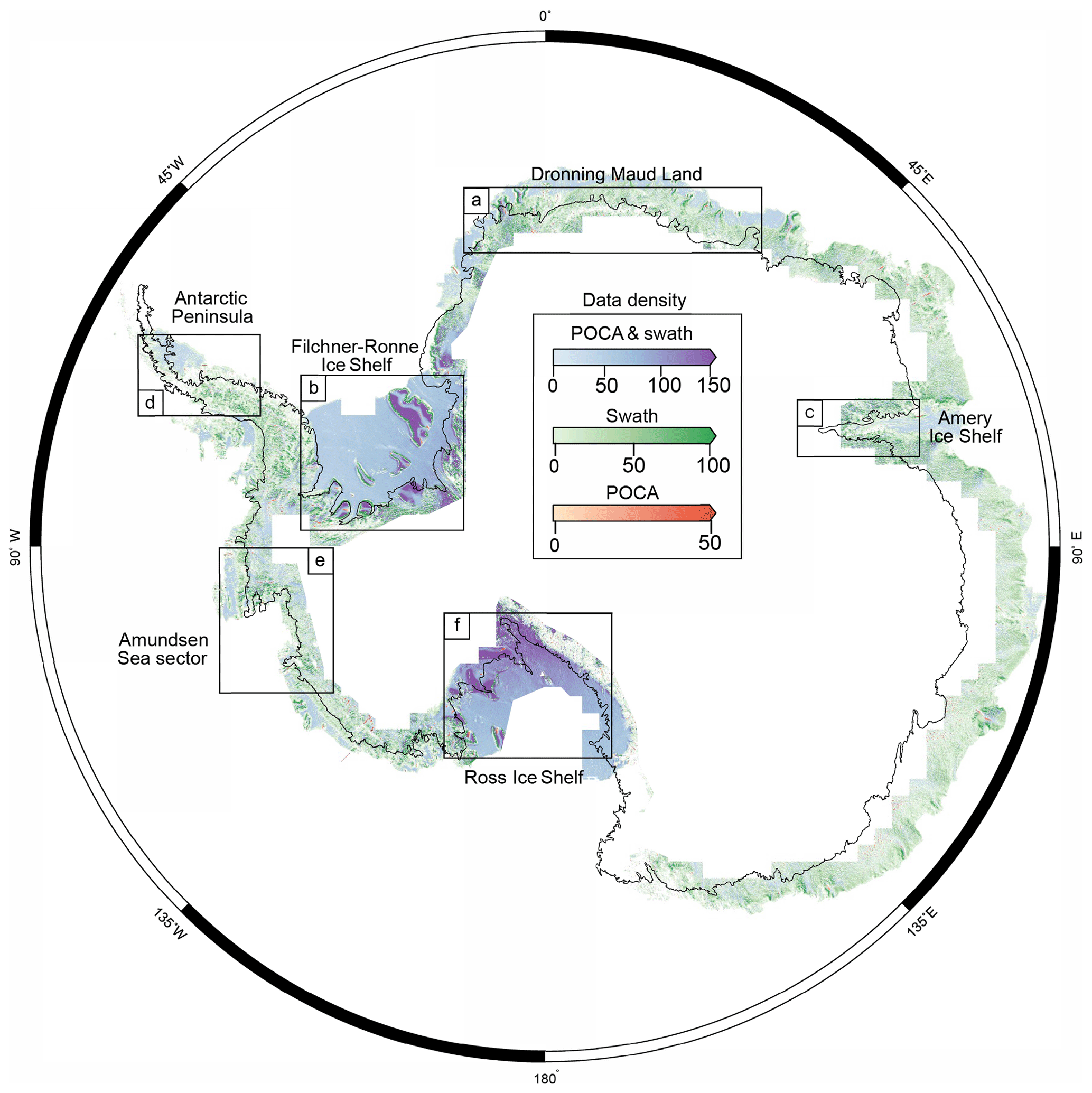
Figure 1Data coverage plot for POCA (point of closest approach) and swath data. Red, green and blue data points correspond to where we used POCA, swath or both to calculate the tidal amplitude, Td, respectively. The colour scales show the data density (POCA points per km). The swath data density is scaled by 150 (the average number of swath to POCA data points) to match the POCA density. The black line is a composite grounding line by Depoorter et al. (2013).
CryoSat-2, launched in 2010, uses a synthetic aperture radar interferometric (SARIn) mode near the margins of the ice sheet. This new mode mostly overcomes issues of off-ranging and loss of lock near breaks in slope, which have limited the coverage of conventional satellite radar altimetry over sloping terrain (Bamber et al., 2009). The SARIn mode combines delay-Doppler processing to improve along-track resolution (Raney, 1998), with dual antennas to provide the location of the return echo in the cross-track direction (Jensen, 1999). This enables the acquisition of elevation measurements based on the first return (point of closest approach or POCA) and swath-processed heights derived from the time-delayed waveform beyond the first return (Gray et al., 2013). In this study, we used CryoSat-2 POCA and swath elevation data to measure elevation change due to tidal flexure of the floating ice shelf. These data were derived from the CryoSat-2 SARIn baseline C level 1b product, with revised star tracker measurements provided by the European Space Agency (ESA). We processed POCA data using the scheme described in Helm et al. (2014) which employs a threshold re-tracker as this is less sensitive to any changes in the extinction coefficient of the snow and minimises any potential biases in elevation data. We used a processing scheme that closely follows Gray et al. (2013) to process the swath data, and we used minimum coherence and power thresholds of 0.8 and −160 db, respectively.
The coverage of POCA and swath data is shown in Figs. 1 and A1 (with a simpler plot provided in Fig. A2). POCA data provide consistent sampling over flat terrain, such as ice shelves with higher data density at high latitudes due to the narrower track spacing of the satellite. However, as they are based on the first return of the waveform, over sloping terrain, they only provide elevation measurements upslope of satellite nadir. This reduces coverage, particularly near a break in slope, such in the vicinity of the grounding line. Swath data provide elevation estimates downslope of POCA, and to obtain the best coverage of the grounding zone, we need to use a combination of POCA and swath data. While swath data tend to be noisier (Gray et al., 2017), they have an order of magnitude higher spatial sampling than POCA data. We obtain the highest sampling of swath data near breaks in slope and over moderately sloping terrain. Over the ice shelves, swath data provide improved coverage in crevassed regions; however, over the flat regions, the majority of data used is POCA. In high-sloping areas with complex topography, we generally lose coverage, for example, the Transantarctic Mountains and parts of the Antarctic Peninsula. In these regions, steep slopes can cause the satellite to lose lock, wherein the return echo of the radar wave is not captured within the range window. Also, in areas of complex topography, there may be more than one point where the radar wave reflects off the ground for a given range, leading to a loss of coherence and an ambiguous location for the located echo in the cross-track direction.
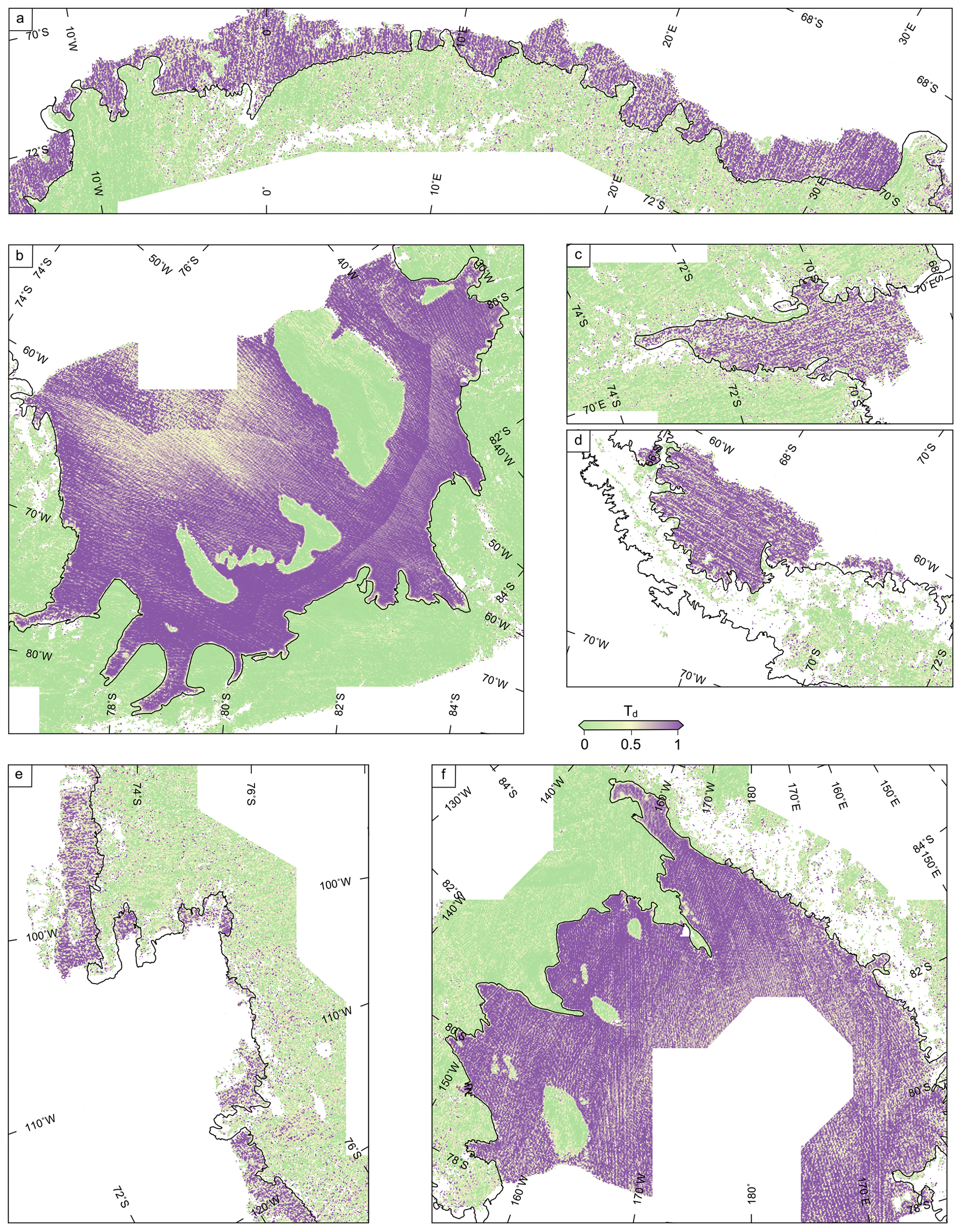
Figure 2The dimensionless tidal amplitude, Td, for (a) Dronning Maud Land, (b) Filchner–Ronne Ice Shelf, (c) Amery Ice Shelf and (d) Antarctic Peninsula. (e) Amundsen Sea sector and (f) Ross Ice Shelf. The black line is a composite grounding line by Depoorter et al. (2013).
Our approach used CryoSat-2 surface elevation measurements to determine the limit of tidal flexure of the ice (F) and the limit of hydrostatic equilibrium (H) and closely followed the technique described in Dawson and Bamber (2017). The key feature of this approach is to use the pseudo-crossover method of Wouters et al. (2015) to simultaneously solve for topography, a dimensionless tidal amplitude (Td) and, additionally in this study, a linear surface elevation rate () using Eq. (1).
where h is the elevation, t is time, a0 is the mean elevation, and a1 and a2 are the slopes of the topography in the x and y direction respectively. We used a model tidal amplitude, p (the CAT2008a tide model, which is an update to the model described by Padman et al., 2002), calculated at a constant distance of 10 km from the nominal grounding line in Depoorter et al. (2013) to scale Td. Thus, Td gives a measure of the tidal contribution to the elevation, and measures elevation change not associated with tidal motion e.g. from ice sheet thinning or changes in firn compactions rate of the floating ice. Also as we are calculating Td over a 3-year window, this method cannot capture any dynamic changes that may have occurred over this period.
We calculated Td (Fig. 2) and (Fig. A3) within a 2×2 km grid cell using CryoSat-2 data between 2010 and 2017. As we are using 7.5 years of data compared to 3 years as in our previous study, we used a 3-year moving window, weighted by a tri-cube weight function, resulting in six yearly measurements for each grid cell between 2011 and 2017. Using a 3-year moving window, we ensured that there were at least four different satellite passes per grid cell while allowing for any dynamic changes in elevation of the ice sheet that may have occurred. An alternative method would be to calculate temporal changes in Td and over the entire time series. This would require including additional parameters, which may risk overfitting the data. We then calculated the mean of Td to obtain a single value over the observation period and only used data where and , where represents the median values of the yearly measurements per cell. This removed any poor fits to Eq. (1), which likely come from erroneous elevation data. This method could potentially monitor grounding line retreat, for example, in the Amundsen Sea sector (Rignot et al., 2014; Christie et al., 2016; Scheuchl et al., 2016); however, we could not map a continuous grounding line in these areas (see Sect. 4.1). To display the reliability of this method, we have included a map of the standard deviation of Td used in calculating point F and H (Fig. A4). The lowest standard deviations are found in the high-latitude, high-tidal-range areas of the Ross Ice Shelf and the Filchner–Ronne Ice Shelf, while over the lower-latitude areas where coverage is sparser the standard deviation is high between yearly measurements.
When ice is in hydrostatic equilibrium, the real tidal amplitudes match the closest model tidal amplitudes, and we find . Over grounded ice, we find , as there is no correlation between elevation and model tidal amplitudes. Previously we mapped point F by considering ice to be influenced by the vertical motion of the tides above a certain threshold. This introduced a seaward bias, as we did not resolve amplitudes below the threshold value. In this study, we fitted an error function perpendicular to the grounding zone to determine F and H, and we removed any potential bias. This process was performed iteratively: we first mapped the centre line of the grounding zone (i.e. Td=0.5 contour) with a 1000 m spacing. We then sampled Td perpendicular to the initial guess of the centre line of the grounding zone, and fitted an error function to find a new location for Td=0.5 as well as points F (Td=0.1) and H (Td=0.9). The centre line of the grounding zone was then resampled to 1000 m spacing, and the process was repeated. The process was repeated at least three times or until the grounding line location did not change significantly by visual inspection. To make the fitting method more robust, we fixed the maximum and minimum value to 1 and 0, respectively, and weighted the fitting process around Td=0.5, using a tri-cube weight function. We only included data points where the grounding zone width was calculated between 100 and 10 000 m, and where there was continuous coverage of Td across the grounding zone. Before imposing the 10 000 m upper limit grounding line width, we verified that no mapped regions were wider than this, and we only removed poorly fitting data. We then split the grounding line when there was a break greater than 4 km and removed any segments of mapped grounding line shorter than 20 km. Finally, we applied a 10 km along-line smoothing using the polynomial approximation with the exponential kernel (PAEK) smoothing algorithm; this removed along-line noise related to incorrectly mapping points F or H but did not significantly alter their locations.
4.1 Coverage
We were able to map the grounding zone (points F and H) for 31 % of the Antarctic floating ice shelves and outlet glaciers. The percentage mapped for several key regions are shown in Table 1. In the high-latitude areas of the Ross Ice Shelf and the Filchner–Ronne Ice Shelf, we obtained near-complete coverage. In these regions, the track spacing of CryoSat-2 is as low as 0.5 km, resulting in a high spatial sampling of the grounding zone, and we only lost coverage in high-sloping regions with complex topography, for example, the Transantarctic Mountains.
At lower latitudes, further north, the coverage is variable. The spatial sampling is lower as the track spacing of the satellite varies from 2 to 3 km. In the high-sloping, low-tidal-range (0.8–1 m) Amundsen Sea sector and the Amery Ice Shelf, we could not map a continuous grounding line. There were very few POCA data near the grounding zone, and the swath data were too noisy to resolve the tidal signal. Also, over fast-flowing ice shelves such as Pine Island and Thwaites Glacier, any surface features such as ridges will move along the direction of flow. As the surface is not sampled at the same time, this will result in a spread of elevation measurements over these features, introducing noise. Using a Lagrangian framework to correct for the movement of the ice shelves is an effective way of removing this source of noise (Moholdt et al., 2014; Gourmelen et al., 2017). However, a Lagrangian framework cannot be used in this study, as it is only valid for floating ice shelves and not over grounded ice or the grounding zone.
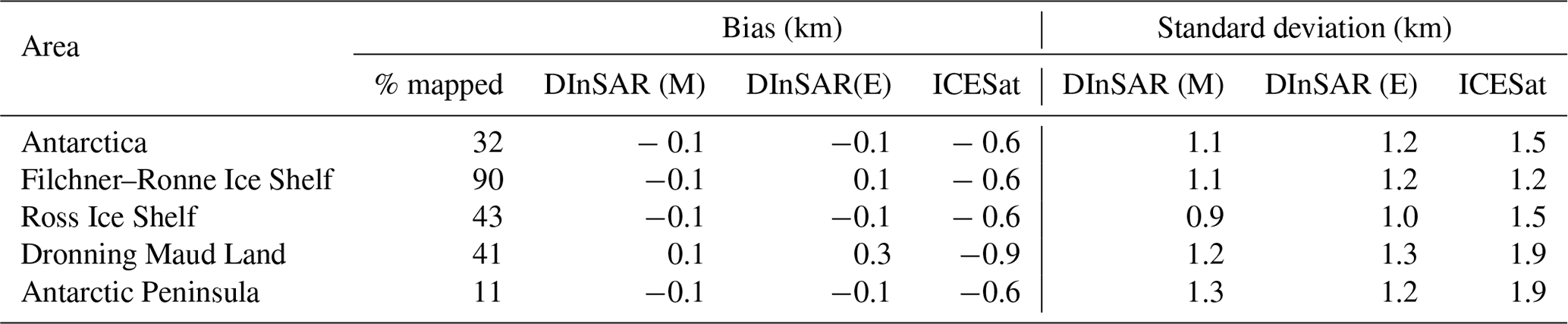
Table 1The percentage of grounding line mapped along with the bias (a negative value represents a landward bias) and standard deviation between the CryoSat-2-mapped grounding line (point F) and the DInSAR- ((M)EaSUREs and (E)SA CCI) and ICESat-mapped grounding lines, for several regions across Antarctica (shown in Fig. 1).
The coastline of Dronning Maud Land is also at relatively low latitudes. However, the tidal range is higher (1–2 m), and we were able to resolve the tidal signal using primarily swath data. We obtained 41 % coverage of the grounding zone for Dronning Maud Land. In the lower-latitude areas of the Antarctic Peninsula, the track spacing of the satellite ranges from 3 to 4 km. The spatial sampling of both POCA and swath data is lower, and we were able to map 11 % of the grounding zone. To improve the coverage in low-latitude areas we could have increased the cell size from 2 km; however, we would then not have sufficient precision to be able to compare to other methods and detect if the grounding line position has changed.
4.2 Validation with DInSAR and ICESat observations
We first compared point F mapped using CryoSat-2 to previous mapping methods that used DInSAR observations from MEaSUREs (NASA's Making Earth System Data Records for Use in Research Environments programme) and ESA Climate Change Initiative (CCI) (Rignot et al., 2016; ESA Antarctic Ice Sheets CCI, 2017) and ICESat (Brunt et al., 2010) repeat-track analysis. The absolute distance (or bias) and the standard deviation between the CryoSat-2 grounding line (defined as point F here) and the DInSAR/ICESat grounding lines for several regions are shown in Table 1. Across the whole of Antarctica, the absolute distance between the DInSAR and ICESat grounding lines and the CryoSat-2 grounding line is −0.1 km (a negative value represents a landward bias) for both datasets, showing that there is a negligible landward bias between the CryoSat-2 method and others, which does not change significantly with region. The standard deviation is 1.1 and 1.5 km between the DInSAR and ICESat grounding lines and the CryoSat-2 grounding line, respectively; however, this varies with region. In the high-latitude areas of the Ross and Filchner–Ronne ice shelves, the standard deviation is low (1.0 km between the CryoSat-2 and DInSAR grounding lines), and the grounding line matches well. While in the lower-latitude areas with large tidal range (Dronning Maud Land and Antarctic Peninsula), there is a standard deviation of 1.3 km between the CryoSat-2 and DInSAR grounding lines. This increase in standard deviation is due to reduced data density at lower latitudes, and also the smaller tidal range, which results in a noisier calculation of Td and a larger deviation from previous observations. This larger variability in mapping is also shown in the standard deviation of Td (Fig. A4), where the largest standard deviations are found over the Dronning Maud Land and Antarctic Peninsula. In comparison, the grounding line mapped using Rignot et al. (2016) has a bias of −0.3 km with a standard deviation of 0.9 km when compared to the ESA Antarctic Ice Sheets CCI (2017) grounding line and a bias of −0.4 km with a standard deviation of 1.1 km when compared to the ICESat grounding line.
We also compared our results directly with DInSAR interferograms from the Sentinel-1 satellites, acquired over the Evans Ice Stream and the Carlson Inlet (Ronne Ice Shelf). We used single look complex (SLC) synthetic aperture radar (SAR) images acquired by the Sentinel-1 satellites in the interferograms wide swath mode. The SAR operates in the C band at 5.405 GHz and, in the wide swath mode, leads to a 5×20 m resolution in ground range and azimuth. Each satellite has a repeat cycle of 12 d, and by using both Sentinel-1A and 1B, we were able to form the double-differenced interferograms from three scenes spanning between 21 July and 3 August 2018. The data were processed using GMTSAR, with the effects of topographic phase being removed using the Reference Elevation Model of Antarctica (REMA) (Howat et al., 2019). By calculating the difference between two interferograms, we removed any signal that is common to both interferograms (e.g. constant ice flow) and only measured changes in ice flow and deformation of the ice sheet. This region of the Filchner–Ronne Ice Shelf is a relatively stable area, and over the time frame of measurement, any elevation change will likely be due to tidal deformation. This results in very little measured deformation over grounded ice and a series of interference fringes that corresponds to the change in height between the two interferograms due to tides. The landward and seaward limit of these fringes can be robustly interpreted as point F and H, respectively. We also chose scenes where the tidal deformation was an average of 0.8 m. CryoSat-2 gives an average of point F and H as it samples the grounding zone over a long time, and using a deformation close to the average, we reduced any potential difference in points F and H due to tidal amplitude.
The double-difference interferogram is shown in Fig. 3, and the inner and outer limit of interference fringes which correspond to the boundaries of the grounding zone agree well with the mapped points F and H from CryoSat-2. Each fringe corresponds to approximately 2.8 cm change in height, and by unwrapping the interferogram using the snaphu method (Chen and Zebker, 2001), we were also able to compare the difference in height caused by tidal deformation. Two cross sections over the Evans Ice Stream and the Carlson Inlet are shown in Fig. 4, and by normalising the deformation, we could compare the results directly for two cross sections (the third cross section did not have any usable SAR data). In both cross sections, Td approximately matches the deformation measured by DInSAR, and points F and H match well. However, Td does not match the exact shape of the deformation. In the DInSAR data, we observe a sharp transition between fully grounded and partially grounded ice and a smoother transition to fully floating ice. This detail is not captured by CryoSat-2 as it does not have the precision to detect these small changes in elevation to resolve the tidal deformation fully.
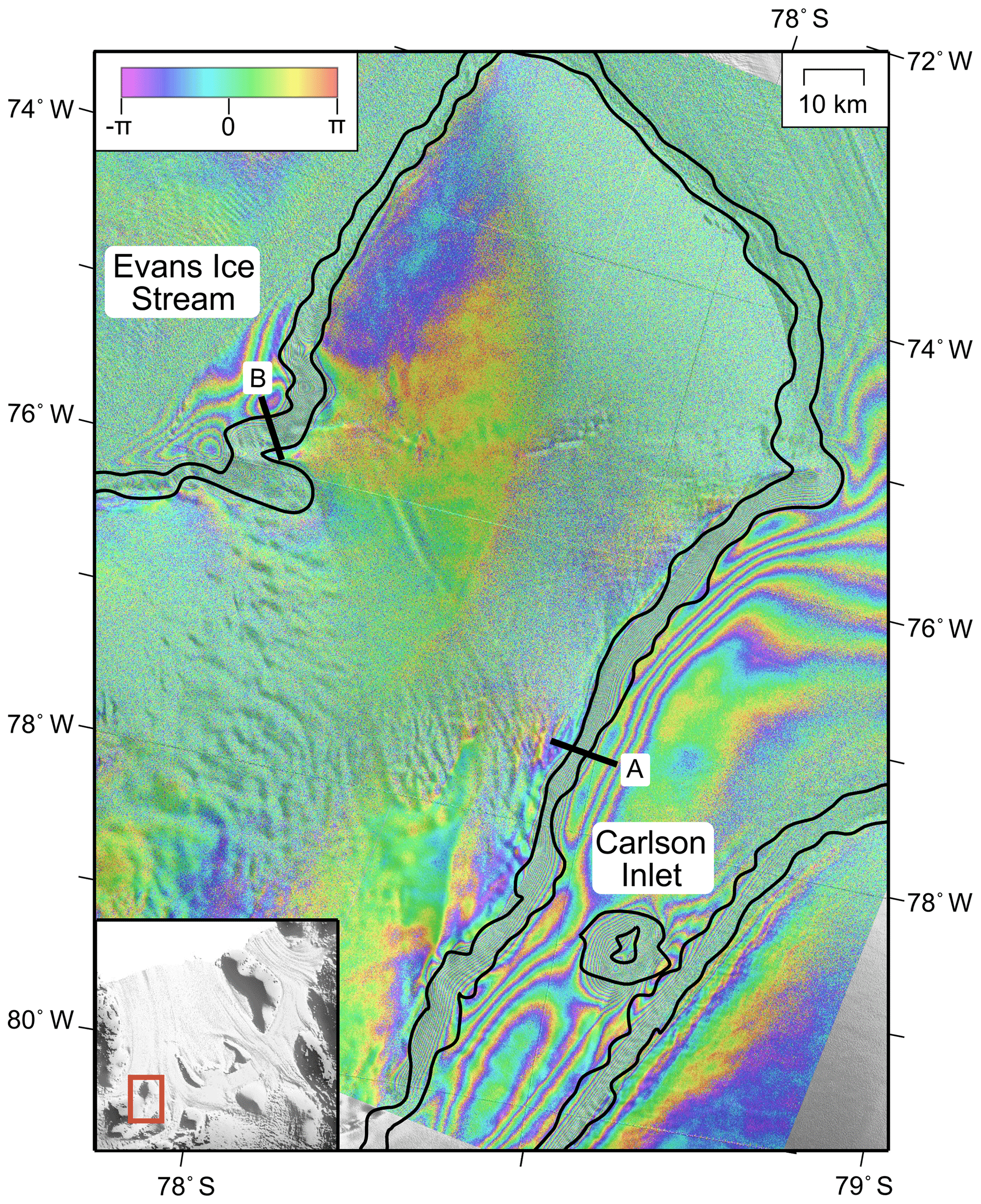
Figure 3DInSAR interference fringes over the Evans Ice Stream and the Carlson Inlet of the Filchner–Ronne Ice Shelf, along with the CryoSat-2-mapped grounding line (points F and H, solid black lines); each fringe corresponds to 2.8 cm change in height due to the motion of tides.
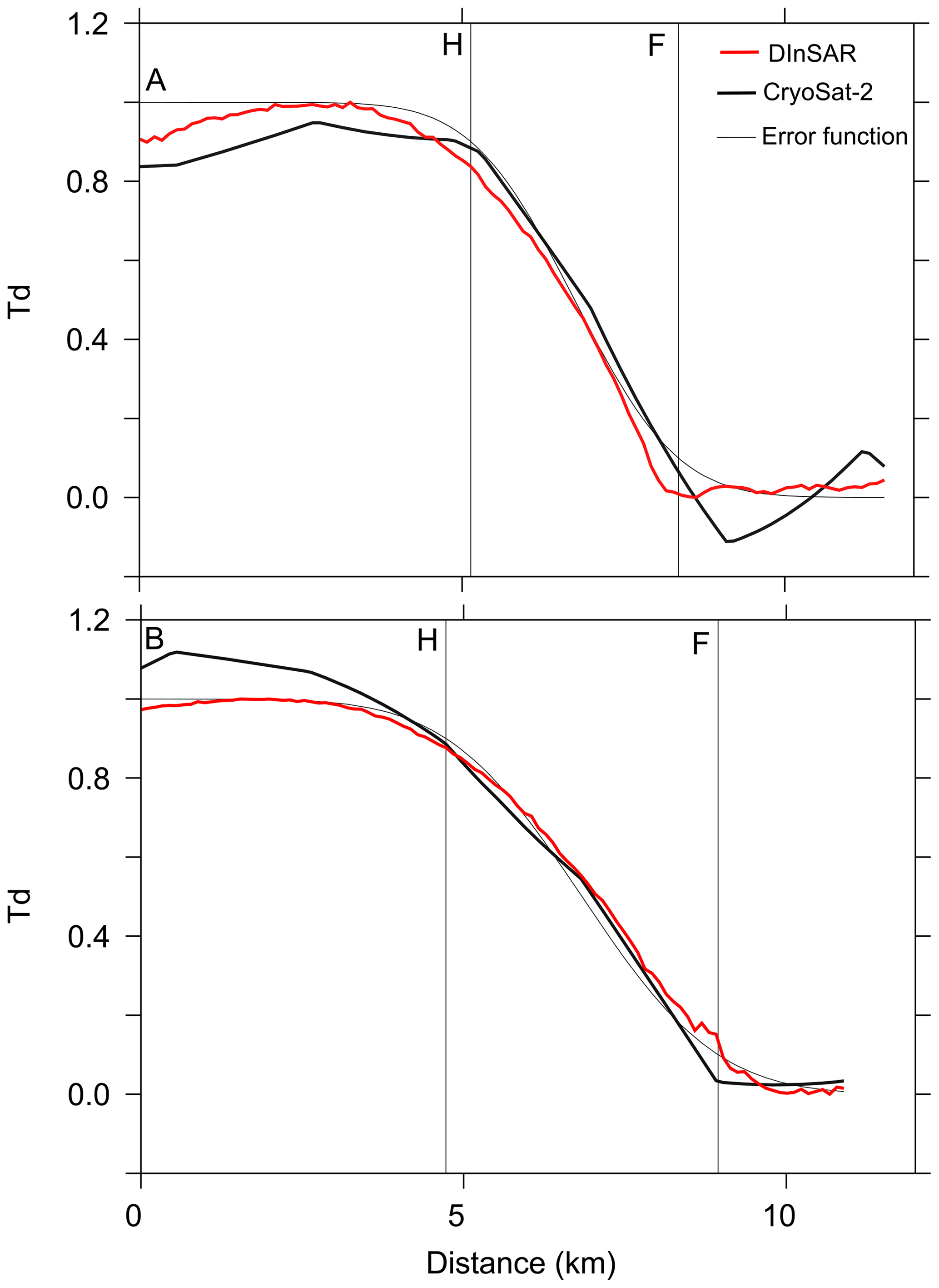
Figure 4Cross sections of Td (solid black line) with the fitted error function (dashed black line) and the normalised deformation measured from Sentinel-1 double-differenced interferograms (red line), for two cross sections across the Carlson Inlet (a) and Evans Ice Stream (b) as shown in Fig. 3.
In this paper we focus on the Filchner–Ronne Ice Shelf and the coastline of Dronning Maud Land. Over these regions and the Siple Coast region of Ross Ice Shelf, we obtained sufficient coverage of the grounding zone that allowed us to compare, and potentially add, to the existing grounding line map. The coverage over the Siple Coast region of Ross Ice Shelf was detailed in Dawson and Bamber (2017), highlighting that the grounding zone over the Echelmeyer Ice Stream was approximately 25 km inland from the previous grounding line estimate of ICESat and break-in-slope methods.
For the coastline of Dronning Maud Land, the MEaSUREs and the ESA CCI grounding line have near-complete coverage of the grounding zone (98 %), and CryoSat-2 has mapped no new locations. Over areas where there is coverage, we observe no significant deviation from the previous products. The DInSAR-mapped grounding lines were recorded between 1992 and 2014 and between 1995 and 2017 for the MEaSUREs and the ESA CCI grounding lines respectively. This indicates no observable change in the grounding line position between then and the current measurements of CryoSat-2.
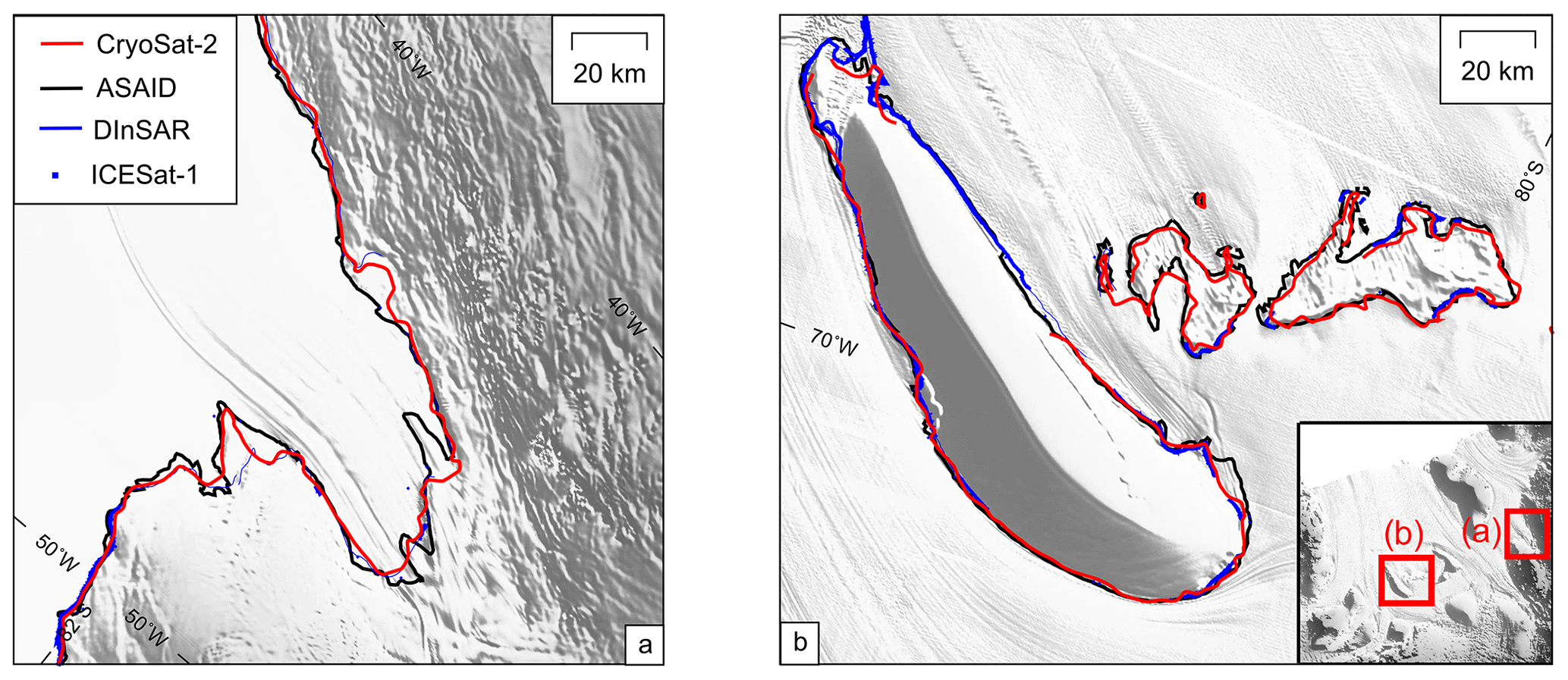
Figure 5Grounding line mapped using DInSAR from both the MEaSUREs and the ESA CCI grounding line and ICESat-1 (blue), break in slope from the ASAID project grounding line (Bindschadler et al., 2011) (black) and CryoSat-2 (red) methods for (a) Support Force Glacier and (b) Doake Ice Rumples. The background image is overlain on the REMA digital elevation model (DEM) (Howat et al., 2019).
Overall the MEaSUREs and the ESA CCI grounding lines provide 91 % and 66 % coverage of the grounding zone for the Filchner–Ronne Ice Shelf, with a combined coverage of 97 %. Over the regions where the mapped CryoSat-2 grounding zone coincided with DInSAR measurements, again, we observed no significant deviations. However, there are some areas over Support Force Glacier and the grounding zone around the Doake Ice Rumples which have not been mapped using DInSAR shown in Fig. 5. These regions have previously been mapped only using break-in-slope methods (e.g. the Antarctic Surface Accumulation and Ice Discharge (ASAID) project grounding line, Bindschadler et al., 2011), and we can see the Doake Ice Rumples where the grounding zone matches well. However, over Support Force Glacier, there are several places where point F measured by CryoSat-2 differs from the break in slope of the ice sheet of more than 10 km. These are areas where there is no clear break in slope, and the grounding line has likely been incorrectly mapped.
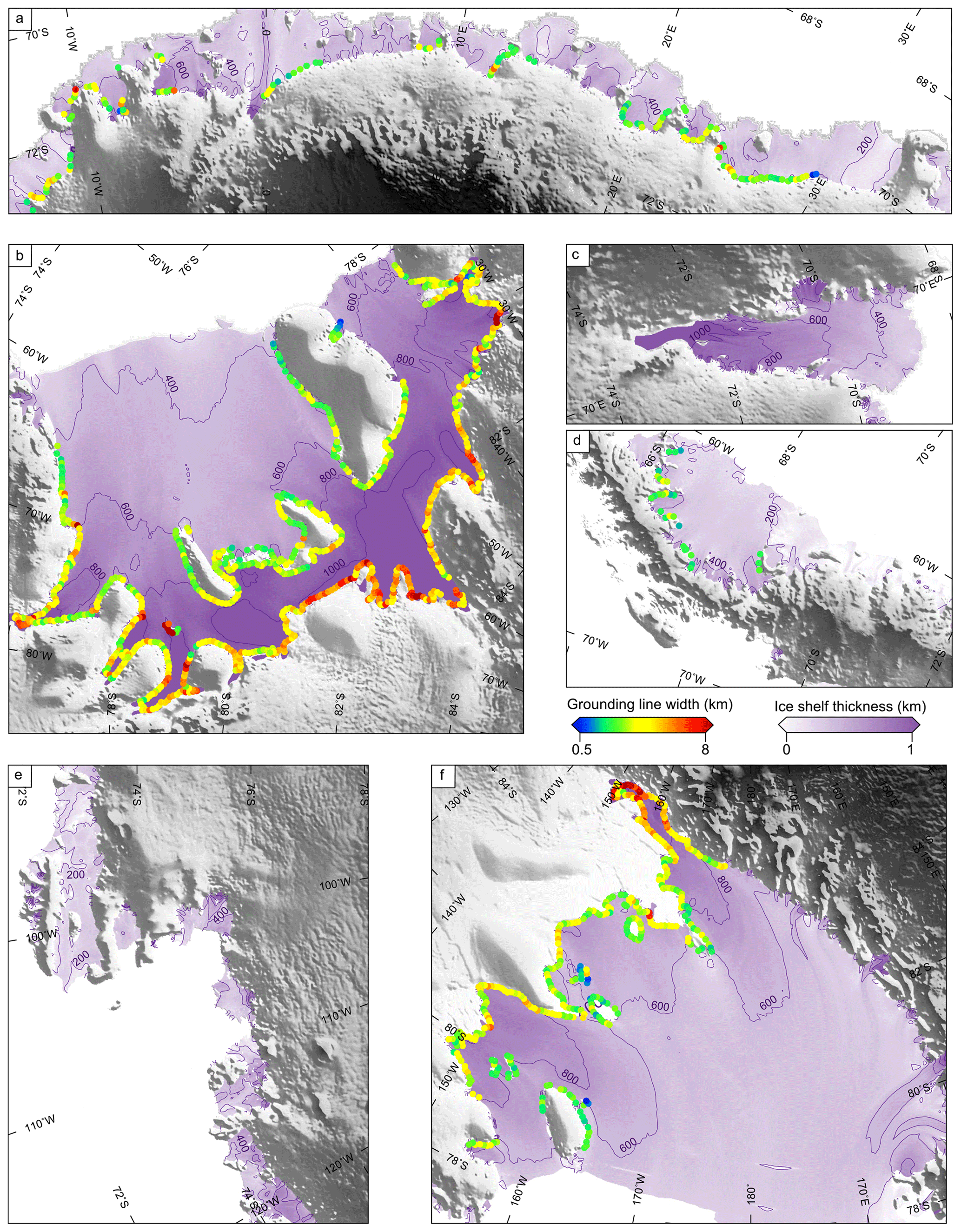
Figure 6Grounding line width (W) for (a) Dronning Maud Land, (b) Filchner–Ronne Ice Shelf, (c) Amery Ice Shelf and (d) Antarctic Peninsula. (e) Amundsen Sea sector and (f) Ross Ice Shelf. The background image is the ice shelf thickness (Chuter and Bamber, 2015) overlain on the Bedmap-2 DEM (Fretwell et al., 2006).
The width of the grounding zone (W) is shown in Fig. 6 for several regions across Antarctica and has a strong regional variation. The widest grounding zones were found over the Mercer (Ross Ice Shelf), Institute and Möller ice streams (Filchner Ice Shelf), while the narrowest regions were found over ice shelves of Dronning Maud Land. To a first approximation, this variation in grounding zone width can be attributed to the ice thickness of the grounding zone (see Fig. 5). The thicker ice tends to be more inflexible, and consequently the internal stresses of the ice can support the ice further from point F. We can demonstrate this by modelling the grounding zone as a semi-infinite beam of constant thickness (Holdsworth, 1977). With this model, the vertical deflection of the beam (w) is described by
where the beam is pinned at a hinge line at x=0, and it is displaced vertically by A0. The spatial wavenumber, β, is given by
where h is the ice thickness, E the Young modulus, ν the Poisson ratio, ρw=1026 kg m−3 the density of seawater and g the acceleration due to gravity. Given this relationship, the strongest dependence on spatial wavenumber is the thickness of the ice. Bindschadler et al. (2011) used this relationship, the elastic properties of ice (ν=0.3 and GPa) and parameters from the Rutford Ice Stream (Vaughan, 1995) to estimate the grounding line width, . If we compare W to ice shelf thickness measurements (Chuter and Bamber, 2015) at point H calculated from CryoSat-2 POCA elevation data using the assumption of hydrostatic equilibrium, we find , which agrees well with the previous relationship (Fig. 7). This also allows us to directly derive an effective Young modulus of ice as GPa, using ν=0.3.
There is considerable scatter between these results due to significant measurement errors from both h and W and because other factors such as ice rheology vary regionally. Ice shelf thickness measurements have shown to have a mean percentage error of 4.7 % near the grounding zone of the Amery Ice Shelf (compared to radio echo sounding measurements, Chuter and Bamber, 2015). These errors could be larger in some areas, for example, due to uncertainties in firn compaction in areas of compressive flow (Bamber and Bentley, 1994) and variations in damage mechanics along shear margins. These parameters may vary over areas where there are rapid changes in ice dynamics and bed topography potentially introducing larger errors. The grounding zone width is also dependent on ice rheology, the motion of the ice sheet, grounding line geometry, tidal range and grounding line migration, with these factors also contributing to the observed scatter. Other models that include 2-D flexure of the ice shelf (Schmeltz et al., 2002; Marsh et al., 2014) or modelling ice as a viscoelastic material (Wild et al., 2018) would provide a more accurate representation of the grounding zone. However, a sophisticated model is beyond the scope of the present study, and the data are too noisy to infer any further information about the structure of the grounding zone. Nevertheless, the effective Young modulus calculated here of GPa agrees well with previous calculations of GPa, E=1.1 GPa and E=9 GPa by Vaughan (1995), Smith (1991) and Stephenson (1984) respectively, while other modelling studies have found the range between E=0.8 and 3.5 GPa (Schmeltz et al., 2002) and (Marsh et al., 2014).

We used 7.5 years of CryoSat-2 SARIn POCA and swath data to map points F and H of the Antarctic grounding zone. We managed to obtain near-complete coverage of the grounding zones of the Siple Coast region of the Ross Ice Shelf and Filchner–Ronne Ice Shelf. However, in lower-latitude areas, further north, coverage is variable. Where the tidal range is small and swath data were the primary data source for resolving the tidal signal (e.g. the Amundsen Sea sector), we lose coverage, while in areas with a larger tidal range such as Dronning Maud Land and the Larsen Ice Shelf, we were able to map a significant proportion of the grounding zone. The mapped point F compared well to previous methods with a negligible bias of −0.1 and −0.1 km and a standard deviation of 1.1 and 1.5 km between DInSAR and ICESat measurements, respectively. Over these regions we observed no significant deviation between the previously mapped point F, as these regions are known to be relatively stable with no significant grounding zone retreat previously recorded, and our results support this. For the Support Force Glacier and the Doake Ice Rumples of the Filchner–Ronne Ice Shelf, we mapped regions that were previously only mapped using break-in-slope methods.
The results of mapping points F and H investigated the spatial distribution of the grounding zone width, W, across Antarctica, allowing us to examine the grounding zone structure across a significant fraction of the Antarctic coastline. W showed a strong regional variation, and to a first approximation, the grounding line width is dependent on ice thickness. Relating our results to an elastic beam model of the grounding zone and ice shelf thickness measurements, we calculated the effective Young modulus of GPa, which compares well to previous studies. However, we could not infer any further information about the structure of the grounding zone as there are measurement errors in both ice shelf thickness and grounding zone width, as well as unmodelled factors such as grounding zone shape and ice rheology.
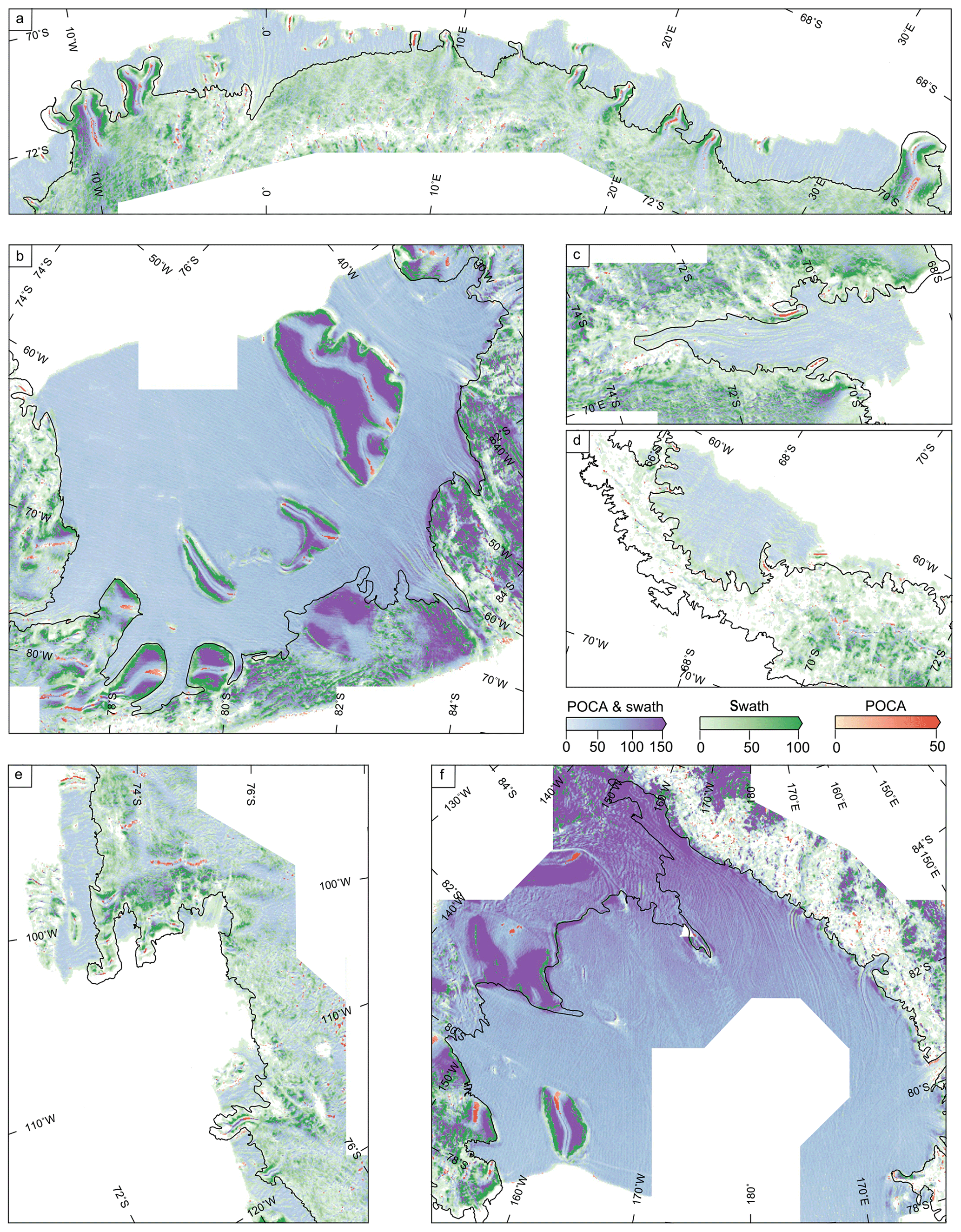
Figure A1Data coverage plot for POCA and swath data. Red, green and blue data points correspond to where we used POCA, swath or both to calculate Td, respectively. The colour scales shows the data density (POCA points per km). The swath data density is scaled by 150 (the average number of swath to POCA data points) to match the POCA density for (a) Dronning Maud Land, (b) Filchner–Ronne Ice Shelf, (c) Amery Ice Shelf and (d) Antarctic Peninsula. (e) Amundsen Sea sector and (f) Ross Ice Shelf. The black line is a composite grounding line by Depoorter et al. (2013).
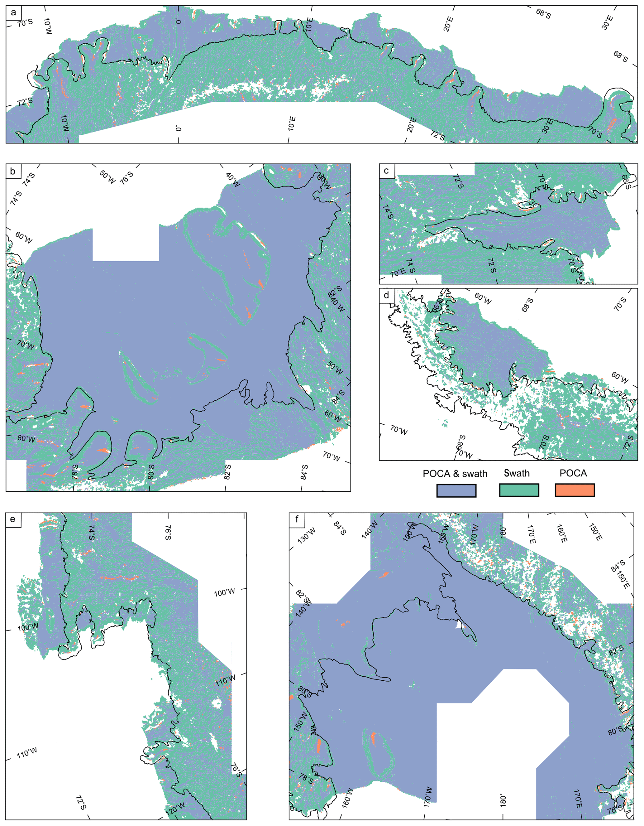
Figure A2Data coverage plot for POCA and swath data. Purple, green and orange data points correspond to where we used POCA, swath or both to calculate Td, respectively for (a) Dronning Maud Land, (b) Filchner–Ronne Ice Shelf, (c) Amery Ice Shelf and (d) Antarctic Peninsula. (e) Amundsen Sea sector and (f) Ross Ice Shelf. The black line is a composite grounding line by Depoorter et al. (2013).
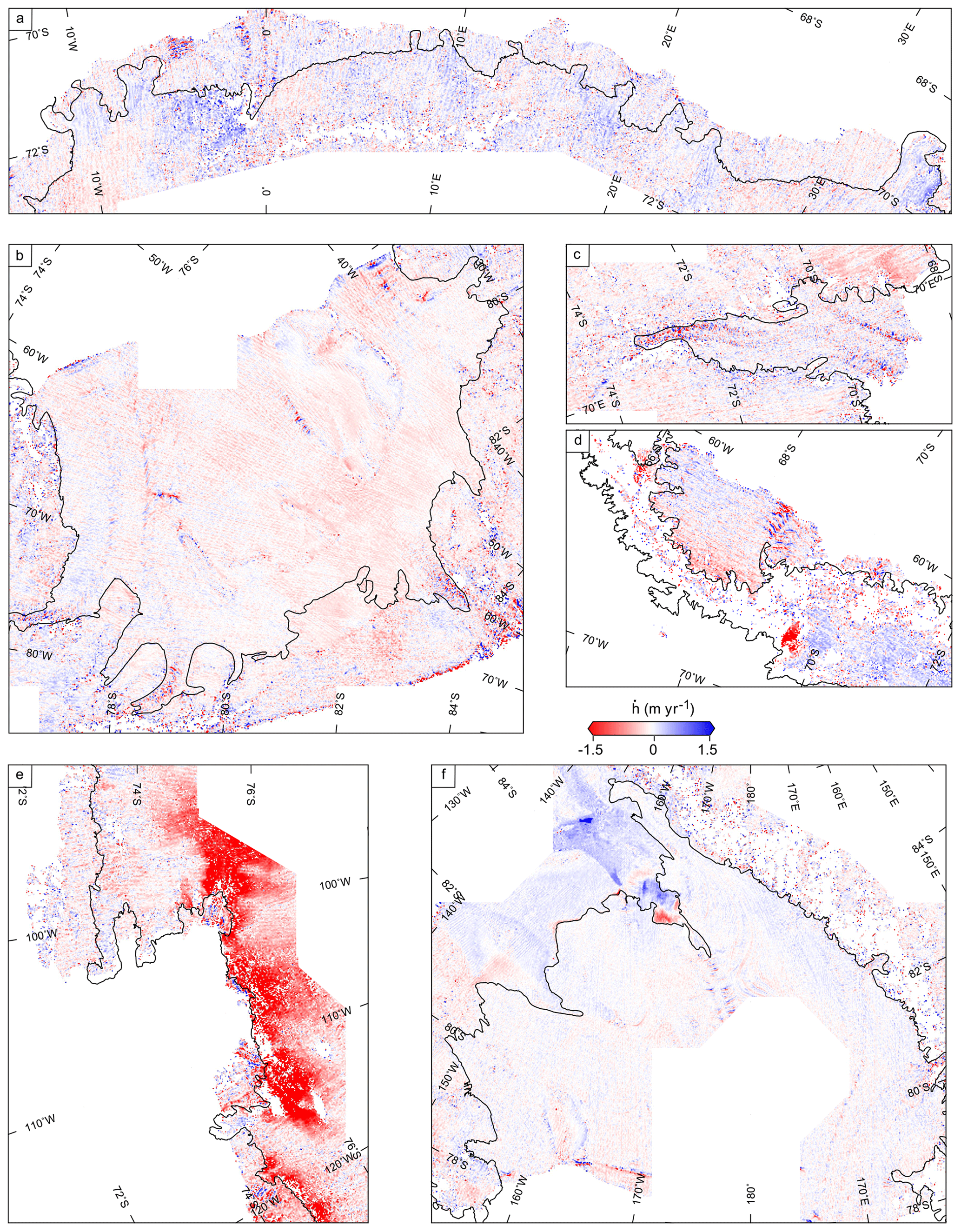
Figure A3Elevation change () for (a) Dronning Maud Land, (b) Filchner–Ronne Ice Shelf, (c) Amery Ice Shelf and (d) Antarctic Peninsula. (e) Amundsen Sea sector and (f) Ross Ice Shelf.
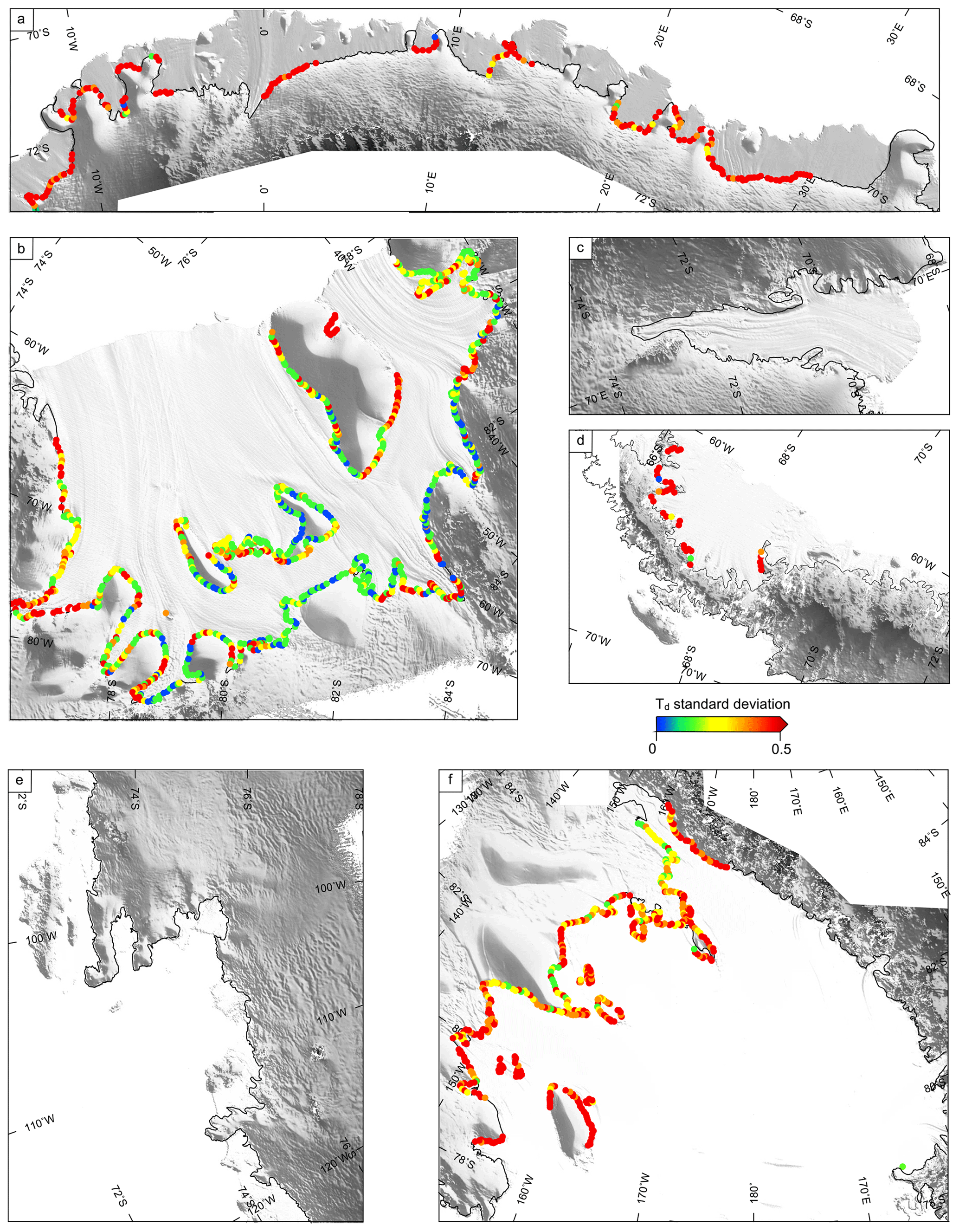
Figure A4The standard deviation of Td for the mapped grounding zone for (a) Dronning Maud Land, (b) Filchner–Ronne Ice Shelf, (c) Amery Ice Shelf and (d) Antarctic Peninsula. (e) Amundsen Sea sector and (f) Ross Ice Shelf.
The data sets generated during this study are available at https://doi.org/10.5285/40c0b0c6-533c-43e7-9761-38225dac3084 (Dawson and Bamber, 2019).
GJD undertook the data analysis, developed the methods and wrote the paper. JLB conceived the study and both authors commented on the manuscript.
The authors declare that they have no conflict of interest.
The European Space Agency (ESA) provided the CryoSat-2 data used for this research. We thank Laurence Gray for his advice in processing the CryoSat-2 swath data.
This research has been supported by the UK Natural Environment Research Council (NERC) (grant no. NE/N011511/1).
This paper was edited by Kerim Nisancioglu and reviewed by four anonymous referees.
Bamber, J. L. and Bentley, C. R.: A comparison of satellite-altimetry and ice-thickness measurements of the Ross Ice Shelf, Antarctica, Ann. Glaciol., 20, 357–364, https://doi.org/10.3189/1994AoG20-1-357-364, 1994. a, b, c
Bamber, J. L., Gomez-Dans, J. L., and Griggs, J. A.: A new 1 km digital elevation model of the Antarctic derived from combined satellite radar and laser data – Part 1: Data and methods, The Cryosphere, 3, 101–111, https://doi.org/10.5194/tc-3-101-2009, 2009. a
Bindschadler, R., Choi, H., Wichlacz, A., Bingham, R., Bohlander, J., Brunt, K., Corr, H., Drews, R., Fricker, H., Hall, M., Hindmarsh, R., Kohler, J., Padman, L., Rack, W., Rotschky, G., Urbini, S., Vornberger, P., and Young, N.: Getting around Antarctica: new high-resolution mappings of the grounded and freely-floating boundaries of the Antarctic ice sheet created for the International Polar Year, The Cryosphere, 5, 569–588, https://doi.org/10.5194/tc-5-569-2011, 2011. a, b, c, d, e
Bohlander, J., and Scambos T. A.: Antarctic coastlines and grounding line derived from MODIS Mosaic of Antarctica (MOA), National Snow and Ice Data Center, Boulder, Colorado, USA, available at: https://nsidc.org/data/NSIDC-0280/versions/1 (last access: 18 June 2020), 2007. a
Brunt, K. M., Fricker, H. A., Padman, L., Scambos, T. A., and O'Neel, S.: Mapping the grounding zone of the Ross Ice Shelf, Antarctica, using ICESat laser altimetry, Ann. Glaciol., 51, 71–79, https://doi.org/10.3189/172756410791392790, 2010a. a
Brunt, K. M., Fricker H. A., Padman L., and O'Neel S.: ICESat-Derived Grounding Zone for Antarctic Ice Shelves, Boulder, Colorado, USA, National Snow and Ice Data Center, available at: https://nsidc.org/data/NSIDC-0280/versions/1 (last access: 18 June 2020), 2010b. a
Chen, C. W. and Zebker, H. A.: Two-dimensional phase unwrapping with use of statistical models for cost functions in nonlinear optimization, J. Opt. Soc. Am. A, 18, 338–351, https://doi.org/10.1364/JOSAA.18.000338, 2001. a
Christie, F. D. W., Bingham, R. G., Gourmelen, N., Tett S. F., and Muto, A.: Four-decade record of pervasive grounding line retreat along the Bellingshausen margin of West Antarctica, Geophys. Res. Lett., 43, 5741–5749, https://doi.org/10.1002/2016GL068972, 2016. a, b
Chuter, S. J. and Bamber, J. L.: Antarctic ice shelf thickness from CryoSat-2 radar altimetry, Geophys. Res. Lett., 42, 721–729, https://doi.org/10.1002/2015GL066515, 2015. a, b, c
Dawson, G. J. and Bamber, J. L.: Antarctic Grounding Line Mapping From CryoSat-2 Radar Altimetry, Geophys. Res. Lett., 44, 11886–11893, https://doi.org/10.1002/2017GL075589, 2017. a, b, c
Dawson, G. J. and Bamber, J. L.: Grounding zone location across Antarctica form CryoSat-2 radar altimetry 2010–2017, University of Bristol, https://doi.org/10.5285/40c0b0c6-533c-43e7-9761-38225dac3084, 2019 a
Depoorter, M. A., Bamber, J. L., Griggs, J. A., Lenaerts, J. T. M., Ligtenberg, S. R. M., van den Broeke, M. R., and Moholdt G.: Calving fluxes and basal melt rates of Antarctic ice shelves, Nature, 502, 89–92, https://doi.org/10.1038/nature12567, 2013. a, b, c, d, e, f
ESA: Antarctic Ice Sheet Climate Change Initiative, Grounding Line Locations for the Ross and Byrd Glaciers, Antarctica, 2011–2017, v1.0, Centre for Environmental Data Analysis, 2017. a, b
Fretwell, P., Pritchard, H. D., Vaughan, D. G., Bamber, J. L., Barrand, N. E., Bell, R., Bianchi, C., Bingham, R. G., Blankenship, D. D., Casassa, G., Catania, G., Callens, D., Conway, H., Cook, A. J., Corr, H. F. J., Damaske, D., Damm, V., Ferraccioli, F., Forsberg, R., Fujita, S., Gim, Y., Gogineni, P., Griggs, J. A., Hindmarsh, R. C. A., Holmlund, P., Holt, J. W., Jacobel, R. W., Jenkins, A., Jokat, W., Jordan, T., King, E. C., Kohler, J., Krabill, W., Riger-Kusk, M., Langley, K. A., Leitchenkov, G., Leuschen, C., Luyendyk, B. P., Matsuoka, K., Mouginot, J., Nitsche, F. O., Nogi, Y., Nost, O. A., Popov, S. V., Rignot, E., Rippin, D. M., Rivera, A., Roberts, J., Ross, N., Siegert, M. J., Smith, A. M., Steinhage, D., Studinger, M., Sun, B., Tinto, B. K., Welch, B. C., Wilson, D., Young, D. A., Xiangbin, C., and Zirizzotti, A.: Bedmap2: improved ice bed, surface and thickness datasets for Antarctica, The Cryosphere, 7, 375–393, https://doi.org/10.5194/tc-7-375-2013, 2013. a
Fricker, H. A. and Padman, L.: Ice shelf grounding zone structure from ICESat laser altimetry, Geophys. Res. Lett., 33, L15502, https://doi.org/10.1029/2006GL026907, 2006. a, b, c
Gourmelen, N., Goldberg, D. N., Snow, K., Henley, S. F., Bingham, R. G., Kimura, S., Hogg, A. E., Shepherd, A., Mouginot, J., Lenaerts, J. T., and Ligtenberg, S. R.: Channelized melting drives thinning under a rapidly melting Antarctic ice shelf, Geophys. Res. Lett., 44, 9796–9804, https://doi.org/10.1002/2017GL074929, 2017. a
Gray, L., Short, N., Bindschadler, R., Joughin, I., Padman, L., Vornberger, P., and Khananian, A.: RADARSAT interferometry for Antarctic grounding-zone mapping, Ann. Glaciol., 34, 269–276, https://doi.org/10.3189/172756402781817879, 2002. a
Gray, L., Burgess, D., Copland, L., Cullen, R., Galin, N., Hawley, R., and Helm, V.: Interferometric swath processing of Cryosat data for glacial ice topography, The Cryosphere, 7, 1857–1867, https://doi.org/10.5194/tc-7-1857-2013, 2013. a, b
Gray, L., Burgess, D., Copland, L., Dunse, T., Langley, K., and Moholdt, G.: A revised calibration of the interferometric mode of the CryoSat-2 radar altimeter improves ice height and height change measurements in western Greenland, The Cryosphere, 11, 1041–1058, https://doi.org/10.5194/tc-11-1041-2017, 2017. a
Helm, V., Humbert, A., and Miller, H.: Elevation and elevation change of Greenland and Antarctica derived from CryoSat-2, The Cryosphere, 8, 1539–1559, https://doi.org/10.5194/tc-8-1539-2014, 2014. a
Hogg, A. E., Shepherd, A., Gilbert, L., Muir, A., and Drinkwater, M. R.: Mapping ice sheet grounding lines with CryoSat-2, Adv. Space Res., 62, 1191–1202, https://doi.org/10.1016/j.asr.2017.03.008, 2017. a
Holdsworth, G.: Tidal interaction with ice shelves, Ann. Geophys., 33, 133–146, 1977. a, b
Howat, I. M., Porter, C., Smith, B. E., Noh, M.-J., and Morin, P.: The Reference Elevation Model of Antarctica, The Cryosphere, 13, 665–674, https://doi.org/10.5194/tc-13-665-2019, 2019. a, b
Hulbe, C. L., Klinger, M., Masterson, M., Catania, G., Cruikshank, K., and Bugni, A.: Tidal bending and strand cracks at the Kamb Ice Stream grounding line, West Antarctica, J. Glaciol., 235, 816–824, https://doi.org/10.1017/jog.2016.74, 2016. a
Jensen, J. R.: Angle measurement with a phase monopulse radar altimete, IEEE T. Antenn. Propag., 47, 715–724, https://doi.org/10.1109/8.768812, 1999. a
Marsh, O. J., Rack, W., Golledge, N. R., Lawson, W., and Floricioiu, D.: Grounding-zone ice thickness from InSAR: Inverse modelling of tidal elastic bending, J. Glaciol., 60, 526–536, https://doi.org/10.3189/2014JoG13J033, 2014. a, b, c
McMillan, M., Shepherd, A., Sundal, A., Briggs, K., Muir, A., Ridout, A., Hogg, A., and Wingham, D.: Increased ice losses from Antarctica detected by CryoSat-2, Geophys. Res. Lett., 41, 3899–3905, https://doi.org/10.1002/2014GL060111, 2014. a
Moholdt, G., Padman, L., and Fricker, H. A.: Basal mass budget of Ross and Filchner-Ronne ice shelves, Antarctica, derived from Lagrangian analysis of ICESat altimetry, J. Geophys. Res.-Earth Surf., 119, 2361–2380, https://doi.org/10.1002/2014JF003171, 2014. a
Padman, L., Fricker, H. A., Coleman, R., Howard, S., and Erofeeva, L.: A new tide model for the Antarctic ice shelves and seas, Ann. Glaciol., 34, 247–254, https://doi.org/10.3189/172756402781817752, 2002. a
Rabus, B. T. and Lang, O.: On the representation of ice-shelf grounding zones in SAR interferograms, J. Glaciol., 48, 345–356, https://doi.org/10.3189/172756502781831197, 2002. a
Raney, R. K.: The delay/Doppler radar altimeter, IEEE T. Geosci. Remote, 36, 1578–1588, https://doi.org/10.1109/36.718861, 1998. a
Rignot, E.: Hinge-line migration of Petermann Gletscher, north Greenland, detected using satellite-radar interferometry, J. Glaciol., 44, 469–476, https://doi.org/10.3189/S0022143000001994, 1998. a
Rignot, E., Mouginot, J., and Scheuchl, B.: MEaSUREs InSAR-based Antarctica ice velocity map, Boulder, CO, USA, NASA DAAC at the National Snow and Ice Data Center, 2011
Rignot, E., Mouginot, J., and Scheuchl, B.: Antarctic grounding line mapping from differential satellite radar interferometry, Geophys. Res. Lett., 38, L10504, https://doi.org/10.1029/2011GL047109, 2011. a
Rignot, E., Mouginot, J., Morlighem, M., Seroussi, H., and Scheuchl, B.: Widespread, rapid grounding line retreat of Pine Island, Thwaites, Smith, and Kohler glaciers, West Antarctica, from 1992 to 2011, Geophys. Res. Lett., 41, 3502–3509, https://doi.org/10.1002/2014GL060140, 2014. a, b
Rignot, E., Mouginot, J., and Scheuchl, B.: MEaSUREs Antarctic Grounding Line from Differential Satellite Radar Interferometry, Version 2, Boulder, Colorado, USA, NASA National Snow and Ice Data Center Distributed Active Archive Center, available at: https://nsidc.org/data/NSIDC-0498/versions/2, last access: 4 September 2016. a, b
Rosier, S. H. R., Marsh, O. J., Rack, W., Gudmundsson, G. H., Wild, C. T., and Ryan, M.: On the interpretation of ice-shelf flexure measurements, J. Glaciol., 241, 783–791, https://doi.org/10.1017/jog.2017.44, 2017. a
Scheuchl, B. J., Mouginot, J., Rignot, E., Morlighem, M., and Khazendar, A.: Grounding line retreat of Pope, Smith, and Kohler Glaciers, West Antarctica, measured with Sentinel-1a radar interferometry data, Geophys. Res. Lett., 43, 8572–8579, https://doi.org/10.1002/2016GL069287, 2016. a, b
Shepherd, A., Wingham, D. J., and Mansley, J. A. D.: Inland thinning of the Amundsen Sea Sector, West Antarctica, Geophys. Res. Lett., 29, 2-1–2-4, https://doi.org/10.1029/2001GL014183, 2002. a
Schmeltz, M., Rignot E., and Douglas, M.: Tidal flexure along ice-sheet margins: comparison of InSAR with an elastic-plate model, Ann. Glaciol., 34, 202–208, https://doi.org/10.3189/172756402781818049, 2002. a, b, c
Smith, A.: The use of tiltmeters to study the dynamics of Antarctic ice-shelf grounding lines, J. Glaciol., 37, 51–58, https://doi.org/10.3189/S0022143000042799, 1991. a
Stephenson, S. N.: Glacier Flexure and the Position of Grounding Lines: Measurements By Tiltmeter on Rutford Ice Stream, Antarctica, Ann. Glaciol., 5, 165–169, https://doi.org/10.3189/1984AoG5-1-165-169, 1984. a, b
Sykes, H. J., Murray, T., and Luckman, A.: The location of the grounding zone of Evans Ice Stream, Antarctica, investigated using SAR interferometry and modelling, Ann. Glaciol., 50, 35–40, https://doi.org/10.3189/172756409789624292, 2009. a
Vaughan, D.: Tidal flexure at ice shelf margins, J. Geophys. Res., 100, 6213–6224, https://doi.org/10.1029/94JB02467, 1995. a, b, c, d
Wang, F., Bamber, J. L., and Cheng, X.: Accuracy and performance of CryoSat-2 SARIn mode data over Antarctica, IEEE Geosci. Remote Sens. Lett., 12, 1516–1520, https://doi.org/10.1109/LGRS.2015.2411434, 2015.
Wild, C. T., Marsh, O. J., and Rack, W.: Unraveling InSAR Observed Antarctic Ice-Shelf Flexure Using 2-D Elastic and Viscoelastic Modeling, Front. Earth Sci., 6, 28, https://doi.org/10.3389/feart.2018.00028, 2018. a, b
Wouters, B., Martin-Español, A., Helm, V., Flament, T., van Wessem, J. M., Ligtenberg, S. R. M., van den Broeke, M. R, and Bamber, J. L.: Dynamic thinning of glaciers on the Southern Antarctic Peninsula, Science, 348, 899–903, 10.1126/science.aaa5727, 2015 a