Improved GNSS-R bi-static altimetry and independent digital elevation models of Greenland and Antarctica from TechDemoSat-1

Improved digital elevation models (DEMs) of the Antarctic and Greenland ice sheets are presented, which have been derived from Global Navigation Satellite Systems-Reflectometry (GNSS-R). This builds on a previous study (Cartwright et al., 2018) using GNSS-R to derive an Antarctic DEM but uses improved processing and an additional 13 months of measurements, totalling 46 months of data from the UK TechDemoSat-1 satellite. A median bias of under 10 m and root-mean-square errors (RMSEs) of under 53 m for the Antarctic and 166 m for Greenland are obtained, as compared to existing DEMs. The results represent, compared to the earlier study, a halving of the median bias to 9 m, an improvement in coverage of 18 %, and a 4 times higher spatial resolution (now gridded at 25 km). In addition, these are the first published satellite altimetry measurements of the region surrounding the South Pole. Comparisons south of 88^∘ S yield RMSEs of less than 33 m when compared to NASA's Operation IceBridge measurements. Differences between DEMs are explored, the limitations of the technique are noted, and the future potential of GNSS-R for glacial ice studies is discussed.

1 Introduction

The use of reflected L-band signals from Global Navigation Satellite Systems (GNSS) for Earth observational purposes was first proposed in 1988 (Hall and Cordey, 1988). GNSS-Reflectometry (GNSS-R) is now applied to the characterization of the Earth's surface predominately for the monitoring of ocean surface winds (Clarizia and Ruf, 2016; Foti et al., 2015; Foti et al., 2017; Ruf and Balasubramaniam, 2018). It has been investigated for other applications, such as altimetry of the ice sheets and oceans (e.g. Cardellach et al., 2004; Cartwright et al., 2010; Clarizia et al., 2016), soil moisture (Chew et al., 2016), and monitoring of the cryosphere (e.g. Belmonte Rivas et al., 2010; Cartwright et al., 2019; Fabra et al., 2012). GNSS-R has been found to be effective when applied to the cryosphere not only for sea ice detection (Alonso-Arroyo et al., 2017; Cartwright et al., 2019; Yan and Huang, 2016) and characterization (Rodriguez-Alvarez et al., 2019) but also for sea ice altimetry (Hu et al., 2017; Li et al., 2017) and glacial ice altimetry (Cartwright et al., 2018; Rius et al., 2017).

The application of GNSS-R to altimetry was originally proposed by Martin-Neira (1993) and has been successfully demonstrated from fixed, airborne, and spaceborne platforms. Due to the highly specular nature of reflections from ice-covered surfaces, it is a natural step to apply these techniques to the cryosphere. In these cases, spaceborne platforms have been able to achieve root-mean-square errors (RMSEs) of below 5 m when applied to limited tracks using the group delay (Hu et al., 2017) and below 5 cm where phase delay is available (Li et al., 2017). As more GNSS-R data have become available from the low Earth orbiter TechDemoSat-1 (TDS-1), it has been possible to use a larger collection of reflections for the construction of Digital Elevation Models (DEMs) of the larger ice sheets, such as Antarctica (Cartwright et al., 2018). The use of GNSS-R offers a unique opportunity to measure the elevation of ice over the South Pole due to the wide variety of incidence angles available through bi-static altimetry enabling this technique to be unrestricted by the orbital constraints of traditional monostatic radar altimetry.

The use of signals of opportunity results in GNSS-R requiring only very low-mass, low-power receiver-only systems and is therefore a low-cost method of remote sensing. The approach therefore lends itself to applications in constellation missions in order to increase spatial and temporal resolutions. Cyclone GNSS (CYGNSS) was launched in 2016 by NASA for the monitoring of winds inside tropical cyclones and has an average revisit time of 4 h (Ruf et al., 2013); however, the low inclination of these satellites (35^∘) means that their data have little application to the cryosphere. A system similar to that of CYGNSS, but optimized for cryosphere applications, has been proposed (Cardellach et al., 2018). Currently available spaceborne data over the poles is limited to that of satellite TDS-1, which was placed in a high-inclination orbit (98.4^∘) and active for a total of 46 months between November 2014 and December 2018. It is these data upon which this study is based.

As stated by Slater et al. (2018), DEMs can help in the understanding of ice sheet hydrology through mass balance calculations, grounding line thickness, and delineation of drainage basins. These further improve understanding of ice dynamics and potential sea level rise associated with ice sheets. This paper builds upon earlier work done by Cartwright et al. (2018), using an algorithm developed by Clarizia et al. (2016) for the estimation of sea surface height. Here we use improved re-tracking combined with expansion of the GNSS-R dataset and enhanced processing to yield higher accuracies over the Antarctic ice sheet. This is then applied to the Greenland ice sheet, demonstrating the flexibility of the technique and potential for high-resolution observations over these areas. These new DEMs are primarily compared with two high-resolution DEMs, exclusively from CryoSat-2 in the case of the Antarctic ice sheet (Slater et al., 2018) and from the European Space Agency Climate Change Initiative's (ESA CCI) composite of CryoSat-2 (Simonsen and Sørensen, 2017) and ArcticDEM (https://www.pgc.umn.edu/data/arcticdem, last access: 9 June 2020) in the case of Greenland. Brief comparisons are given to two additional DEMs for each ice sheet: those by Howat et al. (2014) and Bamber (2001) over Greenland and the Bedmap2 Elevation Data (Fretwell et al., 2013) and Bamber et al. (2009) over Antarctica. Further comparisons are performed over the area south of 88^∘ using the Operation IceBridge elevation dataset.

Cartwright et al. (2018) found this approach gave consistent DEM overestimations in data at higher incidence angles, therefore high incidence angle data ($>\mathrm{55}{}^{\circ }$) were discarded. In this study, we remove the incidence angle filter to increase the sample size and add an intermediate processing step, a spatial mean of all points within a certain radius of the point in question. This accounts for the overestimations of the higher incidence angle data, leading to an overall reduction in error and increase in resolution due to the larger dataset.

This paper will first describe the dataset used and the satellite platform TDS-1 in Sect. 2. Then Sect. 3 will detail the improved methods for height estimation and application over both Antarctica and Greenland. Comparison of the new DEMs against the CryoSat-2 and ESA CCI DEMs are reported in Sect. 4, along with investigations into the areas in which they differ, possible causes of these differences and brief comparisons with other DEMs. Section 5 details the benefits and limitations of this technique. Finally, Sect. 6 concludes the study.

2 TechDemoSat-1 and datasets used

TDS-1 was launched in 2014 as a technology demonstration platform by Surrey Satellite Technology Ltd. into a quasi sun-synchronous orbit of 98.4^∘ inclination at an altitude of 635 km. TDS-1 carried eight experimental payloads, one of which was the Space GNSS Receiver Remote Sensing Instrument (SGR-ReSI). It is this sensor from which the data used in this study were acquired. SGR-ReSI is extremely low mass and low power and constructed from commercial off-the-shelf components. Full details of the SGR-ReSI can be found in Jales and Unwin (2015). Due to the use of the shared platform in the demonstration operation period (November 2014–July 2017), the SGR-ReSI was only active 2 d in every 8 d cycle, whereas it was operating 24 h d⁻¹ in the final phase of the mission (August 2017–December 2018). The instrument could receive up to four GPS (Global Positioning System) reflections at any one time. This, combined with the asynchronism of the cycle of TDS-1 with that of the GPS satellites, creates a varying web of specular points over time, increasing the spatial coverage, as well as providing data over the poles, which has thus far not been possible with standard satellite altimetry due to orbital constraints.

Data from TDS-1 are provided as delay–Doppler maps (DDMs), which are maps of the scattered power in the delay and Doppler domains. A smooth reflecting surface results in a strong, coherent signal due to the majority of the power originating from the specular point, with a relatively small glistening zone (Zavorotny and Voronovich, 2000). Such DDMs have a distinct peak in power and very little spreading of the power in the delay or Doppler domain. This is in contrast to rougher reflections (for example, over the ocean surface) where a pronounced horseshoe shape is visible due to the spread of the signal in both delay and Doppler caused by signal scatter both in front and behind the specular point. At the wavelength of the GPS signals used (L1 band, ∼19 cm), ice is much smoother than the ocean surface. The strength of this return from ice is ideal for the extraction of height information. DDMs were collected every millisecond and subject to onboard incoherent averaging, producing 1 s DDMs and metadata in 6 h windows. These data are provided in a publicly accessible database (http://www.merrbys.co.uk, last access: 9 June 2020). Each DDM is composed of 128 delay pixels by 20 Doppler pixels, with respective resolutions of 0.252 chips (0.246 µs) and 500 Hz, offering a vertical resolution of 37 m prior to increases in precision through waveform interpolation to 1000 times the resolution. The vertical resolution that this produces varies largely depending on the geometries of the GPS satellites and TDS-1 at the time of transmission and receipt.

The data used in this study were taken from the entirety of the TDS-1 mission (November 2014 to December 2018). This incorporates the initial demonstration mission period (until July 2017) and the extension period (October 2017 to end of 2018). During the extension period, although the SGR-ReSI was in constant operation, it only downlinked data over 0 dB in gain. This results in a lack of data over the highest latitudes and produces a bias in sample number over Greenland when compared to Antarctica. Data south of 60^∘ is selected for the Antarctic DEM and north of 58^∘ N and between −10 to $-\mathrm{75}{}^{\circ }$ E for Greenland data. The data were filtered following Cartwright et al. (2018), with the exception of the incidence angle filter, as previously detailed. This ensured the elimination of noise, as well as the removal of DDMs where the return lies out of the tracking window and those data affected by instrument setting changes.

The most recent version of the CryoSat-2 DEM (Slater et al., 2018) was used as a primary comparison for the Antarctic data, whilst the ESA CCI Greenland ice sheet product (hereafter referred to as GL-CCI) was used for validation of the Greenland product. GL-CCI is a composite of ArcticDEM (https://www.pgc.umn.edu/data/arcticdem, last access: 9 June 2020) and CryoSat-2 measurements (Simonsen and Sørensen, 2017). Two other DEMs for each region have been used for brief comparison; for full details of these, readers should see the referenced work. In order to allow a comparison of the Antarctic DEM south of 88^∘ S, data from Operation IceBridge have been employed, which were downloaded from the National Snow and Ice Data Centre (Dataset ID ILATM1B, https://nsidc.org/data/ILATM1B/, last access: 9 June 2020).

3 Improved GNSS-R bi-static altimetry

The algorithm of Clarizia et al. (2016) uses the geometry of the receiver and transmitter satellite locations to estimate the height of the surface above the reference ellipsoid using the time delay between when the reflected signal is expected (modelled as reflecting off the ellipsoid) and the time of receipt by TDS-1. This delay is estimated from the delay waveform obtained from the DDM at the value of the Doppler that corresponds to the maximum power in the DDM. The waveform is then Fourier transform interpolated such that the sample rate is increased by a factor of 1000 whilst retaining the original spectrum of the waveform. Previous studies (Cartwright et al., 2018; Clarizia et al., 2016) have used the maximum derivative of the leading edge of the waveform as outlined by Hajj and Zuffada (2003); however, more recent studies have determined that the leading edge at 70 % of the maximum power more directly corresponds to the specular point on the surface (Cardellach et al., 2014; Mashburn et al., 2016). As such, it is this delay used in this study (“p70” algorithm), leading to a decrease in error over Antarctica as compared to the original study by Cartwright et al. (2018).

A spatial averaging is applied in order to incorporate higher incidence angle points previously discarded due to the application of an incidence angle filter. This maintains the quality of the data whilst providing data over the region around the South Pole by taking a mean of all heights within 25 km of each specular point. A mean was used as the simplest approach, with weighted means and median explored, but providing no improvement in accuracy. These spatial averages comprise the scattered data for gridding and comparison of interpolated DEM data. The data were then averaged onto a regular 25 km × 25 km grid. This grid is 4 times finer (higher resolution) than that used by Cartwright et al. (2018) due to the increase in the number of observations from incorporating higher incidence angle data and the additional observations from the mission extension of TDS-1. Grid resolutions of 5, 10, and 50 km were also investigated; however, 25 km was chosen so as to maximize both the resolution of the DEM and coverage in both hemispheres. This was also used as the radius for the spatial mean described above in order to ensure consistency. These same methods were then applied to the data over the Greenland study area in order to obtain a DEM of the Greenland ice sheet.

Differences were calculated from both the gridded products and the scattered points. For the former, the comparison DEMs are re-gridded to the same grid, before subtracting the comparison data from the TDS-1 estimates. In order to compare the scattered data, the comparison DEMs are interpolated linearly to the locations of the TDS-1 specular points before subtraction from the TDS-1 estimates. Antarctic data is also compared through the use of the IceBridge dataset, whereby the TDS-1 DEM is linearly interpolated to the location of the IceBridge data points.

Table 1 Comparison of sample numbers and total DEM data coverage (as a percentage of glacial ice area with elevation estimates) with different filters and datasets for both Greenland and Antarctica. Heights are calculated using the p70 algorithm and gridded at 25 km.

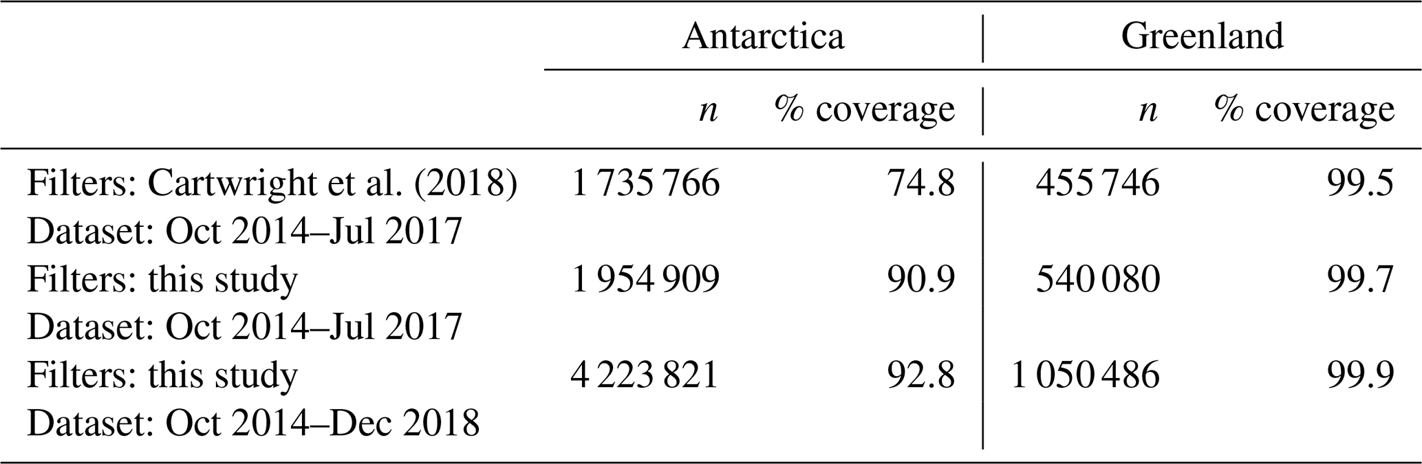
Over Antarctica, the methods used here give coverage of an additional 18 % of Antarctica's glacial ice area (Table 1) and a decrease of 45 % (9 m) in interpolated median error to 10.4 m, as shown in Table 2, when compared to Cartwright et al. (2018). The RMSE of the DEM (gridded error) shows a decrease of 115 m, as shown in Table 3. This recalculated DEM can be seen in Fig. 1. Comparisons of data south of 88^∘ S with available Operation IceBridge (Studinger, 2013) data yields RMSEs of less than 33 m (Table 4).

Table 2 Comparison of interpolated error using method of Cartwright et al. (2018) and those presented in this study, both for Antarctica and Greenland, applied across the entire dataset of TDS-1, using data between October 2014 and December 2018. The TDS-1 Antarctic DEM (a) is compared with the CryoSat-2 v1 1 km DEM (Slater et al., 2018), the DEM by Bamber et al. (2009), and the surface elevation data from Bedmap-2 (Fretwell et al., 2013). The Greenland DEM (b) is compared with the GL-CCI, Bamber (2001), and Howat et al. (2014).

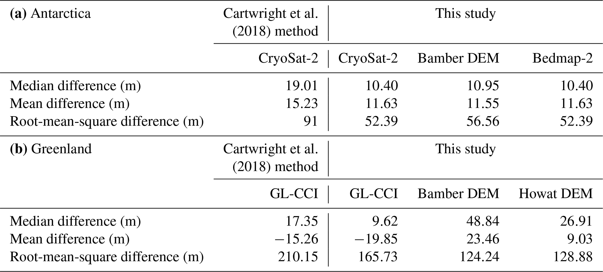
Table 3 Comparison of gridded data between the method of Cartwright et al. (2018) and those presented in this study, both for Antarctica and Greenland, applied across the entire dataset of TDS-1, using data between October 2014 and December 2018. The TDS-1 Antarctic DEM (a) is compared with the CryoSat-2 v1 1 km DEM (Slater et al., 2018), the DEM by Bamber et al. (2009), and the surface elevation data from Bedmap-2 (Fretwell et al., 2013). The Greenland DEM (b) is compared with the GL-CCI DEM, that of Bamber (2001), and that of Howat et al. (2014).

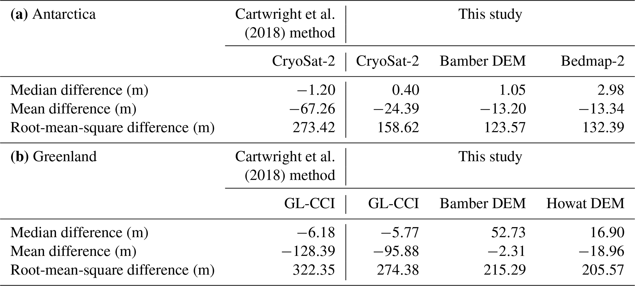
Table 4 Comparison of error with Operation IceBridge elevation estimates, (Studinger, 2013). N= 2 841 200 289 and N= 3 889 345, respectively, for continent-wide comparisons and those greater than 88^∘ S.

4 Comparison against CryoSat-2 and GL-CCI

As presented in Fig. 1, altimetry using GNSS-R is feasible over glacial ice and is capable of giving measurements over the South Pole itself, which is as yet unavailable for measurement with existing satellite altimetry techniques. Interpolated and gridded errors when compared to other DEMs are presented in Tables 2 and 3 respectively. The DEM product results in a median difference over Antarctica of 40 cm in comparison to the most recent version of the CryoSat-2 DEM and under 6 m over Greenland when compared to GL-CCI (Table 3). This higher error over Greenland is to be expected considering the higher ratio of steep coastline to inland ice sheet, as higher inclinations have been found to be associated with increased error, in agreement with Cartwright et al. (2018). Data on slope effects can be found in the Supplement. This is in part due to corner reflection effects giving multiple DDM peaks and error in the estimation of the specular point location, with surface slope not accounted for in the location calculation, as it is largely dependent on the roughness of the reflecting surface and its alignment with the look angle of the satellite. In addition, in Greenland the higher error in these regions may be due to the high slopes of the coastal terrain resulting in rocky outcrops, rather than glacial ice. In this respect it may be considered similar to the Antarctic Peninsula, and thus the errors are comparable. These patterns can be seen in Fig. 2, with higher errors around the coastlines and in the more mountainous regions of the ice sheet interiors. These points account for the majority of the underestimations appearing near the origin in Fig. 3 and are a source of discrepancies between the comparison DEMs themselves, especially where Greenland is concerned. It is these areas that give the large error ranges seen in Figs. 2 and 3.

Figure 1 Digital elevation models for the (a) Antarctic and (b) Greenland ice sheets. Elevations shown are metres above the ellipsoid, with white denoting no available data, gridding in 25 km cells, and coastlines shown in black.

Comparisons with IceBridge data south of 88^∘ were somewhat limited due to the remoteness of the location for surveying. However, the results show RMSEs of less than 33 m. When compared across the full extent of the Antarctic ice sheet, this increases to 136 m, primarily due to the inclusion of steeply sloping ice sheet margins (Table 4).

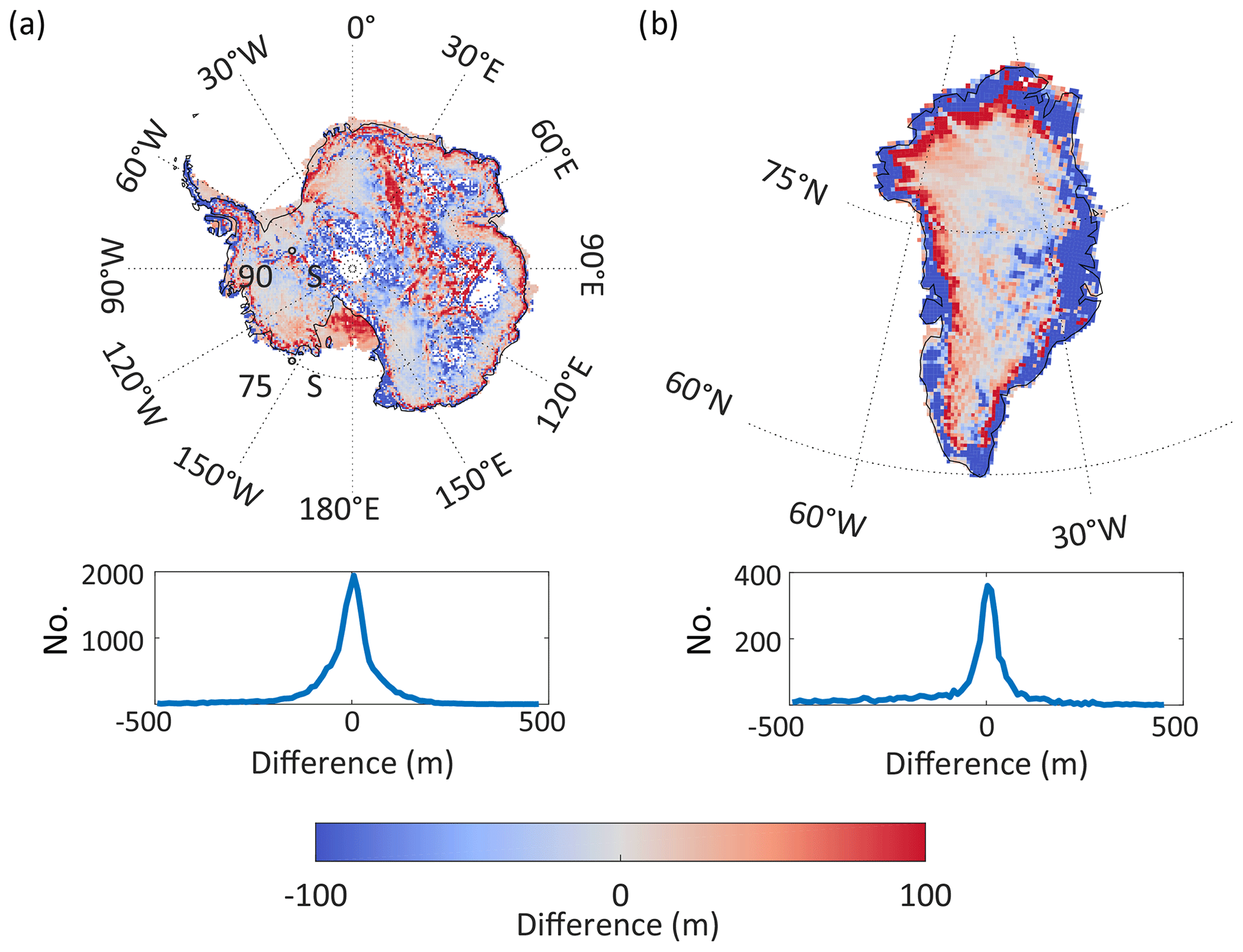
Figure 2 Error maps over (a) Antarctica and (b) Greenland with respective histograms. The error shown is the comparison DEM subtracted from TDS-1 DEM. Comparison DEMs are the CryoSat-2 v1 1 km DEM (Slater et al., 2018) and the GL-CCI for (a) and (b), respectively.

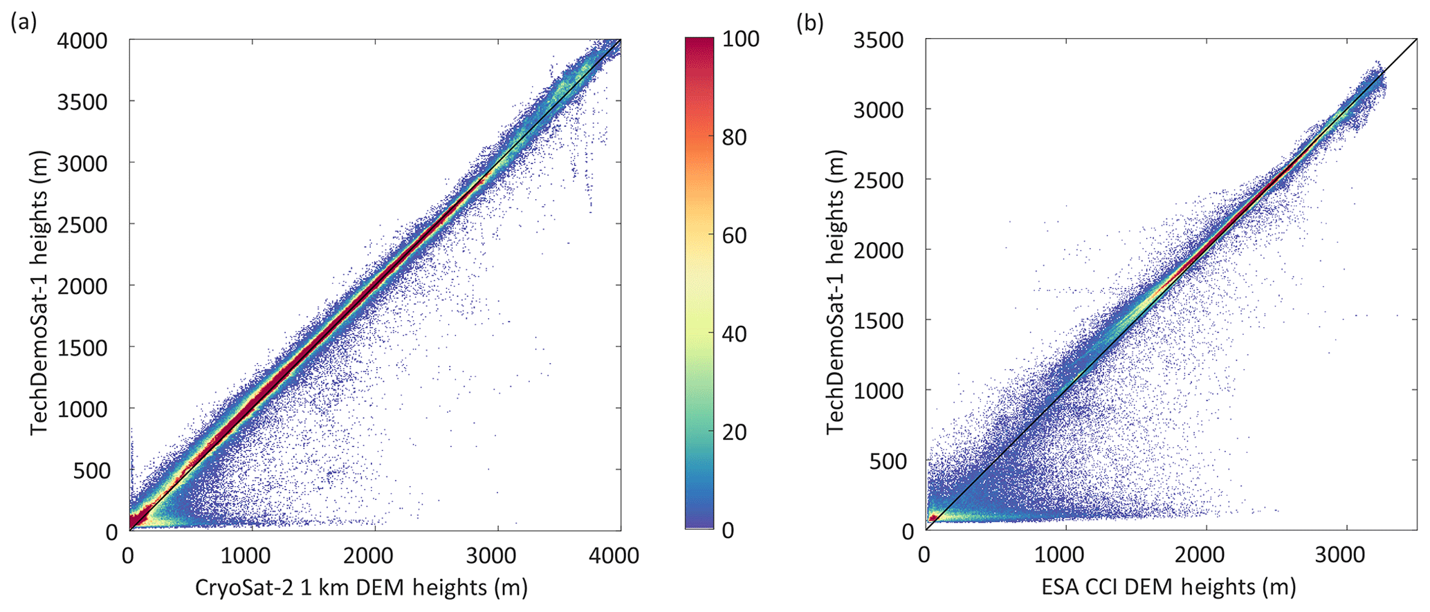
Figure 3 Density plot comparing height estimations from TechDemoSat-1 over (a) Antarctica and (b) Greenland and co-located data from the CryoSat-2 v1 1 km DEM (Slater et al., 2018) and the GL-CCI, respectively, with a 1 : 1 reference line (black).

When gridded at finer resolutions, accuracy of the resultant DEM increases; however, this results in a reduction in the spatial coverage. This suggests that reflections are from a small area and are in agreement with the theory that states that the footprint of the SGR-ReSI should be small, at approximately 6 km along-track by 0.4 km across track over sea ice (Alonso-Arroyo et al., 2017). Whilst reflections from glacial ice are expected to be less coherent and therefore produce a larger footprint, it is still expected to be less than the grid cell size used. Due to the nature of the platform as a demonstration mission and the design of the system for other measurements, it is necessary to grid the DEMs at this low resolution so as to avoid too many gaps in the data. However, it is promising for future applications of this technology that higher resolution seems to be limited by data availability rather than sensor footprint size.

There are a number of known issues with the TDS-1 dataset, including the uncertainty of the orbit and attitude of the satellite itself. These are covered in detail by Foti et al. (2017) and Clarizia and Ruf (2016). Attitude information is acquired from sun sensors; however, when in eclipse this is retrieved from magnetometers with higher uncertainty (at times up to 10^∘, Foti et al., 2017). Large changes in attitude are found in the data when exiting eclipse. However, the error patterns seen here show no obvious relationship to these fluctuations.

The data considered here include those collected in both Automatic Gain Control Mode (November 2014–April 2015) and Fixed Gain Mode (April 2015–December 2018). A strength of the elevation algorithm used here is that it is robust to fluctuations in absolute power levels caused by such changes in mode of acquisition, due to its use of the shape of the waveform and the power relative only to its peak. This is especially valuable as the power received by TDS-1 is uncalibrated with respect to that transmitted from the GPS satellites and not normalized for antenna effects.

The different averaging methods employed for all DEMs produced and used as comparisons here are likely to result in errors when compared to one another. Seasonality and shorter timescale temporal changes were considered; however, they were not found to be connected to the discrepancies between the datasets (results not shown).

5 Discussion of the benefits and limitations of the technique

In addition to the novelty of measurements over the geographic poles, which were previously not possible with satellite altimetry, the primary benefits of this technique result from the low power and mass of the receiver. These mean that a low-cost multi-satellite mission is feasible and has the potential to increase the spatial and temporal resolution of observations far beyond those in the present study. The use of a technology demonstration mission limits the data available here, and if this technique were to be exploited using dedicated platforms designed for these measurements, a significant increase in the available data could be expected. For example, the continuous operation of a single sensor would lead to a 300 % increase in data as compared to the initial TDS-1 mission. If, in addition, a larger number of reflections were to be tracked at once, this would also multiply the data available, giving a manyfold increase in the spatio-temporal resolution of products. As seen in this study, the higher resolution of the product gives an increase in accuracy, indicating that the footprint of the measurements is not the limiting factor on the resolution of the data product, but instead this factor is the quantity of data available. This results in a compromise necessary to maximize coverage over the area of interest. A dedicated mission would require a full error budget appraisal, accounting for corrections required due to the design of the sensor and the auxiliary measurements necessary to enable these. It is likely, in addition, that a dedicated mission could also collect phase information from the reflected signals in order to greatly improve the accuracy of the height retrievals, as seen in Hu et al. (2017) and Li et al. (2017).

Here we detail sources of error and limitations of this dataset. Due to the unknown physical properties of the material, the penetration of L band into snow and/or ice is a significant unknown (Passalacqua et al., 2018). This is primarily due to the wide range of electromagnetic changes snow and ice undergo in terms of varying densities and precipitation regimes as the snow is compacted and the glacial ice is formed, with both the sub-surface properties and those of the snow on top affecting the signal (Brucker et al., 2014; Leduc-Leballeur et al., 2017). Cardellach et al. (2012) measured the penetration of GNSS signals of up to 300 m over dry snow in Antarctica, whilst similar studies at L band over glacial ice in Greenland have yielded between 3 and 120 m of penetration depending on the terrain (Li et al., 2017; Mätzler, 2001; Rignot et al., 2001). These corrections are not applied to the dataset here due to the unknown characteristics of the ice and snow at the time of the retrieval. An additional factor is the atmospheric uncertainties at high latitudes, resulting in ionospheric and tropospheric effects on the signal. These are thought to introduce errors of around 10 m at the equatorial maximum (Hoque and Jakowski, 2012), with errors being smaller at higher latitudes, and thus these are much smaller than the error magnitudes found here (assuming that the comparison DEMs are “truth”, but they too, of course, contribute to the RMSEs).

6 Conclusions

This study demonstrates that high-resolution bi-static altimetry of ice sheets is possible with GNSS-R in both hemispheres to an accuracy of under 10 m when compared to contemporary elevation models. With increased data availability through dedicated GNSS-R missions and sensors designed for the purpose, high-resolution altimetry of the polar areas, including the region surrounding the South Pole, would be possible at a higher resolution than that obtained here, where it is limited primarily by data availability. As the platform only requires a receiver, this technique is inexpensive, lightweight, and low power, lending itself to a constellation configuration. Future proposals, such as G-TERN (Cardellach et al., 2018), present the concept of a constellation similar to CYGNSS with a polar focus. Such a mission would allow further increases in the spatio-temporal resolution of the measurements, and through this allow measurements of even the most dynamic aspects of the cryosphere. The feasibility of such a mission would depend on the detailed error budget for the measurements (beyond the scope of this paper). Accuracies may be increased further through the use of phase delay information (Cardellach et al., 2004; Li et al., 2017) and interferometric techniques. In addition, constraining specular point locations and improved modelling of the signal within the ice sheet will also improve estimates.