Satellite observations of unprecedented phytoplankton blooms in the Maud Rise polynya, Southern Ocean

The appearance of phytoplankton blooms within sea ice cover is of high importance considering the upper ocean primary production that controls the biological pump, with implications for atmospheric CO₂ and global climate. Satellite-derived chlorophyll a concentration showed unprecedented phytoplankton blooms in the Maud Rise polynya, Southern Ocean, with chlorophyll a reaching up to 4.67 mg m⁻³ during 2017. Multi-satellite data indicated that the bloom appeared for the first time since the entire mission records started in 1978. An Argo float located in the polynya edge provided evidence of bloom conditions in austral spring 2017 (chlorophyll a up to 5.47 mg m⁻³) compared to the preceding years with prevailing low chlorophyll a. The occurrence of bloom was associated with the supply of nutrients into the upper ocean through Ekman upwelling (driven by wind stress curl and cyclonic ocean eddies) and improved light conditions of up to 61.9 einstein m⁻² d⁻¹. The net primary production from the Aqua Moderate Resolution Imaging Spectroradiometer chlorophyll-based algorithm showed that the Maud Rise polynya was as productive as the Antarctic coastal polynyas, with carbon fixation rates reaching up to 415.08 mg C m⁻² d⁻¹. The study demonstrates how the phytoplankton in the Southern Ocean (specifically over the shallow bathymetric region) would likely respond in the future under warming climate conditions and continued melting of Antarctic sea ice.

1 Introduction

Antarctica sea ice moderately increased during the satellite era from 1979 to 2015, with regional heterogeneity that comprises both increasing and decreasing patterns in different sectors (Turner et al., 2017). However, anomalously record low sea ice extent and area were observed for three successive years from 2016 to 2018 with the maximum melting occurring in 2017 (Parkinson, 2019). Amid the pronounced melting, the largest and most prolonged Maud Rise (MR) open ocean polynya since the 1970s reappeared on 14 September 2017 ($\sim \mathrm{9.3}\times {\mathrm{10}}^{\mathrm{3}}$ km²) and expanded to a maximum on 1 December 2017 ($\sim \mathrm{298.1}\times {\mathrm{10}}^{\mathrm{3}}$ km²) and existed for 79 d (Jena et al., 2019). Appearance of the polynyas plays an important role in the oceanic phytoplankton and primary production that control the biological pump of the ocean (Arrigo and Dijken, 2003; Shadwick et al., 2017), as well as being important for marine mammals and birds (Labrousse et al., 2018; Stirling, 1997), global heat and salt fluxes (Tamura et al., 2008), Antarctic bottom water properties (Zanowski et al., 2015), and atmospheric circulation (Weijer et al., 2017). However, due to their spatial dimension, the polynyas are generally not represented well in large-scale climate models, limiting the capability of simulating and projecting polynya-related biophysical changes under a future climate change scenario (Li et al., 2016).

The Southern Ocean (SO) is known as the largest high-nutrient low-chlorophyll (HNLC) area of the global ocean. For the past 50 years, the loss of ice shelves and glacier retreat around the Antarctic Peninsula have increased, and at least 24 000 km² in surface area of new open water was rapidly colonized by new phytoplankton blooms, with new benthic and marine zooplankton communities in the SO (Peck et al., 2010). In the background of HNLC, the occurrence of polynyas can enhance the chlorophyll a (chl a) concentration (a proxy for phytoplankton biomass) due to the increase in surface area of new open waters and growth season of the phytoplankton (Kahru et al., 2016). The bloom occurrence in the SO has been linked with oceanographic features such as jet streams, meanders, and mesoscale eddies, which can lead to increased iron and silicate supply by the ocean upwelling (Strass et al., 2002), thereby improving co-limitation of nutrient and light for phytoplankton growth (Hoppe et al., 2017). Oceanic eddies have been found to regulate chl a variability in the SO, with higher (lower) values observed for the cyclonic (anticyclones) eddies (Kahru et al., 2007). The polynyas of the Amundsen and Ross seas have high primary productivity that contributes to the SO carbon dioxide (CO₂) sink (Alderkamp et al., 2012; Arrigo et al., 2008a; Arrigo and Alderkamp, 2012; Yager et al., 2012). The primary productivity of these regions reaches up to 3 g C m⁻² d⁻¹, roughly 10-fold more than the SO mean productivity (Arrigo and Dijken, 2003). The high productivity values in the polynya have been attributed to the supply of iron from the upwelling of iron-rich deep water (Planquette et al., 2013), sediment diffusion or resuspension followed by upwelling (Ardelan et al., 2010), atmospheric inputs (Cassar et al., 2007; Wagener et al., 2008), melting of sea ice (Lannuzel et al., 2010; van der Merwe et al., 2011), iceberg-delivered glacial debris (Raiswell et al., 2008), and melting of ice shelves (Pritchard et al., 2009; Wåhlin et al., 2010). The Amundsen polynya is one of the productive polynyas of Antarctica with satellite-derived chl a (2.2 mg m⁻³) 40 % greater than in the Ross Sea polynya (1.5 mg m⁻³) (Schofield et al., 2015). Although the polynyas are believed to be the sites of phytoplankton blooms in spring (Arrigo and Dijken, 2003), and they act as sinks of atmospheric CO₂ because of both physical–chemical processes and biological activity (Bates et al., 1998; Mu et al., 2014), very little is known about the MR polynya due to its rare appearance. In this paper, we report the first evidence of the occurrence of phytoplankton bloom in the MR polynya from satellite-derived ocean color data and the Argo float. Further, the role of physical processes in the occurrence of bloom in the polynya is examined using relevant physical oceanographic data, followed by bloom occurrence's likely implication for ocean–atmosphere exchange of CO₂.

2 Materials and methods

In order to understand the impact of bathymetry on the phytoplankton biomass, the MR seamount was mapped using bathymetric raster data (21 601×10 801 pixels) from the Earth Topography One Arc-Minute Global Relief Model, 2009 (ETOPO1) (https://www.ngdc.noaa.gov/, last access: 21 March 2020). The raster data were converted to polyline features with a contour interval of 500 m for showing the extent of the seamount (Fig. 1a). A level-3 monthly composite of satellite-derived near-surface chl a imageries from the Nimbus-7 Coastal Zone Color Scanner (CZCS), Sea-viewing Wide Field-of-view Sensor (SeaWiFS), Aqua Moderate Resolution Imaging Spectroradiometer (Aqua MODIS), and Visible Infrared Imaging Radiometer Suite (VIIRS) were used, as per the availability of data from 1978 to 2017 (Fig. 1b–e). Level-2 Aqua MODIS ascending passes were processed (relatively cloud-free data) to generate the high-spatial-resolution (∼1 km) chl a images on 25 October (14:45 UTC), 6 November (15:05 UTC), and 21 November 2017 (14:25 UTC) (Fig. 2). We used a standard chl a retrieving algorithm that uses a combination of both lower and higher ranges of chl a retrieval as described in the Algorithm Theoretical Basis Document (ATBD) from the NASA Earth Observing System Project Science Office (https://oceancolor.gsfc.nasa.gov/atbd/chlor_a/, last access: 21 March 2020). In this study, we have used the criteria of chl a>0.8 mg m⁻³ (Fitch and Moore, 2007) for defining a phytoplankton bloom after considering the underestimation tendency of chl a measurement from satellite observations over the Southern Ocean (Jena, 2017).

In order to analyze the Aqua-MODIS-derived net primary production (NPP), we have validated three ocean-color-based models such as the vertically generalized production model (VGPM), Eppley-VGPM, and carbon-based productivity model (CbPM) for selecting the best model for the study region. We evaluated the performance of these models by comparing with the in situ NPP estimated using ¹³C tracer during the Indian scientific expedition to the Southern Ocean in 2009. The locations of in situ NPP observations during the austral summer (February to April 2009) are presented in Fig. 3a. The in situ NPP from 11 observations ranges from about 85.04 to 923.83 mg C m⁻² d⁻¹. The detailed method of ¹³C measurement was documented in previous work (Gandhi et al., 2012). The VGPM was developed to estimate the NPP from chlorophyll concentration after considering the influence of temperature on the efficiency of chlorophyll-specific photosynthesis. (Behrenfeld and Falkowski, 1997b). The Eppley-VGPM makes use of an exponential function developed from changes in growth rates of phytoplankton over varied temperature ranges for a wide variety of species (Eppley, 1972). Further, a new CbPM model was developed that uses backscattering coefficients and chlorophyll-to-carbon ratios for estimation of phytoplankton carbon biomass and phytoplankton growth rates, respectively (Westberry et al., 2008). The model-based NPP values were available on a weekly timescale with a spatial resolution of ∼4 km. The pixel values from the models were extracted around each in situ observation of NPP to generate the matchups for the validation strategy, a method adopted by several authors (Jena, 2017; Johnson et al., 2013). The comparative statistical analysis suggested that the scatters were much better in the case of Eppley-VGPM-estimated NPP (Fig. 3c) than those in the case of VGPM (Fig. 3b) and CbPM (Fig. 3d). A bias of −26.21 mg C m⁻² d⁻¹ for the Eppley-VGPM-obtained NPP value was much better than that obtained from the VGPM (bias = 104.40 mg C m⁻² d⁻¹) and CbPM (bias = 94.14 mg C m⁻² d⁻¹) (Table 1). The NPP values from VGPM and CbPM indicated significant overestimations. The coefficient of correlation (r) and standard error (SE) for Eppley-VGPM NPP values (r=0.82 and SE=116.16 mg C m⁻² d⁻¹) were better than those obtained from the VGPM (r=0.82 and SE=203.69 mg C m⁻² d⁻¹) and CbPM (r=0.66 and SE=142.84 mg C m⁻² d⁻¹). Results suggested the Eppley-VGPM-based NPP values match reasonably well with the in situ NPP. Therefore, we used the Eppley-VGPM model for the present study, taking Aqua MODIS as the input.

Table 1 Validation of ocean-color-based models (VGPM, Eppley-VGPM, and CbPM) with in situ net primary production (mg C m⁻² d⁻¹) estimated using ¹³C tracer during the scientific expeditions to the Southern Ocean in 2009. CbPM: carbon-based productivity model; VGPM: vertically generalized production model.

We used monthly sea ice concentration (SIC) data (September to November 2017) from the Special Sensor Microwave Imager/Sounder (SSMIS) with spatial resolution of 25 km acquired from the National Snow and Ice Data Center (NSIDC) (data ID G02135, version 3). The data were generated using the NASA Team algorithm, which converts satellite-derived brightness temperatures to gridded SIC (Cavalieri et al., 1997). A detailed description of the sensor characteristics, sea ice processing methods, synoptic coverage, resolution, projection, and validation of sea ice retrieval from passive microwave sensors is given in earlier work (Fetterer et al., 2016). The polynya was assumed when the pixel values were found to be less than or equal to 15 % of SIC (Fig. 4a–c) (Jena et al., 2019). In order to examine the role of oceanic processes in the formation of the phytoplankton bloom in the polynya, we used relevant physical oceanographic data. Metop Advanced SCATterometer (ASCAT) wind stress curl and Ekman upwelling data (Pond and Pickard, 1983) were acquired from the National Oceanic and Atmospheric Administration (NOAA) Coast watch (https://coastwatch.pfeg.noaa.gov, last access: 21 March 2020) at a spatial resolution of $\mathrm{0.25}{}^{\circ }\times \mathrm{0.25}{}^{\circ }$ (Fig. 4g–l). Oceanic eddies were identified from the sea surface height anomaly (SSHA) and geostrophic currents ($\mathrm{0.25}{}^{\circ }\times \mathrm{0.25}{}^{\circ }$) derived from multi-mission merged satellite altimeter data (https://las.aviso.altimetry.fr/, last access: 21 March 2020) (Fig. 4d–f) (Jena et al., 2019). Although the dipole structure of cyclonic and anticyclonic eddies was observed in the MR polynya, cyclonic eddies dominated the flow pattern in the region during the event. Therefore, we focused on the cyclonic eddies because they can upwell the deep, warm and nutrient-rich water to the upper ocean for chl a enhancement. The optimal interpolated sea surface temperature (OI SST) data (9 km × 9 km) were obtained from Remote Sensing Systems (http://www.remss.com/, last access: 21 March 2020) and were produced after merging the microwave (cloud penetration capabilities) and infrared SST (high spatial resolution) using an OI scheme (Reynolds and Smith, 1994) (Fig. 4m–o). In order to understand the vertical structures of biophysical parameters, we used Argo float (ID-5904468) data that had remained in the MR polynya from 2015 to 2017 (http://www.argo.ucsd.edu/, last access: 21 March 2020) (Fig. 1a). The Argo-based partial pressure of CO₂ (pCO₂) in the water column was calculated from a Deep-Sea DuraFET pH sensor after using an existing algorithm for total alkalinity (Johnson et al., 2016). The uncertainty in the derived value is about 11 µatm at pCO₂ of 400 µatm (∼2.7 %), considering the combined contribution from the pH sensor, the alkalinity estimate, and carbonate system equilibrium constants (Williams et al., 2017). The monthly net shortwave radiation was acquired from the European Centre for Medium-Range Weather Forecasts (ECMWF) (grid resolution of 0.25^∘) during January 1979–December 2017. Monthly anomalies of shortwave radiation for September–November 2017 were computed relative to a 38-year climatology (1979–2016).

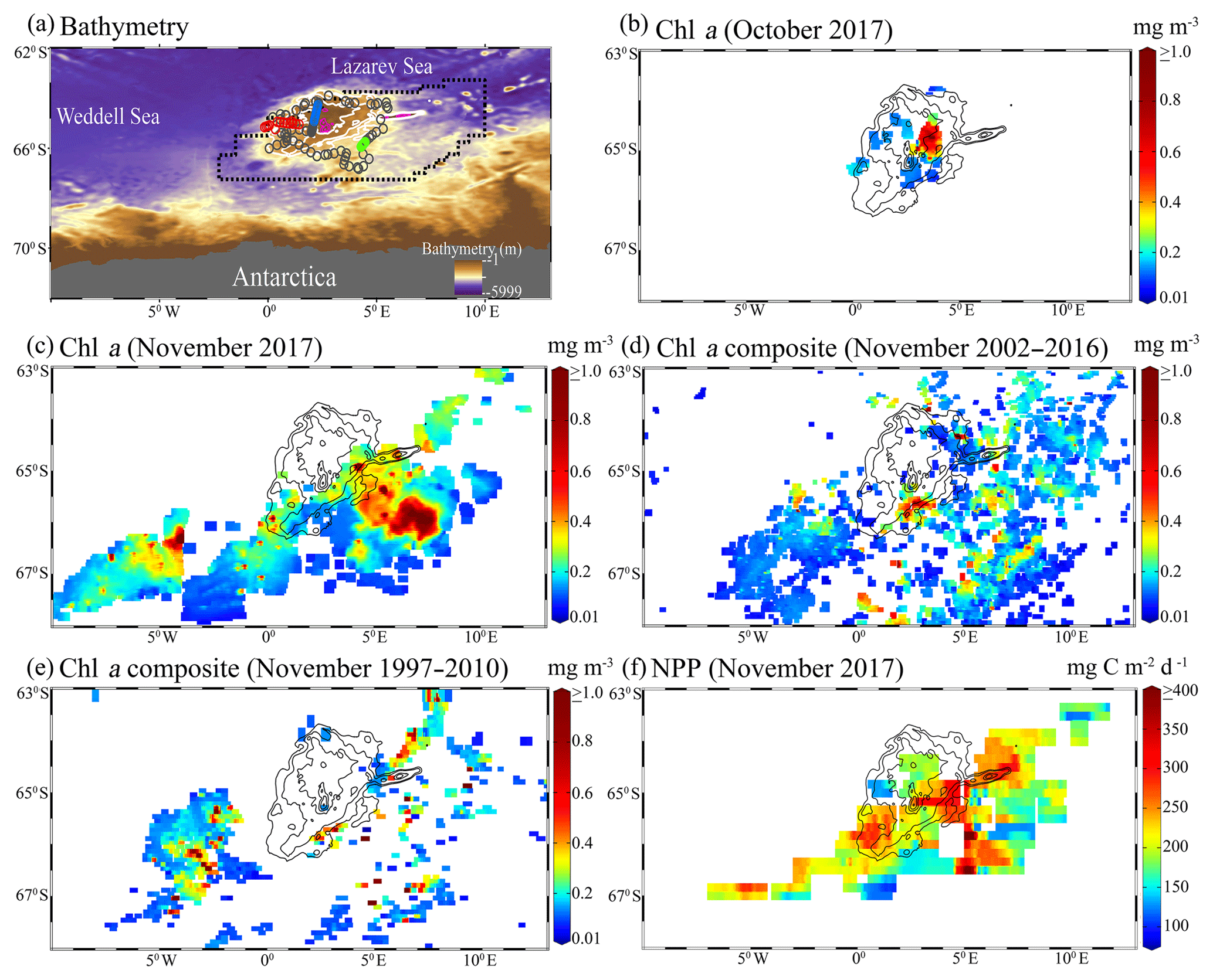
Figure 1 (a) Bathymetry map of the Maud Rise from the Earth Topography One Arc-Minute Global Relief Model, 2009. Pink lines show the depth contours shallower than 2000 m, and other white contours are spaced by 500 m with deeper values. The dashed polygon shows the extent of the polynya on 21 November 2017. Circles represents the location of an ARGO float (ID-5904468) from 19 January 2015 to 18 March 2018. Red, green, and blue circles show the float location from August to December for 2017, 2016, and 2015, respectively. (b) Monthly mean chlorophyll a (chl a) from the Aqua Moderate Resolution Imaging Spectroradiometer (Aqua MODIS) during October 2017. (c) Monthly mean chl a from Aqua MODIS during November 2017. (d) Long-term composite of Aqua MODIS chl a (2002–2016) for November. (e) Long-term composite of SeaWiFS chl a (1997–2010) for November. (f) Monthly mean daily net primary productivity (NPP) computed from the Eppley vertically generalized production model for November 2017. The polyline features in (b–f) show the extent of the Maud Rise seamount with a contour interval of 500 m.

3 Results and discussion

3.1 Phytoplankton bloom within the polynya

Although a large polynya was formed within the MR sea ice cover during September 2017, no phytoplankton bloom is observed in the satellite record. The polynya extent was nearly static from September to October and accompanied by a small patch of bloom (chl a up to 3.48 mg m⁻³) centered at 3.77^∘ E and 64.72^∘ S (Figs. 1b; 4b), which remains otherwise covered by the sea ice. Prior to the October 2017 event, no chl a was observed for the month of October from 1978 to 2016 even after considering the entire data records of CZCS, SeaWiFS, Aqua MODIS, and VIIRS. During November 2017, the polynya was enlarged and shifted southeastward with high chl a concentration reaching up to 4.66 mg m⁻³ (Figs. 1c; 4c). The bloom was formed approximately between 64.5–66.5^∘ S and 4–8^∘ E. Prior to the November 2017 event, satellite-derived chl a observations were scarce (SeaWiFS and MODIS) and missing (CZCS and VIIRS) for the month of November from 1978 to 2016. Figure 1d and e show the climatological composite of chl a observations in November for Aqua MODIS (2002–2016) and SeaWiFS (1997–2010), respectively. The scarce and missing observations were mainly due to the presence of seasonal sea ice cover and cloud cover in the MR. The result suggests that the observed bloom from October to November 2017 had appeared for the first time within the MR polynya in the records of satellite observations since 1978 (Fig. 1b–c). Even though the monthly composite images show the evidence of blooms, we processed level-2 high-spatial-resolution scenes of Aqua MODIS that provided more information on this unprecedented phytoplankton bloom. Several selected scenes that have relatively better coverage showed a patch of bloom on 25 October, followed by a wide band of bloom on 6 and 21 November 2017 (Fig. 2). The chl a values reached as high as 4.67 mg m⁻³ on 6 November 2017 (Fig. 2b). A high diffuse attenuation coefficient (Kd 490) of up to 0.39 and 0.37 m⁻¹ was observed during October and November, respectively, which is an indicator of sediment resuspension and bloom conditions in the MR polynya (Table 2). The previously reported highest chl a concentration in the Antarctic polynya was identified in the Amundsen Sea (coastal polynya) with values reaching about 6.98 mg m⁻³ (Arrigo and Dijken, 2003). The bloom in the MR polynya was also tracked by a robotic Argo float (ID-5904468) that had remained at the northwestern edge of the polynya (Figs. 1a; 5a). Results show enhanced chl a values from September to November 2017. The bloom condition was initiated on 25 October 2017 with chl a maxima of up to 1.27 mg m⁻³ (36 m depth) at 0.86^∘ E and 64.98^∘ S (Fig. 5a). The chl a value reached up to 1.31 mg m⁻³ (41 m depth) and 1.73 mg m⁻³ (36 m depth), respectively on 4 and 14 November 2017. Further, on 24 November 2017, the values reached as high as 5.47 mg m⁻³ (11 m depth) at 1.43^∘ E and 65.04^∘ S. In order to check whether this observed bloom is a seasonal or an episodic feature of the MR, we analyzed the Argo float data during the 2 preceding years of 2015 and 2016 when the sea ice was covered. Analysis shows that the bloom was absent and the chl a value found to be rather low during October and November for 2015 and 2016 (Fig. 5b, c). Thus, the result confirms that the observed bloom in 2017 was an unprecedented feature considering both the Argo float and multi-sensor satellite data.

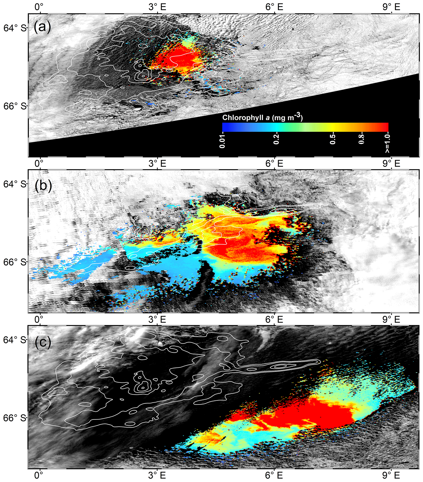
Figure 2 High-spatial-resolution (∼1 km) Aqua MODIS ascending passes on (a) 25 October (14:45), (b) 6 November (15:05), and (c) 21 November 2017 (14:25), showing the unprecedented phytoplankton blooms in the Maud Rise polynya. The white contours show the extent of the Maud Rise seamount.

3.2 Causes of the observed bloom formation

Generally, the phytoplankton biomass remains low in the SO, which is mainly ascribed to the lack of micronutrient iron apart from strong zooplankton grazing pressure and light and silicate limitation (de Baar and Boyd, 1999; Boyd et al., 2001; Gall et al., 2001; Selph et al., 2001). The input of iron-enriched atmospheric dust from the continents to the SO is the lowest in the world's oceans (Duce and Tindale, 1991). The oceanic sources of iron from the deep water and vertical diffusion of iron through the water column have been reported as likely pathways of iron supply to the upper ocean (Jena, 2016; Tagliabue et al., 2014). The occurrence of phytoplankton bloom is possible over the shallow regions of the MR seamount where the doming of the isotherm/isopycnal can bring deeper high-nutrient water above the seamount, where it may be utilized with a conducive environment of light availability and water column stability (White and Mohn, 2002). Analysis of bathymetric data indicated the peak of the MR seamount is located at 65.23^∘ S, 2.63^∘ E and rises from the abyssal plain of ∼5200 m to the shallowest depth of ∼968 m (Fig. 1a), influencing the local upliftment of thermocline and nutrient-enriched deep water (Jena et al., 2019; Mashayek et al., 2017; Muench et al., 2001; Roden, 2013). The oceanic processes that can bring subsurface nutrients to the sea surface have an important role in the formation of phytoplankton bloom. In order to examine the role of oceanic processes, we used satellite-derived physical oceanographic data as shown in Fig. 4.

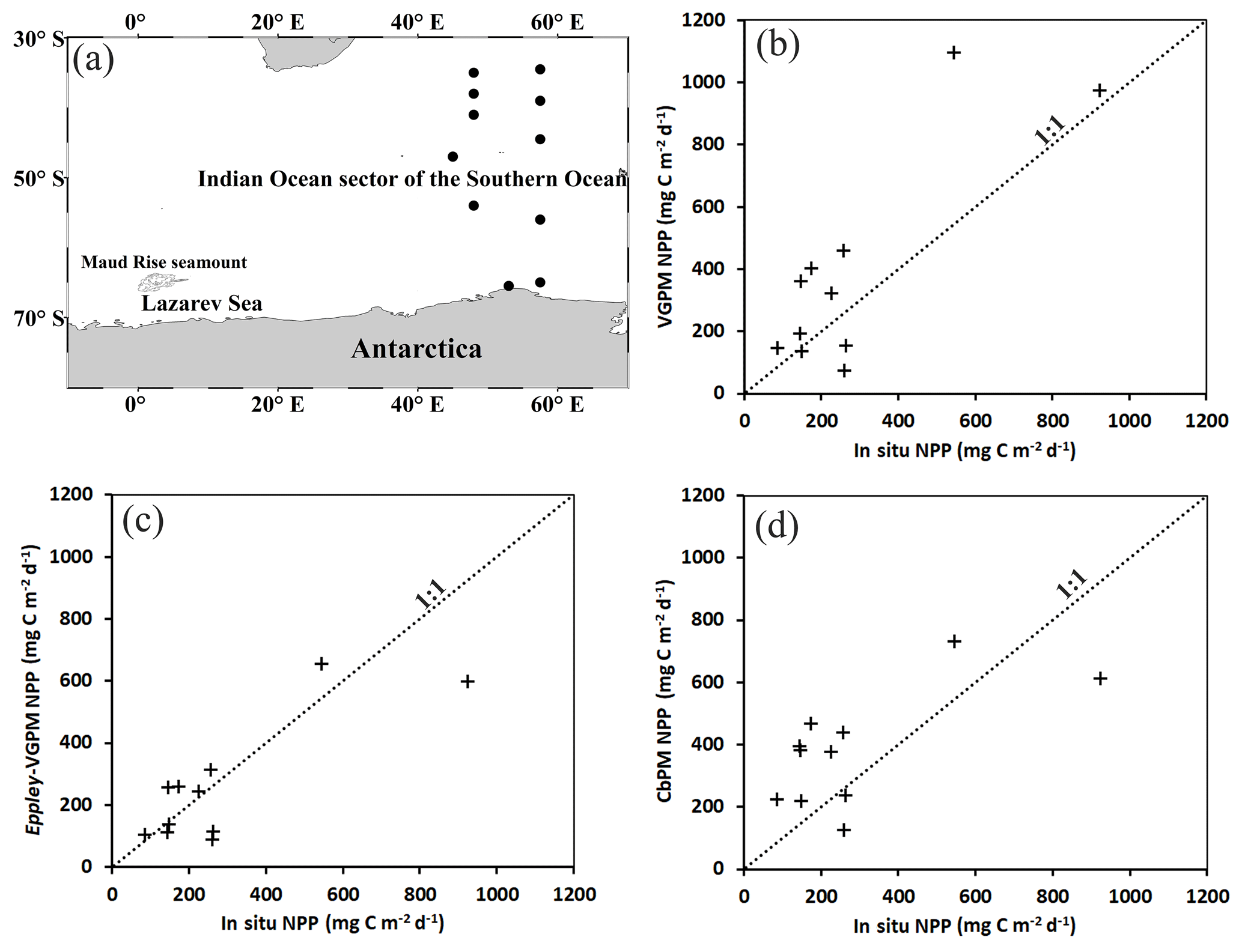
Figure 3 (a) Circles showing the locations of in situ net primary production (NPP) from the ¹³C tracer during the Indian scientific expedition to the Southern Ocean (February to April 2009). Scatter plots between in situ NPP and (b) VGPM, (c) Eppley-VGPM, and (d) CbPM NPP estimations. NPP: net primary production; CbPM: carbon-based productivity model; VGPM: vertically generalized production model.

Table 2 Net primary production and bio-optical parameters during the occurrence of the Maud Rise polynya in October and November 2017. Values for November 2017 are given within brackets. NPP: net primary production; Chl a: chlorophyll a; Eu: euphotic depth; PAR: photosynthetically available radiation; Kd: diffuse attenuation coefficient for downwelling irradiance; SST: sea surface temperature.

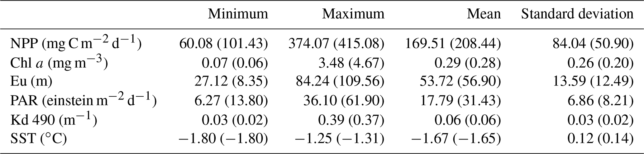
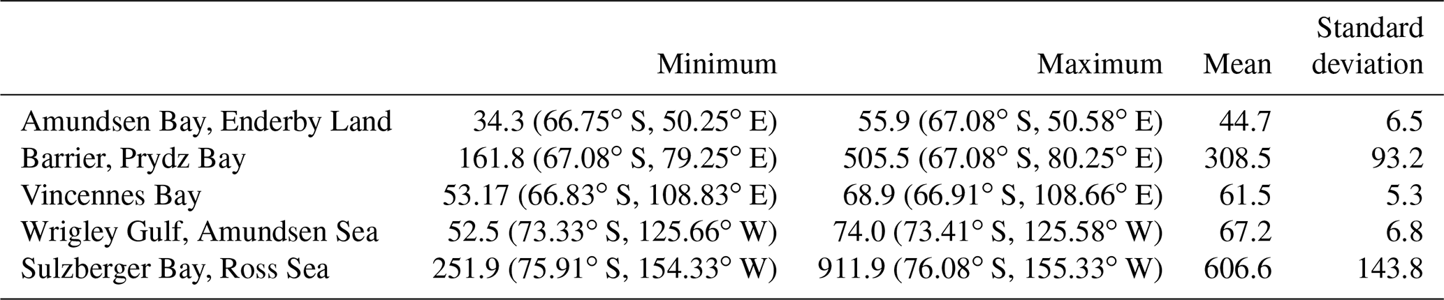
Table 3 Net primary production (mg C m⁻² d⁻¹) for some coastal polynyas around Antarctica in November 2017. The values in the parentheses indicate locational information.

Analysis of monthly SSHA and corresponding geostrophic currents showed the presence of a large cyclonic eddy with a diameter of ∼220 km in the vicinity of the MR seamount during September 2017 (Fig. 4d). The center of the cyclonic eddy was located at approximately 3.84^∘ E and 64.47^∘ S, closely matching with the center of the polynya having warm SST (−1.35 ^∘C) compared to the peripheral cold SST of −1.79 ^∘C (Fig. 4d, m). The polynya extent was nearly static from September to October. During November, the polynya expanded southeastward in conjunction with the movement of cyclonic eddy accompanied by a pool of warm SST and the phytoplankton bloom (Figs. 1c; 4f, o). The eddy was located at approximately 3.96^∘ E and 66.5^∘ S in November. Even though a dipole structure of cyclonic and anticyclonic eddies was observed in the polynya, a large cyclonic eddy dominated the flow pattern. The location of the cyclonic eddy matches well with the annular halo of warm SST and patch of phytoplankton bloom in the polynya (Figs. 1b–c; 4d–f, 4m–o). In addition, we find that the polynya surface was associated with persistent negative wind stress curl (Fig. 4g–i) that induced upwelling of subsurface water to the sea surface during September–November 2017 (Fig. 4j–l). Generally, the water column on the MR seamount is characterized by the presence of a cold fresh layer in the upper ocean separated from a lower warm saline layer by a weak pycnocline (Jena et al., 2019; de Steur et al., 2007). The combined influence of the cyclonic eddy and negative wind stress curl brings up the warm thermocline water into the sea surface through Ekman upwelling, resulting in a pool of warm SST at the polynya center (Fig. 4m–o). A depth–latitude cross section of the Copernicus Marine Environment Monitoring Service (CMEMS) global analysis and forecast data on potential temperature data at a polynya location (along 4.7^∘ E) provided evidence that the subsurface warm water was ventilated and brought closer to the upper ocean from the thermocline (upward doming of isotherms) from September through November 2017 (Jena et al., 2019). The Argo float located at the edge of the polynya also provided evidence on the uplift of thermocline during September 2017 (Fig. 6a). Ocean upwelling is known to supply dissolved iron to the upper ocean (Klunder et al., 2014; Rosso et al., 2014), preferably at the shallow bathymetry of less than 1 km at the MR seamount (Graham et al., 2015). Synchronously, along with the availability of light in October and November, the observed mechanism triggered a bloom condition in the MR polynya (Figs. 1b–c; 2a–c). The Argo float indicated mixed-layer warming on the Maud Rise during spring 2016 and 2017 (Fig. 6). The upwelling of high saline and warm water into the mixed layer facilitated the sea ice melting. The melting of sea ice leads to the development of a shallow mixed layer due to the accumulation of freshwater in the upper ocean. Therefore, we observed lower values of salinity in the mixed layer with increased stability of the water column (Fig. 6). The development of the shallow mixed layer improved the light availability in the upper ocean, and the condition was favorable for the growth of phytoplankton. Even though the Ekman upwelling was evident in September, the bloom did not appear in the polynya region under low light conditions of up to 12.6 einstein m⁻² d⁻¹. However, the bloom appeared in October–November 2017 under the influence of Ekman upwelling and improved light conditions of up to 36.1 and 61.9 einstein m⁻² d⁻¹ for October and November, respectively (Table 2). Analysis of net shortwave radiation data shows the record highest gain of values in the polynya region during September–November 2017, considering the 38-year time series from 1979 through 2016 (Fig. 7). The observed anomalous gain in net shortwave radiation is possibly due to the early loss of sea ice cover.

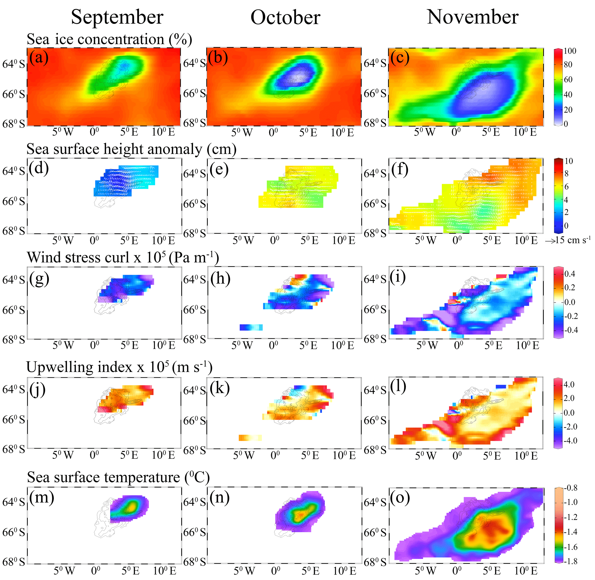
Figure 4 Monthly maps show (a–c) sea ice concentration, (d–f) sea surface height anomaly and geostrophic current velocity (white arrows), (g–i) wind stress curl, (j–l) upwelling index, and (m–o) sea surface temperature variability during the appearance of polynya from September to November 2017.

Figure 5 An Argo float (ID-5904468) located on the Maud Rise seamount shows profiles of (a–c) chlorophyll a and (d–f) pCO₂ from August to December (2015–2017). The marked rectangle in (a) shows the bloom condition from October to November 2017, and the bloom was absent during the 2 preceding years (2015 and 2016). Low pCO₂ values were observed, corresponding to the bloom occurrence.

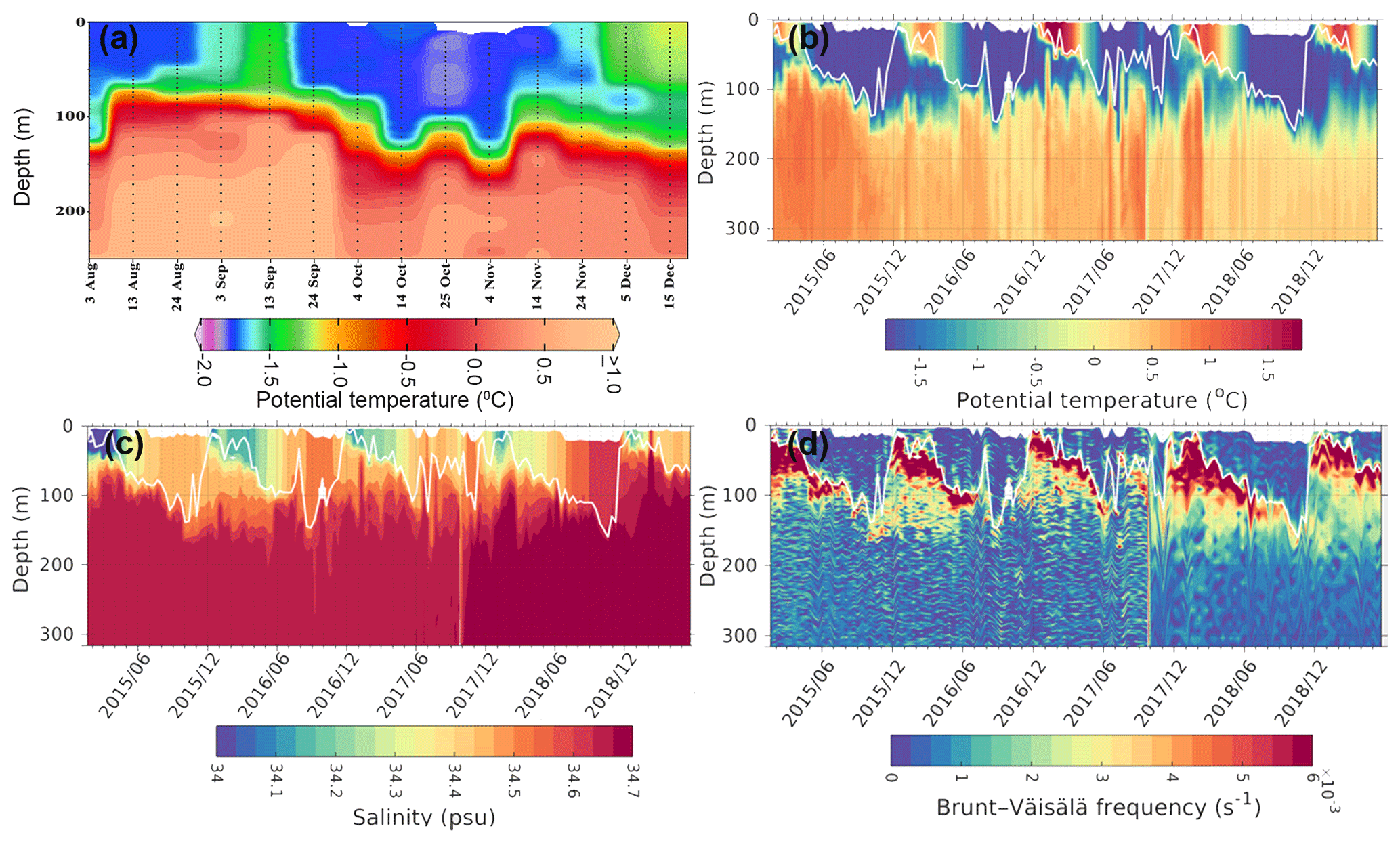
Figure 6 Profiles from an Argo float ID 5904468 located at the edge of the Maud Rise polynya show (a) potential temperature during August–December 2017, (b) potential temperature during 2015–2019, (c) salinity, and (d) static stability. The white solid line shows the variability of mixed-layer depth. The mixed layer was computed as the uppermost level of uniform potential density (σθ) at the depth where the density in the upper level varies by 0.01 kg m⁻³ with respect to the surface (Kaufman et al., 2014).

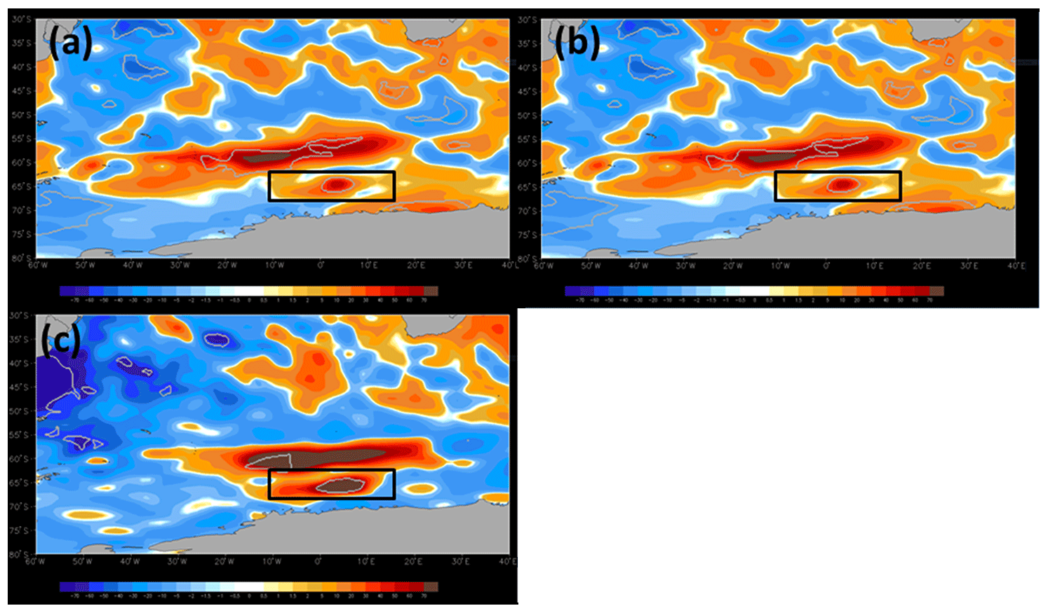
Figure 7 Monthly anomalies of net shortwave radiation (W m⁻²) for (a) September, (b) October, and (c) November 2017 in the Maud Rise polynya (black rectangles). The anomalies were computed relative to a 38-year climatology (1979–2016). The regions within grey polylines show the record level shortwave radiation in 2017 that lies outside of values from 1979 to 2016.

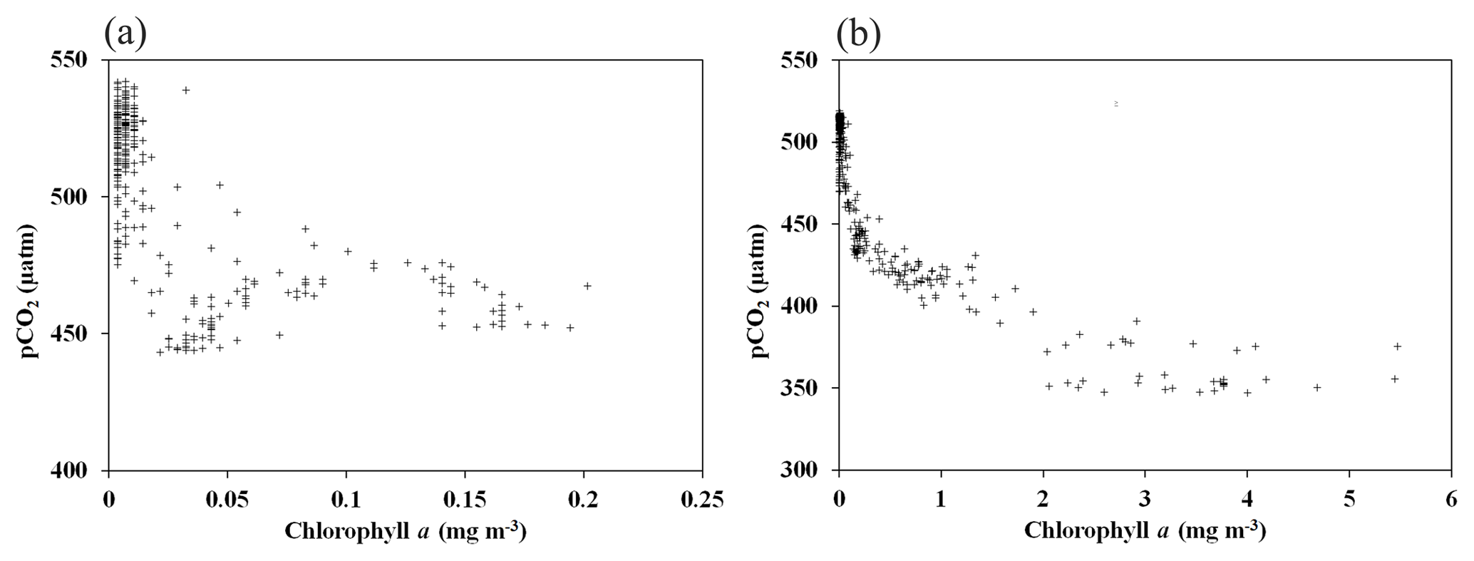
Figure 8 Argo data were utilized to find the relationship between the chlorophyll a and the oceanic pCO₂ conditions. (a) The coefficient of correlation (r) between the pCO₂ and chl a was found to be −0.56 (p<0.01) during August–September 2017. (b) The relationship improved ($r=-\mathrm{0.82}$, p<0.01) during the bloom conditions in October–November 2017.

Computation of NPP using the Eppley-VGPM model indicated the carbon fixation rates in the MR polynya varied between 60.08 and 374.07 mg C m⁻² d⁻¹, with an average value of 169.51 mg C m⁻² d⁻¹ for October 2017 (Table 2). The NPP increased in November and ranged from 101.43 to 415.08 mg C m⁻² d⁻¹, averaging 208.44 mg C m⁻² d⁻¹, with the highest rate being observed at 5.16^∘ E and 66.58^∘ S. The observed values in the polynya remained within the previously reported range for the Polar Frontal Zone of the SO (100–6000 mg C m⁻² d⁻¹) (Hoppe et al., 2017; Korb and Whitehouse, 2004; Mitchell and Holm-Hansen, 1991; Moore and Abbott, 2000; Park et al., 2010). The results from Aqua MODIS observations in the Antarctic coastal polynyas indicated that the NPP values ranged from 34.3 to 911.9 mg C m⁻² d⁻¹ during November 2017, with the highest rate being observed at the Sulzberger Bay polynya (Ross Sea) at 155.33^∘ W and 76.08^∘ S (Table 3). The NPP values in the MR polynya remained within the range of similar values observed for the coastal polynyas. The NPP values varied from 90 to 760 mg C m⁻² d⁻¹ for 37 coastal polynyas around Antarctica (Arrigo and Dijken, 2003). Even though the phytoplankton bloom appeared in the MR polynya with NPP values similar to those of coastal polynyas, the spatial variation in NPP did not always follow the same pattern of chl a (Fig. 1c, f). The observed pattern has been attributed to the effect of phytoplankton pigment composition and packaging (Bricaud et al., 2004; Ciotti et al., 2002; Jena, 2017; Lohrenz et al., 2003; Marra et al., 2007; Morel and Bricaud, 1981). The primary production in the upper ocean is a function of chl a, availability of light, nutrients, phytoplankton-specific absorption coefficient (capacity of light absorption), and efficiency of phytoplankton to convert the absorbed light for carbon fixation (Behrenfeld and Falkowski, 1997a). However, the capacity of light absorption and the quantum yield of photosynthetic carbon fixation vary from one phytoplankton community to another (Claustre et al., 2005). Although the primary production in the Antarctic coastal polynyas is known to be dominated by prymnesiophytes (Phaeocystis antarctica) or diatoms (Arrigo et al., 2008b), the data on the phytoplankton community structure and their spectral characteristics are not available for the analysis in order to quantify the rate of carbon fixation for individual communities.

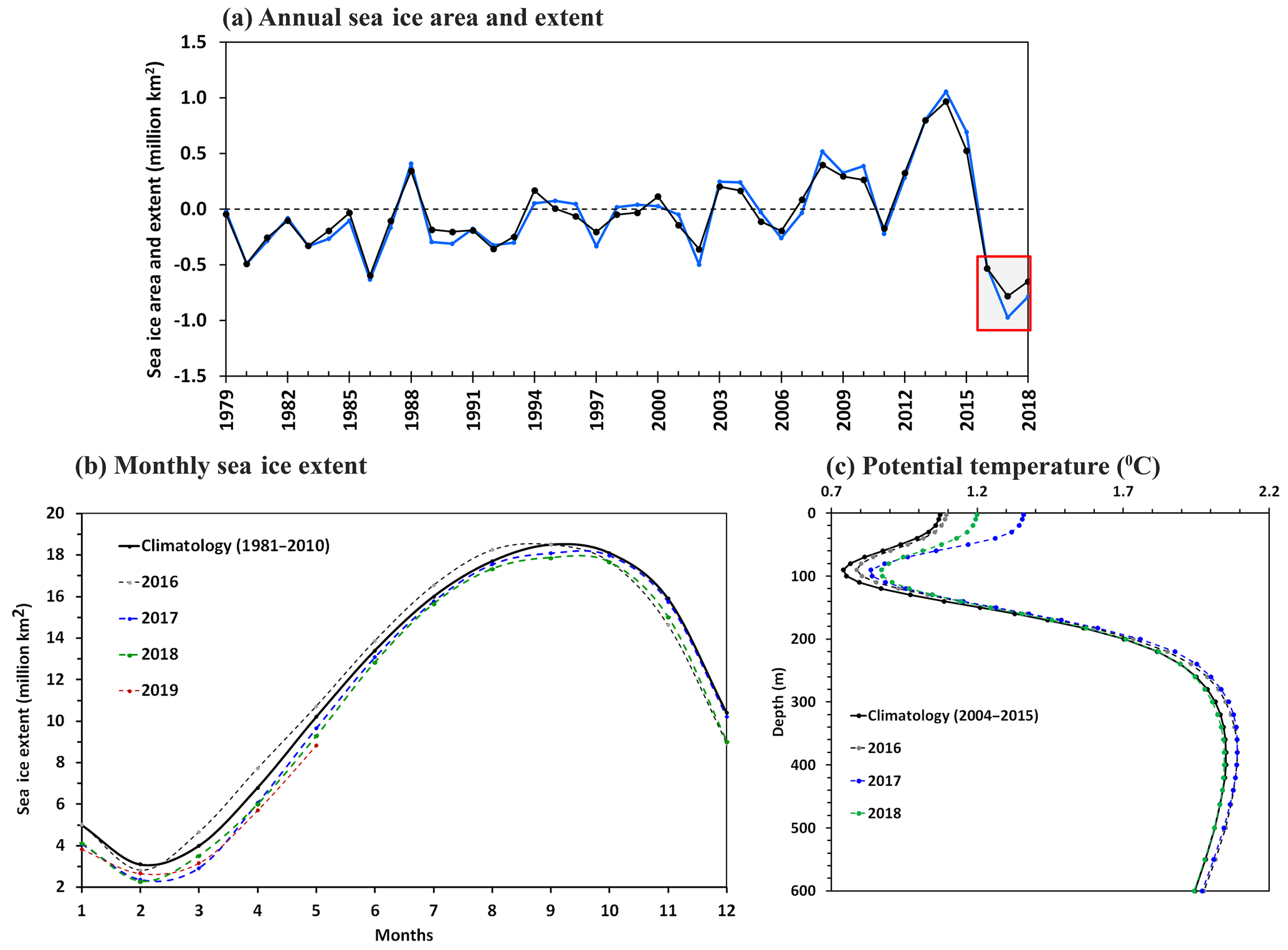
Figure 9 (a) Interannual variability of the Antarctic sea ice area (black) and extent (blue) anomaly relative to the climatology (1979–2015), as analyzed from satellite observations of passive microwave sensors. The red rectangle shows the anomalous record lowest sea ice area and extent observed for 3 successive years from 2016 to 2018, with the maximum melting occurring in 2017. (b) Monthly mean sea ice extent data indicated loss of sea ice that started from September 2016 and continued for the years 2017, 2018, and 2019. (c) Argo-based ocean potential temperature data (2004–2018) indicated anomalous upper ocean warming of the Southern Ocean from 2016 to 2018. The potential temperature was spatially averaged over the south of the 55^∘ S region encircling Antarctica.

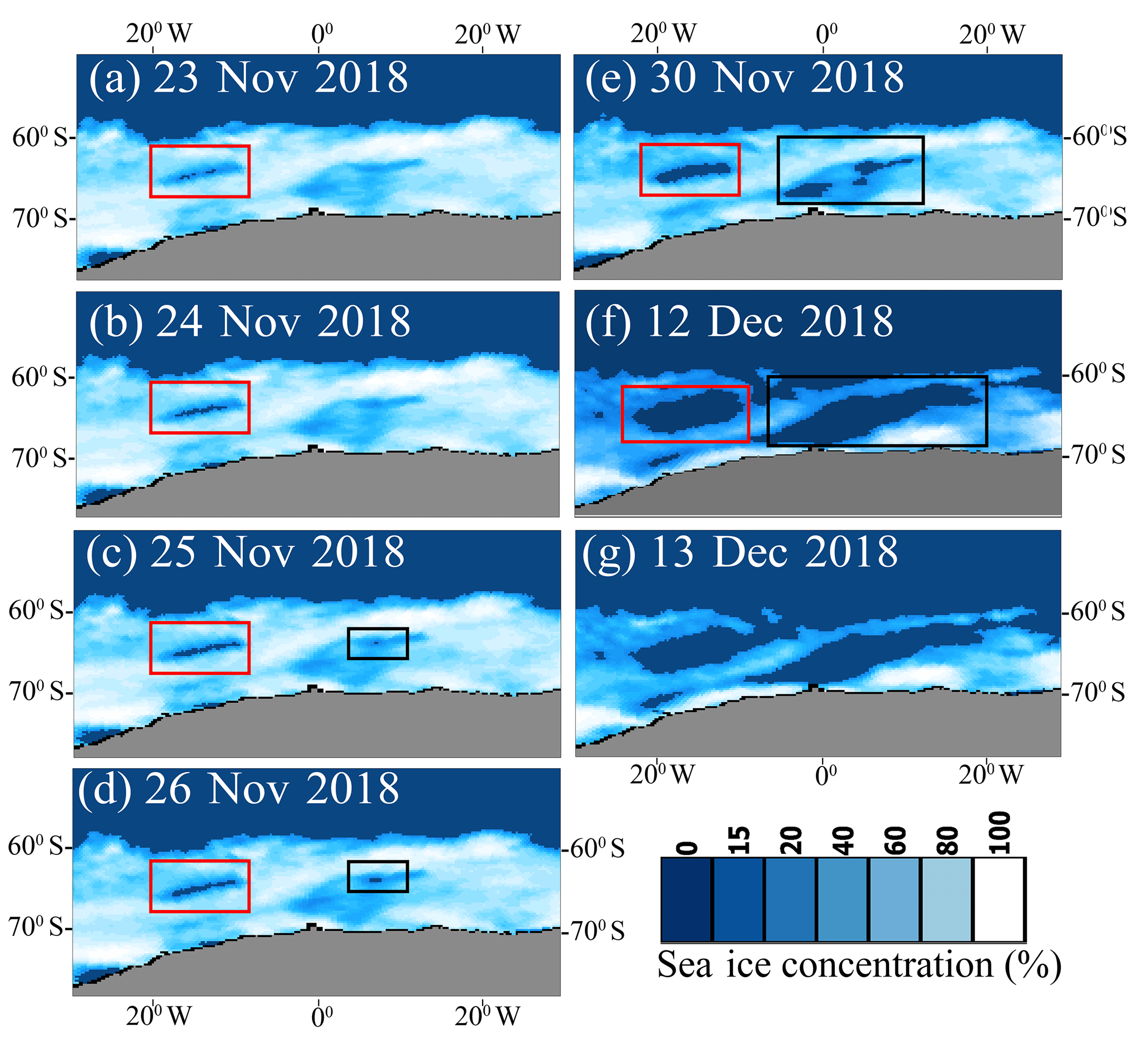
Figure 10 The Special Sensor Microwave Imager/Sounder (SSMIS) shows the reappearance of the Weddell Sea (red rectangle) and Maud Rise (black rectangle) polynyas from 23 November 2018 to 12 December 2018. The polynya disappeared on 13 December 2018.

Further, Argo data were utilized to find the linkage between the observed bloom and the ocean pCO₂ conditions. Analysis of Argo data indicated low pCO₂ values that reached as low as 372.8 µatm (Fig. 5d), corresponding to the occurrence of bloom during October–November 2017 (Fig. 5a). The pCO₂ values declined during the occurrence of bloom in comparison with the period of non-bloom conditions in August–September 2017, 2015, and 2016 (Fig.5). The coefficient of correlation (r) between the pCO₂ and chl a was −0.56 (p<0.01) during August–September 2017 (Fig. 8a). The relationship improved ($r=-\mathrm{0.82}$, p<0.01) and the spatial pattern closely matched during the bloom conditions in October–November 2017 (Figs. 8b, 5a–d). The best relationship was observed between the pCO₂ and chl a when the data were log transformed ($r=-\mathrm{0.94}$, p<0.01). The observed low pCO₂ values in the polynya were likely due to the presence of chl a bloom with high NPP, which has the potential to drive CO₂ fluxes from the atmosphere to the ocean after forming a pressure gradient. This biological pumping process in the polynya could play an important role in lowering the atmospheric CO₂ through transferring atmospheric CO₂ to the ocean and subsequently into the ocean sediments. However, it is important to mention that the air–sea exchange of CO₂ is driven by the pCO₂ gradient, solubility of CO₂ in the seawater (function of ocean temperature and salinity), and gas transfer velocity (function of wind speed and SST) (Williams et al., 2017). Follow-up research is required in the future to quantify the contribution from physical and biological processes in the air–sea exchange of CO₂ in the MR polynya and its likely role in regulating the global climate (Gordon and Comiso, 1988; Li et al., 2016).

4 Summary and conclusion

In this article, we have shown that the phytoplankton bloom occurred on the MR seamount during the appearance of the polynya in spring 2017. Analysis of multi-sensor satellite data from CZCS, SeaWiFS, MODIS, and VIIRS indicated that the bloom appeared for the first time in the satellite records since 1978. Since there is no previous report of its occurrence in the MR polynya, we have examined additional data from the Argo float for firm evidence. The ARGO float located at the northwestern edge of the polynya provided evidence of bloom conditions from October to November 2017 compared to the preceding years of 2015 and 2016 when the sea ice was covered at the surface with low chl a. We find that the combined influence of seamount and physical processes is responsible for the formation of the observed bloom. The presence of a seamount on the MR leads to uplift of thermocline and nutrient-enriched deep water that could fertilize the upper ocean through the upwelling process. During the austral winter and spring 2017, the supply of nutrients to the upper ocean arises through Ekman upwelling driven by a large cyclonic ocean eddy and persistent negative wind stress curl. Even though the Ekman upwelling was evident in September 2017, the bloom did not appear in the polynya due to prevailing low irradiance as expected in an austral winter. However, the bloom appeared in austral spring (October–November 2017) under the influence of Ekman upwelling and improved light conditions that favored the phytoplankton photosynthesis and growth. Low pCO₂ conditions prevailed in the polynya due to the presence of chl a bloom with high NPP that can lead to sinking of atmospheric CO₂ fluxes into the ocean. The observed phytoplankton bloom reported in this article has large importance for the HNLC status of the SO.

Studies have shown intensification of polar cyclone activities due to the poleward shifting of the extratropical cyclone track in the background of a warming climate condition (Francis et al., 2019; Fyfe, 2003). As the polar cyclones are known to trigger the occurrence of polynyas (Francis et al., 2019; Jena et al., 2019; Turner et al., 2017) (through advection of moist, warm air from the extratropics, and sea ice divergence), the frequency of polynya events is likely to increase in the future (including over the MR) under a warming climate condition. The likelihood for the occurrence of the polynya is quite high with a background of anomalous upper ocean warming and sea ice loss, similar to the events that occurred in the Antarctic sea ice from 2016 to 2019 (Fig. 9). Indeed, the Weddell Sea and MR polynya reappeared in 23 November 2018 and lasted till 12 December 2018 as observed from SSMIS (Fig. 10). With the frequent reoccurrence of polynyas on the MR, the associated physical processes could possibly modify the region into a productive environment and likely have an impact on the regional ecosystem and carbon cycle. The occurrence of polynya and phytoplankton blooms in the MR may turn it into a potential sink of atmospheric CO₂ through biological pumping and can be a major source of carbon and energy for the regional food web. The spatial dimension of the bloom in a polynya might be small; however, it is necessary to monitor and understand many important features of the Antarctic marine ecosystem in order to understand its complete role in the global biogeochemical cycle. The study demonstrates how the phytoplankton in the Southern Ocean (specifically over the shallow bathymetric region) would likely respond in the future under a warming climate condition and continued melting of Antarctic sea ice.