the Creative Commons Attribution 4.0 License.
the Creative Commons Attribution 4.0 License.
 | 15 Apr 2020
Unprecedented atmospheric conditions (1948–2019) drive the 2019 exceptional melting season over the Greenland ice sheet
Marco Tedesco
Xavier Fettweis
Understanding the role of atmospheric circulation anomalies on the surface mass balance of the Greenland ice sheet (GrIS) is fundamental for improving estimates of its current and future contributions to sea level rise. Here, we show, using a combination of remote sensing observations, regional climate model outputs, reanalysis data, and artificial neural networks, that unprecedented atmospheric conditions (1948–2019) occurring in the summer of 2019 over Greenland promoted new record or close-to-record values of surface mass balance (SMB), runoff, and snowfall. Specifically, runoff in 2019 ranked second within the 1948–2019 period (after 2012) and first in terms of surface mass balance negative anomaly for the hydrological year 1 September 2018–31 August 2019. The summer of 2019 was characterized by an exceptional persistence of anticyclonic conditions that, in conjunction with low albedo associated with reduced snowfall in summer, enhanced the melt–albedo feedback by promoting the absorption of solar radiation and favored advection of warm, moist air along the western portion of the ice sheet towards the north, where the surface melt has been the highest since 1948. The analysis of the frequency of daily 500 hPa geopotential heights obtained from artificial neural networks shows that the total number of days with the five most frequent atmospheric patterns that characterized the summer of 2019 was 5 standard deviations above the 1981–2010 mean, confirming the exceptional nature of the 2019 season over Greenland.
- Article
(22458 KB) - Full-text XML
- BibTeX
- EndNote


Understanding the role of atmospheric circulation changes in the surface mass balance (SMB) of the Greenland ice sheet (GrIS) is crucial for improving estimates of its current and future contribution to sea level changes and for studying recent mass loss trends in the context of multi-decadal timescales. Atmospheric patterns modulate the GrIS mass balance through snowfall and runoff (e.g., Hanna et al., 2008, 2013, 2016; Tedesco et al., 2011, 2016a, b) as well as radiative forcing and surface turbulent heat fluxes (e.g., clouds and longwave and shortwave radiation). Recent studies (e.g., Hanna et al., 2014; Mattingly et al., 2016; McLeod and Mote, 2016) have focused on linking the observed variability of climate indices such as the North Atlantic Oscillation (NAO; i.e., Hanna et al., 2015) or the Greenland Blocking Index (GBI; Hanna et al., 2018b) to the recent changes in runoff and accumulation over Greenland. Other studies (i.e., Tedesco et al., 2016b) have recently pointed out the increased frequency of persistent anticyclonic conditions favoring atmospheric blocking and explaining most of the recent surface melt increase (Fettweis et al., 2013).
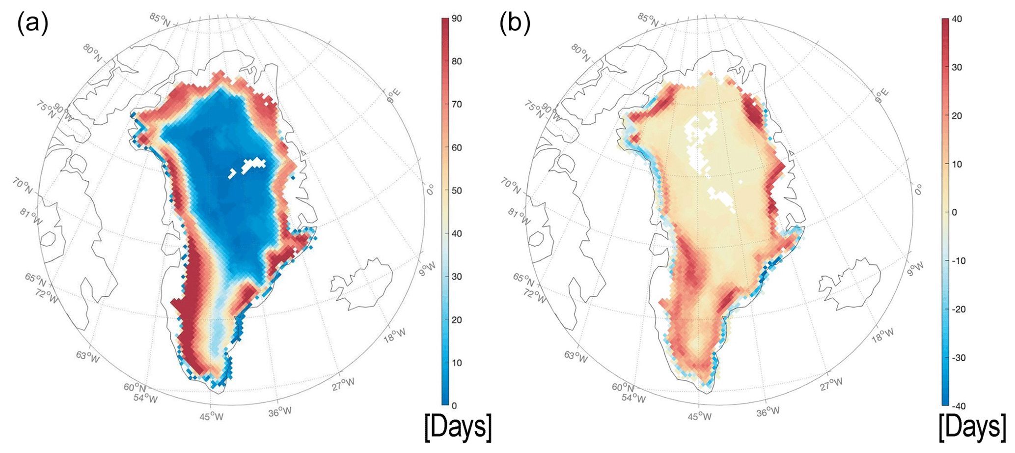
Figure 1(a) Number of days when melting occurred during the 2019 summer (June, July, August, JJA) according to spaceborne passive microwave observations (e.g., Tedesco et al., 2007). (b) Anomaly of the number of melting days with respect to the 1981–2010 baseline period obtained from spaceborne passive microwave data shown in (a).

Figure 2(a) Daily time series of melt extent (expressed as a percentage of the total ice sheet area) during 2019 (black line). The red line indicates the average values for the baseline period 1981–2010. Vertical gray bars indicate the standard deviation of melt extent for the 1981–2010 baseline period. (b) Summer maximum melt extent (as a percentage of the ice sheet surface, blue line, left axis) and melting index (e.g., number of melting days times the area undergoing melting, square kilometers per day, orange line, right axis) obtained from spaceborne passive microwave observations for the period 1979–2019.
In this paper, we report the results of an analysis of SMB and surface energy balance (SEB) components obtained from satellite data and model outputs for the summer of 2019 and their linkages to anomalies in the atmospheric circulation and analyze them within the long-term context (1948–2019). Specifically, we use spaceborne passive microwave data collected between 1979 and 2019 at 19.35 GHz, horizontal polarization, for detecting melting following the approach reported in Tedesco (2007, 2009) and Tedesco et al. (2007). We also use estimates of broadband albedo derived from data collected by the Moderate Resolution Imaging Spectroradiometer (MODIS) for the period 2000–2019 (https://terra.nasa.gov/about/terra-instruments/modis, last access: 31 March 2020). We complement satellite data with the outputs of the Modèle Atmosphérique Régionale (MAR) regional climate model (RCM; Gallée and Schayes, 1994; Gallée, 1997; Lefebre et al., 2003) forced by the National Centers for Environmental Prediction/National Center for Atmospheric Research (NCEP/NCARv1; Kalnay et al., 1996) reanalysis dataset over the period 1948–2019. We lastly make use of self-organizing maps (SOMs; i.e., Kohonen, 2001) to classify pan-Arctic summer 500 hPa geopotential height (GPH) anomalies (1981–2010 baseline period) also obtained from the NCEP/NCAR reanalysis dataset (Kalnay et al., 1996) between 1948 and 2019. The pan-Arctic region is here defined as the portion of the Northern Hemisphere poleward of 60∘ N. We focus on the 500 hPa GPH values because of their strong correlation with SMB quantities and for consistency with other studies using them to compute climate indices, such as the GBI (e.g., Hanna et al., 2016). Moreover, 500 hPa is also a standard height for gauging the effects of jet stream blocking on synoptic weather patterns (e.g., McIlveen, 2010).
2.1 Satellite data
Passive microwave (PMW) brightness temperatures (Tbs) are a crucial tool for studying the evolution of melting over the Greenland and Antarctica ice sheets (e.g., Abdalati and Steffen, 1995; Tedesco, 2007, 2009; Tedesco et al., 2009; Fettweis et al., 2011). The capability of passive microwave sensors to collect useful data during both day- and nighttime and in all-weather conditions provides data at a high temporal resolution (at least daily over most of the Earth), with high latitudes being covered several times during a single day. Since the launch of the Scanning Multichannel Microwave Radiometer (SMMR) in October 1978, Tb data have been available in multiple bands every other day (in the case of SMMR) and daily starting in 1987, with the launch of the Special Sensor Microwave Imager (SSMI). PMW brightness temperature records are the longest available time series and an irreplaceable tool in climatological and hydrological studies, especially for those regions, such as the ice sheets, where in situ observations are lacking and fieldwork is logistically difficult, if not impossible. Specifically, we make use of data distributed by the National Snow and Ice Data Center (NSIDC, https://nsidc.org/, last access: 31 March 2020; https://catalog.data.gov/dataset/near-real-time-dmsp-ssm-i-ssmis-pathfinder-daily-ease-grid-brightness-temperatures-version, last access: 31 March 2020) at a spatial resolution of 25 km at the K band (∼19 GHz), horizontal polarization. Melting is detected following the procedure described in Tedesco (2007, 2009).
We complement PMW data with the MODIS daily surface reflectance product (MOD09GA version 6) and daily snow cover product (MOD10A1 version 6, https://nsidc.org/sites/nsidc.org/files/files/MODIS-snow-user-guide-C6.pdf, last access: 31 March 2020). The MOD10A1 data include broadband albedo estimated based on the MOD09GA product. We used the version 6 data in view of its improvement in sensor calibration, cloud detection, and aerosol retrieval and correction relative to version 5 (e.g., Casey et al., 2017). Version 6 data are optimal for assessing temporal variability of surface albedo as they are corrected for sensor degradation issues impacting earlier versions (Casey et al., 2017). The spatial resolution of the MODIS datasets is 500 m. We use the cloud mask in the MOD10A1 data to exclude clouds.
2.2 The MAR regional climate model
The regional climate model MAR (Fettweis et al., 2017) combines atmospheric modeling (Gallée and Schayes, 1994) with the Soil Ice Snow Vegetation Atmosphere Transfer Scheme (De Ridder and Gallée, 1998) and has been extensively evaluated and used to simulate surface energy balance and mass balance processes over GrIS (e.g., Fettweis, 2007; Fettweis et al., 2011). In this study, we use version 3.10 of MAR, at a horizontal spatial resolution of 20 km as in Fettweis et al. (2017) and 6 h temporal resolution forced with the NCEP/NCARv1 reanalysis (Kalnay et al., 1996). Outputs generated at sub-daily temporal resolution are, then, averaged to obtain daily values. We refer to Fettweis et al. (2017) for the evaluation of this NCEP/NCARv1 forced simulation and to Delhasse et al. (2020) for the list of improvements made since MARv3.5 used in Fettweis et al. (2017).
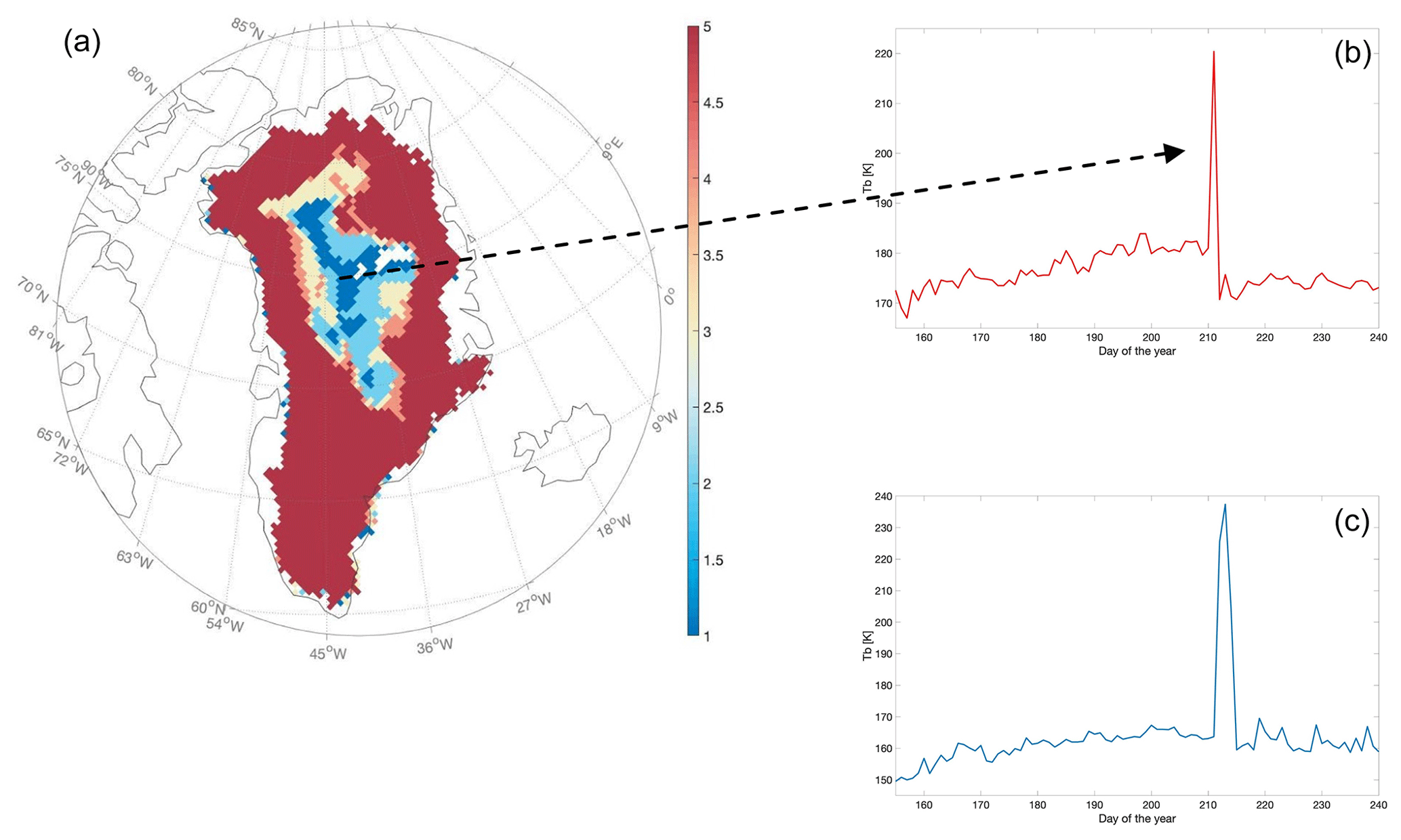
Figure 3(a) Number of melting days in 2019 obtained from spaceborne passive microwave observations. The data are the same as those in Fig. 1 but the range has been reduced between 1 and 4 d to highlight melting occurring in the interior at high elevations. (b, c) Daily time series of spaceborne microwave brightness temperatures for the two selected points indicated by the tail of the arrow.
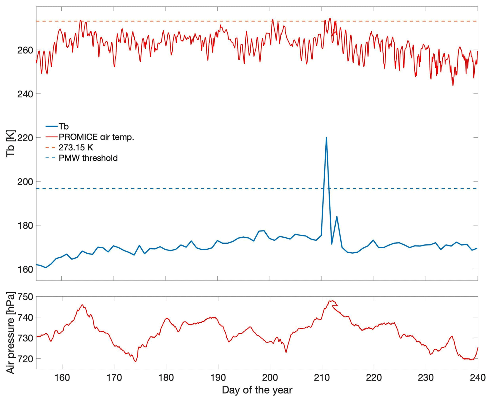
Figure 4Time series of daily air temperature (top red line) recorded at the EGP PROMICE station (75.6247∘ N, 35.9748∘ W, 2660 m a.s.l.) together with time series of spaceborne brightness temperatures at 19.35 GHz recorded over the pixel containing the location of the EGP station (blue line) together with air pressure (hPa) recorded at the same station (bottom red line). The dashed orange line represents the 273.15 K values, and the blue dashed line represents the threshold on Tb above which melting is considered to occur.
2.3 NCEP/NCAR reanalysis data and the Greenland Blocking Index (GBI)
We use geopotential heights at 500 hPa obtained from the NCEP/NCAR reanalysis dataset, consisting of globally gridded data that incorporate observations and outputs from a numerical weather prediction model from 1948 to present (Kalnay et al., 1996). We also use the so-called Greenland Blocking Index (GBI), defined as the mean 500 hPa geopotential height over the area bounded by the coordinates 60–80∘ N, 20–80∘ W (e.g., Hanna et al., 2015, 2018a). Positive GBI conditions are generally associated with surface high pressure “blocking” anomalies over the Greenland region (Hanna et al., 2016). There is also a strong and significant anti-correlation between Greenland blocking and the North Atlantic Oscillation (NAO, the first mode of atmospheric surface pressure variation over the North Atlantic), with Greenland blocking typically linked to a southward deflection of the jet stream (Hanna et al., 2015, 2018b; Tedesco et al., 2016b). Here, we use a recent reconstruction of GBI from 1851 to 2019 (Hanna et al., 2018a) that combines data from the 20CRV2c Reanalysis (Compo et al., 2011) with newer (1948–2015) data from the NCEP/NCAR reanalysis (Kalnay et al., 1996).
Melt duration in 2019 (Fig. 1a) estimated from PMW data exceeded the long-term (1981–2010) mean by up to 40 d along the west portion of the ice sheet where dark, bare ice is exposed (Fig. 1b). Over the rest of the ice sheet, the anomaly of the number of melting days during the summer of 2019 from PMW data was around 20 d. Negative anomalies were rare and geographically concentrated over a small area in the southern portion of the ice sheet. Surface melting in 2019 started relatively early, around mid-April (Fig. 2a, day of the year, DOY 105), and exceeded the 1981–2010 mean for ∼82 % of the days during the period 1 June–31 August 2019 (DOY 152–244). A measure that is commonly used for quantifying melting from passive microwave observations is the so-called melting index (MI), defined as the number of melting days times the area undergoing melting and being a measure of the intensity of surface melting (i.e., Tedesco, 2007). In 2019, the MI ranked third, after 2012 and 2010. When looking at the different summer months separately, the MI values in 2019 ranked fifth in June, seventh in July, and ninth in August. The 2019 updated trends for MI and melt extent (here defined as the area subject to at least 1 d of melting) are, respectively, 78.836 km2 per decade (p≪0.01, MI) and 7.66 % per decade (p≪0.01; trend is here expressed as a percentage of the total area of the ice sheet). The maximum daily melt extent was reached on 31 July 2019, covering ∼73 % of the ice sheet surface. In comparison, the average daily maximum extent from PMW data for the same day for the 1981–2010 period is 39.8 %. Notably, the total area that at any time underwent melting was 95.8 % of the total ice sheet in 2019 (Fig. 2b), compared with the 1981–2010 averaged value of 64.3 %. Indeed, the persistency of the atmospheric conditions at the end of July that were responsible for promoting melting over 73 % of the ice sheet in a single day (31 July 2019) extended melting during the next few days over regions that were not originally involved in the melting on 31 July, with cumulative melt extent for the 3 d period (31 July–2 August) reaching up to ∼97 % of the ice sheet surface. We note that a similar value for the maximum melt extent was reached in 2012, though in this case it did happen in 1 d. As in 2019, the exceptional melt in 2012 was associated with the advection of very warm and wet air masses coming from the south and promoting the presence of liquid water clouds promoting surface melt in the dry snow zone (e.g., Tedesco et al., 2016b). However, in 2019, the air mass came from the east after promoting an exceptional heat wave in Europe, being warmer and drier than the air mass in 2012. Moreover, by crossing the relatively cold Atlantic Ocean from Scandinavia, in 2019 the lower atmospheric layers cooled down, increasing the stability of the air mass and then limiting the formation of liquid water clouds compared to July 2012, explaining why the melt extent was lower during this 2019 big melt event than in July 2012 while the temperature anomaly was higher in the free atmosphere in 2019 than in 2012.
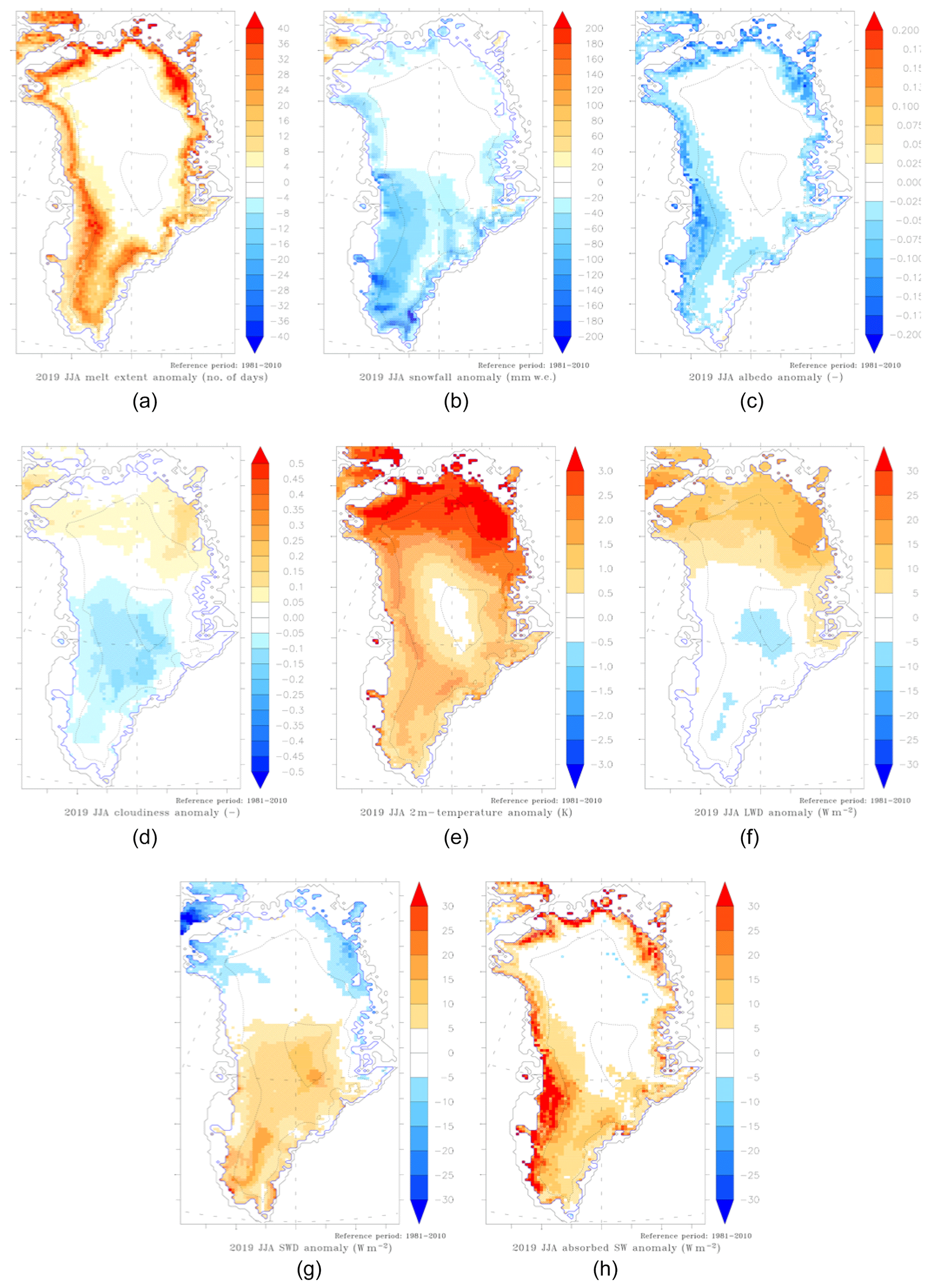
Figure 5Spatial distribution of the anomaly of the (a) number of melting days, (b) snowfall, (c) albedo, (d) cloudiness, (e) 2 m temperature, (f) longwave downwelling radiation, (g) shortwave downwelling radiation, and (h) shortwave radiation absorbed obtained from the MAR model (1981–2010 baseline) forced by the reanalysis NCEP/NCARv1.

Figure 6Time series of 1949–2019 annual (1 September 2018–31 August 2019) SMB (dark blue), snowfall (red), and runoff (yellow) values simulated by MAR over the whole Greenland ice sheet.
We investigated the possibility that the sporadic melting detected at high elevations could have been due to a malfunctioning of the sensor or other issues related to data quality. Figure 3a shows a map of the number of melting days constrained to values ranging between 1 and 4 d to highlight those areas where melting occurred for a few days at high elevations. In the figure, we also show the time series of brightness temperatures for those pixels where melting occurred for only 1 d (Fig. 3b) or for 2 d (Fig. 3c). The sharp, sudden increase in brightness temperatures is not associated with data quality issues but rather with the insurgence of melting in both cases. Melting at high elevations is also confirmed from the analysis of in situ data. For example, Fig. 4a shows air temperature (2 m) recorded at the EGP PROMICE station (75.6247∘ N, 35.9748∘ W, 2660 m a.s.l., https://www.promice.dk/WeatherStations.html, last access: 31 March 2020) together with time series of spaceborne Tbs at 19.35 GHz, horizontal polarization, recorded over the pixel containing the location of the EGP station (blue line). Air (2 m) pressure (hPa) recorded at the same station is also reported as a red line in the bottom plot. The figure shows that air temperature exceeded the value of 0 ∘C when Tb values sharply increased from ∼170 to ∼220 K. Concurrently, surface air pressure reached peak values of ∼749 hPa at EGP, likely as a consequence of the persistent anticyclonic conditions occurring during that period. We also note that air temperature exceeded the melting point at least twice in 2019 at the EGP station in addition to 31 July, according to the in situ data: the first time on day 163 (12 June) and the second time on day 201 (19 July). In both cases, however, the passive microwave data did not detect the presence of liquid water. This might be a consequence of the fact that air temperature can be exceeding the melting point when snow temperature is not and that the second event, when air temperatures exceed the melting point, was characterized by relatively low pressure. This suggests that the radiative forcing associated with the incoming solar radiation might not have been as strong as in the case of the end of July.
The spatial distribution of the anomaly of the number of melting days obtained from PMW observations is consistent with the one obtained from the MAR regional model, as shown in Fig. 5a. Here, we consider those cases when the integrated liquid water content in the top meter of the snowpack reaches or exceeds 1 mm w.e., following Fettweis et al. (2007). Meltwater runoff in JJA 2019 simulated by MAR and integrated over the whole ice sheet ranked second (consistently with the MI values obtained from the PMW data), reaching a total of 560 Gt in 2019 against an average value of 300±85 Gt yr−1 for the 1981–2010 period. As a reference, the value of runoff simulated by MAR for the JJA 2012 period (when the record was established) was 610 Gt. Despite ranking second in terms of surface runoff, September 2018–August 2019 (used to define the mass balance “year”) ranks first in terms of integrated SMB negative anomaly simulated by MAR, with a total surface mass loss anomaly of ∼320 Gt yr−1 with respect to the 1981–2010 SMB average, breaking the previous record established in 2011–2012 of ∼310 Gt yr−1 (Fig. 6, blue bars), though by only 10 Gt yr−1. It is however important to note that such a difference is below the uncertainty of the MAR model estimated to be 10 % of the mean SMB.
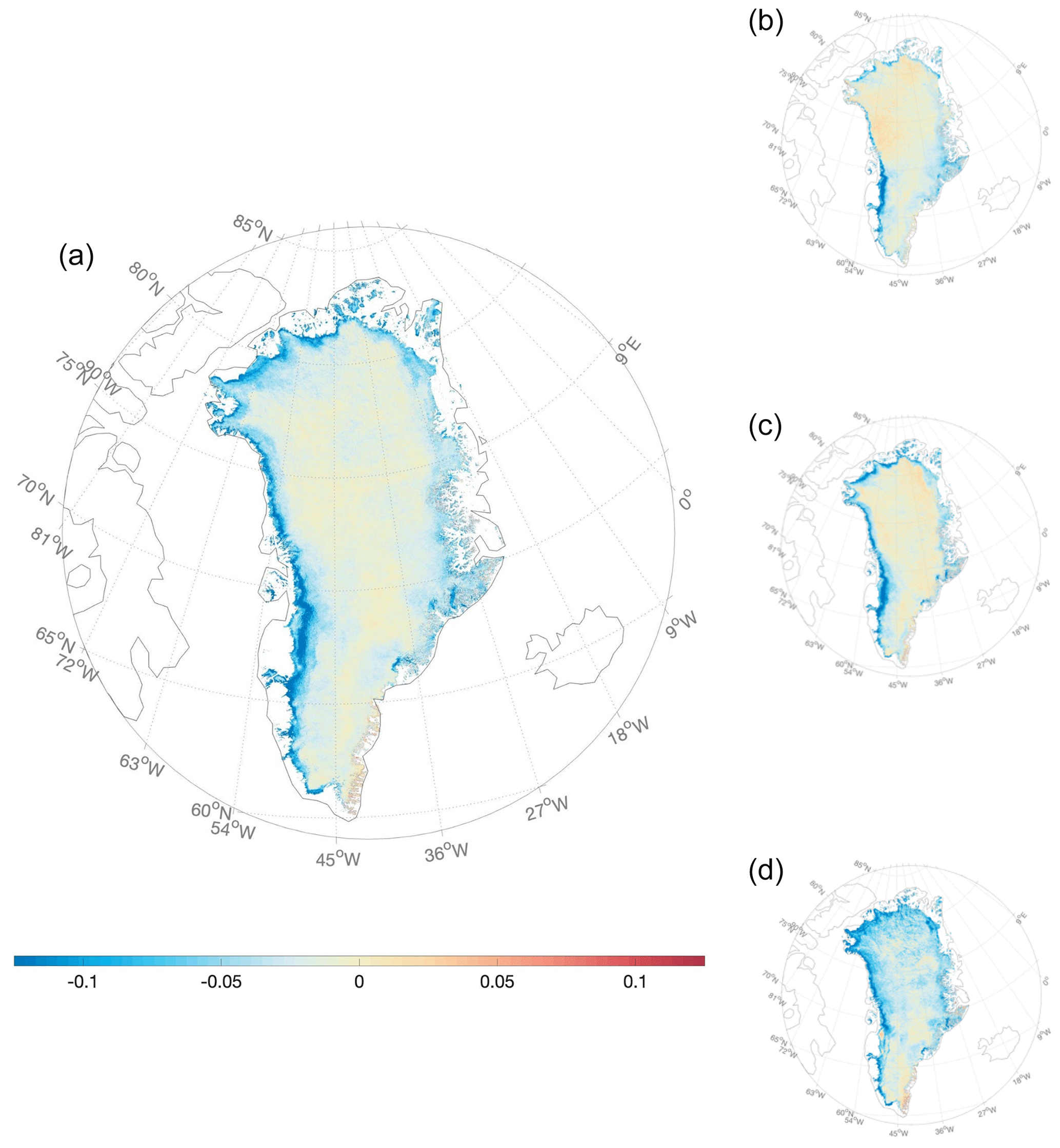
Figure 7MODIS 2019 broadband albedo values anomalies (2000–2010 baseline) for (a) summer, (b) June, (c) July, and (d) August.
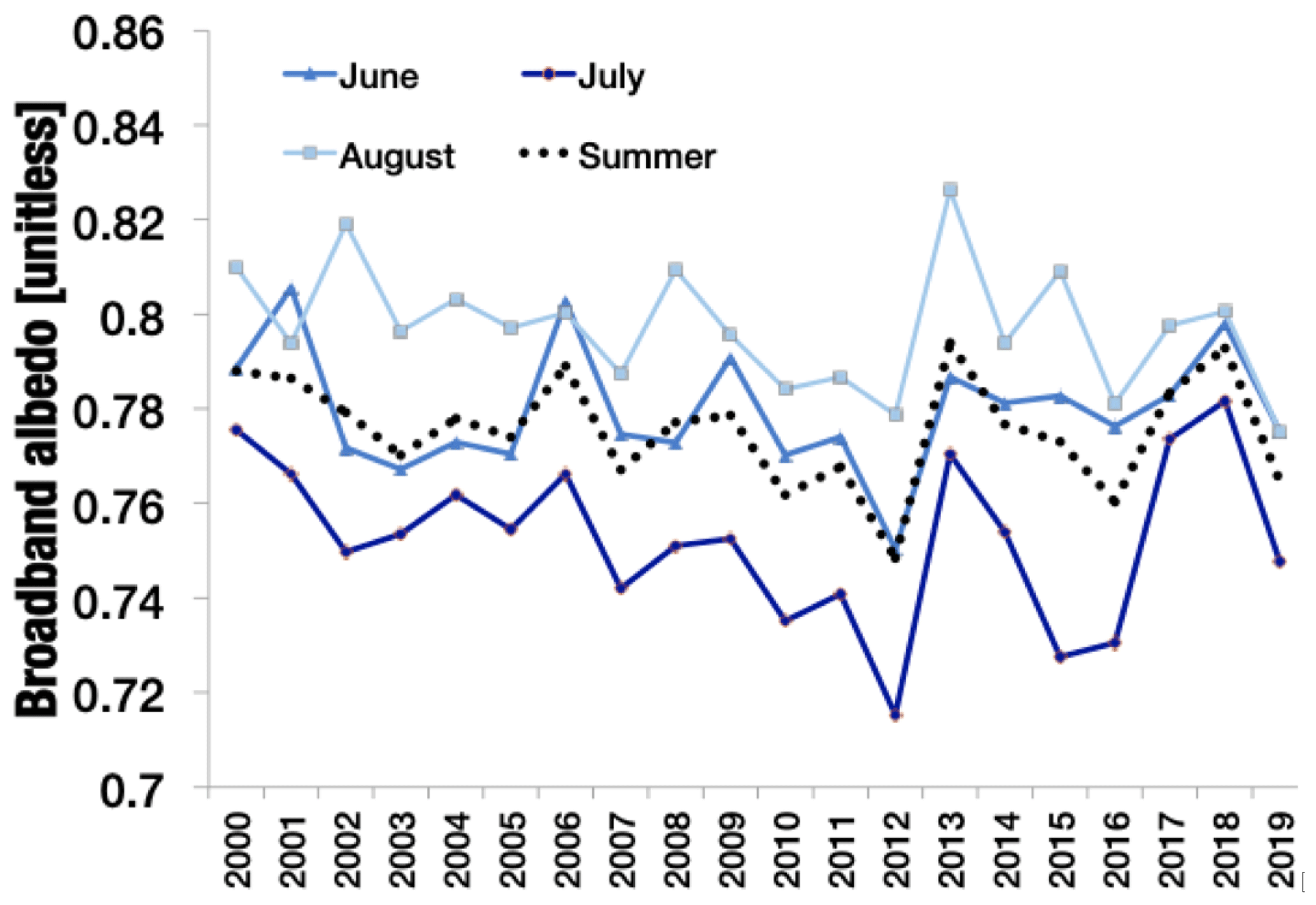
Figure 8Time series of MODIS 2019 broadband albedo values for summer (dark dotted line), June (medium blue line with triangles) July (dark blue line with disks), and August (light blue line with squares).
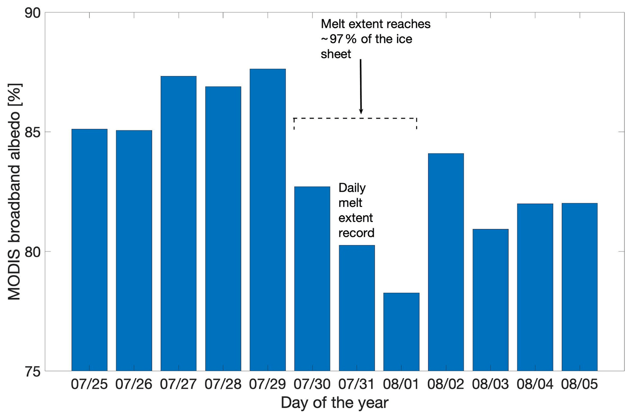
Figure 9Time series of values of MODIS broadband albedo for the pixel whose brightness temperature is shown in Fig. 3b.
The SMB negative anomaly in 2018–2019 is larger than that in 2011–2012 mainly because the 2018–2019 snowfall negative anomaly ( Gt) is larger in magnitude than the one that occurred during the 2011–2012 SMB year ( Gt), with large negative summer snowfall anomalies in 2019 occurring along the southern and western portions of the ice sheet (Fig. 5b). The early melt onset and the negative snowfall anomaly promoted the exposure of bare ice prematurely, hence further enhancing melting and runoff through the melt–albedo positive feedback mechanism (i.e., Tedesco et al., 2016b). This is evident from the analysis of summer broadband albedo simulated by MAR (Fig. 5c), showing negative anomalies down to −0.2 along the western portion of the ice sheet. These results are also confirmed by albedo estimates obtained from MODIS (Fig. 7a), indicating a large, negative albedo anomaly occurring along the west coast where bare ice is exposed. Specifically, summer MODIS albedo ranked fourth (Fig. 8) within the 2000–2019 MODIS period, with −1.45 standard deviations (σ) below the mean (2000–2010 baseline period). The summer of 2019 precedes the ones of 2010 (−1.79σ), 2016 (−1.95σ), and 2012 (−3.33σ) in terms of MODIS albedo. When considering the summer months separately, June and July 2019 ranked, respectively, 10th (June) and seventh (July). A new record was, nevertheless, established in August 2019, with the absolute value averaged over the whole ice sheet reaching 77.51 % (−2.39σ) in 2019, followed by 2012 (77.86 %, −2.05σ) and 2016 (78.1 %, −1.81σ). The updated trend over 2000–2019 for summer broadband albedo is −0.4 % per decade, though it is not statistically significant (R2=0.04). Similarly, the trends for June (−0.1 %), July (−0.6 %), and August (−0.7 %) are also not statistically significant.
The analysis of the maps of the monthly averaged albedo (Fig. 7b through d) indicates that, as mentioned above, negative albedo anomalies occurred along the western portion of the ice sheet in June and July but, during the same period, albedo was within the average over most of the rest of the ice sheet. In June, only 23 % of the ice sheet surface was showing positive albedo anomalies. The value for July was 25 %, to be reduced to only 6 % in August. During this month, the negative albedo anomalies in the south are confined along a relatively small portion of the west margin of the ice sheet, but they extend further inland, reaching high elevations in the northern regions (Fig. 7c). The presence of negative albedo anomalies in August at higher elevations is consistent with the sporadic melting that occurred over the same region at the end of July and beginning of August 2019 (Fig. 3). The impact of such an event is, indeed, observable in the albedo changes of the pixel that underwent melting for 2 d at the end of July (Fig. 9, the same as the one whose Tb values are shown in Fig. 3b), showing a reduction from 87.4 % to 77.8 % due to the increase in grain size associated with the melting and refreezing cycle.
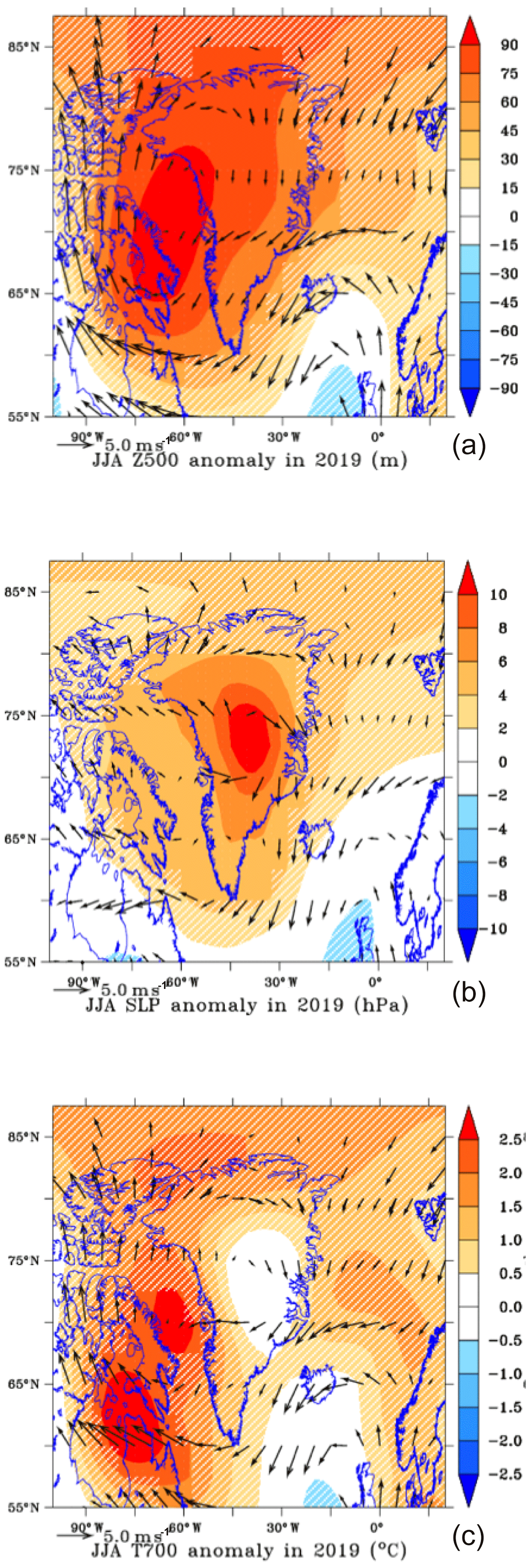
Figure 10(a) JJA 2019 averaged geopotential height anomalies at 500 hPa (Z500 in meters, baseline period 1981–2010) from the NCEP/NCARv1 reanalysis. Anomalies below 2 times the interannual variability (i.e., not statistically significant) are hatched. (b) Same as (a) but for the sea level pressure (hPa) and for (c) JJA temperature at 700 hPa (∘C). In each panel, arrows represent the anomaly of JJA winds at (a) 500 hPa, (b) 10 m, and (c) 700 hPa.

Figure 11Absolute values of the temperature at (a, d) 700 hPa (T700) and (b, e) 500 hPa (T500) and (c, f) mean specific humidity over 700–500 hPa from NCEP/NCARv1 reanalysis on 12 July 2012 (a, b, c) and on 31 July 2019 (d, e, f).
A major driver of the exceptional melting season in 2019 was the persistency of high-pressure systems over the GrIS that promoted an increase in the absorbed solar radiation as well as the flow of warm, moist air along the western portion of the ice sheet towards the north of the ice sheet. The anticyclonic conditions were also responsible for reduced cloudiness in the south and consequent below-average summer snowfall and albedo in this area. Similarly to 2012, anticyclonic conditions dominated summertime (Fig. 10a). The anomaly also occurred at the surface (Fig. 10b), suggesting that the pressure anomaly in the mid-troposphere was driven by atmospheric circulation rather than by the warming of the free atmosphere below 500 hPa levels. The anticyclonic conditions also promoted the advection of warm air that reached the northern portion of the ice sheet, explaining why the highest temperature anomaly at 700 hPa occurs in this area (Fig. 10c). As a reference, Fig. 11 shows the absolute values of the temperature at 700 hPa (T700) and 500 hPa (T500) and the mean specific humidity over 700–500 hPa from NCEP/NCARv1 reanalysis on 12 July 2012 and on 31 July 2019. While the temperature anomalies were higher in 2019 with respect to the climatology of mid-July or of the end of July, the absolute values were higher in 2012 than in 2019. In addition, the humidity content was also higher in 2012 than in 2019 over the ice sheet, showing the important role of liquid clouds in the 2012 extreme melt event (Bennartz et al., 2013). These differences in temperature and humidity pattern explain why the 2012 highest melt event was more extreme than the 2019 one. Over the center of the ice sheet, surface temperature was close to the 1981–2010 average, suggesting a larger role of the radiative forcing than the thermal one. The mean summer sea level pressure (SLP) averaged over the 60–80∘ N, 20–80∘ W region (i.e., the same area used to compute GBI; Hanna et al., 2016) reached a breaking record value of 1016 hPa vs. a 1981–2010 summer average of 1010±2 hPa. Also, the summer averaged 500 hPa geopotential heights, integrated over the same area, set a new record of 5567 m, against a 1981–2010 average of 5497±25 m (Fig. 12a). We computed the persistency of anticyclonic conditions, defined here as the number of days when the daily mean SLP averaged over the Greenland ice sheet exceeds 1013 hPa (the common value of the standard pressure), and we found that during the summer of 2019 such conditions existed for 63 of the 92 summer days (68 % of the summer). In perspective, the average number of days with the same conditions during the period 1981–2010 was 28±12 d.
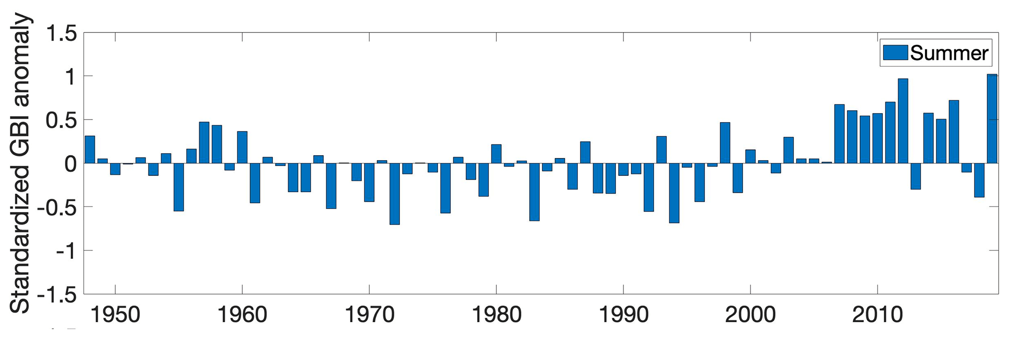
Figure 12Standardized (1981–2010) (a) summer (JJA) averaged GBI values for the period 1948–2019.
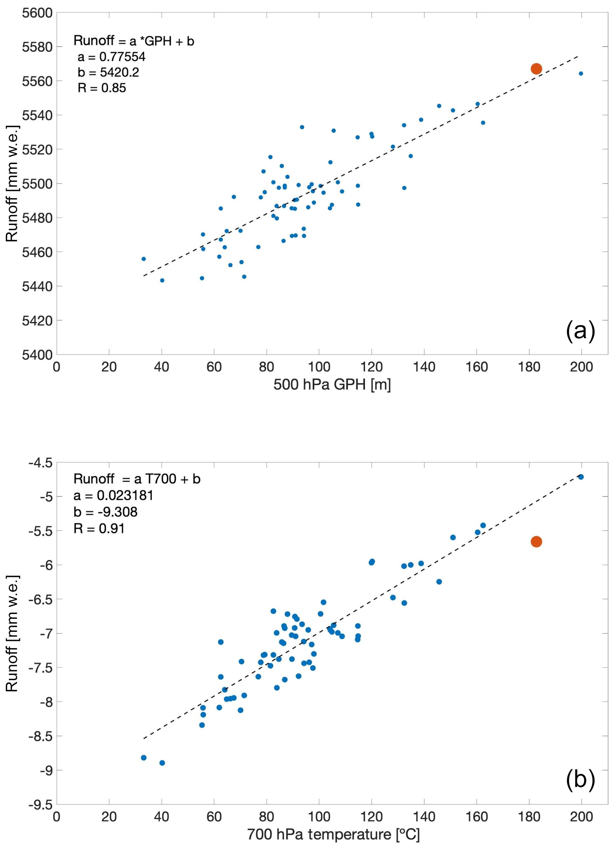
Figure 13Scatterplot between runoff (mm w.e.) and (a) 500 hPa GPH (m) and (b) 700 hPa temperature (∘C). Red disks show 2019 values in both plots. The coefficient of a linear regression analysis are reported within each plot, together with the coefficient of determination R.
The anticyclonic conditions that characterized the summer of 2019 promoted negative cloudiness anomalies over the southern portion of the ice sheet and positive ones over the northern region (Fig. 5d), pointing to the important role of clouds in enhancing melting in this area (i.e., Hofer et al., 2017). In the north, the exceptional persistence of a high-pressure system centered near Summit over the whole of the 2019 summer (Fig. 11b) favored advection of warm and wet air along the west side of Greenland towards the north, promoting higher-than-average surface temperatures (Fig. 5e) and positive anomalies of longwave downwelling radiation (Fig. 5f). In the southwest, dry and sunny conditions dominated. This promoted positive anomalies of the incoming shortwave radiation (Fig. 5g) which, in turn, when combined with the relatively low albedo (due to reduced summer snowfall) promoted positive anomalies of the absorbed shortwave radiation (Fig. 5h) higher than 30 W m−2. Such drier conditions also allowed temperatures to decrease during nighttime, explaining why the temperature anomaly was not playing a larger role over these regions. Integrated over the whole ice sheet, the anomalies of shortwave and longwave downwelling radiation were not significant, but, as a result of a quasi permanence of exposure of low-albedo zones, the anomaly of absorbed shortwave radiation was the highest since 1948, with an anomaly integrated over the whole ice sheet of 7.9 W m−2, 4 times the 1981–2010 standard deviation (inter-annual variability) of 1.9 W m−2. The strong relationship between runoff and atmospheric conditions is also apparent in Fig. 13, where scatterplots of runoff with 500 hPa GPH summer mean anomalies (Fig. 13a) and with 700 hPa temperature (Fig. 13b) are shown, together with the coefficients of the linear regression between runoff and the two atmospheric quantities. Reinforcing the idea that radiative forcing played a large role with respect to thermal forcing, the summer of 2019 (marked in the two panels with a large, orange circle) is beyond 2 standard deviations from the mean in the case of the 700 hPa temperature where it falls closely to the regression line in the case of the 500 hPa GPH.
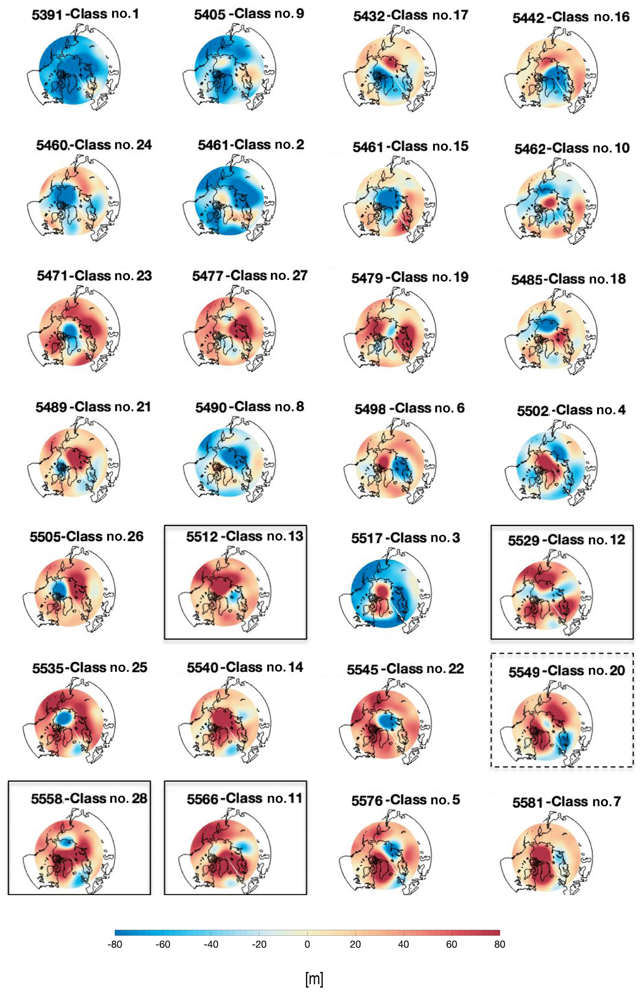
Figure 14Mean 500 hPa GPH anomalies for the 28 classes identified by the SOM using the NCEP/NCAR reanalysis data for the period 1948–2019 ordered from the lowest to the highest mean GBI values computed using those days when the classes were occurring.
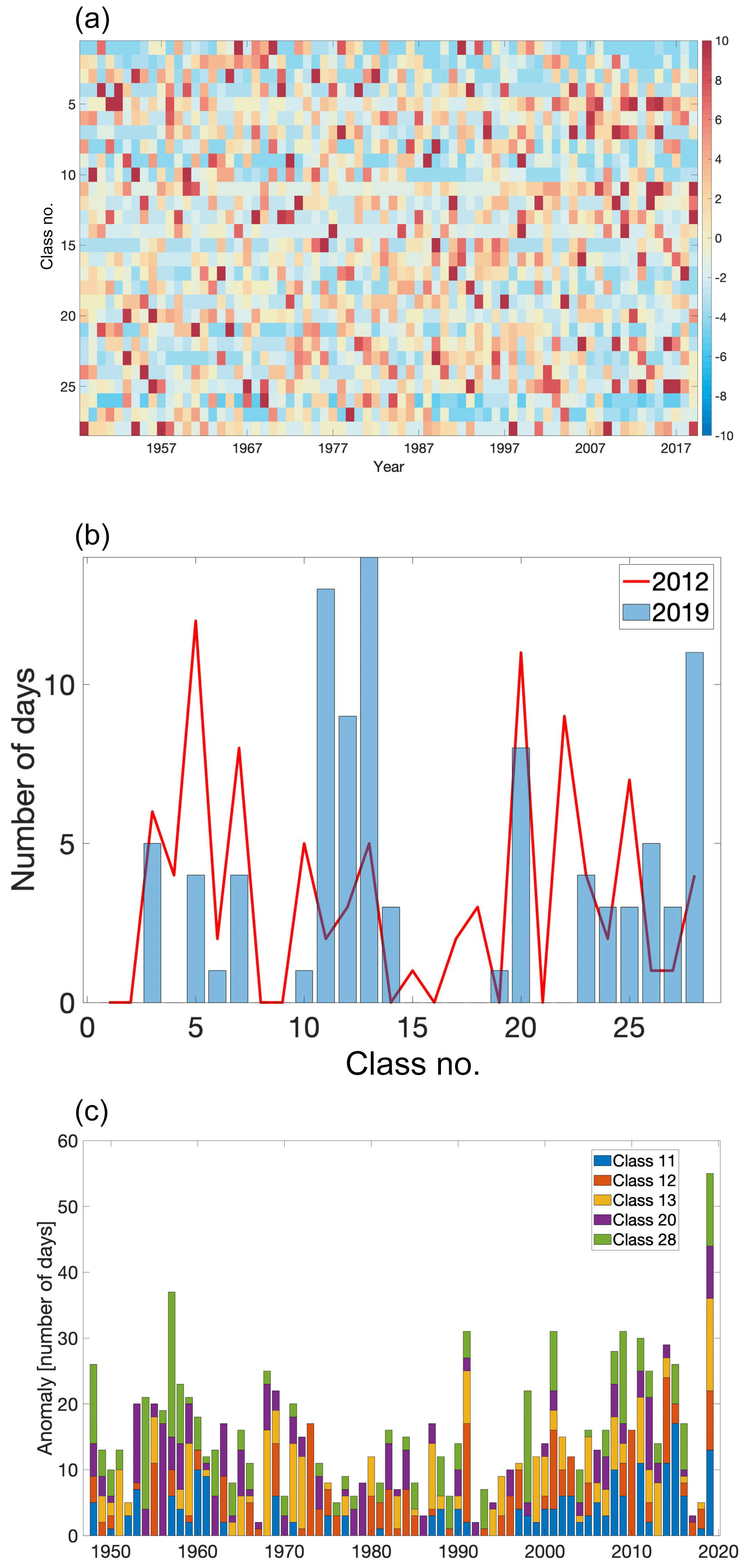
Figure 15(a) Anomaly of the number of days (1981–2010 baseline) of the occurrence of each of the 28 classes identified through the SOM analysis for the years 1948–2019. (b) Number of days when the 28 identified classes (x axis) occur during the summers of 2012 (red line) and 2019 (blue bars). (c) Anomaly of the number of days for class nos. 11, 12, 13, 20, and 28 for the period 1948–2019.
To further understand the role of the atmosphere in the 2019 SMB record and the linkages between atmospheric circulation and SMB, we classified summer (JJA) daily 500 hPa GPH anomalies between 1948 and 2019 into a set number of classes to study how the frequency of such classes has changed over the past decades and how the 2019 summer positioned itself within the 1948–2019 record. We focus on the 500 hPa GPH because of its strong correlation with the surface melt (Fettweis et al., 2011b) and because it is a standard height for gauging the effects of jet stream blocking on synoptic weather patterns (e.g., McIlveen, 2010). We classify the daily 500 hPa GPH anomalies by means of self-organizing maps (SOMs), artificial neural network algorithms that use unsupervised classification to perform nonlinear mapping of high-dimensional datasets (Kohonen, 2001). Initially, a set number of nodes is created (set by the user), and the nodes are randomly filled with the GPH anomalies' daily fields. During the training phase of the SOMs, each of the daily 500 hPa GPH fields is reallocated to one of the classes depending on the Euclidean distance of the new element from the existing SOM nodes. Once trained, the SOM network is interrogated by providing the daily 500 hPa GPH anomaly fields (1981–2010 baseline) and obtaining the corresponding class to which that particular atmospheric field belongs. From here, it is possible to calculate the frequency of occurrence of the classes of the atmospheric circulation patterns to provide insight into possible temporal changes associated with the identified classes and their relationship with SEB and SMB quantities. The number of nodes, which also corresponds to the number of classes in which the atmospheric patterns are classified (Kohonen, 2001), is defined by the user: using fewer nodes allows the user to include a broader range of circulation patterns within the same class but it decreases the amount of variability captured by the SOMs, while increasing the number of node results in classes that are less frequent and more closely resemble each other. Based on previous work (e.g., Mioduszewski et al., 2016) and following Kohonen (2011), we selected a total number of 28 classes. Figure 14 shows the 28 nodes identified through the SOM analysis ordered according to the mean GPH values computed over the same area where GBI is calculated. For each node, the position of each class in the original grid is reported (shown as class no.) together with the mean 500 hPa GPH value. The maps in Fig. 14 are obtained by averaging the 500 hPa GPH values over those days when the specific node was occurring according to the SOM classification. For the reader's convenience, in Fig. 15a we show the anomaly of the summer frequency of occurrence of each class (y axis) for the years 1949 through 2019 (x axis) with respect to the 1981–2010 period. Further, in Fig. 15b we show the number of days occurring in 2019 (blue bars) and 2012 (red line) for the different classes (x axis). We selected 2012 and 2019 because of the enhanced surface melting that characterized both summers. We note that the atmospheric patterns characterizing the two summers show differences and similarities. Both summers, indeed, had a high number of days when class no. 20 (highlighted with a rectangle with dashed contours in Fig. 14) occurred (up to ∼10 d in 2019). This class is characterized by large positive 500 hPa GPH anomalies (above 80 m) over Greenland and the Canadian archipelago, negative anomalies over Scandinavia, and large positive anomalies over Siberia. Differently from 2012, however, class nos. 11, 12, 13, and 28 were persistently present in 2019 (highlighted in Fig. 14 with rectangle with a continuous line). Class nos. 12 and 13 show relatively low 500 hPa GPH anomalies over Greenland but strong positive anomalies over the Arctic Ocean (class no. 13) and the Canadian archipelago, eastern Siberia, and Scandinavia (class no. 12). Class nos. 11 and 28 show large positive anomalies over Greenland reaching both the Canadian archipelago and northern Europe and relatively high positive 500 hPa GPH anomalies over Siberia and Alaska. Notably, the cumulative number of days identified for class nos. 11, 12, 13, 20, and 28 exceeded 55 d in 2019 (Fig. 15c), being 5.1 standard deviations above the 1981–2010 mean of 14.2 d. This points out, again, the exceptional nature of the atmospheric conditions over Greenland during the summer of 2019. Nevertheless, we observe from Fig. 14b that 2012 also had high persistency in atmospheric patterns, though such patterns belong to different classes than those in 2019. For example, the cumulative number of days for 2012's top five classes is 47, similar in magnitude to the 55 d for 2019's top five classes. Moreover, similarly to 2019, the top five classes in 2012 were all characterized by high GPH anomalies and strong anticyclonic conditions (though different in terms of spatial distribution of the GPH anomalies). In this regard both 2012 and 2019 can be assumed to be exceptional from an atmospheric point of view.
Using a combination of remote sensing observations, regional climate model outputs, reanalysis datasets, and self-organizing maps (SOMs), we have shown that exceptional anticyclonic conditions occurred in the summer of 2019 and promoted new record or close-to-record values of SMB, runoff, and snowfall. Runoff in 2019 was the second highest after 2012, and SMB was the lowest on the record according to MAR forced by NCEP/NCARv1. The exceptional nature of the mass balance components in 2019 was strongly driven by albedo reduction associated with reduced summer snowfall, enhanced absorption of solar radiation, and the flow of warm, moist air along the western portion of the ice sheet. The analysis of the frequency of daily 500 hPa GPH obtained from SOMs shows that the persistency of the atmospheric patterns (i.e., frequency expressed as number of days) characterizing most of the 2019 summer was unprecedented, being 5 standard deviations above the 1981–2010 mean, confirming the exceptional nature of the 2019 season over Greenland. Despite being similar in terms of runoff and SMB, the 2012 and 2019 exceptional melting seasons differ in terms of atmospheric patterns that drove those exceptional conditions, highlighting the importance of studying the spatiotemporal evolution of the atmospheric quantities, rather than only looking at integrated indices such as NAO and GBI. In the future, we plan to analyze how the frequency and occurrence of GPH anomalies have been changing at higher levels (e.g., 300 hPa, 100 hPa) to quantify potential missing links between the stratosphere and the troposphere that might be responsible for the exceptional conditions. We plan to look at these potential linkages during the fall and winter months, when the coupling between the stratosphere and the troposphere is stronger than in summer, and we will explore the potential influence of winter and spring conditions on the summer atmosphere. As mentioned in the Introduction, understanding the role of atmospheric circulation changes in the surface mass balance of the Greenland ice sheet is a crucial step for improving estimates of its current and future contributions to sea level changes. This assumes even more importance when considering that such exceptional conditions are not captured by the Climate Model Intercomparison Project datasets (CMIP5, Hanna et al., 2018b), and they can increase the projected surface mass loss by a factor of 2 according to Delhasse et al. (2018).
All MARv3.10 outputs presented here are available on ftp://ftp.climato.be/fettweis/MARv3.10/Greenland/NCEP1_1948-2019_20km/ (Fettweis, 2020a). Remote sensing data are available at the links mentioned in Sect. 2.1. The MAR code is available at http://mar.cnrs.fr/index.php?option_smdi=presentation&idm=10 (Fettweis, 2020b).
MT and XF conceived the study. MT collected and analyzed the remote sensing data and performed the atmospheric classification using the SOMs. XF generated the MAR outputs. Both authors contributed to the analysis and to the final version of the paper.
The authors declare that they have no conflict of interest.
Marco Tedesco would like to acknowledge financial support by the National Science Foundation (PLR-1603331, PLR-1713072, OPP 19-01603), NASA (NNX17AH04G, 80NSSC17K0351), and the Heising-Simons Foundation. Computational resources for running MAR have been provided by the Consortium des Équipements de Calcul Intensif (CÉCI), funded by the Fonds de la Recherche Scientifique de Belgique (F.R.S.FNRS) under grant no. 2.5020.11 and the Tier-1 supercomputer (Zenobe) of the Fédération Wallonie Bruxelles infrastructure funded by the Wallonia region under grant agreement no. 1117545.
This research has been supported by the National Science Foundation, Office of Polar Programs (grant nos. PLR-1603331, PLR-1713072, 19-01603), NASA (grant nos. NNX17AH04G, 80NSSC17K0351), the Heising-Simons Foundation (grant no. COLUM-6010302-SPONS-PG009346-01-00000-MT3102), the Fonds de la Recherche Scientifique de Belgique (F.R.S.FNRS) (grant no. 2.5020.11), and the Tier-1 supercomputer (Zenobe) of the Fédération Wallonie Bruxelles (grant no. 1117545).
This paper was edited by Valentina Radic and reviewed by two anonymous referees.
Abdalati, W. and Steffen, K: Passive microwave-derived snow melt regions on the Greenland ice sheet, Geophys. Res. Lett., 22, 787–790, 1995.
Bennartz, R., Shupe, M., Turner, D., Walden, V., Steffen, K., Cox, C.,. Kulie, M. S., Miller, N., and Pettersen, C.: July 2012 Greenland melt extent enhanced by low-level liquid clouds, Nature, 496, 83–86, https://doi.org/10.1038/nature12002, 2013.
Casey, K. A., Polashenski, C. M., Chen, J., and Tedesco, M.: Impact of MODIS sensor calibration updates on Greenland Ice Sheet surface reflectance and albedo trends, The Cryosphere, 11, 1781–1795, https://doi.org/10.5194/tc-11-1781-2017, 2017.
Compo, G. P., Whitaker, J. S., Sardeshmukh, P. D., Matsui, N., Allan, R. J., Yin, X., Gleason, B. E., Vose, R. S., Rutledge, G., Bessemoulin, P., Brönnimann, S., Brunet, M., Crouthamel, R. I., Grant, A. N., Groisman, P. Y., Jones, P. D., Kruk, M., Kruger, A. C., Marshall, G. J., Maugeri, M., Mok, H. Y., Nordli, Ø., Ross, T. F., Trigo, R. M., Wang, X. L., Woodruff, S. D., and Worley, S. J.: The Twentieth Century Reanalysis Project, Q. J. Roy. Meteor. Soc., 137, 1–28, https://doi.org/10.1002/qj.776, 2011.
Delhasse, A., Fettweis, X., Kittel, C., Amory, C., and Agosta, C.: Brief communication: Impact of the recent atmospheric circulation change in summer on the future surface mass balance of the Greenland Ice Sheet, The Cryosphere, 12, 3409–3418, https://doi.org/10.5194/tc-12-3409-2018, 2018.
Delhasse, A., Kittel, C., Amory, C., Hofer, S., van As, D., S. Fausto, R., and Fettweis, X.: Brief communication: Evaluation of the near-surface climate in ERA5 over the Greenland Ice Sheet, The Cryosphere, 14, 957–965, https://doi.org/10.5194/tc-14-957-2020, 2020.
De Ridder, K. and Gallée, H.: Land surface-induced regional climate change in Southern Israel, J. Appl. Meteorol., 37, 1470–1485, 1998.
Fettweis, X.: Reconstruction of the 1979–2006 Greenland ice sheet surface mass balance using the regional climate model MAR, The Cryosphere, 1, 21–40, https://doi.org/10.5194/tc-1-21-2007, 2007.
Fettweis, X.: MAR data, available at: ftp://ftp.climato.be/fettweis/MARv3.10/Greenland/NCEP1_1948-2019_20km/, last access: 30 March 2020a.
Fettweis, X.: MAR code, available at: http://mar.cnrs.fr/index.php?option_smdi=presentation&idm=10, last access: 30 March 2020b.
Fettweis, X., Tedesco, M., van den Broeke, M., and Ettema, J.: Melting trends over the Greenland ice sheet (1958–2009) from spaceborne microwave data and regional climate models, The Cryosphere, 5, 359–375, https://doi.org/10.5194/tc-5-359-2011, 2011a.
Fettweis, X., Mabille, G., Erpicum, M., Nicolay, S., and Van den Broeke, M.: The 1958–2009 Greenland ice sheet surface melt and the mid-tropospheric atmospheric circulation, Clim. Dynam., 36, 139–159, 2011b.
Fettweis, X., Hanna, E., Lang, C., Belleflamme, A., Erpicum, M., and Gallée, H.: Brief communication “Important role of the mid-tropospheric atmospheric circulation in the recent surface melt increase over the Greenland ice sheet”, The Cryosphere, 7, 241–248, https://doi.org/10.5194/tc-7-241-2013, 2013.
Fettweis, X., Box, J. E., Agosta, C., Amory, C., Kittel, C., Lang, C., van As, D., Machguth, H., and Gallée, H.: Reconstructions of the 1900–2015 Greenland ice sheet surface mass balance using the regional climate MAR model, The Cryosphere, 11, 1015–1033, https://doi.org/10.5194/tc-11-1015-2017, 2017.
Gallée, H.: Air-sea interactions over Terra Nova Bay during winter: Simulation with a coupled atmosphere-polynya model, J. Geophys. Res., 102, 13835–13849, 1997.
Gallée, H. and Schayes, G.: Development of a three-dimensional meso-γ primitive equation model: Katabatic winds simulation in the area of Terra Nova Bay, Antarctica, Mon. Weather Rev., 122, 671–685, 1994.
Hanna, E., Huybrechts, P., Steffen, K., Cappelen, J., Huff, R., Shuman, C., Irvine-Fynn, T., Wise, S., and Griffiths, M.: Increased runoff from melt from the Greenland ice sheet: A response to global warming, J. Climate, 21, 331–341, https://doi.org/10.1175/2007JCLI1964.1, 2008.
Hanna, E., Navarro, F. J., Pattyn, F., Domingues, C. M., Fettweis, X., Ivins, E. R, Nicholls, R. J., Ritz, C., Smith, B., Tulaczyk, S., Whitehouse, P. L., and Zwally, J. H.: Ice-sheet mass balance and climate change, Nature, 498, 51–59, https://doi.org/10.1038/nature12238, 2013.
Hanna, E., Fettweis, X., Mernild, S. H., Cappelen, J., Ribergaard, M. H., Shuman, C. A., Steffen, K., Wood, L., and Mote, T. L.: Atmospheric and oceanic climate forcing of the exceptional Greenland ice sheet surface melt in summer 2012, Int. J. Climatol., 34, 1022–1037, https://doi.org/10.1002/joc.3743, 2014.
Hanna, E., Cropper, T. E., Jones, P. D., Scaife, A. A., and Allan, R.: Recent seasonal asymmetric changes in the NAO (a marked summer decline and increased winter variability) and associated changes in the AO and Greenland Blocking Index, Int. J. Climatol., 35, 2540–2554, https://doi.org/10.1002/joc.4157, 2015.
Hanna, E., Cropper, T. E., Hall, R. J., and Cappelen, J.: Greenland blocking index 1851–2015: A regional climate change signal, Int. J. Climatol., 36, 4847–4861, https://doi.org/10.1002/joc.4673, 2016.
Hanna, E., Hall, R. J., Cropper, T. E., Ballinger, T. J., Wake, L., Mote, T., and Cappelen, J.: Greenland Blocking Index daily series 1851–2015: analysis of changes in extremes and links with North Atlantic and UK climate variability and change, Int. J. Climatol., 38, 3546–3564, https://doi.org/10.1002/joc.5516, 2018a.
Hanna, E., Fettweis, X., and Hall, R. J.: Brief communication: Recent changes in summer Greenland blocking captured by none of the CMIP5 models, The Cryosphere, 12, 3287–3292, https://doi.org/10.5194/tc-12-3287-2018, 2018b.
Hofer, S., Tedstone, A. J., Fettweis, X., and Bamber, J. L.: Decreasing cloud cover drives the recent mass loss on the Greenland Ice Sheet, Sci. Adv., 3, e1700584, https://doi.org/10.1126/sciadv.1700584, 2017.
Kalnay, E., Kanamitsu, M., Kistler, R., Collins, W., Deaven, D., Gandin, L., Iredell, M., Saha, S., White, G., Woollen, J., Zhu, Y., Leetmaa, A., Reynolds, B., Chelliah, M., Ebisuzaki, W., Higgins, W., Janowiak, J., Mo, K., Ropelewski, C., Wang, J., Jenne, R., and Joseph, D.: The NCEP-NCAR 40 year reanalysis project, B. Am. Meteorol. Soc., 77, 437–471, 1996.
Kohonen, T.: Self-Organizing Maps, 3rd Edn., Springer, Berlin, 2001.
Lefebre, F., Gallée, H., van Ypersele, J. P., and Greuell, W.: Modeling of snow and ice melt at ETH Camp (West Greenland): A study of surface albedo, J. Geophys. Res., 108, 4231, https://doi.org/10.1029/2001JD001160, 2003.
Mattingly, K. S., Ramseyer, C. A., Rosen, J. J., Mote, T. L., and Muthyala, R.: Increasing water vapor transport to the Greenland Ice Sheet revealed using self-organizing maps, Geophys. Res. Lett., 43, 9250–9258, https://doi.org/10.1002/2016GL070424, 2016.
McIlveen, R.: Fundamentals of Weather and Climate, 2nd Edn., Oxford University Press, 2010.
McLeod, J. T. and Mote, T. L.: Linking interannual variability in extreme Greenland blocking episodes to the recent increase in summer melting across the Greenland ice sheet, Int. J. Climatol., 36, 1484–1499, https://doi.org/10.1002/joc.4440, 2016.
Mioduszewski, J. R., Rennermalm, A. K., Hamman, A., Tedesco, M., Noble, E. U., Stroeve, J. C., and Mote, T. L.: Atmospheric drivers of Greenland surface melt revealed by self-organizing maps, J. Geophys. Res., 121, 5095–5114, https://doi.org/10.1002/2015JD024550, 2016.
Tedesco, M.: Snowmelt detection over the Greenland ice sheet from SSM/I brightness temperature daily variations, Geophys. Res. Lett., 34, L02504, https://doi.org/10.1029/2006GL028466, 2007.
Tedesco, M.: Assessment and development of snowmelt retrieval algorithms over Antarctica from K-band spaceborne brightness temperature (1979–2008), Remote Sens. Environ.t, 113, 979–997, 2009.
Tedesco, M., Abdalati, W., and Zwally, H. J.: Persistent surface snowmelt over Antarctica (1987–2006) from 19.35 GHz brightness temperatures, Geophys. Res. Lett., 34, L18504, https://doi.org/10.1029/2007GL031199, 2007.
Tedesco, M., Fettweis, X., van den Broeke, M. R., van de Wal, R. S. W., Smith, C. J. P., van de Berg, W. J., Serreze, M. C., and Box, J. E.: The role of albedo and accumulation in the 2010 melting record in Greenland, Environ. Res. Lett., 6, 014005, https://doi.org/10.1088/1748-9326/6/1/014005, 2011.
Tedesco, M., Doherty, S., Fettweis, X., Alexander, P., Jeyaratnam, J., and Stroeve, J.: The darkening of the Greenland ice sheet: trends, drivers, and projections (1981–2100), The Cryosphere, 10, 477–496, https://doi.org/10.5194/tc-10-477-2016, 2016a.
Tedesco, M., Mote, T., Fettweis, X., Hanna, E., Jeyaratnam, J., Booth, J. F., Datta, R., and Briggs, K.: Arctic cut-off high drives the poleward shift of a new Greenland melting record, Nat. Commun., 7, 11723, https://doi.org/10.1038/ncomms11723, 2016b.