Effect of prescribed sea surface conditions on the modern and future Antarctic surface climate simulated by the ARPEGE atmosphere general circulation model

Owing to increase in snowfall, the Antarctic Ice Sheet surface mass balance is expected to increase by the end of the current century. Assuming no associated response of ice dynamics, this will be a negative contribution to sea-level rise. However, the assessment of these changes using dynamical downscaling of coupled climate model projections still bears considerable uncertainties due to poorly represented high-southern-latitude atmospheric circulation and sea surface conditions (SSCs), that is sea surface temperature and sea ice concentration.

This study evaluates the Antarctic surface climate simulated using a global high-resolution atmospheric model and assesses the effects on the simulated Antarctic surface climate of two different SSC data sets obtained from two coupled climate model projections. The two coupled models from which SSCs are taken, MIROC-ESM and NorESM1-M, simulate future Antarctic sea ice trends at the opposite ends of the CMIP5 RCP8.5 projection range. The atmospheric model ARPEGE is used with a stretched grid configuration in order to achieve an average horizontal resolution of 35 km over Antarctica. Over the 1981–2010 period, ARPEGE is driven by the SSCs from MIROC-ESM, NorESM1-M and CMIP5 historical runs and by observed SSCs. These three simulations are evaluated against the ERA-Interim reanalyses for atmospheric general circulation as well as the MAR regional climate model and in situ observations for surface climate.

For the late 21st century, SSCs from the same coupled climate models forced by the RCP8.5 emission scenario are used both directly and bias-corrected with an anomaly method which consists in adding the future climate anomaly from coupled model projections to the observed SSCs with taking into account the quantile distribution of these anomalies. We evaluate the effects of driving the atmospheric model by the bias-corrected instead of the original SSCs. For the simulation using SSCs from NorESM1-M, no significantly different climate change signals over Antarctica as a whole are found when bias-corrected SSCs are used. For the simulation driven by MIROC-ESM SSCs, a significant additional increase in precipitation and in winter temperatures for the Antarctic Ice Sheet is obtained when using bias-corrected SSCs. For the range of Antarctic warming found (+3 to +4 K), we confirm that snowfall increase will largely outweigh increases in melt and rainfall. Using the end members of sea ice trends from the CMIP5 RCP8.5 projections, the difference in warming obtained (∼ 1 K) is much smaller than the spread of the CMIP5 Antarctic warming projections. This confirms that the errors in representing the Southern Hemisphere atmospheric circulation in climate models are also determinant for the diversity of their projected late 21st century Antarctic climate change.

1 Introduction

Projected 21st century increase in the Antarctic surface mass balance (SMB) due to higher snowfall rates is expected to partly compensate for eustatic sea-level rise (SLR) due to opposite changes in almost all other components affecting global sea level (Agosta et al., 2013; Ligtenberg et al., 2013; Lenaerts et al., 2016). However, the acceleration of ice flow and the interactions between oceans and ice shelves are expected to lead to an overall positive Antarctic contribution to SLR (Pollard et al., 2015; Ritz et al., 2015). Uncertainties in ice dynamics and surface mass balance trends are large and influence each other (e.g. Winkelmann et al., 2012; Barrand et al., 2013). It is therefore crucial to produce high-quality Antarctic climate projections for the end of the current century with reduced uncertainties, yielding trustworthy estimates of the contribution of the Antarctic Ice Sheet (AIS) SMB and useful driving data for ice dynamics and ocean–ice shelf interaction model studies.

Detection of an anthropogenic climate change signal is more challenging in high southern latitudes than in the Arctic. While some parts of West Antarctica and of the Antarctic Peninsula (AP) have experienced some of the world's most dramatic warming in the second part of the 20th century (Vaughan et al., 2003; Bromwich et al., 2013), there was no significant recorded temperature trend in East Antarctica as a whole (Nicolas and Bromwich, 2014) except for some coastal regions that experienced a cooling in autumn over the 1979–2014 period (Clem et al., 2018). Moreover, the observed strong warming trend in the AP had shown a pause or even a reversal for 13 years in the beginning of the 21st century (Turner et al., 2016). Contrary to the dramatic sea ice loss observed in the Arctic (e.g. Stroeve et al., 2012), significant positive trends have been observed in the Antarctic sea ice extent (SIE) since the 1970s (e.g. Comiso and Nishio, 2008; Turner et al., 2015), although a record of sea ice loss was observed in 2016/2017 (Turner et al., 2017). Most of the coupled atmosphere–ocean global circulation models (AOGCMs or CGCMs), such as those participating in the Coupled Model Intercomparison Project Phase 5 (CMIP5; Taylor et al., 2012), struggle to reproduce the seasonal cycle of SIE around Antarctica, and very few of them were able to reproduce the positive trend observed at the end of the 20th century (Turner et al., 2013). This is problematic because Krinner et al. (2014) showed that atmospheric model simulations of the Antarctic climate are very sensitive to the prescribed sea surface conditions (SSCs), that is sea surface temperatures (SSTs) and sea ice concentration (SIC). Additionally, the amount of sea ice present in historical AOGCM climate simulations is strongly correlated to the projected absolute sea ice decrease for the 21st century (Agosta et al., 2015; Bracegirdle et al., 2015), which is linked itself to the strengthening of the westerly wind maximum (Bracegirdle et al., 2018). It is expected that the signal due to the current anthropogenic climate change will take over the natural variability of Antarctic climate by the middle of the twenty-first century (Previdi and Polvani, 2016). Favier et al. (2017) and Lenaerts et al. (2019) provide more complete reviews of the current understanding of the regional climate and surface mass balance of Antarctica and of the key processes that determine their evolution.

The dynamical downscaling of climate projections such as those provided by coupled models from the CMIP5 ensemble is generally produced using regional climate models (RCMs). The marginal importance of atmospheric deep convection for Antarctic precipitation does not require dynamical downscaling at very high resolutions. Therefore the use of a cloud-resolving atmospheric model configuration is not particularly relevant for Antarctic climate projections. However, the added value of higher horizontal resolutions, such as the CORDEX-like simulations (Giorgi and Gutowski, 2016) at 0.44^∘, with respect to driving climate projections at coarser resolution (1 to 2^∘) from the CMIP5 ensemble is significant near the AIS margins, as the steep topography induces a strong precipitation gradient between wet coastal regions and the dry inland East Antarctic Plateau (EAP). Below 1000 m above sea level (a.s.l), the origin of precipitation on the AIS is mostly orographic (e.g. Orr et al., 2008). For present-day climate, Lenaerts et al. (2016, 2018) found no significant differences in area-integrated SMB and coastal-inland snowfall gradient between simulations with the RACMO model run at 5.5 and 27 km horizontal resolution. Genthon et al. (2009) similarly found reduced impact of the model grid resolution when excluding very coarse (> 4^∘) modelling of the CMIP3 ensemble. For future climate projections, however, much larger precipitation increases were reported when using climate models at higher horizontal resolutions (Genthon et al., 2009; Agosta et al., 2013). The modelling of strong katabatic wind blowing at the ice sheet surface is also generally improved with a better representation of the topography (e.g. van Lipzig et al., 2004).

In this study, we use CNRM ARPEGE, the atmosphere general circulation model (AGCM) from Météo-France, with a stretched grid allowing an average horizontal resolution of 35 km over the Antarctic continent, to dynamically downscale multiple coupled climate simulations. As a global atmospheric model, ARPEGE is driven by prescribed SSCs, but does not require any lateral boundary conditions. This method has some advantages over the more commonly used limited-area RCM method, which depends, for future climate projection, on the quality of the representation of the climate of the region of interest by the driving GCM used at lateral boundaries. When using stretched grid AGCMs, it is possible to use observed SSCs at the present and model-generated SSC anomalies for projections (e.g. Krinner et al., 2008). When such an anomaly method is used, it is not required that the AOGCM used as a driver for SSCs perfectly represents the atmospheric general circulation and its variability in the region of interest. Using a stretched grid GCM also allows us to better take into account potential feedback and teleconnections between the high-resolution region we are interested in and other regions of the world. Several studies showed that AGCMs produce a better representation of atmospheric general circulation and a better spatial distribution of precipitation when driven by observed SSCs instead of simulated SSCs (Krinner et al., 2008; Ashfaq et al., 2011; Hernández-Díaz et al., 2017). Consistently, these studies also showed that AGCM projections driven with bias-corrected SSCs, instead of SSCs directly taken from coupled model output, yielded significantly different results.

In this work, a bias correction of SSCs using a quantile mapping method for SST and an analogue method for SIC is achieved following the recommendations described in Beaumet et al. (2019a). We drive the ARPEGE AGCM (Déqué et al., 1994) with both observed and simulated (from coupled models) SSCs for the recent past (1981–2010). For future climate projections (late 21st century), we drive the model with SSCs directly taken from two coupled models and with corresponding bias-corrected SSCs. One aim of this paper is to evaluate the capability of ARPEGE at high resolution to represent the current Antarctic climate. Additionally, we quantify the sensitivity of present and future simulations of this AGCM to the prescribed SSCs. The results are compared to similar studies (Krinner et al., 2008, 2014), which used the global atmospheric model LMDZ with a coarser resolution than the one used in this study, in the aim of analysing the impact of prescribed SSCs on the Antarctic climate simulated by AGCMs.

In Sect. 2.1, we present a short analysis of CMIP5 SST and SIE in the Antarctic region, which were used as a basis to select the coupled model providing SSC forcing for our simulations. In Sect. 2.2, we present more in detail the ARPEGE model set-up used in this study. In Sect. 3.1, we assess the ability and limitations of CNRM ARPEGE to represent current Antarctic climate. Results and comparisons for Antarctic future climate projections are detailed in Sect. 3.2.

2 Data and methods

2.1 Sea surface conditions in CMIP5 AOGCMs

Sea surface conditions have been identified as key drivers for the evolution of the climate of the Antarctic continent (Krinner et al., 2014; Agosta et al., 2015). In this study, SSCs obtained from CMIP5 projections are bias-corrected using recommendations from Beaumet et al. (2019a) before being used as surface boundary conditions for the atmospheric model. The bias-correction methods used for SST and SIC mostly rely on anomaly methods, which consist in adding the anomalies coming from a coupled model projection to the observed SSCs while taking into account the quantile distribution of these anomalies. In addition, the analogue method for sea ice recombines analogue candidates from a library of observed and simulated SIC maps in order to reproduce SIE and sea ice area computed using the anomaly method. Therefore, the importance of the realism of each CMIP5 model for the reconstruction of oceanic conditions around Antarctica in their historical simulation is reduced. There is however a limitation in the previous statement, as the analogue method used to bias-correct SIC runs into trouble when the bias is so large that sea ice completely disappears over wide areas for too long. In addition to this caveat, the choice of CMIP5 AOGCMs used in this study was guided by compliance to desired characteristics of the climate change signal rather than by the skills of the models in reproducing SSCs in the historical periods.

Therefore, we identified CMIP5 models with the strongest and weakest climate change signal by the end of the 21st century considering only SSCs in the Southern Ocean, in order to span the uncertainty range associated with model response. We computed the relative evolution of integrated winter SIE over the whole Southern Ocean between the historical simulation (reference period: 1971–2000) and their RCP8.5 projections (reference period: 2071–2100) for 21 AOGCMs from the CMIP5 experiment. The CMIP5 ensemble was reduced to 21 members because we discarded models sharing the same history of development and high code comparability. The model list is the same as in Krinner and Flanner (2018) and can be seen in the Fig. 1 legend. We also looked at the mean summer SST increase south of 60^∘ S for the same reference periods. In order to be consistent with periods of maximum (minimum) SIE, seasons considered in this analysis are shifted, and late winter (summer) corresponds here to the period August–September–October, ASO (February–March–April, FMA).

The results of the computation can be seen in Fig. 1, which displays the relative late winter (ASO) decrease in SIE in the RCP8.5 projections as a function of the value of the late winter SIE in the historical simulation. The four models with the strongest SIE decrease are CNRM CM5 (−62.4 %), GISS-E2-H (−53.4 %), INMCM4 (−47.9 %) and MIROC-ESM (−45.2 %). Because of the above-mentioned limitation of the bias-correction method, the first three GCMs cannot be selected due to a large negative bias of winter and spring SIE. We therefore selected MIROC-ESM as representative for models projecting a decrease in sea ice around Antarctica. Conversely, MIROC5 shows the lowest decrease (−1.5 %) followed by NorESM1-M (−13.6 %). For the same reasons of limitations of the bias-correction method, we dismissed MIROC5 and kept NorESM1-M as representative for a weak climate change signal in the SSCs around Antarctica. The impact of primarily considering changes in winter SIE rather than in late summer SST is limited as the climate change signal for these two variables are strongly correlated (R²=0.96). For late summer SSTs, MIROC-ESM shows the sixth largest increase (+1.8 K), while NorESM1-M exhibits the second lowest (+0.4 K).

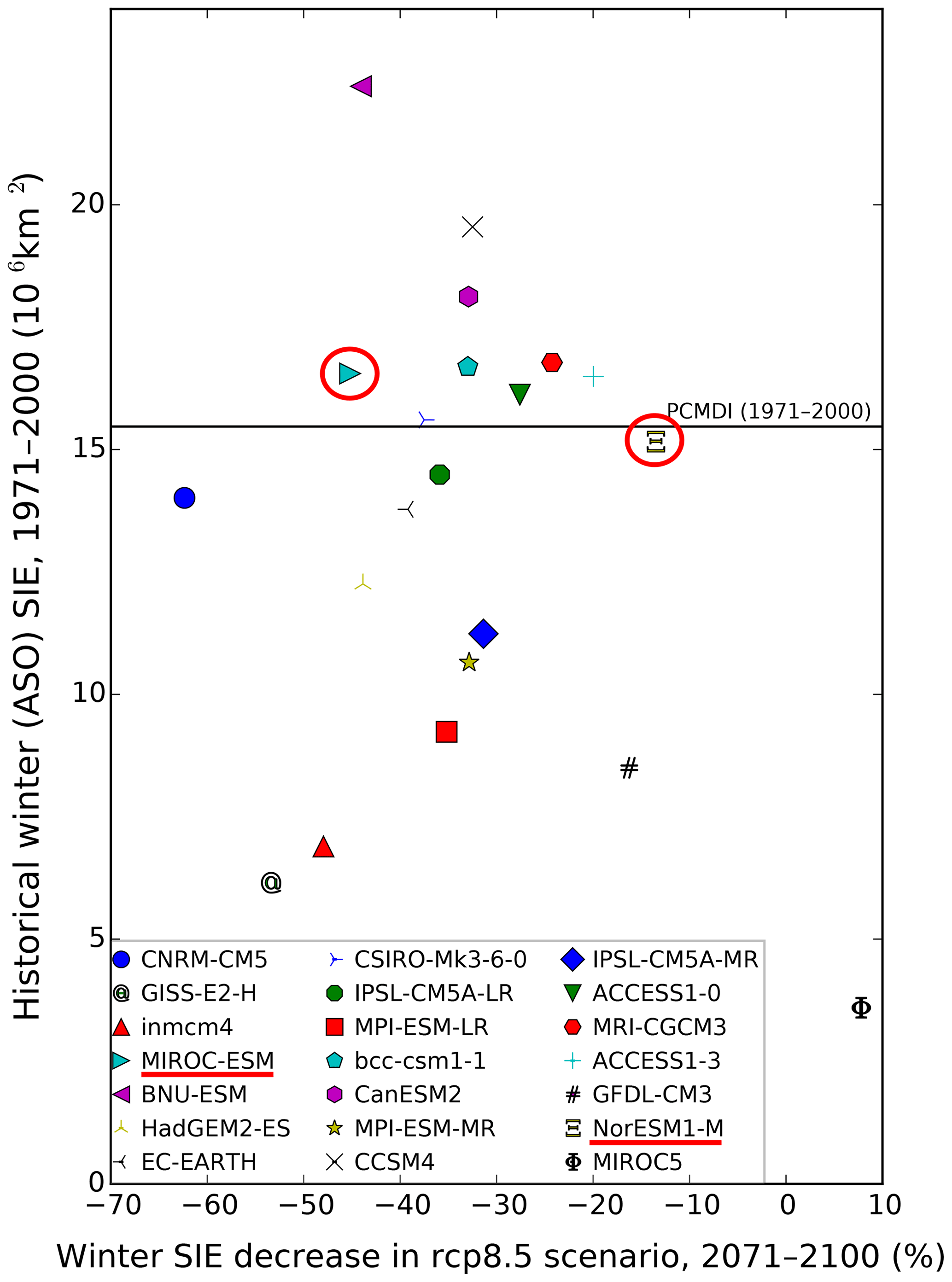
Figure 1 Historical Antarctic winter (August–September–October: ASO) sea ice extent (SIE, in millions of square kilometres) as a function of the relative decrease in winter SIE in the RCP8.5 projection for the period 2071–2100 with respect to the reference period 1971–2000. The mean winter SIE in the observations for the historical reference period is indicated by the horizontal black line (PCMDI 1971–2000). Models selected for this study are highlighted in red.

2.2 CNRM ARPEGE set-up

We use version 6.2.4 of AGCM ARPEGE, a spectral primitive equation model from Météo-France, CNRM (Déqué et al., 1994). The model is run at a T255 truncation with a 2.5 zoom factor and a pole of stretching at 80^∘ S and 90^∘ E. With this setting, the horizontal resolution in Antarctica ranges from 30 km near the stretching pole on the Antarctic Plateau to 45 km at the northern tip of the Antarctic Peninsula. At the Antipodes, near the North Pole, the horizontal resolution decreases to about 200 km. In this model version, the atmosphere is discretised into 91 sigma-pressure vertical levels. The surface scheme is SURFEX ISBA-ES (Noilhan and Mahfouf, 1996), which contains a three-layer snow scheme of intermediate complexity (Boone and Etchevers, 2001) that takes into account the evolution of the surface snow albedo, the heat transfer through the snow layers, and the percolation and refreezing of liquid water in the snowpack. Over the ocean, we use a 1-D version of sea ice model GELATO (Mélia, 2002), which means that no advection of sea ice is possible. The sea ice thickness is prescribed following the empirical parameterisation used in Krinner et al. (1997, 2010) and described in Beaumet et al. (2019a). The use of GELATO is therefore limited to the computation of heat and moisture fluxes in sea-ice-covered regions and also allows us to take into account the accumulation of snow on top of sea ice.

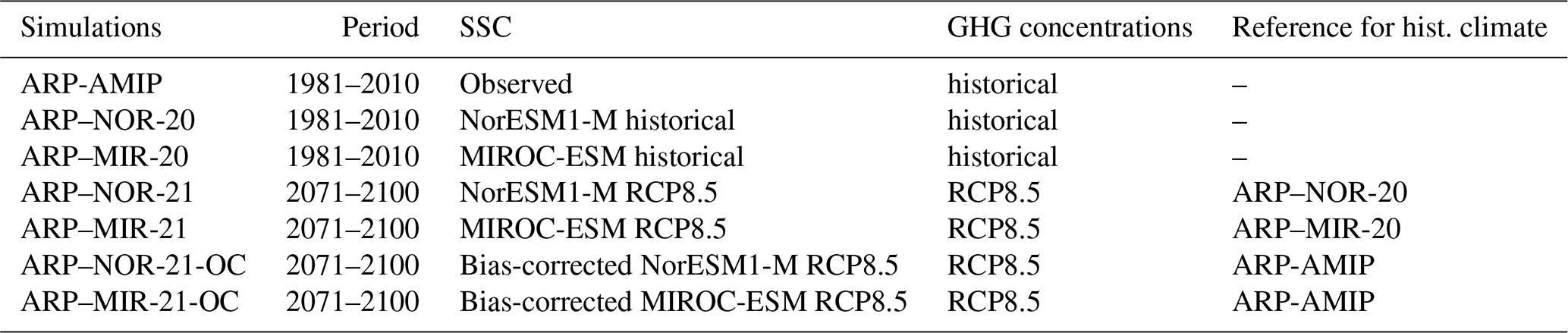
We performed an AMIP-style control simulation for the period 1981–2010 in which CNRM ARPEGE is driven by observed SST and SIC coming from PCMDI data set (Taylor et al., 2000). CNRM ARPEGE was also forced by the original SSCs coming from the historical simulations of MIROC-ESM and NorESM1-M (1981–2010) and from projections under the radiative concentration pathway RCP8.5 (Moss et al., 2010) carried out with the same two models (2071–2100). In each ARPEGE simulation, the first 2 years are considered a spin-up phase for the atmosphere and the soil or snowpack and are therefore discarded from the analysis. The characteristics of the different ARPEGE simulations presented in this paper are summarised in Table 1.

Table 1 Summary of the period, sea surface conditions, greenhouse gas (GHG) concentration and reference historical simulation (for climate projections) for each ARPEGE simulation presented in this paper.

2.3 Model evaluation

The ability of the ARPEGE model to reproduce atmospheric general circulation of the Southern Hemisphere is assessed by comparing sea-level pressure (SLP) and 500 hPa geopotential height (Z500) poleward of 20^∘ S to that of the ERA-Interim reanalysis (ERA-I). For surface climate of the Antarctic continent, several studies have shown that (near-)surface temperatures from ERA-I are not reliable (Bracegirdle and Marshall, 2012; Jones and Harpham, 2013; Fréville et al., 2014), as the reanalysis is not constrained by a sufficient number of observations and because the boundary layer physics of the model fail to successfully reproduce strong temperature inversions near the surface that characterise the climate of the EAP. As a consequence, near-surface temperatures in Antarctica from ARPEGE simulations are evaluated using observations from the SCAR READER database (Turner et al., 2004) as well as temperatures from a MAR RCM simulation in order to increase the spatial coverage of the model evaluation. MAR (Gallée and Schayes, 1994) has been one of the most successful RCMs in reproducing the surface climate of large ice sheets such as Greenland (Fettweis et al., 2005; Lefebre et al., 2005) and Antarctica (Gallée et al., 2015; Amory et al., 2015; Agosta et al., 2018). For Antarctica, outputs of the MAR simulation (version 3.6 of the model) driven by ERA-I have been evaluated against in situ observations for surface pressure, 2 m temperatures, 10 m wind speed, and surface mass balance in Agosta et al. (2018) and Agosta (2018). MAR skills for temperatures and SMB are excellent for most of Antarctica. However, a systematic 3–5 K cold bias over large ice shelves (Ross and Ronne–Filchner) throughout the year and a 2.5 K warm bias over the Antarctic Plateau in winter are worth mentioning.

In this evaluation, we compare ARPEGE near-surface temperatures, to those of an ERA-I-driven MAR simulation (hereafter MAR–ERA-I) at a similar horizontal resolution of 35 km (Agosta et al., 2018). The SMB of the grounded AIS and its components from ARPEGE simulations are compared to the outputs of the same ERA-Interim-driven MAR simulation. We also performed an evaluation of ARPEGE snowfall rates using a model-independent data set such as the CloudSat climatology for Antarctic snowfall (Palerme et al., 2014). However, because this data set is only available for a very short period of time (2007–2010) and is representative of snowfall rates about 1200 m above the surface, the results from this comparison have to be considered with extreme caution and are therefore only shown in the Supplement.

In this study, the statistical significance at the 5 % level of the difference between two samples of independent mean ($\stackrel{\mathrm{‾}}{A}-\stackrel{\mathrm{‾}}{B}$) is admitted when it verifies the following condition:

$$\begin{array}{}\text{(1)}& |\stackrel{\mathrm{‾}}{A}-\stackrel{\mathrm{‾}}{B}|>{\displaystyle \frac{\mathrm{1.96}\times \left(\right({\text{STD}}_A+{\text{STD}}_B)\times \mathrm{0.5})\times \sqrt{\mathrm{2}}}{\sqrt{n-\mathrm{2}}}},\end{array}$$

where STD_A and STD_B are the standard deviation of sample A and B, and n is the size of the sample (usually 30 in this study, because of 30-year simulations).

3 Results

3.1 Simulated present climate

In this section, ARPEGE simulations are evaluated using mostly ERA-I reanalyses for atmospheric general circulation south of 20^∘ S and polar-oriented RCMs as well as READER in situ data for the surface climate of the ice sheet.

3.1.1 Atmospheric general circulation

The differences between mean SLP from the 1981–2010 ARPEGE simulation driven by observed SSCs (called ARP-AMIP in the remainder of this paper; see Table 1) and mean SLP from ERA-I can be seen in Fig. 2a. The general pattern is an underestimation of SLP around 40^∘ S, especially in the Pacific sector (up to 6 to 10 hPa) and an overestimation around Antarctica (generally between 4 and 8 hPa), especially in the Amundsen–Ross sea sector. Mean SLP differences for ARPEGE simulations driven by NorESM1-M (ARP–NOR-20) and MIROC-ESM (ARP–MIR-20) historical SSCs can be seen respectively in Fig. 2b and c. The pattern and the magnitude of the errors are similar to those of the ARP-AMIP simulation in summer (DJF). The seasonal root-mean-square errors (RMSEs) for each simulation are summarised in Table 2. In winter (JJA), spring (SON) and autumn (MAM) the errors are substantially larger in ARP–NOR-20 and ARP–MIR-20 than in ARP-AMIP (up to 50 % larger). The patterns of the errors and the ranking of simulation scores are similar for the 500 hPa geopotential height (not shown).

The mean atmospheric general circulation in each simulation has also been compared and evaluated against ERA-I by analysing the latitudinal profile of the 850 hPa zonal mean eastward wind component (referred to as westerly winds in the following), as well as the strength (m s⁻¹) and position (degrees of southern latitude) of the zonal mean westerly wind maximum (Fig. 3). In this figure, results are only presented for the annual average, as the differences between simulations or with respect to ERA-I do not depend much on the season considered (not shown). ARP-AMIP and ARP–MIR-20 better simulate the westerly wind maximum strength than ARP–NOR-20, with an underestimation of this maximum of about 1.5 m s⁻¹ compared to ERA-I. The equatorward bias on the position of the westerly wind maximum is 1.6^∘ in ARP–NOR-20, while it is up to 3 to 5^∘ in ARP-AMIP and ARP–MIR-20.

Table 2 Seasonal root-mean-square error (RMSE, in hectopascals) on mean SLP south of 20^∘ S with respect to ERA-Interim for the different ARPEGE simulations over the 1981–2010 period. Each error is significant at p=0.05.

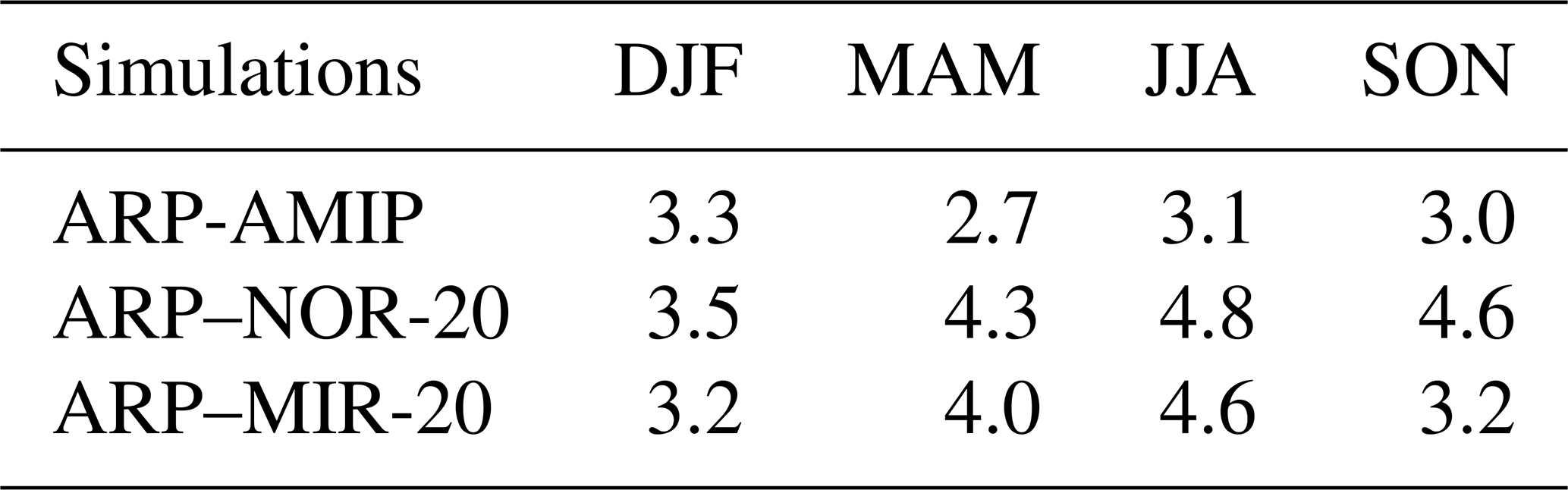
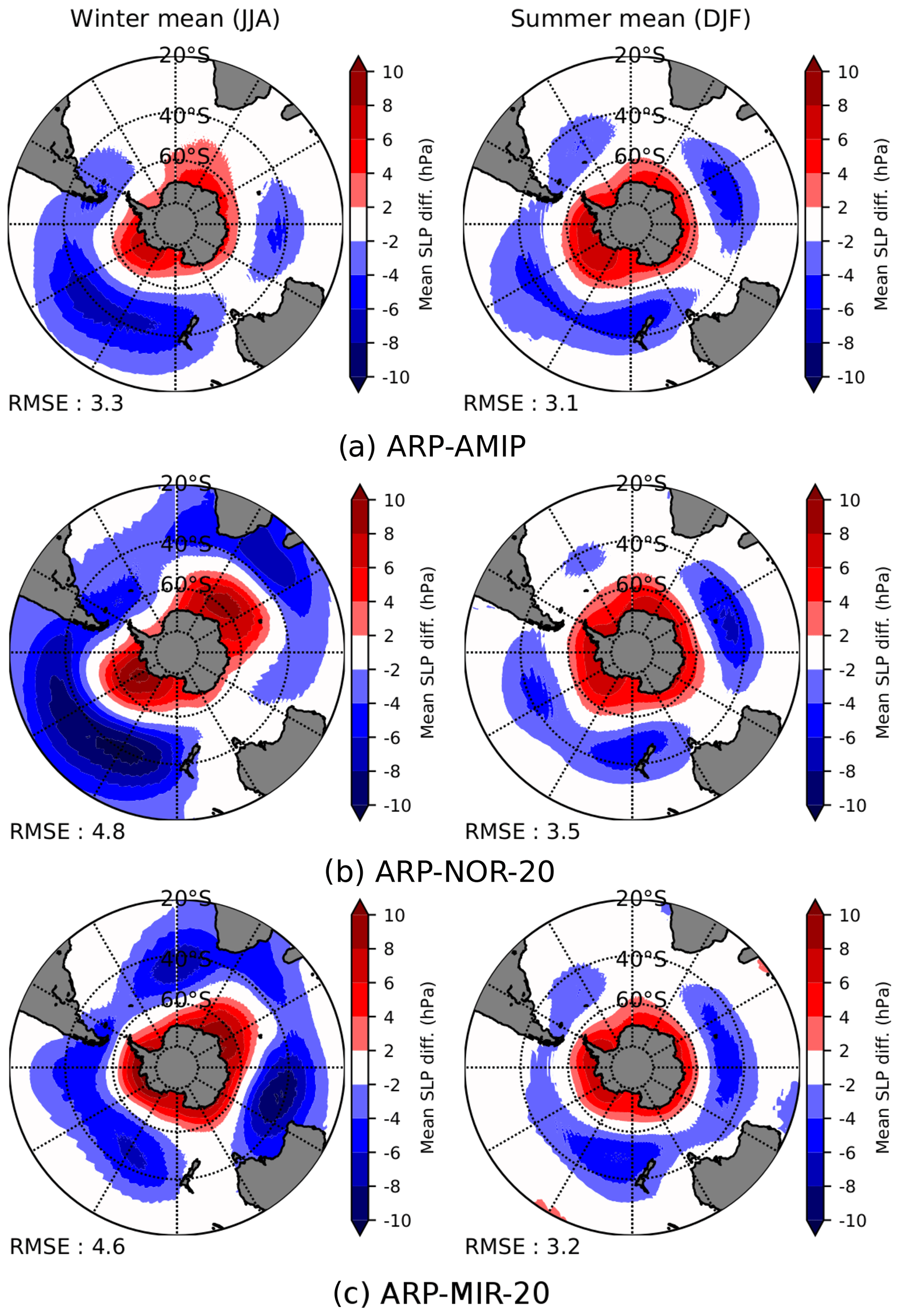
Figure 2 Difference between ARPEGE simulations and ERA-I mean SLP for the reference period 1981–2010 in winter (JJA, left) and summer (DJF, right). Values of the RMSE are given below the plots.

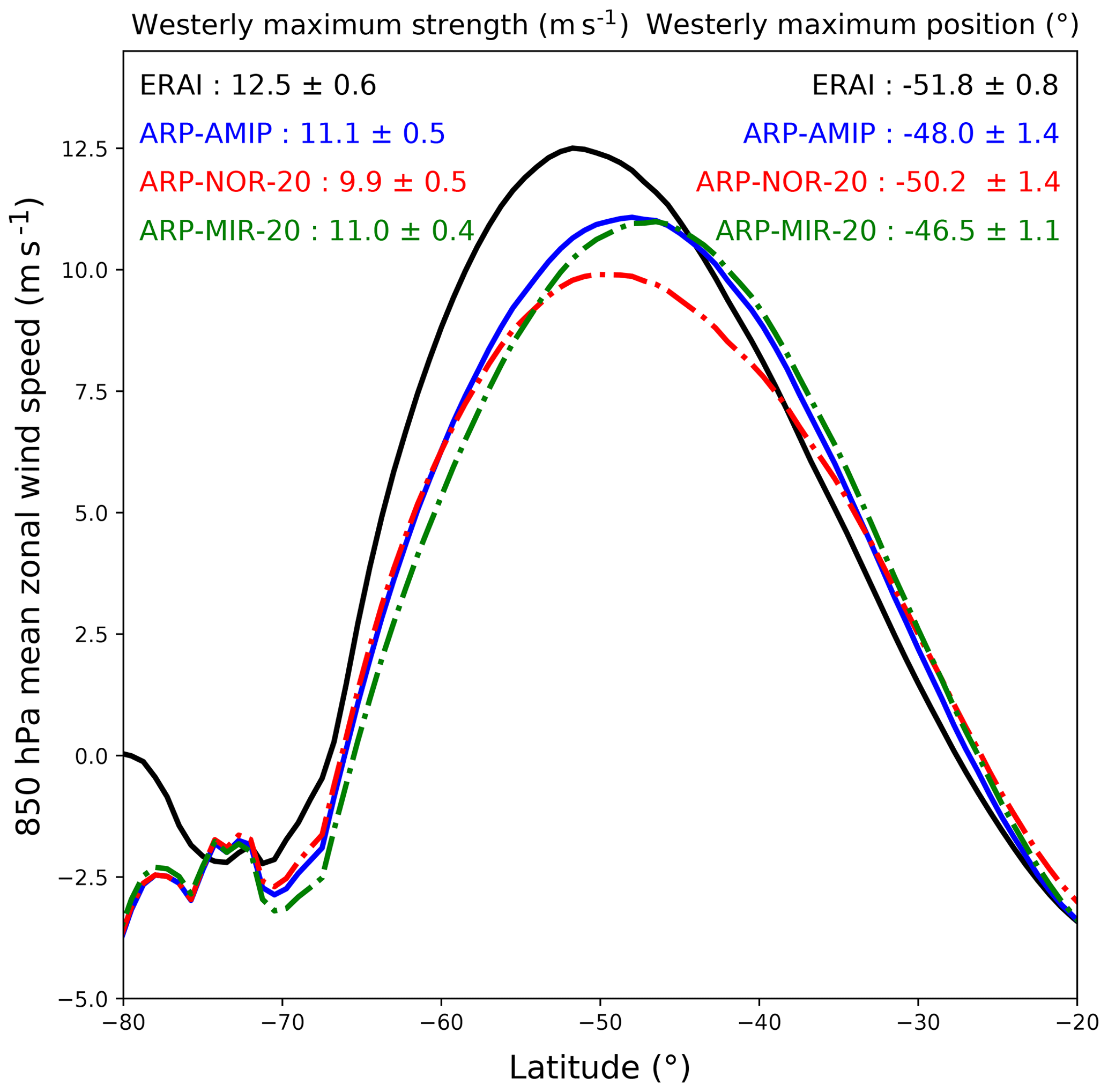
Figure 3 Mean latitudinal profile of 850 hPa eastwards wind component (reference period: 1981–2010) for ARP-AMIP (grey), ARP–MIR-20 (dashed green), ARP–NOR-20 (dashed red) and ERA-Interim (black). Yearly mean ± 1 standard deviation of strength (m s⁻¹, upper left) and latitude position (^∘, upper right) of the 850 hPa westerly wind maximum.

3.1.2 Near-surface temperatures

Screen level (2 m) air temperatures (T_2 m) from the ARP-AMIP simulation are compared to those from the MAR–ERA-I simulation and READER database in winter (JJA) and summer (DJF) for the reference period 1981–2010 (Fig. 4). In this analysis, stations from the READER database for which fewer than 80 % of valid observations were recorded for the reference period were not used. Altitude differences between corresponding ARPEGE grid point and stations have been accounted for by correcting modelled temperatures with a 9.8 K km⁻¹ dry adiabatic lapse rate similarly to in Bracegirdle and Marshall (2012). Errors of the T_2 m in the ARP-AMIP simulation for each weather station and each season are presented in the Supplement.

The ARP-AMIP T_2 m values are much warmer than MAR–ERA-I on the ridge and the western parts of the Antarctic Plateau in winter as well as on the large Ronne and Ross ice shelves. Consistently with its atmospheric circulation errors in this area, ARPEGE is colder than MAR–ERA-I on the southern and western part of the Antarctic Peninsula, especially in winter. We can also mention a moderate (1 to 3 K) but widespread warm bias on the slope of the EAP and on the west side of the West Antarctic Ice Sheet (WAIS) in summer. Except for some coastal stations of East Antarctica, T_2 m errors in the ARP-AMIP simulation are very similar in the comparisons with MAR–ERA-I and the READER database.

Considering errors on near-surface temperatures of the Antarctic Plateau as large as 3 to 6 K for ERA-I reanalysis in all seasons (Fréville et al., 2014), skills of the ARP-AMIP simulation in this region are comparable to those of many AGCMs or even climate reanalyses. The systematic error for the Amundsen–Scott station is for instance not significant at the 5 % level in any season except autumn (MAM). The large discrepancies between ARPEGE and MAR over large ice shelves are further investigated in the Supplement. Although a part (3–5 K) of this large discrepancy in winter (ARPEGE up to 12 K warmer than MAR over the centre of Ross Ice Shelf) comes from a cold bias in MAR identified in the comparison with the in situ observations (Agosta, 2018), the majority of ARPEGE errors on large ice shelves appear to come from specificities in the representation of stable boundary layers over these large and flat surfaces. As a consequence, the surface climate over the large ice shelves simulated by ARPEGE should at this stage be used with circumspection. Considering the lower model skills on the floating ice shelves, integrated SMB and temperature changes are mostly presented and discussed for the grounded AIS in the remainder of the paper.

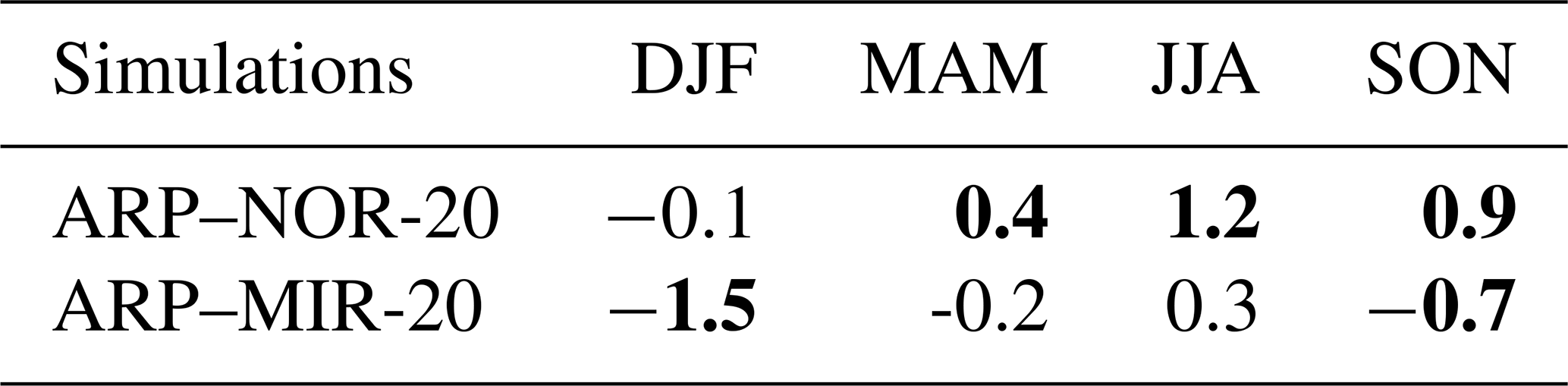
Large negative biases in ARP-AMIP for some coastal stations of East Antarctica (Casey, Davis, Mawson, McMurdo), especially in winter, are likely due to effects of the local topography that cannot be captured at a 35 km horizontal resolution. In addition, ARPEGE temperatures are representative for a 35 km × 35 km inland grid point, whereas many weather stations are located very close to the shoreline. The large cold bias at Rothera station on the peninsula is likely a combination of the effects of poorly represented local topography in the model and of errors on the simulated atmospheric general circulation. Contrary to the continent's interior, the average 35 km horizontal resolution used in this study is insufficient to capture many local topographic features of the coastal areas and of the AP, which challenges the comparisons with in situ measurements in these areas. Regarding T_2 m in ARPEGE simulations forced by NorESM1-M and MIROC-ESM historical SSCs, the skills of the ARPEGE model are particularly impacted over the AP and, to a lesser extent, over the EAP (see Fig. S3 in the Supplement). Over coastal East Antarctic stations, most of the errors in T_2 m are likely due to local topography effects, or inadequacies of the physics of the atmospheric model, as the skills of the atmospheric model show few variations in the three simulations. The use of SSCs from NorESM1-M and MIROC-ESM instead of observed SSCs also impacts the simulated temperatures at the continental scale. Differences for ARP–NOR-20 and ARP–MIR-20 in T_2 m for the grounded AIS with respect to the ARP-AMIP simulation are presented in Table 3. For the ARP–MIR-20, differences of −0.7 K in spring and −1.5 K in summer were found significant. For ARP–NOR-20, differences ranging from 0.4 to 1.2 K in autumn, winter and spring are significant as well.

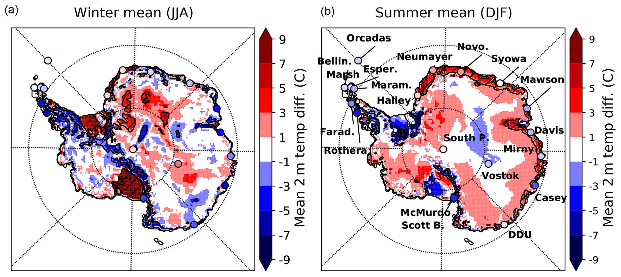
Figure 4 T_2 m differences between ARP-AMIP and MAR–ERA-I (Agosta et al., 2018) simulations in winter (JJA, a) and summer (DJF, b) for the reference period 1981–2010. Circles are T_2 m differences between ARP-AMIP and weather stations from the READER database, station names are shown in (b) (Bellin.: Bellingshausen; DDU: Dumont D'Urville; Esper.: Esperanza; Farad.: Faraday; Maram.: Marambio; Novo.: Novolarevskaya; South P.: South Pole–Amundsen–Scott). Black hatched areas are where $|\text{ARPEGE}-\text{MAR}|=\mathrm{1}\text{MAR}\mathit{\sigma }$.

Table 3 Mean seasonal T_2 m differences (in kelvin) for the grounded AIS with respect to the ARP-AMIP simulation. Differences significant at p=0.05 are presented in bold.

3.1.3 Surface mass balance

In this study, SMB from ARPEGE simulations is defined as the total precipitation minus the surface snow sublimation/evaporation minus the surface run-off. Differences between ARP-AMIP and MAR–ERA-I total precipitation, snow sublimation and SMB (in millimetres of water equivalent per year) for the reference period 1981–2010 can be seen in Fig. 5. As differences in run-off are restricted to the ice shelves and some very localised coastal areas, their spatial distribution is not displayed in this figure. Yearly mean SMB, total precipitation, sublimation, run-off, rainfall and melt, integrated over the whole grounded AIS for the different ARPEGE simulations, for MAR and RACMO2 driven by ERA-Interim reanalyses, and from other studies are presented in Table 4.

Precipitation integrated over the grounded AIS in ARP-AMIP and ARP–MIR-20 is very close to the values from MAR–ERA-I and RACMO2-ERA-I. However, higher surface sublimation (and run-off) in the ARPEGE simulation yields lower estimates of the grounded AIS integrated SMB. Integrated SMB over the ice sheet using ARPEGE, however, concurs with independent estimates from satellite data (e.g. Vaughan et al., 1999; Arthern et al., 2006). Precipitation is generally much higher in ARPEGE with respect to MAR over many coastal areas such as the Ross sector of Marie Byrd Land, in Dronning Maud Land and in the northern and eastern parts of the AP. On the other hand, precipitation is lower in ARP-AMIP in the western part of the peninsula, in the inland part of the central WAIS, and in the interior and lee-side of the Transantarctic Mountains. Sublimation integrated over the grounded AIS is about 3 times higher in ARP-AMIP than in MAR–ERA-I. Differences mostly come from coastal areas and the peripheral ice sheet. This is consistent with ARP-AMIP being systematically 1 to 3 K warmer than MAR–ERA-I in summer in those areas. The inter-annual variability is very high in the simulated ARPEGE run-off, in accordance with MAR–ERA-I. A closer look at the values of rainfall, surface snowmelt and run-off in the three present-day ARPEGE simulations in Table 4 shows that about one-third of the liquid water input into the snowpack (rainfall + surface snowmelt) does not refreeze and therefore leaves the snowpack in the end. In MAR–ERA-I and in RACMO2-ERA-I, this ratio is about 1∕20. This means that although the snow surface scheme SURFEX ISBA-ES used in ARPEGE is in principle able to explicitly account for storage and refreezing of liquid water in the snowpack, the retention capacity of the Antarctic snowpack appears to be largely underestimated when compared to MAR and RACMO2. For these reasons, projected changes in melt rates are preferably presented and discussed in Sect. 3.2, while changes in run-off are not shown due to the suspected lower skill of ARPEGE for this variable and strong non-linearities expected in changes in surface run-offs in a warming climate.

In the ARP–MIR-20 simulation, snow sublimation, run-off and melt were found to be significantly lower than in ARP-AMIP, which is consistent with this simulation being 1.5 K cooler in summer (DJF). The effect of driving ARPEGE with biased SSCs for the modelling of Antarctic precipitation is discussed in the Supplement.

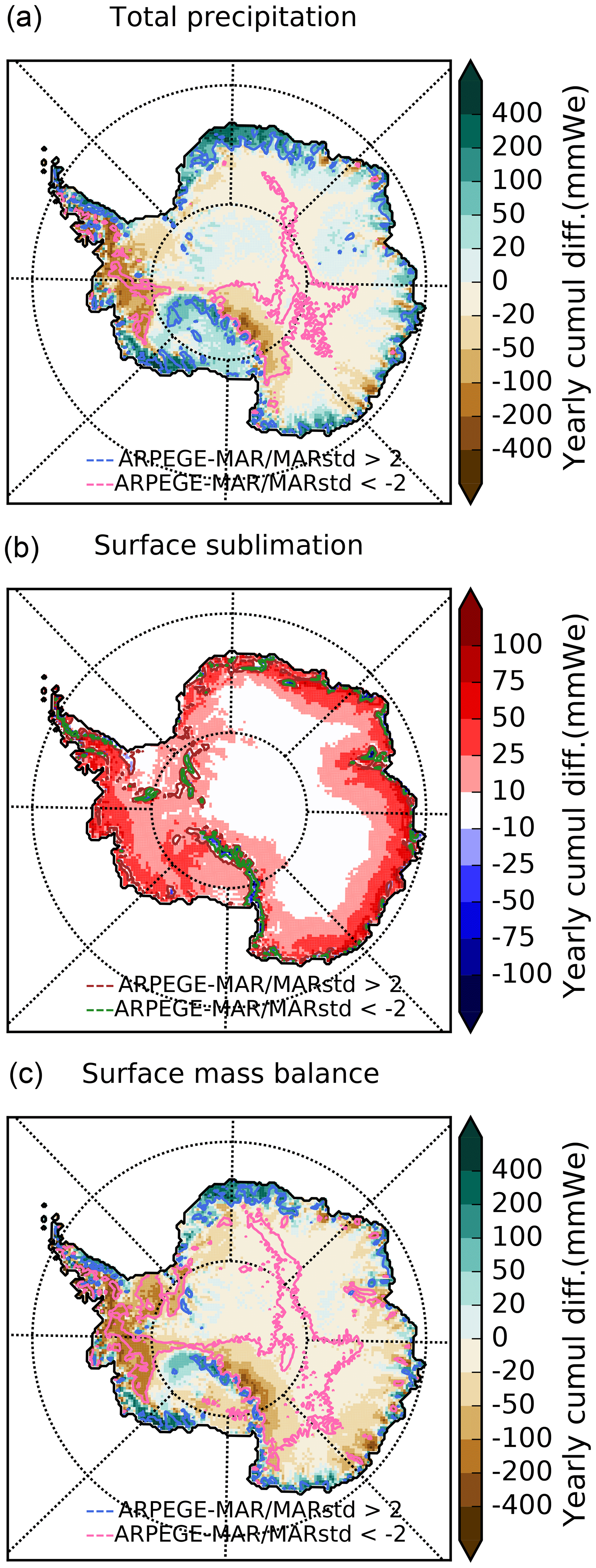
Figure 5 Total precipitation (a), sublimation/evaporation (b) and SMB (c) for the ARP-AMIP minus MAR–ERA-I difference (mm w.e. yr⁻¹) for the reference period 1981–2010. Pink (brown) and blue (green) contour lines represent areas where ARPEGE-MAR absolute differences are respectively larger than 2 MAR standard deviations of the annual mean (2σ).

Vaughan et al. (1999)

Table 4 Mean grounded AIS SMB and its component (Gt yr⁻¹) ± 1 standard deviation of the annual mean for the reference period 1981–2010. Variables from ARP–NOR-20 and ARP–MIR-20 that are significantly different from the value in ARP-AMIP at the p=0.05 level are in bold.

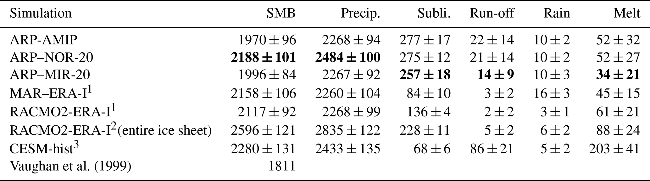
¹ MAR and RACMO2 driven by ERA-I and ARPEGE statistics for 1981–2010 over the grounded AIS are computed using MAR grounded ice mask (area = 12.37 km × 10⁶ km) as in Agosta et al. (2018). Sublimation values for RACMO2 include drifting snow sublimation, while only surface sublimation is accounted for in MAR and ARPEGE statistics. ² RACMO2 statistics are given for the total ice sheet and the period 1979–2005 from Lenaerts et al. (2016); sublimation includes drifting snow sublimation. ³ Community Earth System Model historical simulation (1979–2005) values for the total ice sheet from Lenaerts et al. (2016).

3.2 Climate change signal

In this section, we present the climate change signal obtained in ARPEGE RCP8.5 projections driven by SSCs from NorESM1-M and MIROC-ESM. For ARPEGE projections realised using original SSCs from the two coupled models (ARP–NOR-21 and ARP–MIR-21), the reference simulations for the historical period are the ARPEGE simulations performed with historical SSCs coming from the respective coupled model (ARP–NOR-20 and ARP–MIR-20). For projections realised with bias-corrected SSCs (ARP–NOR-21-OC and ARP–MIR-21-OC), the reference simulation for the historical period is ARP-AMIP (observed SSCs). The primary goal here is to evaluate the effect on the climate change signals for Antarctica simulated by the ARPEGE AGCM associated with SSC forcings coming from two end values of the CMIP5 RCP8.5 ensemble in terms of sea ice retreat, as well as the effect of the bias correction of SSC.

3.2.1 Atmospheric general circulation

Climate change signals in mean SLP for the different RCP8.5 projections realised with ARPEGE can be seen in Fig. 6. All projections show a pressure increase at mid-latitudes (30–50^∘ S) and a decrease around Antarctica. This corresponds to a strengthening of the mid- to high-latitude pressure gradient (positive phase of the SAM) and a poleward shift of the circum-Antarctic low-pressure belt towards the continent, which are generally the expected consequences of 21st century radiative forcing (Kushner et al., 2001; Arblaster and Meehl, 2006). This pattern (increase at mid-latitude, decrease around Antarctica) is sharper in projections realised with MIROC-ESM SSCs.

Differences in the climate change signal between ARP–NOR-21-OC and ARP–NOR-21 are small (Fig. 6a). Differences in SLP changes are larger in the projections realised with MIROC-ESM SSCs: in those with non bias-corrected SSCs (ARP–MIR-21), the intensification of the low-pressure systems around Antarctica in winter is clearly organised in a three-wave pattern (Fig. 6b). In ARP–MIR-21-OC, the JJA pressure decrease is rather organised in a dipole with one maximum of pressure decrease centred on the eastern side of the Ross Sea and the other west of the Weddell Sea. As a result, the three-wave pattern is clearly noticeable in the difference between the two climate change signals (Fig. 6b, right). Late 21st century changes in westerly wind maximum latitude position and strength at 850 hPa are shown in Table 5. When compared to the variability in the reference historical simulations, each climate change signal is significant at the 5 % level. Regarding the changes in westerly wind maximum strength, the differences between the two projections using NorESM1-M SSCs are limited. However, we can mention a 1.4^∘ larger southward displacement of the westerly wind maximum position in the projection using bias-corrected SSCs (significant at the 5 % level). Differences in changes in position and strength are not significant between ARP–MIR-21 and ARP–MIR-21-OC. Compared to projections realised with SSCs from NorESM1-M, these projections show a slightly larger increase in westerlies maximum strength and a much larger poleward shift, although this difference is reduced when comparing projections with bias-corrected SSCs.

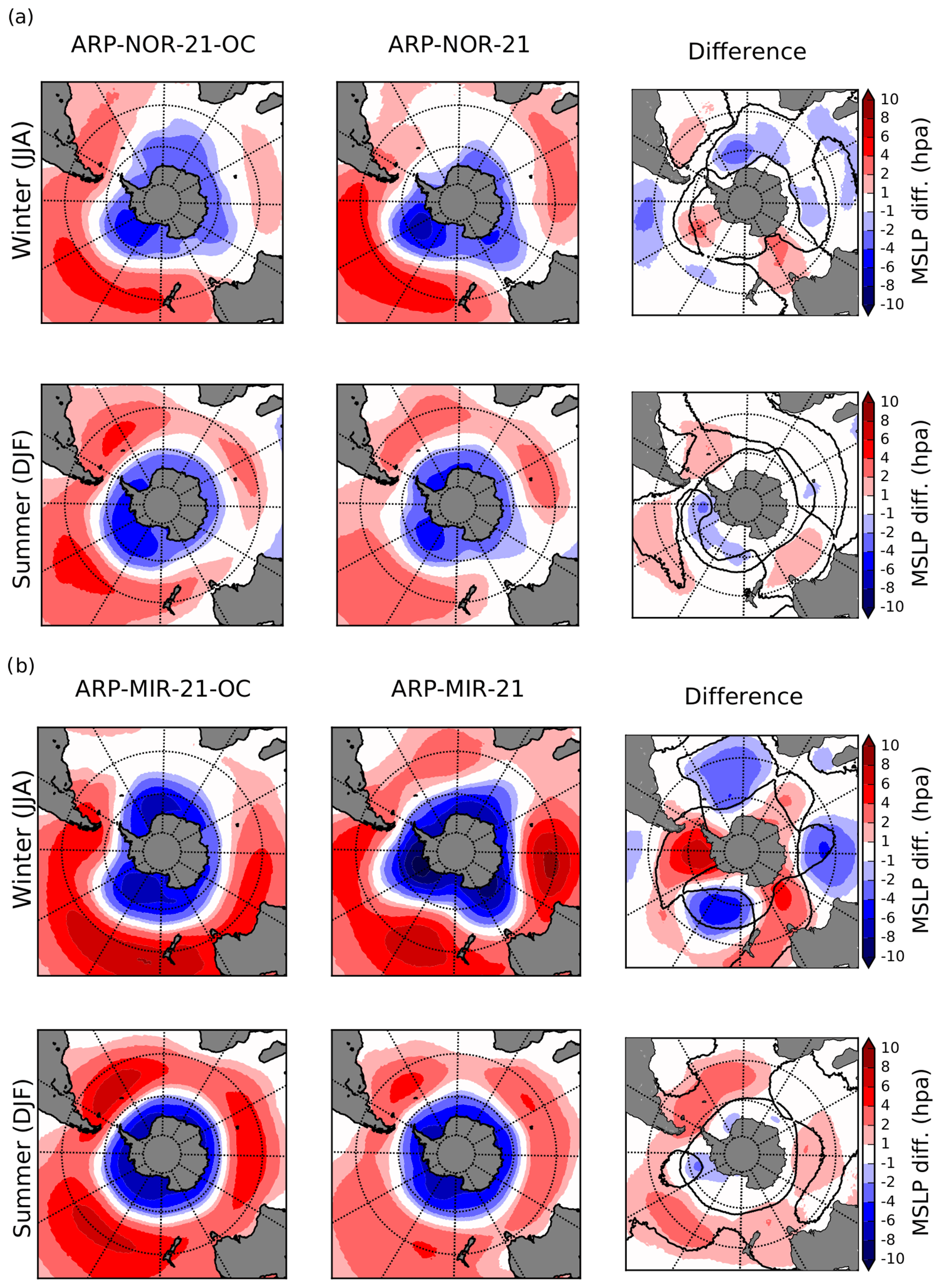
Figure 6 Climate change signal in SLP for ARPEGE RCP8.5 projections with bias-corrected SSCs (left), original SSCs (centre) and difference (right). Climate change signals for winter (JJA) are displayed at the top of the panels and at the bottom for summer (DJF). Results for projections with SSCs from NorESM1-M are presented in the upper part (a) and from MIROC-ESM in the lower part (b) of the figure. Black contour lines represent areas where differences in climate change signal are 50 % of the climate change signal in the simulation with non-bias-corrected SSCs.

Table 5 Changes in mean yearly southern westerly wind maximum strength (ΔJSTR, m s⁻¹) and position (ΔJPOS, ^∘) for the different ARPEGE projections. Changes significantly different using bias-corrected SSCs are shown in bold.

3.2.2 Near-surface temperatures

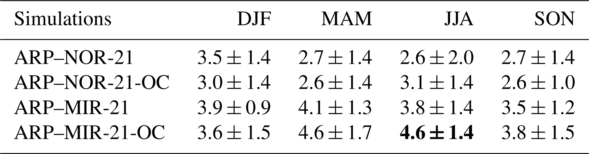
The mean yearly T_2 m increase for the grounded AIS using SSCs from the NorESM1-M RCP8.5 projection is 2.9 ± 1.0 K using original SSCs (ARP–NOR-21) and 2.8 ± 0.8 K using bias-corrected SSCs (ARP–NOR-21-OC). For projections using SSCs from MIROC-ESM, these temperature increases are respectively 3.8 ± 0.7 and 4.2 ± 1.0 K. The differences in yearly T_2 m increase using bias-corrected SSCs are found to be non-significant in both cases. T_2 m increase per season can be seen in Table 6. Only a +0.8 K difference in winter temperature increase in ARP–MIR-21-OC with respect to the projection driven by original SSCs is found significant. At the regional scale (Fig. 7b), this is materialised by large areas of 1 to 2 K stronger warming in the centre of the East Antarctic Plateau, Dronning Maud Land and the Ross Ice Shelf. The difference in warming in ARP–MIR-21-OC is the highest in Marie Byrd Land (+2 K).

For projections using SSCs from NorESM1-M, no seasonal differences were found significant at the AIS scale.

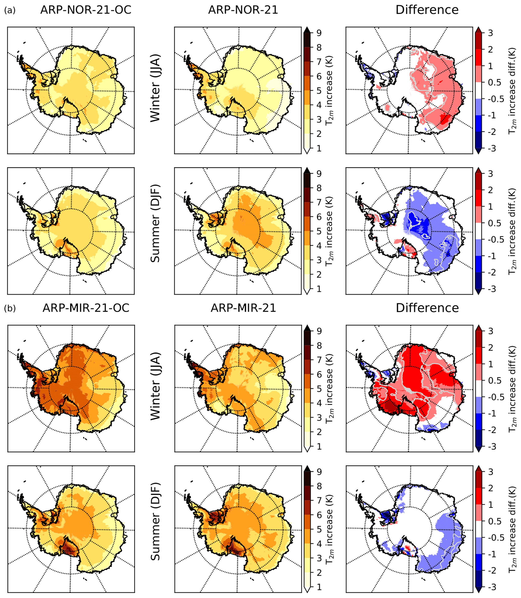
Figure 7 Climate change signal in T_2 m for ARPEGE RCP8.5 projections for the late 21st century (2071–2100) with bias-corrected SSCs (left), original SSCs (centre) and the difference (right). Climate change signals for austral winter (summer) are displayed at the upper (lower) part of the figure. Results for projections with SSCs from NorESM1-M are presented in (a) and from MIROC-ESM in (b). Grey contour lines show where differences in climate change signal are 25 % of the climate change signal using non bias-corrected SSCs.

Table 6 Mean seasonal T_2 m increase (K) for the grounded AIS for the different ARPEGE RCP8.5 projections for the late 21st century (reference period: 2071–2100) with respect to their historical reference simulation (reference period: 2071–2100). Climate change signals in projections with bias-corrected SSCs significantly different at the p=0.05 level are presented in bold.

3.2.3 Precipitation and surface mass balance

Absolute values and changes in grounded AIS SMB and its components for the late 21st century are shown in Table 7. For the experiment realised with NorESM1-M SSCs, precipitation and SMB changes (in both cases increases) are very similar (no significant differences), despite about 220 Gt yr⁻¹ more precipitation and accumulation in ARP–NOR-21 absolute values (significant at p=0.05, Table 7). No significant differences in absolute values or climate change signals were found for the other components of SMB for projections with NorESM1-M SSCs.

For the experiment performed with MIROC-ESM SSCs, absolute values and increase in precipitation are about 170 Gt yr⁻¹ (7 %) stronger in the projection with bias-corrected SSCs. The total precipitation increase is +8.8 % K⁻¹ in ARP–MIR-21-OC, compared to a 7.9 % K⁻¹ increase in ARP–MIR-21. For SMB and precipitation, both absolute values and climate change signals were found significantly different in ARP–MIR-21-OC than in ARP–MIR-21.

In all projections, the sublimation increases by about 20 % to 30 % with respect to the corresponding values in the historical period. Surface melt increases by about a factor of 2 to 3 in projections with NorESM1-M SSCs and by factors from 5 to 6 in projections with MIROC-ESM SSCs. Increases in SMB remain essentially determined by the increases in precipitation. As a consequence, we only present here the spatial distribution of changes in precipitation in Antarctica in Fig. 8. In all projections, the largest absolute precipitation increases occur in the coastal regions of West Antarctica and in the west of the peninsula. In simulations with MIROC-ESM SSCs, precipitation increase is also very large in the Atlantic sector of coastal East Antarctica. The difference between total precipitation increases in ARP–NOR-21 and ARP–NOR-21-OC (Fig. 8a) is small in most regions of Antarctica, except for a stronger increase (or weaker decrease) in Marie Byrd Land, and a weaker increase in Adélie Land in ARP–NOR-21-OC. For the simulations with MIROC-ESM SSCs (Fig. 8b), we can clearly identify an alternation of three regions of higher or lower precipitation increases. This tri-pole pattern can easily be linked to the three-wave pattern in SLP change in ARP–MIR-21, clearly different than the pattern in mean sea-level pressure (MSLP) change in ARP–MIR-21-OC (Fig. 6b). Here again, Marie Byrd Land and Adélie Land are among the areas where large differences are found between simulations with or without bias-corrected SSCs. Winter and spring (and to a lesser extent autumn) are the seasons mostly responsible for differences in precipitation changes between the simulations with MIROC-ESM original SSCs. The relative mean precipitation changes (%) and the associated standard deviation for the four RCP8.5 projections realised in this study can be seen in Fig. 9.

Table 7 Absolute values, absolute change (Abs. change, Gt yr⁻¹) and relative change (Rel. change, %) for mean SMB, precipitation, surface sublimation, rainfall and melt for the grounded AIS for the different ARPEGE RCP8.5 projections (2071–2100). Climate change signals and absolute values significantly different at the p=0.05 level in projections with bias-corrected SSCs are displayed in bold.

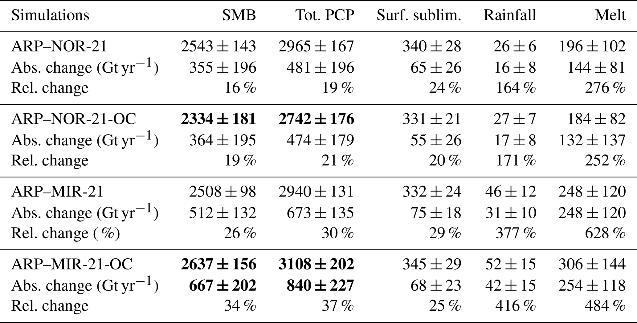
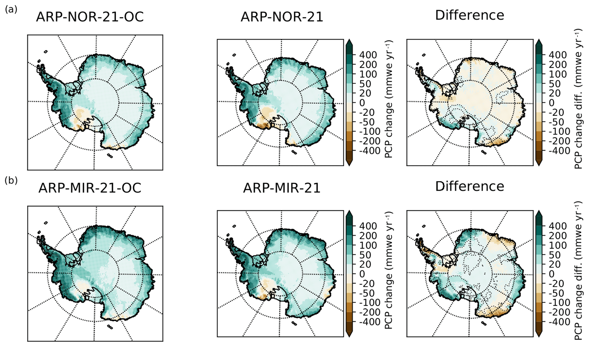
Figure 8 Climate change signal in total precipitation (mm w.e. yr⁻¹) for the late 21st century (reference period: 2071–2100) in the ARPEGE RCP8.5 projection with bias-corrected SSCs (left), original SSCs (centre) and the difference (right). Results for projections with SSCs from NorESM1-M are presented in panel (a) and from MIROC-ESM in panel (b). Dotted lines indicate where the difference is 50 % of the precipitation change in the non bias-corrected SSC projection.

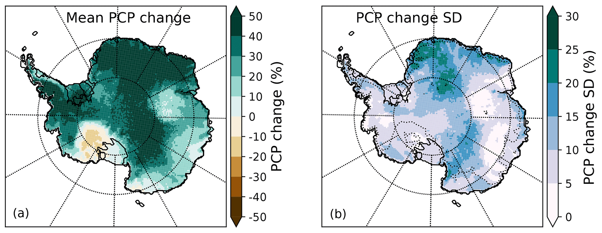
Figure 9 Mean (a) relative precipitation change (%) for the late 21st century from the four ARPEGE RCP8.5 projections and associated standard deviation (b). Dotted lines indicate where the standard deviation is 50 % of the mean change.

4 Discussion

4.1 Evaluation of ARPEGE climate model: reconstruction of historical climate

The atmospheric model ARPEGE correctly captures the main features of the atmospheric circulation around Antarctica. The three local minima in SLP and 500 hPa geopotential height located around 60^∘ W, 90^∘ E and 180^∘ E are well reproduced in the ARP-AMIP simulation (see Fig. S13). However, there is a positive SLP bias in the seas around Antarctica, particularly in the Amundsen Sea low (ASL) sector, and a negative bias at mid-latitudes (30–40^∘ S), especially in the Pacific sector. This bias structure in the Southern Hemisphere is present in many coupled and atmosphere-only GCMs. Its consequence is an equatorward bias on the position of the surface jet associated with westerly winds (Bracegirdle et al., 2013). The errors of our high-resolution ARPEGE on atmospheric general circulation in the high southern latitudes are typical of many lower-resolution climate simulations and of the same order of values as the errors of the CMIP5 and CNRM CM5 and ARPEGE (AMIP) simulations found in Bracegirdle et al. (2013). Even though simulations realised with different versions of the model are to be compared with care, our results suggest that here the use of higher resolution did not improve the representation of the high-southern-latitude atmospheric circulation, contrary to the results of Hourdin et al. (2013), who used the LMDZ model.

The use of observed SSCs (ARP-AMIP) rather than SSCs from NorESM1-M and MIROC-ESM substantially improves the simulated mean SLP in the Southern Hemisphere in all seasons but summer. This confirms at a higher resolution results from previous studies realised at coarser resolution, which have shown that the use of observed rather than modelled SSCs to drive atmosphere-only models clearly improves the skill of the atmospheric models (Krinner et al., 2008; Ashfaq et al., 2011; Hernández-Díaz et al., 2017).

Regarding surface climate, ARPEGE also reasonably reproduces Antarctic T_2 m except over large ice shelves. The T_2 m errors with respect to MAR–ERA-I are generally below 3 K over most of the grounded AIS. There is a substantial warm bias on the top the Antarctic Plateau in winter. However, these errors (+1.5 K at Amundsen–Scott, +3.4 K at Vostok) are to be compared with errors sometimes much larger in other GCMs or even in reanalyses (e.g. Bracegirdle and Marshall, 2012; Fréville et al., 2014). These errors are due to the fact that many climate models fail to capture the strength of the near-surface temperature inversion and the uncoupling with the upper atmosphere when extremely stable boundary layers are formed. The cold bias of ARPEGE in the Antarctic Peninsula, especially in winter, can largely be explained by atmospheric circulation errors, as these lead to an underestimation of mild and moist fluxes from the north-west towards the peninsula.

The grounded AIS total precipitation in the ARP-AMIP simulation is extremely close to the estimates using the MAR or RACMO2 RCMs. However, the higher sublimation (and run-off) rates in the ARPEGE simulation compared to MAR and RACMO2 yield lower SMB values for the grounded AIS. Nevertheless, estimates of the AIS SMB using ARPEGE concur with independent estimates using satellite data (e.g. Vaughan et al., 1999; Arthern et al., 2006). Many of the differences in the spatial distribution of precipitation rates between the ARP-AMIP simulation and MAR–ERA-I are linked to errors in atmospheric general circulations. These are for instance precipitation overestimates by ARPEGE over Marie Byrd Land, the eastern part of the peninsula and Dronning Maud Land, as well as precipitation underestimates over central West Antarctica and the west coast of the peninsula.

4.2 Effects of sea surface conditions

In the historical climate, we found that when driven by SSCs from NorESM1-M instead of observed SSCs, ARPEGE simulates significantly higher precipitation rates at the scale of the ice sheet (+218 Gt yr⁻¹, 2.2σ). When driven by MIROC-ESM SSCs, run-off and snow sublimation were found to be significantly lower than in the other two ARPEGE historical simulations due to cooler temperatures in spring and summer. In the following section, we discuss the effects of SSCs on simulated climate change, the consistency of the atmospheric model response between historical and future climate, and the implication of SSC selection for future Antarctic climate projections.

4.2.1 Climate change signals

NorESM1-M and MIROC-ESM were chosen in this study because they display very different RCP8.5 projections in terms of changes in sea ice around Antarctica (respectively −14 % and −45 % of winter SIE) at the end of the 21st century. The increase in SST below 50^∘ S is much larger in MIROC-ESM (+1.8 K) than in NorESM1-M (+0.4 K). The separate effects of decreases in sea ice cover and increases in SST on Antarctic SMB have been assessed in Kittel et al. (2018) using the MAR RCM. Both result in an increase in Antarctic SMB (precipitation) that mostly takes places over coastal areas, as a result of the increase in evaporation and saturated water vapour pressure and the decrease in the blanket effect of sea ice. van Lipzig et al. (2002) found similar results using the RACMO RCM. In this study, we confirm the high impact of SSCs on Antarctic SMB with a global atmospheric model used at a resolution similar to that commonly used (∼ 30–50 km) for Antarctic studies using RCMs. van Lipzig et al. (2002) have also investigated the separate effects of the surface warming of the ocean and of the homogeneous warming of the atmospheric column at the border of the domain of integration, the latter being more important as a result of increased moisture advection towards the ice sheet over a thicker atmospheric column. These two studies carried out with RCMs driven by climate reanalyses do not account for the response of the atmospheric general circulation to changes in oceanic surface conditions and changes in radiative forcing as expected for the current century. This was carried out in Krinner et al. (2014) using the LMDZ AGCM in a stretched-grid configuration, and it was found that the effects of changes in SSCs on Antarctic precipitation are much larger than the effect of changes in radiative forcings. As in Krinner et al. (2014), we find using an AGCM at a higher resolution that regional precipitation increases depend mostly on the SSC forcing. It was also found in this previous study that the thermodynamic component, which is the changes in precipitation for a given type of atmospheric circulation pattern (due to for instance higher moisture or heat transport as a result of higher SSTs), was more important than the dynamic one, that is the changes in precipitation due to changes in the relative frequencies of atmospheric circulation patterns (see e.g. Driouech et al., 2010) for the projected increase in Antarctic precipitation.

In the projections presented in this study, the Antarctic increase in annual mean T_2 m and the relative increase in precipitation for the late 21st century are within the range of the CMIP5 RCP8.5 projection ensemble (e.g. Palerme et al., 2017). Unsurprisingly, the warming obtained with projections using SSCs from NorESM1-M (around +2.8 K) belongs to the lower end of the values for RCP8.5 CMIP5 projections, a consequence of weaker changes in the Southern Ocean SSCs in this projection. In projections using MIROC-ESM SSCs, the increase in annual T_2 m is around +4 K. The relative increase in precipitation in ARP–MIR-21-OC (+37 %) belongs to the upper limit of the CMIP5 ensemble. As suggested by Krinner et al. (2010), the choice of the AOGCM providing SSCs strongly influences the warming and precipitation increases obtained at the scale of the Antarctic continent. Using NorESM1-M SSCs and uncorrected MIROC-ESM SSCs, the SMB (precipitation) increase obtained with ARPEGE ranges around 5.2 % K⁻¹ (6.6 % K⁻¹ and 7.9 % K⁻¹). This is within the range of values obtained in previous studies (Agosta et al., 2013; Ligtenberg et al., 2013; Krinner et al., 2014; Bracegirdle et al., 2015; Frieler et al., 2015; Palerme et al., 2017). Using bias-corrected SSCs from MIROC-ESM, the sensitivity of the precipitation to temperature increase (8.8 % K⁻¹) is slightly above the higher-end values of previous studies. Yet, this value is consistent with upper values of the CMIP5 ensemble (see  Bracegirdle et al., 2015, Fig. 3), which mostly come from AOGCMs with large SIE in their historical simulations, and consequently a larger decrease in sea ice in their future climate projections (Agosta et al., 2015; Bracegirdle et al., 2015). This suggests that there are some non-linearities in the sensitivity of Antarctic precipitation change to regional warming, as it is also sensitive to the reduced blanket effect of sea ice. Consistent with findings from van Lipzig et al. (2002), we find that for regional warming within the +3 to 4 K range, the increase in SMB is still largely dominated by precipitation increases, which remain much larger than the increase in surface melt and rain.

For the RCP8.5 simulation using SSCs from NorESM1-M, the use of bias-corrected SSCs has not yielded significantly different climate change signals with respect to the simulation using uncorrected SSCs. For future projections with SSCs from MIROC-ESM, using bias-corrected SSCs led to significantly different climate change signals for many variables, especially in winter. In the projection with original MIROC-ESM SSCs, the deepening of the low-pressure zone around Antarctica is mainly organised in a three-wave pattern in JJA, while it shows a dipole in the projection with bias-corrected SSCs. These differences lead to significantly different changes in atmospheric temperatures (0.8 K larger in ARP–MIR-21-OC in winter), the most dramatic difference being the larger (2 K) increase in west Marie Byrd Land using bias-corrected SSCs. Differences in atmospheric circulation are also unsurprisingly associated with significantly different changes in total precipitation. At the continental scale, the increase in moisture advection (approximated trough precipitation minus evaporation, P − E) is 9 % larger in ARP–MIR-21-OC than in ARP–MIR-21. The consequences of the three-wave-pattern decrease in SLP around Antarctica in ARP–MIR-21 are obvious with three regions of lower precipitation increases with respect to ARP–MIR-21-OC. At the regional scale, it is noteworthy that all projections agree on a (slight) precipitation decrease in Marie Byrd Land and the western Ross Ice Shelf (see Fig. 9). The decrease in precipitation in this region is however mitigated when using both sets of bias-corrected SSCs.

A lower increase or a slight precipitation decrease in Marie Byrd Land was also found in other studies (Krinner et al., 2008; Lenaerts et al., 2016). These results, however, bear uncertainties as many free AGCMs (including ARP-EGE) struggle to reproduce the depth and the variability of the ASL. The changes in precipitation (and SMB) in this area are also extremely sensitive to the selected SSCs. The changes in surface climate in the ASL area are extremely important for the SMB of the Antarctic Ice Sheet as a whole as glaciers of the Amundsen Sea Embayment are largely responsible for the positive contribution of the AIS to sea-level rise over recent years (e.g. Shepherd et al., 2018). The melting of ice shelves in this area is also expected to trigger the destabilisation of glaciers located upstream (Rignot et al., 2013; Fürst et al., 2016; Deb et al., 2018).

Climate change signals for temperature and precipitation over large ice shelves (Ross and Ronne–Filchner) do not seem to substantially differ from those in adjacent areas. Yet, as for the reconstruction of recent climate, projected climate change over these areas should be considered with caution, especially for near-surface temperatures.

4.2.2 Consistency of atmospheric model responses

The late winter (August to October, ASO) and late summer (February to April, FMA) errors of historical SST and SIC from NorESM1-M and MIROC-ESM with respect to observations are displayed in the Supplement. The same differences between SSCs of their RCP8.5 projection and their bias-corrected equivalent are also shown. The differences in SSCs used to drive the atmospheric model are, unsurprisingly, extremely similar between historical and future climate experiments. Has the introduction of the same SSC “biases” with respect to the observed or bias-corrected references yielded the same responses of the atmospheric model in the historical and future climates? The consistency of the response of the atmospheric model is considered here as being the key for having the same climate change signals.

For simulations using SSCs from the NorESM1-M model, the consistency of the response of the atmospheric model is clear. The similarities in the differences between ARP–NOR-20 and ARP-AMIP with differences between ARP–NOR-21 and ARP–NOR-21-OC are clear for many climate variables (SLP; see Fig. S14a, c; 500 hPa geopotential, stratospheric temperatures, 500 hPa zonal wind and near-surface atmospheric temperatures). from this perspective, the most interesting feature is that in both historical and future climate, the ARPEGE simulations forced by NorESM1-M original SSCs are about 10 % wetter at the Antarctic continental scale than their bias-corrected reference. The link here between the dynamical response of the atmospheric model and the SST biases of the NorESM1-M AOGCM seems physically consistent. NorESM1-M SSTs are indeed characterised by a warm bias in Southern Hemisphere mid-latitudes (40–60^∘ S) and a cool bias in the southern tropics (see Fig. S2a), which cause a smaller meridional SST gradient. The response of the atmospheric model here is an increase in the moisture transport towards Antarctica (P − E larger by about 10 %) and explains the additional ∼ 200 Gt yr⁻¹ (2σ) of precipitation on the ice sheet in the simulations realised with NorESM1-M uncorrected SSCs. The consistency of the response of the atmospheric model in historical and future climate explains the absence of significant differences in the climate change signals between experiments with the original NorESM1-M SSCs and their bias-corrected reference.

The consistency of the response of the atmospheric model is less clear for the projections realised with SSCs from MIROC-ESM. Some changes in the differences between simulations forced with original SSCs and those forced by their bias-corrected references are noticeable in winter and autumn SLP (Fig. S14b, d) and zonal wind speed (not shown). The main result here, as a consequence of these differences, is a total precipitation difference in the RCP8.5 experiment with bias-corrected SSCs of about +180 Gt yr⁻¹ (∼ 1σ), while there was almost no difference in total precipitation in the historical period between ARP-AMIP and ARP–MIR-20. Here, the link between biases in Southern Hemisphere SST from MIROC-ESM (see Fig. S2b) and the response of ARPEGE appears less clear. SSTs from MIROC-ESM are mainly characterised by a cold bias in the tropics throughout the years. With respect to the ARP-AMIP simulation, ARP–MIR-20 is also characterised by cooler temperatures throughout the tropical troposphere and much lower upper tropospheric and stratospheric temperatures in Antarctica. This suggests that interactions between SST biases, tropical convection and stratospheric meridional temperature gradients could also explain the response of the atmospheric model when forced by MIROC-ESM SSCs-.

4.2.3 Implication of sea surface condition selection

In many cases, it has been reported that selecting the best skilled models for a given aspect of the climate system helps in better constraining the associated uncertainties on the climate change signal (e.g. Massonnet et al., 2012). Here, because we use bias correction of the SSCs, this aspect has reduced importance. While performing a limited number of climate projections, we cover a large range of the uncertainties associated with the evolution of the Southern Ocean surface condition for the Antarctic climate because it was shown to be its primary driver (Krinner et al., 2014). This approach is supported by the fact that biases of large-scale atmospheric circulation of coupled climate models were shown to be highly stationary under strong climate change (Krinner and Flanner, 2018) and that the response of the ARPEGE atmospheric model to the introduction of the same SSC “bias” was shown to be mostly unchanged in future climate. The use of stretched-grid AGCMs and polar-oriented RCMs to downscale future climate projections for Antarctica comports their own assets and drawbacks, and rather than opposed, they could be combined as for Africa in Hernández-Díaz et al. (2017). The warming signal for the AIS in the CMIP5 model ensemble RCP8.5 projection is evaluated to be 4 ± 1 K (Palerme et al., 2017). By selecting NorESM1-M and MIROC-ESM, we explored the range of the Southern Hemisphere SIE changes among the CMIP5 ensemble. However, using these SSCs, the ARPEGE AGCM simulates a warming in the range of 2.8 to 4.2 K, which is in the lower half of the range simulated by the CMIP5 models. Bracegirdle et al. (2015) found that about half of the variance of the CMIP5 projection in the RCP8.5 scenario for Antarctic temperature and precipitation is explained by historical biases and sea ice decreases by the late 21st century. A non-negligible part of the uncertainties of Antarctic climate change is also linked to the representation of general circulation in the atmospheric model (Bracegirdle et al., 2013). This issue should therefore be assessed in future work.

5 Summary and conclusion

This study presented the first general evaluation of the capability of the AGCM ARPEGE to reproduce atmospheric general circulation of the high southern latitudes and the surface climate of the Antarctic Ice Sheet. ARPEGE is able to correctly represent the main features of atmospheric general circulation, although we have shown a negative bias in sea-level pressures at mid-latitudes and a positive bias around Antarctica, especially in the Amundsen Sea sector. Unsurprisingly, the use of observed sea surface conditions (ARP-AMIP simulation) rather than SSCs from NorESM1-M and MIROC-ESM helped to improve the representation of sea-level pressures in the southern latitudes in all seasons but summer. ARPEGE is also able to correctly reproduce surface climate of Antarctica except for large ice shelves. The differences in T_2 m with polar-oriented RCM MAR and in situ observations are encouraging, especially given the large biases that are exhibited in other GCMs or even reanalyses when Antarctic surface climate is considered (Fréville et al., 2014; Bracegirdle and Marshall, 2012). Regarding precipitation, our estimates at the continental scale agree with estimates from other studies such as those using MAR or RACMO2, even though higher sublimation and run-off rates in ARPEGE yield smaller estimates of the grounded AIS SMB by about 150 Gt yr⁻¹ (1.5σ). Concerning regional patterns, the distribution of precipitation in the ARP-AMIP simulation differs from the one in the MAR RCM mainly as a consequence of errors in atmospheric general circulation.

The future climate projections presented in this study are among the first Antarctic climate projections realised at a “high” (Cordex-like) horizontal resolution using a global atmospheric climate model. Concerning climate change signals, we evaluate the impact of using original and bias-corrected sea surface conditions from MIROC-ESM and NorESM1-M, which display opposite trends in their RCP8.5 projections for the Southern Ocean's late 21st century SIE (respect. −45 % and −14 % for winter SIE). Using SSCs from the NorESM1-M model, no significant differences in yearly or seasonal mean T_2 m increase, precipitation or SMB changes were found when using bias-corrected SSCs. When using SSCs directly from the MIROC-ESM model, the increase in precipitation is +30 %, and it reaches +37 % when using the corresponding bias-corrected SSCs. This difference is statistically significant and is linked with clearly different dynamical and thermodynamical changes in SLP around Antarctica, occurring mainly in winter and spring. At the regional scale, large differences in T_2 m and precipitation increases are found when using bias-corrected SSCs from both NorESM1-M and MIROC-ESM.

The analysis of the climate projections further evidences the potential of the ARPEGE model for the study of Antarctic climate and climate change. When using SSCs from NorESM1-M, we found 10 % higher precipitation rates at the continent scale (which is detrimental to the model skills for precipitation) with respect to the bias-corrected reference in both historical and future climate. These findings advocate once more for the use of bias-corrected SSCs to drive climate projections using an AGCM. Additionally, this method reduces the uncertainty of the baseline (historical) climate and the need for computational resources as only one historical simulation using observed SSCs is needed.

In this study, we confirm the importance of the coupled model choice from which SSC projections are taken. By performing bias correction of SSCs, we showed that not only the regional pattern of temperature and precipitation changes can be different but also the integrated changes in SMB and seasonal temperatures at the ice sheet scale. Unsurprisingly, projections using climate change signal from MIROC-ESM SSC projections (larger decrease in sea ice) show higher increases in temperature and precipitation than those using NorESM1-M SSCs. This confirms the effect of sea ice decreases and SST increases on Antarctic temperatures and SMB in a “realistic” climate projection experiment. For the range of Antarctic warming obtained (+3 to +4 K), we confirm results from previous studies showing that the increase in SMB is largely dominated by increases in snowfall, which remain much larger than the increase in melt and rainfall at the ice sheet scale. Considering changes in SIE at the two extreme end values from the CMIP5 ensemble, differences in Antarctic warming obtained (∼ 1 K) are clearly smaller than the spread of CMIP5 projections for the AIS. This is consistent with the fact that a large part of the CMIP5 diversity for Antarctic climate projections comes from atmospheric model (errors) and associated uncertainties. Climate projections presented in this study still bear considerable uncertainties. These mostly come from ARPEGE errors (even when driven by observed SSCs) on southern-high-latitude general atmospheric circulation, which casts some doubt on the reliability of the projected Southern Hemisphere atmospheric circulation changes. As a consequence, in future work, we will assess the impact of AGCM atmospheric circulation errors by performing an ARPEGE simulation nudged towards the reanalysis and use the statistics of the model drift in this nudged simulation as performed in Guldberg et al. (2005) to perform an atmosphere bias-corrected ARPEGE historical simulation. Bias-corrected projections such as in Krinner et al. (2019) can then also be assessed using the method presented in this study.