the Creative Commons Attribution 4.0 License.
the Creative Commons Attribution 4.0 License.
 | 19 Jul 2019
Induced surface fluxes: a new framework for attributing Arctic sea ice volume balance biases to specific model errors
Mat Collins
Ed Blockley
Jeff Ridley
Alejandro Bodas-Salcedo
A new framework is presented for analysing the proximate causes of model Arctic sea ice biases, demonstrated with the CMIP5 model HadGEM2-ES (Hadley Centre Global Environment Model version 2 – Earth System). In this framework the Arctic sea ice volume is treated as a consequence of the integrated surface energy balance, via the volume balance. A simple model allows the local dependence of the surface flux on specific model variables to be described as a function of time and space. When these are combined with reference datasets, it is possible to estimate the surface flux bias induced by the model bias in each variable. The method allows the role of the surface albedo and ice thickness–growth feedbacks in sea ice volume balance biases to be quantified along with the roles of model bias in variables not directly related to the sea ice volume. It shows biases in the HadGEM2-ES sea ice volume simulation to be due to a bias in spring surface melt onset date, partly countered by a bias in winter downwelling longwave radiation. The framework is applicable in principle to any model and has the potential to greatly improve understanding of the reasons for ensemble spread in the modelled sea ice state. A secondary finding is that observational uncertainty is the largest cause of uncertainty in the induced surface flux bias calculation.
- Article
(8761 KB) - Full-text XML
-
Supplement
(273 KB) - BibTeX
- EndNote


The works published in this journal are distributed under the Creative Commons Attribution 4.0 License. This license does not affect the Crown copyright work, which is re-usable under the Open Government Licence (OGL). The Creative Commons Attribution 4.0 License and the OGL are interoperable and do not conflict with, reduce or limit each other.
© Crown copyright 2019
The Arctic sea ice cover has witnessed rapid change during the past 30 years, with a decline in the September extent of 1.05×10⁶ km2 per decade from 1986 to 2015 (HadISST1.2, Rayner et al., 2003). In association with the changes in extent, Arctic sea ice thinning has been observed from submarine and satellite data (Rothrock et al., 2008; Lindsay and Schweiger, 2015). Arctic sea ice has also become younger on average as older ice has been lost (Maslanik et al., 2011), the onset of summer melt has become earlier in the year (Markus et al., 2009) and the onset of winter freezing has become later (Stammerjohn et al., 2012).
The changes have focussed interest on model projections of Arctic sea ice, the loss of which influences the climate directly through increased absorption of shortwave (SW) radiation during summer and through greater release of heat from the ocean to the atmosphere during winter (Stroeve et al., 2012b). However, substantial spread remains in model simulations of present-day Arctic sea ice and of the long-term rate of decline under climate change (Stroeve et al., 2012a). The causes of this spread are poorly understood, resulting in large uncertainty in future projections of Arctic sea ice.
Evaluating sea ice extent or volume with respect to reference datasets shows that some models reproduce present-day sea ice state more accurately than others (e.g. Wang and Overland, 2012; Massonnet et al., 2012; Shu et al., 2015). However, an accurate simulation of sea ice extent and volume under the present-day climate does not necessarily imply an accurate future projection of sea ice change, as a correct simulation can occur through cancelling model errors. Sea ice extent in particular is known to be a very unsuitable metric for diagnosing model performance due to its high internal variability (Notz, 2015; Swart et al., 2015). Hence there is a need to better understand the drivers which lead a model to simulate a given Arctic sea ice state.
This study presents a new framework (the induced surface flux, ISF, framework) to improve understanding of sea ice model bias by identifying proximate drivers of model bias in sea ice volume balance. (Throughout this study we use the term volume balance to describe changes in sea ice volume rather than the more commonly used term mass balance.) The framework is motivated in the following way. Sea ice volume balance is determined by the surface and basal energy balance; assuming constant ice density, the ice volume is to first-order approximation proportional to the energy required to melt the ice. Basal melting of the interior ice pack results primarily from direct solar heating of the ocean (e.g. Maykut and McPhee, 1995), and basal freezing results primarily from conduction of energy upward through the ice (Perovich and Elder, 2002). The total downwards surface energy flux (surface flux) thus contains the principal sources and sinks of energy for the sea ice volume balance on an Arctic-wide scale.
However, interactions between sea ice thickness and surface energy balance, via the surface temperature and surface albedo, give rise to the thickness–growth feedback (Bitz and Roe, 2004) and the surface–albedo feedback (Bitz, 2008), both of which exert first-order control on the sea ice state. Hence, components of the surface energy balance (SEB) cannot be viewed as independent of the sea ice state but are directly affected by it. To resolve this, we need to separate surface flux biases that arise from the sea ice state (representing feedbacks of the sea ice volume balance) from those that represent forcings on the sea ice volume balance.
In the proposed ISF framework, the total downwards surface energy flux is expressed as an explicit function of key Arctic climate model metrics, allowing the dependence of modelled surface flux on each metric to be described. Reference datasets (observational estimates or model reanalyses) then allow the model bias in surface flux induced by the model bias in each model metric to be estimated. Attribution of biases in ice growth and melt over the course of the year is then possible for specific model quantities. The method allows the contributions to model biases in ice growth and melt caused by the surface–albedo feedback, the ice thickness–growth feedback and “forcings” to be independently quantified. In this way it can be seen how model biases in the external forcings drive model bias in the sea ice volume balance, offering a valuable tool for setting sea ice state biases in context and for understanding spread in sea ice simulation within multi-model ensembles.
The ISF framework works by expressing the total downward surface energy flux Fsfc, at each point in time t and space x, as an explicit function gx,t of quasi-independent climate variables vi. The variables are quasi-independent in the sense that while they affect each other on timescales varying from days to months, they affect the surface flux instantaneously. Taking partial derivatives, the dependence of the surface flux on each variable can be separately expressed as (. Given an estimate of the model bias in any variable via a reference dataset , this can be multiplied by the field of surface flux dependence to produce an estimate of the surface flux bias induced (instantaneously) by the model bias in that variable, as a function of space and time.
This method has two key strengths. Firstly, the fields of induced surface flux bias (ISF bias) can be averaged in time or space to determine the large-scale effects of particular model biases. This bypasses nonlinearities in the dependence of surface flux on some model metrics. Secondly, the effects of each on the surface flux are separated such that the sum of the ISF biases theoretically approaches the total (true) model surface flux bias. This is logically implied by the dependent variables affecting the surface flux instantaneously but only affecting each other over longer timescales.
The analysis is applied to the four members of the historical ensemble of the coupled CMIP5 model HadGEM2-ES (Hadley Centre Global Environment Model version 2 – Earth System). As demonstrated below, this model simulates anomalously low annual minimum ice extent, and ice volume that is both too low in the annual mean and too amplified in the seasonal cycle, which is a similar behaviour to that identified by Shu et al. (2015) in the CMIP5 ensemble mean. A variety of reference datasets demonstrate the large observational uncertainties present in the Arctic, which affect our ability to attribute sea ice volume balance bias with the ISF framework.
The paper is structured as follows. In Sect. 2, the HadGEM2-ES model and the reference datasets used are described in turn. In Sect. 3, the sea ice and surface radiation simulations of HadGEM2-ES are evaluated. The demonstration of the sea ice volume balance biases of HadGEM2-ES, as well as possible drivers, motivates the following analysis. In Sect. 4, the ISF framework is described in more detail and examples are shown. In Sect. 5 the ISF analysis is applied to HadGEM2-ES, allowing the role of each model bias identified in Sect. 3 and causing sea ice volume balance bias to be quantified. In Sect. 6 the implications of the results are discussed, in particular the mechanisms by which the identified external drivers determine the modelled sea ice state and the likely drivers behind the corresponding model biases. Conclusions are presented in Sect. 7.
2.1 The HadGEM2-ES model
HadGEM2-ES is a coupled climate model employing additional components to simulate terrestrial and oceanic ecosystems, and tropospheric chemistry (Collins et al., 2011). It is part of the HadGEM2 “family”, a collection of models that all use the HadGEM2-AO coupled atmosphere–ocean system. HadGEM2-AO is developed from HadGEM1 (Johns et al., 2006), a coupled atmosphere–ocean model whose sea ice extent verified well against observations (Wang and Overland, 2009). While the atmospheric and ocean components of HadGEM2-ES contain a large number of improvements relative to HadGEM1, many of these targeted at improving simulations of tropical weather, the sea ice component is very similar to that of HadGEM1 (except for three minor differences, summarized in Martin et al., 2011, Table A4).
A fundamental feature of the sea ice component of HadGEM2-ES is the sub-grid-scale sea ice thickness distribution (Thorndike et al., 1975). In this formulation, ice in each grid cell is separated into five thickness categories with boundaries at 0, 0.6, 1.4, 2.4, 3.6 and 20 m, each with its own area, thermodynamics and surface exchange calculations. Another key aspect of the sea ice model is the zero-layer thermodynamics scheme (appendix to Semtner, 1976), in which the sea ice surface temperature responds instantaneously to changes in forcing, with conduction being uniform within the ice and snow column, and neither sea ice nor overlying snow has heat capacity (sensible heat storage is parameterized in the top 10 cm of the snow–ice column during surface exchange calculations to aid stability).The HadGEM2-ES sea ice model also includes elastic–viscous–plastic sea ice dynamics (Hunke and Dukowicz, 1997) and incremental remapping (Lipscomb and Hunke, 2004). Most sea ice processes are calculated in the ocean model, but the surface energy balance (SEB) calculations are carried out in the atmosphere model, which passes top melting flux and conductive heat flux to the ocean model as forcing for the remaining components. A more complete description of the sea ice component can be found in McLaren et al. (2006).
This study uses the four ensemble members of the CMIP5 historical simulation of HadGEM2-ES, forced with observed solar, volcanic and anthropogenic forcing from 1860 to 2005. The period of 1980–1999 is used for the model evaluation, and all analyses are carried out with data restricted to the Arctic Ocean region. The Arctic Ocean is defined as the area enclosed by the Fram Strait, the northern boundary of the Barents Sea, the eastern boundary of the Kara Sea, the Bering Strait and the northern edge of the Canadian Arctic Archipelago (Fig. 1).

Figure 1The Arctic Ocean region used in the analysis, defined as the area enclosed by the Fram Strait, Bering Strait and the northern boundary of the Barents Sea.
2.2 Reference datasets
Observational uncertainty in the Arctic is greater than in the temperate and tropical regions. There are severe practical difficulties with collecting in situ data on a large scale over regions of ice-covered ocean. While satellites have in many cases been able to produce Arctic-wide measurements, most notably of sea ice concentration, the relative lack of in situ observations against which these can be calibrated means knowledge of the observational errors is limited. Reanalysis data over the Arctic are also more subject to model errors than in other regions, due to errors in atmospheric forcing, and the existence of fewer direct observations available for assimilation (Lindsay et al., 2014). The approach of this study is to use a wide range of observational data to evaluate modelled sea ice state and surface radiative fluxes, constrained where possible, by in situ validation studies. The same datasets are used as reference datasets for the induced surface flux framework.
To evaluate modelled sea ice concentration, we use the HadISST1.2 dataset (Rayner et al., 2003), derived from passive microwave observations. To evaluate modelled sea ice thickness Arctic-wide, we use the Pan-Arctic Ice Ocean Modeling and Assimilation System (PIOMAS) (Zhang and Rothrock, 2003), which is forced with the National Centers for Atmospheric Prediction (NCEP) reanalysis and assimilates ice concentration data. Laxon et al. (2013) and Wang et al. (2016) found PIOMAS to estimate anomalously low winter ice thicknesses compared to satellite observations over some years. In particular, Wang et al. (2016) found PIOMAS to have a mean bias of −0.31 m relative to observations from the ICESat (Ice, Cloud and land Elevation Satellite) laser sensor. To set the PIOMAS comparison in context, we use two additional datasets to evaluate the model over smaller regions: measurements from radar altimetry aboard the European remote sensing (ERS) satellites from 1993 to 2000 (Laxon et al., 2003), limited to latitudes below 82∘ N, and estimates compiled by Rothrock et al. (2008), derived from a multiple regression of submarine transects over the central Arctic Ocean from 1975 to 2000.
To evaluate modelled surface radiative fluxes across the whole Arctic Ocean, three datasets are used. Firstly, we use the CERES–EBAF (Clouds and Earth's Radiant Energy Systems – Energy Balanced And Filled) dataset (Loeb et al., 2009), based on direct measurements of top-of-atmosphere radiances from EOS sensors aboard NASA satellites, available from 2000 to present. Secondly, we use the ISCCP-FD (International Satellite Cloud Climatology Project FD-series) product (Zhang et al., 2004). Lastly, we use the ERA-Interim (ERAI) atmospheric reanalysis dataset, which provides gridded surface flux data from 1979 to present using a reanalysis system driven by the ECMWF (European Centre for Medium-Range Weather Forecasts) IFS forecast model and the 4D-Var data assimilation system (Dee et al., 2011).
In situ validation of these datasets in the Arctic has been limited, but Christensen et al. (2016) found CERES to perform quite well relative to other products, albeit underestimating downwelling longwave (LW) fluxes from November to February by 10–20 Wm−2 relative to in situ observations at Point Barrow (Alaska). Liu et al. (2005) found ISCCP-FD to simulate SW radiative fluxes fairly accurately relative to observations from SHEBA (Surface Heat and Energy Budget of the Arctic) but found it to underestimate] downwelling SW fluxes in spring by over 30 Wm−2, also to overestimate downwelling LW fluxes in winter by around 40 Wm−2. Lindsay et al. (2014) identified ERAI as producing a relatively accurate simulation of surface fluxes compared to in situ observations at Point Barrow (Alaska) and Ny-Ålesund (Svalbard), although it tends to underestimate downwelling SW fluxes in the spring by up to 20 Wm−2 and overestimate downwelling LW fluxes in the winter by around 15 Wm−2. Comparison of winter downwelling LW fluxes in all datasets to in situ measurements compiled by Lindsay (1998) suggests that while ISCCP-FD is likely to be biased high, ERAI and CERES may be relatively accurate.
In addition to the datasets above, in Sect. 4 we make use of satellite estimates of date of melt onset over sea ice (Anderson et al., 2011), also derived from passive microwave sensors. In Sect. 5, to evaluate the impact of observational uncertainty in the ice area, we use the NSIDC “Sea Ice Concentrations from Nimbus-7 SMMR and DMSP SSM/I-SSMIS Passive Microwave Data, Version 1” (Cavalieri et al., 1996) and HadISST.2 (Hadley Centre Ice and Sea Surface Temperature dataset) (Titchner and Rayner, 2014). Finally, in Sect. 6, the CERES-SYN (Synoptic Radiative Fluxes and Clouds) dataset (Rutan et al., 2015), similar to CERES-EBAF but available at higher temporal resolution, is used to examine modelled surface radiation evolution during May in more detail.
In this section, and throughout the rest of the paper, a difference between a model simulation of a particular quantity, and any reference dataset for that quantity, is referred to as a “bias”. In a similar way, the difference in model surface flux judged to arise from the difference in a particular quantity relative to a reference dataset is referred to as an “induced surface flux bias”. Attention is drawn to the fact that, due to observational inaccuracy, true model bias relative to the real world may be somewhat different from the biases described in this way.
Modelled September sea ice extent in HadGEM2-ES from 1980 to 1999 is systematically lower than that observed (Fig. 2a); the four members of the HadGEM2-ES historically forced ensemble simulate a mean September sea ice extent of 5.78×10⁶ km2, with ensemble standard deviation of 0.24×10⁶ km2. By comparison, the mean observed September sea ice extent over this period was 6.88×10⁶ km2 according to the HadISST1.2 dataset.

Figure 2(a) HadGEM2-ES 1980–1999 mean Arctic Ocean ice extent, compared to HadISST1.2 1980–1999, with September ice fraction bias map. (b)–(d) HadGEM2-ES ice thickness compared to (b) PIOMAS 1980–1999, (c) Envisat 1993–1999 and (d) submarine datasets from 1980 to 1999 over respective regions and periods of coverage, with April and October ice thickness bias maps. For each seasonal-cycle plot, the model is in black and reference datasets in red. In (c), data are not plotted from May to September due to the region of coverage being very small.
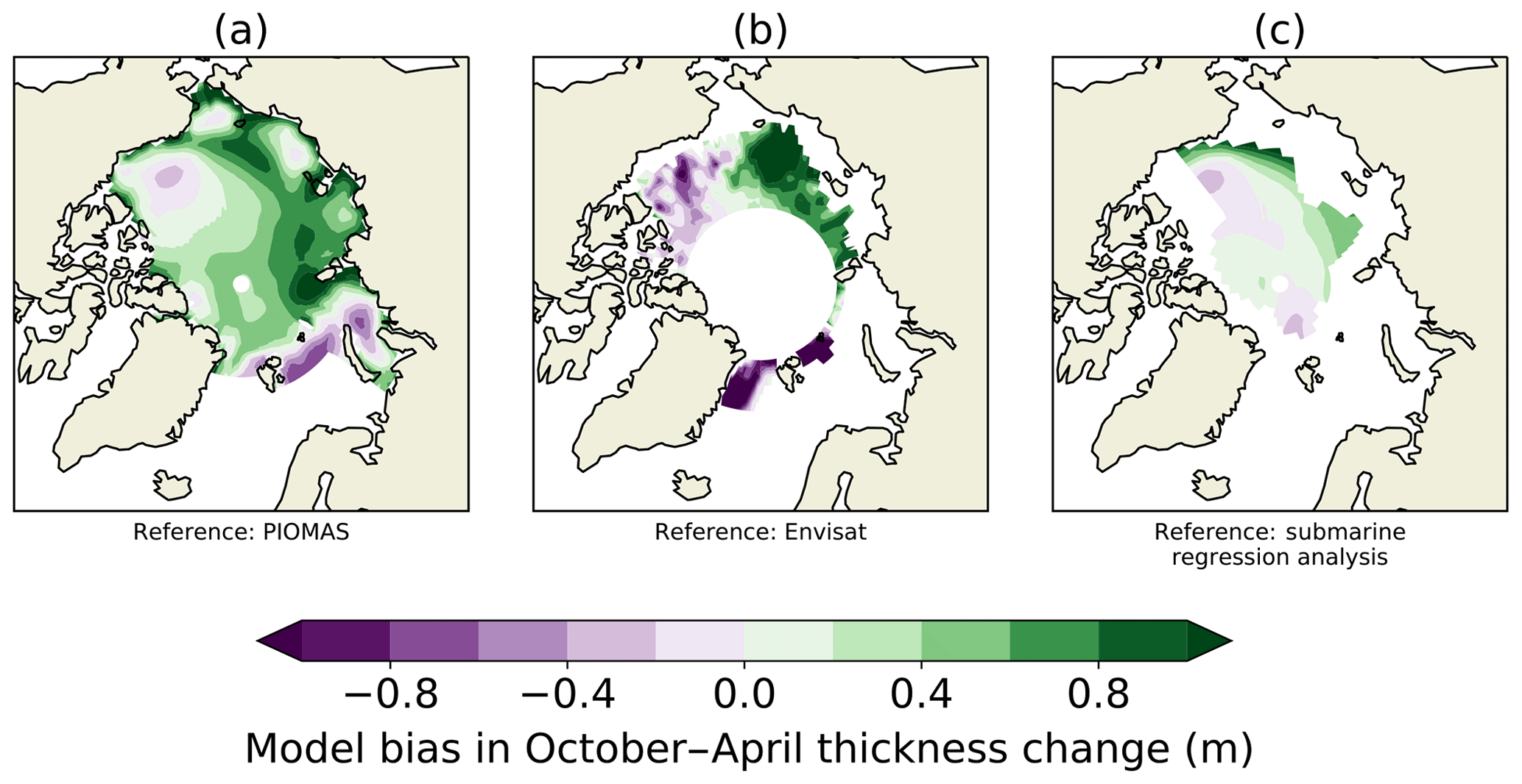
Figure 3HadGEM2-ES model bias in ice thickness change from October to April compared to (a) PIOMAS 1980–1999, (b) Envisat 1993–2000 and (c) submarine regression analysis 1980–1999. In each plot, the model period used matches the period of the reference dataset. Differences are taken as model reference so that areas of green (purple) correspond to areas where the HadGEM2-ES model simulates too much (not enough) sea ice growth through the winter.
Arctic mean ice thickness is lower than that estimated by PIOMAS for the Arctic (Fig. 2b), with the largest bias of −0.4 m in October (minimum of the annual cycle) and a near-zero bias in May close to the maximum. Modelled ice thickness is also biased low relative to the ERS satellite measurements (Fig. 2c), with biases ranging from −0.57 m in November to −0.16 m in April. Finally, modelled ice thickness is biased low relative to the submarine data (Fig. 2d), at −1.5 m in August and −0.8 m in January and May. We conclude that annual mean ice thickness is biased low in HadGEM2-ES.
There is also a model bias in the seasonal cycle of volume balance. Model biases at minimum ice thickness tend to be larger (i.e. more negative) than those at maximum ice thickness. The model simulates excess ice melt in summer, and excess ice growth in winter, equivalent to 38, 42 and 38 cm over the Arctic Ocean region on average, relative to PIOMAS, ERS altimetry and submarine upward-looking sonar, respectively (Fig. 1). Hence HadGEM2-ES is likely to overestimate the magnitude of the ice thickness seasonal cycle by around 40 cm across the Arctic Ocean on average. In particular, the large negative model bias in ice thickness in late summer is likely to be the principal cause of the low bias in the September ice area. We note that both ERS and submarine measurements are seasonally and spatially limited; in each comparison above, model data are calculated only for regions and times of year for which data exist in the respective dataset.
The thin ice thickness bias is smaller on the Pacific side of the Arctic than on the Atlantic side of the Arctic in both April and October, relative to all three datasets, becoming very small or positive in the Beaufort Sea (Fig. 2b–d). The seasonal cycle in ice thickness in HadGEM2-ES is amplified across much of the Arctic, but not in the Beaufort Sea (Fig. 3), relative to all three datasets; here, the seasonal cycle amplitude is diagnosed as the difference between April and October ice thickness. There is a correspondence between areas where modelled annual mean ice thickness is biased low (high) and areas where the modelled seasonal cycle is over-amplified (under-amplified). This is likely to be associated with the ice thickness–growth feedback, whereby a steeper temperature gradient induces stronger conduction and hence ice growth for thin ice. Indeed, negative correlations between summer sea ice and sea ice growth the following winter are a ubiquitous feature of CMIP5 models (Massonnet et al., 2018).
The bias in ice volume balance is associated with a bias in ice energy uptake. Ignoring sensible heat uptake, and assuming a constant ice density of 917 kg m−3 (as used in HadGEM2-ES), a 40 cm ice melt bias during summer is associated with an energy uptake bias of around 1.5×10⁸ J, or 15 Wm−2 over a 4-month melting season; a 40 cm ice growth bias during winter is associated with an energy uptake bias of −7.5 Wm−2 over an 8-month freezing season. The ice energy uptake has three drivers: surface energy balance, oceanic heat convergence and ice divergence. For the rest of this study, we concentrate on the surface energy balance and neglect the other two terms, although the ocean heat convergence is briefly discussed in Sect. 6. This is justified by observing that sea ice divergence is comparatively small in magnitude (e.g. Serreze et al., 2007), and that while Arctic Ocean heat convergence can be significant, across much of the Arctic the sea ice is insulated from the warm Atlantic layer beneath by fresh water derived mainly from river runoff (e.g. Serreze et al., 2006; Stroeve et al., 2012b). Hence in the Arctic Ocean interior direct solar heating of the ocean is a much larger contributor to sea ice basal melting than oceanic heat convergence, as observed by Maykut and McPhee (1995), McPhee et al. (2003) and Perovich et al. (2008), and modelled by Steele et al. (2010) and Bitz et al. (2005). In particular, oceanic heat convergence is of negligible importance to the sea ice heat budget in HadGEM2-ES (Keen and Blockley, 2018).
Surface radiative fluxes are now evaluated. In the following discussion, and throughout this study, the convention is that positive numbers denote a downwards flux. Upwelling SW radiation shows a low magnitude model bias throughout the summer (Fig. 4b), with June biases of 16, 37 and 44 Wm−2 relative to ERAI, CERES and ISCCP-FD respectively (a positive bias in an upward flux demonstrates that the modelled flux is too low in magnitude). There is no consistent signal for a low bias in downwelling SW during the summer (Fig. 4a), suggesting that the model surface albedo is biased low. Net downward SW flux shows a high model bias relative to all observational datasets in June and relative to some in July and August. Relative to CERES, the June upwelling SW bias, and hence the net SW bias, tends to be somewhat higher in magnitude towards the central Arctic (Fig. 4b–c).
The June surface albedo bias is likely to be associated with a bias in surface melt onset in HadGEM2-ES (Fig. 5). Surface melt onset, associated with the formation of low-albedo melt ponds, occurs around mid-June in the central Arctic (although earlier around the Arctic Ocean coasts), as measured by satellite observations. In contrast, HadGEM2-ES simulates surface melt onset in mid- to late May across the Arctic Ocean. This would cause a bias in surface albedo with a strong maximum in the central Arctic, consistent with the spatial pattern of the net SW bias discussed above. HadGEM2-ES parameterizes the effect of melt ponds by lowering sea ice albedo as surface temperature reaches the melting point. In the comparison to above, melt onset date in the model is defined as the first day on which the surface temperature exceeds −1 ∘C. Varying this threshold by 0.5 ∘C in either direction changes the date in only a small minority of grid cells.
LW radiation fluxes (both downwelling and upwelling) are lower in magnitude in HadGEM2-ES throughout the winter than in all observational datasets (Fig. 5d–f). For downwelling LW, the mean model biases from December to April are −16, −22 and −40 Wm−2 for ERAI, CERES and ISCCP-FD respectively. There is no indication from in situ studies as to where the true model bias may lie, as in situ studies of downwelling LW measurements have shown underestimation by CERES and overestimation by ERAI and ISCCP-FD. For upwelling LW, the biases are 11, 16 and 18 Wm−2 for CERES, ERAI and ISCCP respectively. There is uncertainty in inferring a model bias in net downwelling LW, with negative biases suggested by the satellite datasets but a neutral bias by ERAI. The bias in downwelling and net down LW is somewhat higher towards the North American side of the Arctic and lower on the Siberian side (Fig. 5d, f).
The surface radiation evaluation provides clues as to the causes of the HadGEM2-ES ice volume balance bias but also underlines why a more detailed analysis is required to properly quantify these causes. For example, in winter the low downwelling LW bias provides a clear mechanism for the bias in ice freezing. However, the reference datasets also suggest a low bias in upwelling LW that at first sight would tend to counteract this. In fact, these biases are fully consistent: a low bias in downwelling LW would be expected to cause a low surface temperature bias, causing both a high bias in ice growth and a low bias in upwelling LW. The qualitative evaluation fails to capture the full causal relationship; for this, an analysis of exactly how the downwelling LW bias affects surface flux, including the upwelling LW response, is necessary.
In the summer, meanwhile, the surface radiation evaluation suggests that a bias in net SW radiation is responsible for the ice volume balance bias, and that this in turn is related to a surface albedo bias. However, at least two possible drivers of this have been identified: the surface melt onset bias and the underlying ice area bias that is itself likely to be caused by the ice volume balance bias. Quantifying the extent to which each driver is important, and at which times of year, is likely to help in resolving this circular causal loop. In the next section, it is described how the effects of each model bias on the sea ice volume balance can be separated and quantified through their effect on the surface flux, in the ISF framework.
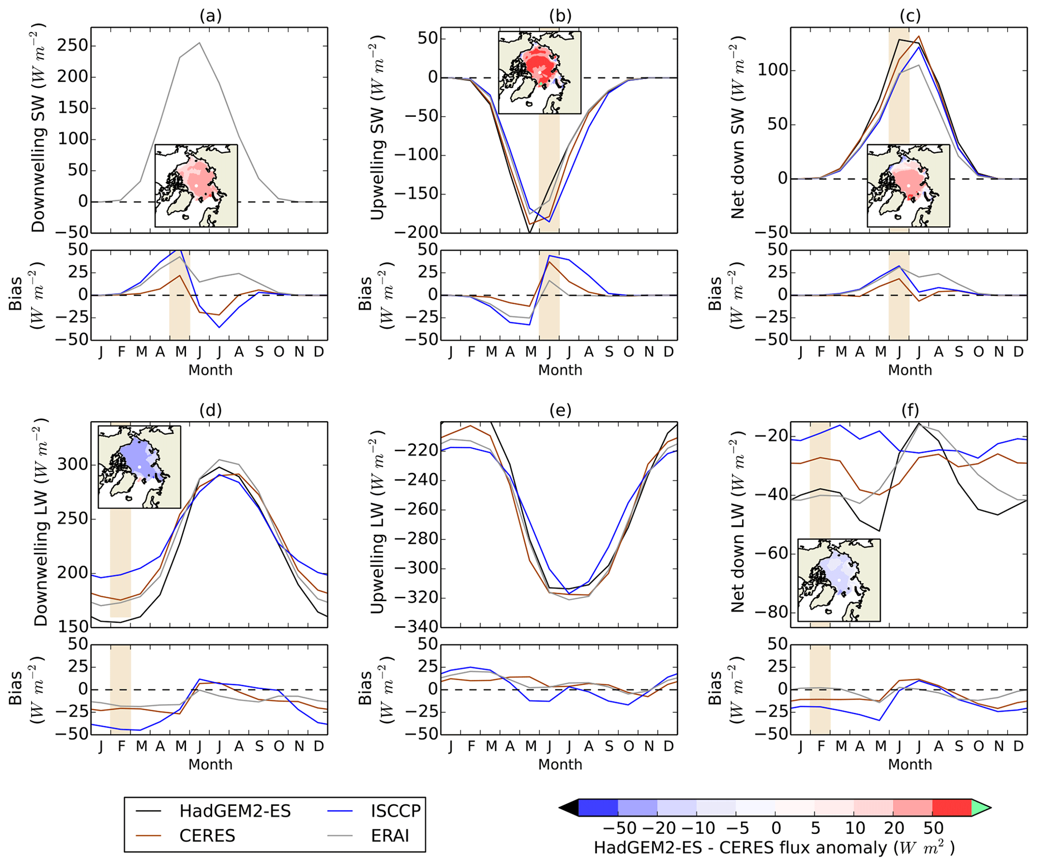
Figure 4(a) Downwelling SW, (b) upwelling SW, (c) net down SW, (d) downwelling LW, (e) upwelling LW and (f) net down LW, for HadGEM2-ES 1980–1999 over the Arctic Ocean region, compared to CERES 2000–2013, ISCCP-D 1983–1999 and ERAI 1980–1999. (a)–(c) show absolute values. (d)–(f) show model bias relative to each respective dataset. For all fluxes, a positive number denotes a downward flux and vice versa. Maps of flux bias relative to CERES are shown for downwelling SW in May, upwelling and net down SW in June, and downwelling and net down LW in February.
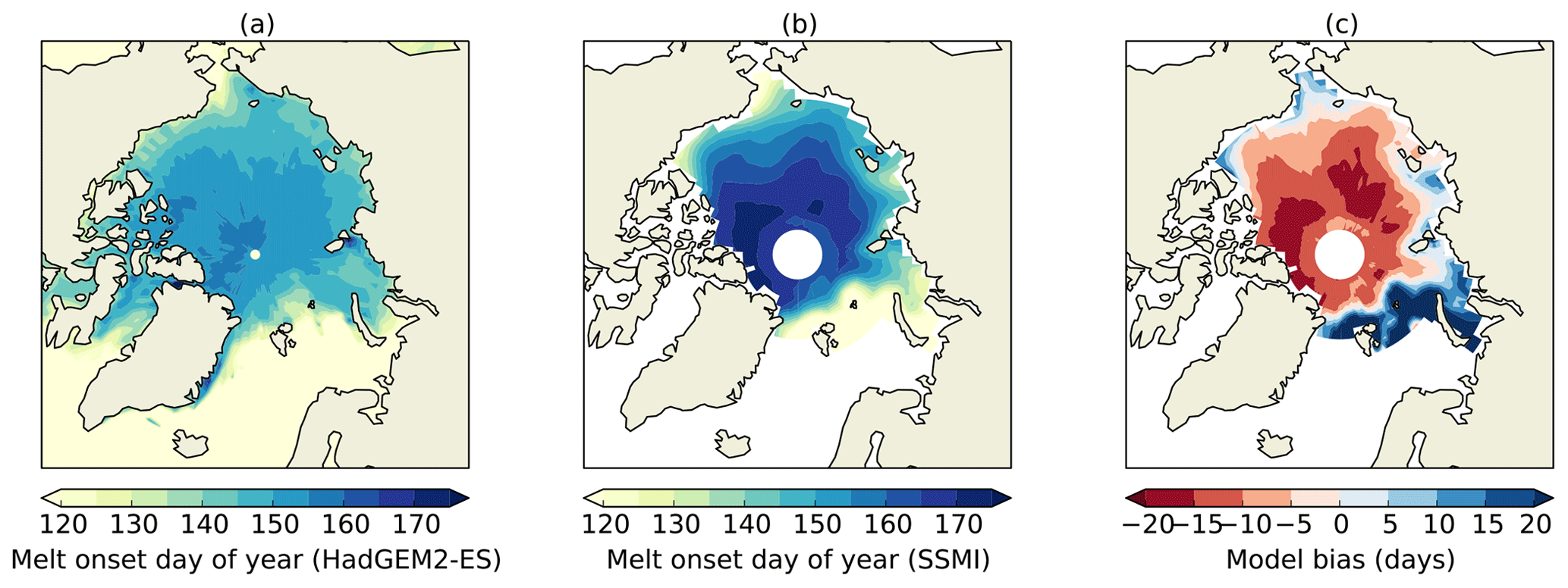
Figure 5Average date of year of surface melt onset, 1980–1999, (a) as modelled by HadGEM2-ES and (b) as measured by SSMI observations. (c) shows model bias.
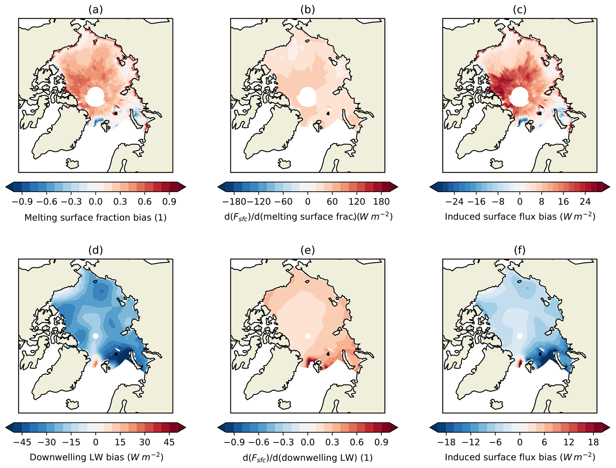
Figure 6Demonstrating the calculation of fields of surface flux bias due to model bias in melting surface fraction (a)–(c) and downwelling LW (d)–(f). (a) and (d) show model bias in each variable, (b) and (e) the local rate of dependence of surface flux on each variable as calculated above, and (c) and (f) the induced surface flux bias, calculated as the product of these two fields. The first historical simulation of HadGEM2-ES is used for the illustration.
We are motivated by the observation that each of the model biases described above affects the sea ice volume balance by acting through the total downwards surface energy flux (referred to as the surface flux). An excess of downwelling radiation leads directly to a higher surface flux, higher sea ice energy uptake and a bias towards ice melting. A bias in ice area, or in surface melt onset, is associated with a bias in surface albedo, hence a bias in net SW, and in the total surface flux. Finally, a bias in ice thickness alters the thermodynamics of the entire snow–ice column and of the near-surface atmosphere layer. Flux continuity considerations show that in the freezing season, thinner ice is associated with a warmer surface temperature, and hence a higher upwelling LW flux and a smaller total downwards surface energy flux. Thinner (thicker) ice is also associated with a stronger (weaker) upwards conduction flux and hence stronger (weaker) ice growth.
Each of these relationships can be quantified, in principle, at any point in model space and time. Specifically, the rate at which the surface flux depends on each variable alone, with others being held constant, can be estimated. To this end, we approximate the surface flux Fsfc at each point in model space x and time t by an explicit function gx,t of quasi-independent variables vi. The functions gx,t are constructed in such a way as to capture each of the relationships described above in a manner that best represents both HadGEM2-ES and also the conditions at the point x and time t. In addition, the function captures the indirect effect of any model bias on surface flux via surface temperature and upwelling LW, which will tend to counteract the direct effect to a degree. Hence the dependence of the surface flux on each of the independent variables at point x, time t can be approximated by . Given a model bias in variable vi at (x,t) we can then estimate the surface flux bias induced by that model bias as .
The function gx,t and its derivation are described fully in Appendix A but are summarized briefly here. The surface flux is expressed as a sum of separate radiative and turbulent components. Ice-covered and ice-free portions of a grid cell are treated separately; in ice-covered areas, dependence on surface temperature is linearized, and flux continuity at the surface and a uniform vertical conductive flux through the ice are assumed, allowing surface temperature to be eliminated and the dependence of surface flux on upwelling LW to be captured. The surface albedo, upon which the upwelling SW component depends, is expressed in terms of ice fraction, snow fraction and melt onset occurrence, based on the albedo parameterization of HadGEM2-ES. Latent heat flux over ice is neglected. In this way the surface flux is expressed as an explicit function of downwelling shortwave (SW) and longwave (LW) radiation, ice concentration, category ice thickness, snow thickness, sensible and latent heat fluxes over ice and ocean, and melt onset occurrence (a logical determination of whether or not the snow surface is undergoing melting). Induced surface flux due to ice thickness bias is determined by summing each of the separate ISF biases by category.
The usefulness of this approach is that surface flux operates linearly on the sea ice volume balance, meaning that each of the ISF biases at (x,t) can be averaged over large regions of time and space to understand large-scale sea ice biases. Clearly, none of the driving model biases operate on the sea ice state in a linear sense. For example, given identical surface melt onset (and hence surface albedo) biases at different points in the Arctic, each could have very different implications for local sea ice volume balance depending on the downwelling SW modelled at each point. Conversely, identical downwelling SW biases would have different implications for sea ice volume balance depending on the modelled surface albedo. Model bias in ice thickness behaves in a particularly nonlinear fashion, with bias in regions of thinner ice having far more influence than that in regions of thicker ice. The effect of estimating ISF bias at each point separately, and then averaging to determine large-scale effects, is the bypassing of all nonlinearities.
A second advantage of this approach lies in the quasi-independence of the variables. While each variable may affect the others over timescales varying from days to months, each affects the surface flux instantaneously (in HadGEM2-ES). Hence a model bias in any variable represents an effect on the surface flux that is separable from the effect of a model bias in any other. If the surface flux variation is completely described by the function gx,t, the sum of the ISF biases, over all variables, must therefore approach the true model surface flux bias (although it will be seen that this claim is impossible to evaluate precisely due to observational uncertainty). In this way, large-scale model biases in surface flux, and hence sea ice volume balance, can be broken down into separate contributions from model biases in each of the independent variables.
The ISF calculation process is now illustrated for two processes in turn. The model bias in melting surface fraction for the month of June 1980 is positive over most of the Arctic, although only weakly so towards the coasts (Fig. 6a), reflecting melt onset modelled earlier than observed during this month. The reference dataset is derived from SSMI microwave observations. The rate of change of surface flux with respect to melt onset occurrence tends to be higher in the central Arctic (Fig. 6b). This reflects a greater tendency towards clear skies in the central Arctic, as this field is effectively downwelling SW multiplied by the difference in parameterized albedos. The product of these two fields represents the modelled surface flux bias induced by the model bias in melt onset; this is also positive over most of the Arctic Ocean, by up to 25 Wm−2 in the central Arctic, reflecting the greater absorption of SW radiation induced by the early melt onset (Fig. 6c)
The model bias in downwelling LW radiation in February 1980 is predominantly negative (Fig. 6d); here CERES-EBAF is the reference dataset. The rate of dependence of surface flux on downwelling LW (Fig. 6e) is everywhere between 0 and 1, tending to be lower in regions of thicker ice, and is associated with a greater tendency for downwelling LW biases to be counteracted by upwelling LW biases in these regions. The resulting ISF bias (Fig. 6f) is negative almost everywhere but is lower in magnitude than the driving downwelling LW bias.
5.1 Aggregate ISF biases
We calculate surface flux biases induced by model biases in downwelling SW, downwelling LW, ice area, local ice thickness and surface melt occurrence (the variables for which reference datasets are available). The resulting fields are averaged over the model period and over the Arctic Ocean region, to produce for each variable a seasonal cycle of total surface flux bias induced by the bias in that variable. The induced surface flux (ISF) biases are displayed in Fig. 7 together with total ISF bias, net radiative flux bias estimated by the direct radiation evaluation relative to ISCCP-FD, CERES and ERAI, and also sea ice energy uptake biases implied by the seasonal ice volume balance bias relative to PIOMAS. The ISF biases are also shown in Table 1, using CERES as reference dataset for the radiative terms. During winter, ISF biases generally sum to negative values, indicating that model biases in this season induce net additional surface energy loss and ice growth. During summer, ISF biases generally sum to positive values, indicating additional net surface energy gain and ice melt. In both seasons, these results are consistent with the radiation and ice volume balance evaluation.

Figure 7Surface flux bias induced by model biases in ice fraction, melt onset occurrence, ice thickness, downwelling SW and downwelling LW respectively for the Arctic Ocean region in HadGEM2-ES, 1980–1999. Total ISF bias is indicated by black bars. For each month, induced surface flux biases are estimated using in turn CERES, ISCCP-FD and ERAI as radiation reference datasets, from left to right. Sea ice latent heat flux uptake bias relative to PIOMAS is indicated in black. Net radiative flux biases relative to CERES, ISCCP-FD and ERAI are indicated in brown. Spatial patterns of induced surface flux bias for four processes in key months, with CERES as reference dataset, are displayed beneath and above (© Crown copyright 2019. Distributed under the Creative Commons Attribution 4.0 License.).
Table 1Surface flux biases induced by model bias in five different variables in HadGEM2-ES (Wm−2), with CERES used as reference dataset for the radiative components. Total ISF bias and total net radiative flux bias relative to CERES are shown for comparison, as well as their residual. The difference between net radiative flux bias as evaluated by CERES and ERAI is also shown. A positive number denotes a downwards flux, and vice versa.
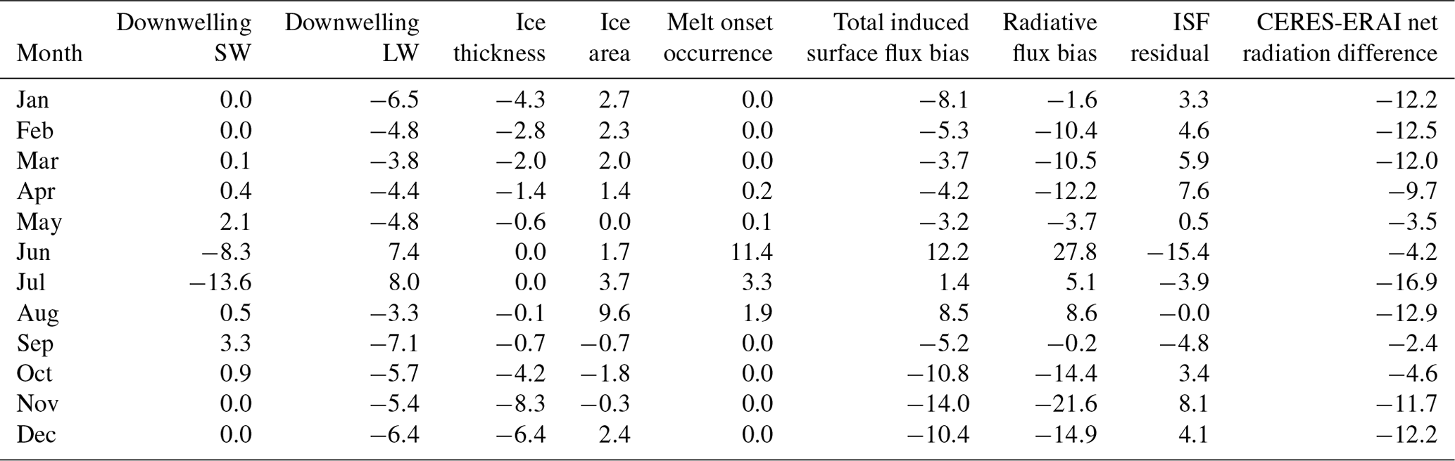
Major roles are identified for particular processes in certain months. Firstly, in June the surface melt onset bias, through its effect on the surface albedo, induces a surface flux bias of −13.6 Wm−2, equivalent roughly to an extra 11 cm of melt. Secondly, in August a bias in ice fraction induces a surface flux bias of 9.6 Wm−2, equivalent to an extra 8 cm of melt. This is associated with the overly fast retreat of sea ice in HadGEM2-ES and the low extents in late summer, as noted in Sect. 3. Thirdly, from October to March the downwelling LW biases induce substantial surface flux biases ranging from −6.5 to −3.8 Wm−2 depending on choice of reference dataset, equivalent to additional sea ice growth of 20–33 cm. Finally, from November to March the negative ice thickness bias induces substantial surface flux biases reducing from −8.3 to −2.0 Wm−2 as the freezing season progresses and is equivalent to a total additional ice growth of 24 cm.
Internal variability in the ISF biases is measured by taking the standard deviation of the whole-Arctic ISF bias for each process and month across all 20 years in the model period, and all four ensemble members used. Variability is highest in the ice area term, reaching 4.0 Wm−2 in July. Variability reaches considerable size in some other terms in some months, for example 1.1 Wm−2 for surface melt onset in June, 1.9 Wm−2 for ice thickness in November but is otherwise mainly under 1 Wm−2 in magnitude. In each case, therefore, the ISF biases noted above are persistent features of the model; surface melt onset and ice fraction biases induce additional ice melt in summer, while downwelling LW and ice thickness biases induce additional ice growth in winter. The total summer volume balance bias accounted for by the analysed processes is of the order 20 cm, while the total winter volume balance bias is of the order 45–55 cm depending on radiation reference dataset.
5.2 Spatial variability
Examining first the June melt onset ISF bias, the spatial pattern of the bias is characterized by a maximum in the central Arctic, with values falling away towards the coast; this is directly related to the spatial pattern of the melt onset bias itself shown in Fig. 6. It is very similar to the spatial pattern of the directly evaluated net SW bias in this month, providing additional evidence that the melt onset bias is the principal cause of this. This implies that the additional ice thinning induced by this bias is greatest in the central Arctic and least at the coasts.
The August ice concentration ISF bias displays a sharply defined pattern, with high values across the shelf seas and the Atlantic side of the Arctic falling to low or negative values in the Beaufort Sea, again very similar to the pattern of the ice concentration bias itself. The implication is that the model bias towards ice thinning in August is largely based in areas where ice concentration is already biased low.
The November–March ice thickness ISF bias displays a pattern which is almost identical to that of the August ice fraction ISF bias, but with the opposite sign, with high negative values on the Atlantic side of the Arctic rising to near-zero values in the Beaufort Sea. Hence this model bias has the reverse effect to that of the ice concentration bias, reducing existing ice thickness biases by promoting additional ice growth in these areas.
Finally, the winter downwelling LW ISF bias is much more spatially uniform but displays slightly higher values on the Pacific side of the Arctic than the Atlantic side, which is a different pattern to that displayed by the downwelling LW itself in Fig. 4d. The contrast is due to the role the effective ice thickness scale factor plays in determining the induced surface flux bias; the thicker ice present on the American side of the Arctic tends to greatly reduce the flux bias. This represents the thickness–growth feedback; thicker ice will grow less quickly than thin ice under the same atmospheric conditions. The downwelling LW bias tends to increase ice growth Arctic-wide but less so in regions where ice is already thick.
The spatial patterns of total ISF bias show many similarities to the total net radiation bias evaluated by CERES in most months of the year (Fig. 8). Notably there is a tendency in July and August for positive surface flux biases to be concentrated on the Atlantic side of the Arctic, and a tendency throughout the freezing season for negative surface flux biases to be least pronounced in the Beaufort Sea, where the ice thickness biases are lowest. We note that the spatial pattern of amplification of the ice thickness seasonal cycle displayed in Fig. 3 is very similar, with amplification most pronounced in the Atlantic sector and least pronounced in the Beaufort Sea. The surface flux biases produced by ice fraction biases in August, and ice thickness biases in November, provide reasons for the spatial variation in amplification of the ice thickness seasonal cycle seen in Fig. 4, as well as the close resemblance of this pattern to the model biases in annual mean ice thickness. Ice which is thinner in the annual mean will tend to melt faster in summer, due to the net SW biases associated with greater creation of open water (the surface albedo feedback) and will tend to freeze faster in winter, due to greater conduction of energy through the ice (the ice thickness–growth feedback).

Figure 8Comparing fields of total ISF bias (left) to net radiation bias (right) relative to CERES for each month of the year for the four historical members of HadGEM2-ES, 1980–1999.
5.3 Using the ISF biases to separate sea ice forcings and feedbacks
It is helpful to divide the processes examined into feedbacks (surface flux biases induced by biases in the sea ice state itself) and forcings (those induced by variables external to the sea ice state). In this sense, a “forcing” refers to a variable which is independent of the sea ice volume on instantaneous timescales, rather than being used in the traditional sense of a radiative forcing. Of the variables examined, downwelling SW and LW radiation, as well as the surface melt onset, have this property, and hence their corresponding ISF biases can each be regarded as a “forcing” on the sea ice state. However, ice thickness and area do not have this property, and their corresponding ISF biases should be regarded instead as intrinsic feedbacks of the sea ice state.
The ice concentration ISF flux bias (specifically during the melting season) can be identified with the effect of the surface albedo feedback on the sea ice state. During the melting season the ice area affects the estimated surface flux only through the surface albedo, and the surface flux biases induced in this way cause associated biases in ice melt.
On the other hand, the ice thickness ISF bias (specifically during the freezing season) can be identified with the effect of the thickness–growth feedback on the sea ice state. This is perhaps less obvious, as the ice thickness affects the estimated surface flux via the surface temperature and upwelling LW radiation, while the thickness–growth feedback is usually understood to result from differences in conduction. However, the assumption of flux continuity at the surface in constructing the estimated surface flux means that the cooler surface temperatures, and shallower temperatures gradients occurring for thicker ice categories are manifestations of the same process. Slower ice growth at higher ice thicknesses is caused by a smaller negative surface flux, and the surface temperature is the mechanism by which this is demonstrated. Hence the effect of the thickness–growth feedback is described by the ice-thickness-induced component of the surface flux bias.
The ISF analysis allows the effect of the surface albedo and thickness–growth feedbacks on the sea ice state to be quantified and compared to the effect of external drivers. Arctic-wide, the surface albedo feedback, diagnosed as the ice-area-induced component of the surface flux bias, contributes an average of 5.2 Wm−2 to the surface flux bias over the summer months, equivalent to an extra 13 cm of ice melt. This is very similar to the effect of the component induced by the surface melt onset, which contributes an average of 5.3 Wm−2, equivalent also to an extra 13 cm of ice melt. In the freezing season, meanwhile, the thickness–growth feedback, diagnosed as the ice-thickness-induced component of the surface flux bias, contributes an average of −4.4 Wm−2 to the surface flux bias from October to April, equivalent to an extra 26 cm of ice freezing, while the downwelling-LW-induced component (using CERES as reference dataset) contributes an average of −4.9 Wm−2, equivalent to an extra 29 cm of freezing over this period.
5.4 ISF residuals and observational uncertainty
The ISF biases, summed over all independent variables, should approach the true total surface flux bias. However, this is difficult to evaluate as the true surface flux bias is not known. Hence it is necessary to use proxy quantities to evaluate the total ISF bias. We use directly evaluated surface net radiation bias (relative to ISCCP-FD, ERAI and CERES respectively), and ice energy uptake bias, derived from ice volume balance bias relative to PIOMAS.
For most months of the year, all estimates of total ISF bias fall within the spread of these four datasets (Fig. 6), the exceptions being June and July when total ISF bias is smaller than all surface flux proxies. However, the spread is extremely large. For example, in the month of January the estimates of total ISF bias are −12.3, −8.2 and −6.1 Wm−2 (with ISCCP-FD, CERES and ERAI used as downwelling radiation datasets respectively), while the estimates of net radiation bias are −18.2, −11.6 and 0.6 Wm−2 from ISCCP-FD, CERES and ERAI respectively, and ice heat uptake bias is estimated as −10.1 Wm−2. Hence it is difficult to evaluate the total ISF bias within current observational constraints, and at best it can be said that the total ISF bias is qualitatively consistent, over the year as a whole, with the surface flux bias proxies. A possible cause of the lower total ISF bias in June and July is the “missing process” of snow on ice, which cannot be evaluated here due to the lack of a reference dataset. The early surface melt onset, and sea ice fraction loss, as modelled by HadGEM2-ES, would be associated with an early loss of snow on ice, with an additional surface albedo bias and hence an additional ISF bias.
On the other hand, the annual mean ice heat uptake bias (0.0 Wm−2) provides a strong constraint on the annual mean surface heat flux bias in the absence of a significant oceanic heat convergence contribution. For example, the annual mean total ISF biases are −3.6 and −4.5 Wm−2 when CERES and ISCCP-FD are used as reference datasets respectively; these would imply sea ice thickening of 7 and 9 m over the 1980–1999 in HadGEM2-ES, which does not occur. Hence in the annual mean, the total ISF bias is too low. This annual mean bias is related to the tendency for the ISF analysis to account for a greater bias towards ice growth in winter (45–55 cm) than that towards ice melt in summer (20 cm). It is likely to be derived, at least in part, from the use of multiple reference datasets whose errors are not constrained to correlate in a physically realistic sense but may also be related to the missing processes in June and July.
Observational error is one potential cause of error in the ISF biases. An idea as to the potential magnitude of this can be seen from the large spread in SW and LW ISF bias (across different datasets) during summer (Fig. 6). For example, in July the model downwelling LW bias with respect to ERAI produces an aggregated ISF bias of −7.0 Wm−2, but that with respect to CERES produces an aggregate ISF bias of 8.0 Wm−2. Calculation of ice area ISF biases using NSIDC and HadISST.2 as references, described in Sect. 2.2 and not shown here, showed a similar magnitude of uncertainty in the ice area term (±10 Wm−2 in summer, ±2 Wm−2 in winter). We note that the evidence from in situ validation studies suggests that the winter downwelling LW estimates of ERAI and CERES are more likely to be accurate than that of ISCCP-FD. Hence the downwelling LW ISF bias is likely to be estimated more accurately when ERAI or CERES are the reference dataset, and the bias towards ice growth is likely to lie closer to the lower end of the range (20 cm).
In Appendix B, inherent theoretical errors in the ISF analysis are discussed and are found to be small relative to the sensitivity to use of observational datasets. The largest errors are listed here: firstly, due to sub-monthly variation in the component variables, the winter downwelling LW component may be underestimated in magnitude by around 0.6 Wm−2 on average, and the ice area component in August may be overestimated by around 1.6 Wm−2. Secondly, due to the evaluation of surface flux dependence at a model state which is itself biased, the total ISF bias in October is overestimated in magnitude by around 3.6 Wm−2. Thirdly, due to nonlinearities in the surface flux dependence on ice thickness, the ice thickness component is overestimated in magnitude by 0.7 Wm−2 on average from October to April, with a maximum overestimation in November of 1.9 Wm−2. As these biases are, in the main, considerably smaller than the differences between ISF biases when different reference datasets are used, it is concluded that observational errors are the more important contribution to error in the ISF biases.
6.1 Using the ISF framework to understand the HadGEM2-ES sea ice state
The HadGEM2-ES ISF biases are qualitatively consistent with the direct net radiation evaluation and with the sea ice simulation, both in terms of seasonal and spatial variation, and allow the effect of the surface albedo feedback and thickness–growth feedback on the sea ice volume balance to be separated. This allows the HadGEM2-ES sea ice biases to be understood by considering, in turn, the separate ISF components, their magnitudes, and the times of year when they are important. The anomalous summer sea ice melt is initiated by the early melt onset occurrence and maintained by the surface albedo feedback, which acts preferentially in areas of thinner ice. The anomalous winter ice growth is maintained both by the thickness–growth feedback (occurring mainly in areas of thinner ice, of greater importance in early winter) and by the downwelling LW bias (more spatially uniform, in late winter). It is unclear that any significant role is played by the downwelling SW bias, as at the only time of the year when the radiation datasets agree that this bias is of significant value (May), the induced surface flux bias is more than balanced by that induced by downwelling LW. However, this may have a role in causing the later melt onset bias, as discussed below.
The means by which the external forcings – anomalous LW winter cooling and early late spring melt onset – cause an amplified seasonal cycle in sea ice thickness are clear. It can also be seen how, in the absence of other forcings, these combine to create an annual mean sea ice thickness that is biased low, as seen in Sect. 4. The melt onset forcing, by inducing additional ice melting through its effect on the ice albedo, enhances subsequent sea ice melt through the surface albedo feedback. The downwelling LW bias, on the other hand, by inducing additional ice freezing through its cooling effect attenuates subsequent sea ice freezing through the thickness–growth feedback. Surface flux biases induced by melt onset occurrence are enhanced, while those induced by downwelling LW are diminished.
Acting together, the ice thickness–growth feedback and surface albedo feedback create a strong association between lower ice thicknesses and amplified seasonal cycles, because ice which tends to be thinner will both grow faster during the winter and melt faster during the summer. Hence the melt onset bias, acting alone, would induce a seasonal cycle of sea ice thickness whose annual mean thickness is lower, but that was also more amplified than that observed. This is because the surface albedo and thickness–-growth feedbacks act to translate lower ice thicknesses into faster melt and growth. For similar reasons, the downwelling LW bias, acting alone, would induce a seasonal cycle of sea ice thickness whose annual mean thickness is higher, and that was also less amplified than that observed.
The bias seen in HadGEM2-ES is a result of the melt onset bias “winning out” over the downwelling LW, due to it occurring at a time of year when the intrinsic sea ice feedbacks render the ice far more sensitive to surface radiation. The anomalously low ice cover in September arises as a consequence of the low annual mean ice thickness and in particular as a consequence of the anomalously severe summer ice melt. The finding that the low annual mean ice thickness is driven by surface albedo biases is consistent with the finding by Holland et al. (2010) that variance in the mean sea ice volume in the CMIP3 ensemble was mostly explained by variation in summer absorbed SW radiation.
The feedbacks of the sea ice state explain the association between spatial patterns of annual mean ice thickness bias and ice thickness seasonal cycle amplification. However, the external forcings (melt onset and downwelling LW bias) cannot entirely explain the spatial patterns in the mean sea ice state biases, because on a regional-scale effects of sea ice convergence, and hence dynamics, become more important. The annual mean ice thickness bias seen in HadGEM2-ES is associated with a thickness maximum on the Pacific side of the Arctic, at variance with observations which show a similar maximum on the Atlantic side. It was shown by Tsamados et al. (2013) that such a bias could be reduced by introducing a more realistic sea ice rheology.
6.2 Looking beyond proximate drivers
The ISF framework, as noted in Sect. 1, can only identify the proximate causes of sea ice biases. Here, we briefly discuss causes of the two external drivers. Underestimation of wintertime downwelling LW fluxes in the Arctic is known to be a widespread model bias in the CMIP5 ensemble (e.g. Boeke and Taylor, 2016) probably associated with cloud liquid water deficit caused by errors in cloud microphysics schemes (Pithan et al., 2014). HadGEM2-ES was not one of the models assessed by Pithan et al. (2014), but its winter climate simulation displays many of the characteristic CMIP5 biases, namely low cloud liquid water fractions during winter compared to MODIS observations (Fig. 9a). In addition, observations suggest a bimodal nature of Arctic winter temperatures associated with strong and weak inversions, (e.g. Stramler et al., 2011; Raddatz et al., 2014), and a failure to simulate the milder mode (Fig. 9b), diagnosed by 6-hourly fluxes of net LW, is a feature of the HadGEM2-ES simulation similar to the models assessed by Pithan et al. (2014). Here we conclude that a similar mechanism is likely to be at work in HadGEM2-ES and that insufficient cloud liquid water is the principal driver of the anomalously low downwelling LW fluxes.
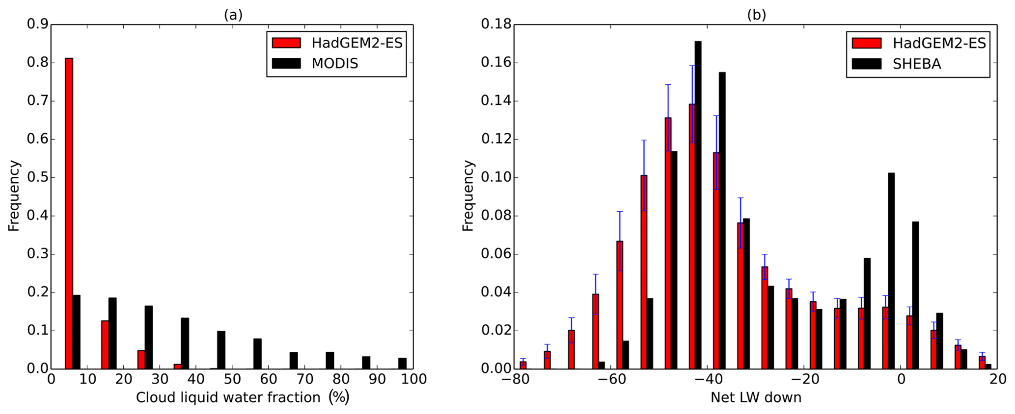
Figure 9Frequency distributions of (a) October–April cloud liquid water percentage in HadGEM2-ES compared to MODIS observations, for the Arctic Ocean region. (b) December–February surface net downwelling LW in HadGEM2-ES in the SHEBA region, compared to the values observed at SHEBA.
The causes of the early melt onset bias of HadGEM2-ES are harder to determine. For most of the spring, comparisons of daily upwelling LW fields of HadGEM2-ES to CERES-SYN observations (not shown) show the Arctic surface to be anomalously cold in the model, as during the winter. During May, however, upwelling LW values rise much more steeply in the model, and surface melt onset commences during mid-to-late May, far earlier than in the satellite observations. A possible cause of the overly rapid surface warming during May is the zero-layer thermodynamics approximation used by HadGEM2-ES, in which the ice heat capacity is ignored. Comparing fields of surface temperature in HadGEM2-ES between the beginning and the end of May shows a “missing” ice sensible heat uptake flux of 10–30 Wm−2 over much of the central Arctic, which would in turn be associated with a reduction of flux into the upper ice surface of 5–15 Wm−2. Examination of modelled and observed daily time series of downwelling LW and net SW fluxes in late May and early June suggests that a surface flux reduction of this magnitude could delay surface melt by up to 2 weeks. This would represent a substantial part of the modelled melt onset bias seen.
Another cause of the rapid warming may be the increasing relative magnitude of the downwelling SW response to cloud biases, as May progresses (compared to the downwelling LW response). Comparison of 5-daily means of HadGEM2-ES radiative fluxes during May to those from the CERES-SYN product (not shown) supports this hypothesis; a modelled bias in downwelling SW grows quickly during early May, from ∼0 to ∼30 Wm−2, while the modelled bias in downwelling LW remains roughly constant.
6.3 Missing processes in the ISF analysis
The ISF analysis, as presented, does not comprise an exhaustive list of processes affecting Arctic Ocean surface fluxes. The missing process of the effect of snow fraction on surface albedo, and its likely effect on the total June and July ISF bias, has already been noted. We note also that the direct effect of thinning ice on ice albedo could induce an additional flux bias relative to the real world, despite the fact that this effect is not represented in HadGEM2-ES. The effect of snow thickness bias on winter conduction and surface temperature is another such process which cannot be included due to inadequate observations. Model biases in the turbulent fluxes may also be significant. While the process which is likely most important in determining these during the winter is captured (ice fraction in the freezing season), a more detailed treatment of turbulent fluxes would also examine the effect on these of the overlying atmospheric conditions. It is also noted that snowfall itself is a component of the surface flux that could, in theory, be evaluated directly given a sufficiently reliable observational reference.
A complete treatment of model biases affecting the sea ice volume budget would also examine causes of bias in oceanic heat convergence. For the reasons discussed in Sect. 4, these are likely to be small in the Arctic Ocean interior in HadGEM2-ES and in observations, but the model bias could nevertheless conceivably be of considerable size in the context of the surface flux biases shown in Fig. 6. The total Arctic Ocean heat convergence modelled by HadGEM2-ES for the period 1980–1999 is 4.4 Wm−2, although this figure shows high sensitivity to the location of the boundary in the Atlantic sector, suggesting that most of this heat is released close to the Atlantic ice edge. This figure is slightly higher than the 3 Wm−2 found by Serreze et al. (2007) in their analysis of the Arctic Ocean heat budget but is broadly consistent with observational estimates of oceanic heat transport through the Fram Strait from 1997 to 2000 by Schauer et al. (2004) (likely to be the major contributor to Arctic Ocean heat convergence). This suggests that errors in oceanic heat convergence are unlikely to contribute significantly to sea ice volume biases in HadGEM2-ES. However, for a hypothetical model that simulated greater oceanic heat convergence in the Arctic Ocean interior, the surface flux analysis presented here would fail to adequately describe the model bias in the sea ice volume budget.
Finally, the assumptions underpinning the ISF framework include an instantaneous effect of the independent variables on the surface flux. In the real world, and in many models, there is a time lag associated with the effect of the ice and snow thickness, due to the thermal inertia of the snow and ice. In the time taken for a change of ice thickness to cause a change in surface flux, other variables such as downwelling radiation could in theory be affected, raising doubts as to whether ice and snow thickness are truly independent variables. However, it is likely that any mechanism by which ice thickness could affect another variable would act first through the surface flux, and hence that the timescale on which ice thickness affects surface flux is shorter than that on which it affects other variables. It is also seen in this study that the ISF biases are largest, by far, in the thinnest ice category, where the effect of ice thickness on surface flux would be near instantaneous. ISF biases in the thickest ice category, where the time lag could be of significant size, tend to be negligible.
A framework has been designed (the ISF framework) that allows the proximate causes of biases in sea ice volume balance to be separated and quantified. Given reference datasets for independent variables, fields of induced surface flux bias can be calculated from the underlying model bias; these in theory sum to the total surface flux bias. In practice, the total ISF bias matches both the net radiation bias, and the ice volume balance bias to the first order. Processes evaluated cause around 40 cm additional ice growth during the ice freezing season and 20 cm additional ice melt in winter; a missing process for which we have no reference (snow thickness) is likely to account for at least some additional ice melt in summer. However, observational uncertainty in the evaluated terms prevents direct evaluation of the total ISF bias and is the largest contribution to ISF uncertainty.
The ISF analysis enables model biases in sea ice growth and melt rate to be attributed in detail to different causes. In particular, the roles played by the surface–albedo feedback, by the sea ice thickness–growth feedback and by external forcings can be quantified. The analysis reveals how the melt onset bias of HadGEM2-ES tends to make model ice thickness both low in the annual mean and too amplified in the seasonal cycle, with the downwelling LW bias acting to mitigate both effects. The result is consistent with the prediction of DeWeaver et al. (2008) that sea ice state is more sensitive to surface forcing during the ice melt season than during the ice freeze season. The analysis also suggests that through an indirect effect on surface albedo at a time when sea ice is particularly sensitive to surface radiation biases, the zero-layer approximation, which was until recently commonplace in coupled models, may be of first-order importance in the sea ice state bias of HadGEM2-ES.
The ISF analysis also allows a more detailed analysis of the spatial patterns in sea ice volume balance simulation. In particular, the mechanisms behind the near-identical spatial pattern of biases in annual mean ice thickness (likely driven by ice dynamics) and that of biases in the ice volume balance are explicitly demonstrated. Where ice thickness is biased low in the annual mean, an enhanced seasonal cycle is apparent. This is due to the ice thickness ISF bias (in the freezing season) and the ice area ISF bias (in the melting season), corresponding to the thickness–growth and ice albedo feedbacks. The downwelling LW and melt onset biases, by contrast, are more spatially uniform and do not contribute to the annual mean ice thickness control on the ice volume balance.
The finding that observational uncertainty is the most important cause of uncertainty in the ISF bias calculation itself suggests that if observational uncertainty could be reduced, the ISF analysis could become a very powerful tool for Arctic sea ice evaluation. In particular, large observational uncertainties for snow cover and summer surface radiation limit the overall accuracy of the methodology presented here. The addition of freezing season snow thickness, and melt season snow fraction, would represent useful extensions to the analysis presented. An additional caveat is that the ISF framework does not consider factors influencing turbulent fluxes (with the exception of the ice area, but this contribution is subject to particularly high uncertainty). It also does not consider the influence of oceanic heat convergence on sea ice state; in HadGEM2-ES the latter is small (∼10 %) but might be more significant in other models.
The ISF analysis, as presented here, is designed specifically to approximate HadGEM2-ES but could in principle be generalized to other models, particularly by altering the surface albedo parameterization used here or by using different sea ice thickness categories. The zero-layer thermodynamic assumption used in the ISF analysis is likely to be appropriate for any model during the ice freezing season, as the largest ISF biases tend to arise from the thinnest ice categories, in which the zero-layer approximation is closest to reality. However, there is a question as to whether the zero-layer approximation conceals significant surface flux bias relating to ice sensible heat uptake in the late spring.
In the case study presented here, the analysis provides mechanisms behind a model bias in sea ice simulation. However, the analysis could also be used to investigate a sea ice simulation that was ostensibly more consistent with observations, to determine whether or not the correct simulation was the consequence of model biases that cause opposite errors in the surface energy budget; a negative result would greatly increase confidence in the future projections of such a model. The analysis could be also used to investigate a model ensemble, to attribute spread in modelled sea ice state to spread in the underlying processes affecting the SEB, focussing attention on ways in which spread in modelled sea ice could be reduced. It is noteworthy that Shu et al. (2015) found the CMIP5 ensemble mean Arctic sea ice volume to be biased low in its annual mean, and over-amplified in its seasonal cycle, relative to PIOMAS (albeit over the entire Northern Hemisphere), suggesting that the behaviour exhibited by HadGEM2-ES may be quite common in this ensemble.
Finally, it is suggested that the ISF framework, as well as being used to compare a model to observations, could also be used to understand the reasons for the biases of one model with respect to another. Such a comparison would avoid the issues of observational uncertainty discussed above, enabling the contributions of the different model variables to the surface flux biases to be evaluated more accurately. However, the choice as to which model parameters on which to base the ISF framework would be subjective.
The ISF framework depends upon the construction, at each point in the model space and time, of an explicit function gx,t, which approximates the surface flux as a function of quasi-independent variables vi. The functions gx,t are constructed as follows. We start from the standard equation for surface flux:
where the surface flux is expressed as the sum of separate radiative and turbulent components. In this equation, αsfc represents surface albedo, FSW↓ downwelling SW flux, FLW↓ downwelling LW flux, εsfc=0.98 ice emissivity (as parameterized in HadGEM2-ES), Wm−2 K−4 (the Stefan–Boltzmann constant), Tsfc surface temperature, Fsens sensible heat flux, Flat latent heat flux and Fsnowfall heat flux represented by the transfer of negative enthalpy from the atmosphere to the ice associated with snowfall.
Given a model grid cell x, over a model month t, the cell is classified as freezing or melting depending upon whether the monthly mean surface temperature is greater or lower than −2 ∘C. In the case that the cell is classified as melting, Eq. (A1) is simplified in the following way: Tsfc=Tf, where Tf=0 ∘C, and Fsnowfall and Flat are both neglected. In addition we expand
where aice is ice concentration, αice mean surface albedo over sea ice and αocn=0.06 the albedo of open water used by HadGEM2-ES. Finally the ice albedo is further expanded.
Here αsea=0.06, αmelt_ice=0.535, αmelt_snow=0.65, αcold_ice=0.61 and αcold_snow=0.8 denote the parameterized albedos of open water, melting ice, melting snow, cold ice and cold snow respectively, and γmelt denotes melting surface fraction as a fraction of ice area, while Isnow is an indicator for the presence of snow that is set to 1 or 0 depending on whether monthly mean snow thickness exceeds 1 mm. Equation (A3) mimics the parameterization of ice albedo in HadGEM2-ES, in which the albedo of both snow and ice is progressively reduced from the “cold” to the “melting” values as surface temperature rises from −1 to 0 ∘C.
If the grid cell is classified as freezing, we likewise ignore Fsnowfall. We assume FSW↓ and FLW↓ to be constant across a grid cell, and parameterize αsfc as above. We expect the remaining terms (, Fsens and Flat) to vary over the six different surface types present in a grid cell: open water and the five different ice thickness categories. Hence we express each as a sum over the surface types as follows:
We make the following further approximations: firstly, that for all ice categories; secondly, that for all categories (i.e. that the sensible heat flux does not vary across categories); thirdly, that ∘C. Lastly, for each ice category we approximate , where and , and Tsfc−REF being the monthly mean surface average temperature of the grid cell x.
Flux continuity implies that over each category the surface flux is equal to Fcondtop−cat, the downwards conductive flux from the ice surface, unless surface melting is taking place; as the freezing case is being discussed, melting is assumed to be zero. We also make the zero-layer approximation used in HadGEM2-ES, that the sea ice has no sensible heat capacity and that conduction is therefore uniform in the vertical for each category. This implies that
where ∘C is ice base temperature and , with kice and ksnow being ice and snow conductivity respectively, and hice−cat and hsnow local ice and snow thickness (the latter of which is assumed to be uniform across ice categories). For each category, setting allows Tsfc−cat to be eliminated. This results in the following equation for Fsfc:
where
and
Hence we approximate the surface flux as a function of ice area, category ice thickness, snow thickness, downwelling SW, downwelling LW, melting surface fraction, sensible heat fluxes over ice and open water, and latent heat flux over open water. In the ISF analysis, we analyse the resulting dependence of surface flux on ice area, ice thickness, melting surface fraction, and downwelling SW and LW, all of which in HadGEM2-ES affect the surface flux instantaneously and can therefore be said to be quasi-independent.
Ice thickness does not appear in the surface flux formula directly; instead, the surface flux is expressed as a function of the individual category thicknesses hice−cat. To estimate the ISF bias due to ice thickness, it is hence necessary to sum over categories the ISF biases due to bias in each hice−cat. The estimation of model biases in hice−cat, therefore, requires some discussion.
Given an estimated model bias in mean thickness , it can be argued that the least arbitrary approach is to estimate the model bias in each thickness category to also be (i.e. the thickness distribution is uniformly shifted to higher or lower values). However, this leads to unphysical results at the low end of the distribution. In the case of a negative bias, it implicitly assumes the creation of sea ice of negative thickness, and in the case of a positive bias, it assumes that no sea ice of thicknesses between 0 m and exists.
Hence we use a slightly modified approach (Fig. S1 in the Supplement). The model bias in the lowest thickness category is estimated to be , equivalent to translating the top end of the category by but allowing the lower end to remain at 0 m. The model biases in the other four categories are then estimated to be ; i.e. the translation is increased to ensure that the mean ice thickness bias remains correct. Following this, we iterate through the categories identifying grid cells where the bias is such that a negative category sea ice thickness in the reference dataset is implied. In these cells, the bias is reduced such that the reference thickness in that category becomes 0 m, and the bias in the remaining categories is increased proportionally to ensure the mean sea ice thickness bias remains correct.
The two principal sources of error in the ISF bias calculation method are examined in turn. Firstly, error in correctly characterizing the dependence of surface flux on a climate variable is estimated; secondly, error in approximating the surface flux bias induced by this as the product of the surface flux dependence with the model bias in that variable is estimated.
B1 Error in calculating surface flux dependence
To understand error in calculating dependence of surface flux on model variables, fields of the approximated surface flux gx,tare compared to those of the real modelled surface flux Fsfc. The gx,t is found to capture well the large-scale seasonal and spatial variation in surface flux, but is prone to systematic errors which vary seasonally, indicated in Fig. B1. Firstly, a tendency to underestimate modelled negative surface flux in magnitude from October to April by 13 % on average. Secondly, during May, an underestimation varying from 5 to 20 Wm−2. Thirdly, a tendency to overestimate modelled positive surface flux from June to August by up to 10 Wm−2.
On examining first the winter underestimation (demonstrated in Fig. B1a–c), it is found that for each model month the relationship between estimated and actual surface flux is linear, with underestimation factors ranging from 6 % ±1 % in December to 17 %,± 2 % in April. This suggests that the cause lies in systematic underestimation of the scale factor . A possible cause is covariance in time between and within each month, particularly in the first ice category; during the freezing season, occurrence of high fractions of ice in category 1, the thinnest category, would be expected to be associated with formation of new ice, and correspondingly with lower mean thicknesses of ice in this category, lower values of and higher values of . A calculation using daily values of ranging from 0.1 to 0.5, and daily values of ranging from 0.2 to 0.5 m, predicts that this effect would in this case lead to an underestimation of 9 % in the magnitude of the surface flux and is sufficient to explain all of the underestimations in October, December and January, and most in November, February and March. This effect would produce a corresponding underestimation of the rate of dependence of surface flux on downwelling LW radiation and ice thickness throughout the freezing season. It is calculated that the downwelling LW component of the ISF bias is underestimated by 0.6 Wm−2 for the freezing season on average due to this effect.
Secondly, we examine the reasons for the underestimation of surface flux in May (Fig. B1d–f), a pattern unique to this month which is seen to be small in the central Arctic but to approach 20 Wm−2 at the Arctic Ocean coasts. A likely cause of this inaccuracy is the classification of grid cells as “freezing” or “melting” for entire months. During May, as has been seen, most model grid cells in fact cross from one category to the other; however, virtually all Arctic Ocean grid cells are classified as freezing for the month as a whole. The difference field between estimated “freezing surface flux” and “melting surface flux” is similar in magnitude and in spatial pattern to the underestimation field, being near zero in the central Arctic but rising to 25 Wm−2 close to the Arctic Ocean coasts. It is concluded that the actual model mean surface flux is much higher than that estimated near the coast due to these grid cells experiencing melting conditions from relatively early in the month. Although this error is not directly relevant to the results of this paper, as no unequivocal ISF biases were identified for May, it would have the potential to lead to overestimation of the dependence of surface flux on ice thickness, and underestimation of dependence on all other variables, as the upwelling LW flux is unable to counteract changes in surface forcing once the surface has hit the melting point.
Thirdly, we examine the tendency to overestimate surface flux during the summer (Fig. B1g–i), an effect that displays a spatially uniform bias rather than a spatially uniform ratio, ranging from 5 to 15 Wm−2 in July and August; the bias is smaller, and in the central Arctic negative, during June. A possible contributing factor to this bias is within-month covariance between ice area and downwelling SW; during July and August, both downwelling SW and surface albedo fall sharply, an effect that would tend cause the monthly mean surface flux to be overestimated. To estimate this effect, monthly trends in these variables were estimated by computing half the difference between modelled fields for the following and previous month. For July, an overestimation in surface flux of magnitude 5–15 Wm−2 was indeed predicted in the Siberian seas, as well as the southern Beaufort and Chukchi seas; however, in the central Arctic no overestimation was predicted due to near-zero trends in ice area in the summer months. It is possible that some covariance between ice area and downwelling SW is nevertheless present in these regions due to enhanced evaporation and cloud cover in regions of reduced ice fraction.
However, this effect would have no direct impact on the ISF biases because these are computed from monthly means of the model bias in one variable by the model mean in the other; hence, it is covariance between bias and mean that would induce inaccuracy in this case. By similarly approximating the trend in monthly mean model bias as half the difference between model bias in the adjacent months, the error in downwelling SW and ice area contributions were evaluated. Error in the downwelling SW term was found to be significant early in the summer, with an error of −2.7 Wm−2 in June; error in the ice area term was found to be significant later in the summer, with errors of −1.7 and −1.6 Wm−2 in July and August respectively. However, the August error is small relative to the total ISF bias identified.
B2 Error in characterizing induced surface flux bias
The surface flux dependencies, for each variable, are evaluated at a model state which is itself biased. This introduces an error in characterizing the induced surface flux bias. For example, a component of the surface flux, net SW, is equal to , and induced surface flux biases due to model biases in FSW↓ and αsfc would be calculated as and respectively. However, the sum of the two induced surface flux biases will not be exactly equal to the true surface flux bias, but will differ from it by .
This apparent problem can be resolved partly by viewing the ISF method as a way not simply of estimating model biases due to a particular variable but as a way of characterizing them, i.e. by accepting that the quantity that we are trying to estimate is itself somewhat subjective. Instead of requiring the ISF method to be correct, it is required that it gives useful, physically realistic results. In the case given above, a sufficient condition is that is small relative to and , i.e. that the model bias in both downwelling SW and in surface albedo is small relative to the absolute magnitudes of these variables.
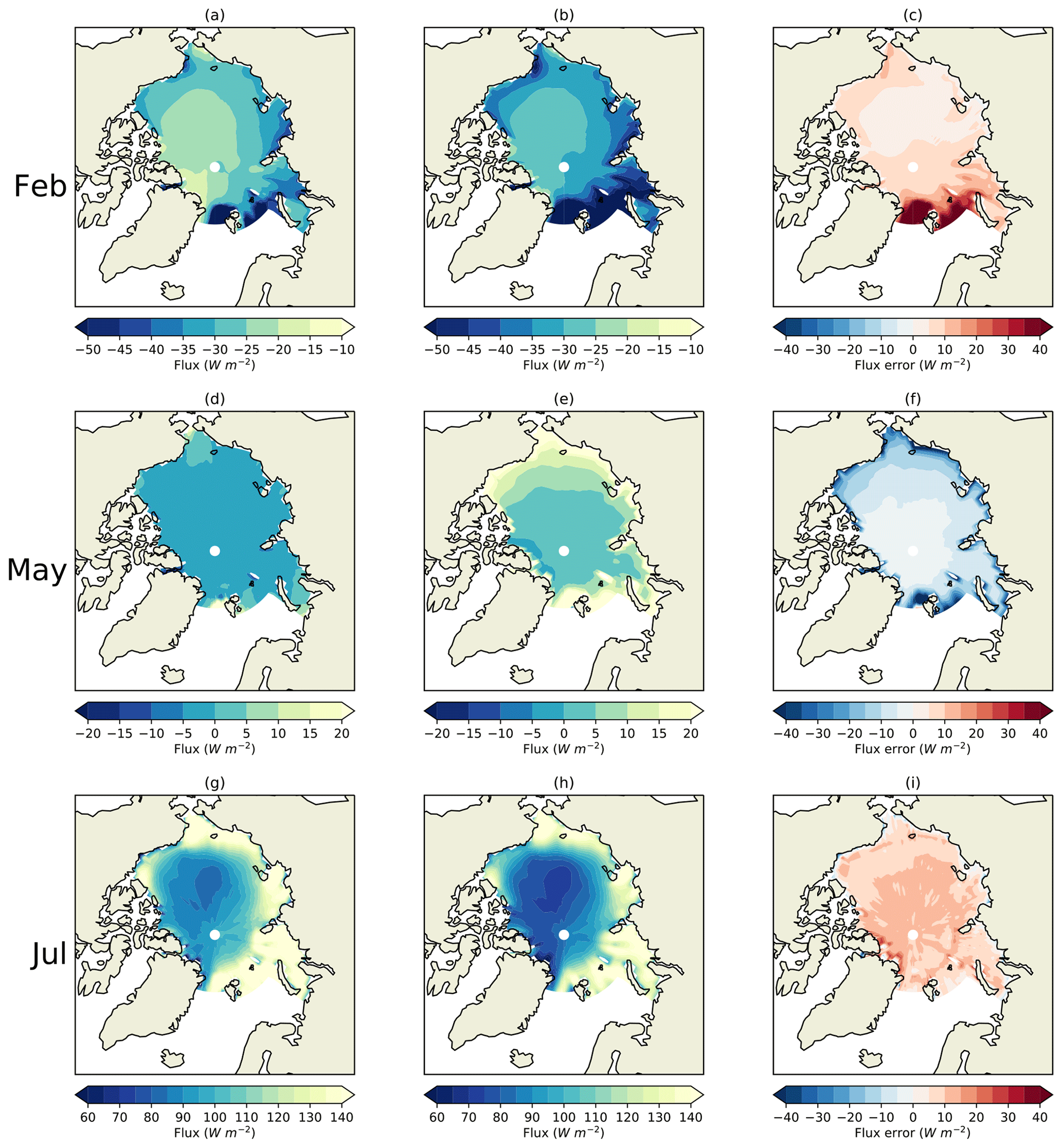
Figure B1Illustrating approximated (left) and actual (centre) model net surface flux, as well as the approximation error (right), in (a)–(c) February; (d)–(f) May; (g)–(i) July, for the period 1980–1999 in the first historical run of HadGEM2-ES.
More generally, the difference between the surface flux bias and the sum of the induced surface flux biases can be approximated by , a term that can be calculated relatively easily as many of the derivatives go to zero. Averaged over the Arctic Ocean, this term was small (below 1 Wm−2 in magnitude) in most months of the year but was of significant size in October (3.6 Wm−2) due to co-location of substantial negative biases in downwelling LW and category 1 ice thickness in this month, indicating that the true surface flux bias in this month may be substantially smaller (in absolute terms) than the −11.5 Wm−2 obtained from the summing of the ISF biases.
Finally, the induced surface flux calculation implicitly assumes a linear dependence of surface flux on each climate variable. However, this is not the case for the ice thickness, where higher-order derivatives do not go to zero and in some regions of thinner ice actually diverge. It is possible to quantify the error introduced by the assumption of linearity by comparing the partial derivative to the quantity , where , being climatological ice thickness in the reference dataset, in this case PIOMAS, and all other terms defined as in Sect. 4. It can be shown that multiplying this quantity by the model bias produces the exact bias in estimated surface flux that is being approximated by . Hence the bias in the ice thickness component induced by the nonlinearity can be calculated directly. It is found that the nonlinearity causes the ice thickness component to be overestimated in magnitude by 0.7 Wm−2 on average from October to April, with a maximum overestimation of 1.9 Wm−2 in November.
The code used to create the fields of induced surface flux bias is written in Python and is provided as a Supplement (directory “ISF”). The code used to create Figs. 1–9, as well as Fig. B1, is also provided (directory “Figures”). In addition, the routines used to estimate errors in the ISF analysis are provided (directory “Analysis”). Finally, the code used to create Table 1 is provided (directory “Tables”). A set of auxiliary routines used by most of the above are also provided (directory “Library”). Most routines make use of the open-source Iris library, and several make use of the open-source Cartopy library.
Monthly mean ice thickness, ice fraction, snow thickness and surface radiation, as well as daily surface temperature and surface radiation, for the historical simulations of HadGEM2-ES, are available from the CMIP5 archive at https://cmip.llnl.gov/cmip5/data_portal.html (last access: February 2018).
NSIDC ice concentration and melt onset data can be downloaded at http://nsidc.org/data/NSIDC-0051 (last access: May 2017; Cavalieri et al., 1996) and http://nsidc.org/data/NSIDC-0105 (last access: March 2016; Anderson et al., 2011) respectively.
PIOMAS ice thickness data can be downloaded at http://psc.apl.uw.edu/research/projects/arctic-sea-ice-volume-anomaly/data/ (last access: March 2016; Zhang and Rothrock, 2003).
ERAI surface radiation data can be downloaded at http://apps.ecmwf.int/datasets/data/interim-full-daily/levtype=sfc/ (last access: September 2016; Dee et al., 2011).
ISCCP-FD surface radiation data are available at https://isccp.giss.nasa.gov/projects/browse_fc.html (last access: October 2015; Zhang et al., 2004).
CERES surface radiation data are available at https://climatedataguide.ucar.edu/climate-data/ceres-ebaf. (last access: August 2014; Loeb et al., 2009)
The supplement related to this article is available online at: https://doi.org/10.5194/tc-13-2001-2019-supplement.
The induced surface flux framework was devised and carried out by AW. Model evaluation was also carried out by AW. MC and EB gave high-level advice concerning research direction, level of complexity and appropriate conclusions. Radiation reference datasets were chosen and evaluated, and winter radiation cloud biases interpreted, with advice from JR and ABS. EB, MC and JR gave much assistance in editing the manuscript at every stage.
The authors declare that they have no conflict of interest.
This work was supported by the Joint UK BEIS/Defra Met Office Hadley Centre Climate Programme (GA01101) and the European Union's Horizon 2020 Research & Innovation programme through grant agreement no. 727862 APPLICATE. MC was supported by NE/N018486/1.
The authors thank Francois Massonnet, Martin Vancoppenolle and the topical editor Dirk Notz for the thorough analysis, useful comments and suggestions made on multiple versions of this study. Thanks are also due to Richard Wood and Ann Keen for the helpful comments on multiple versions of this study.
This research has been supported by the Joint UK BEIS/Defra Met Office Hadley Centre Climate Programme (grant no. GA01101) and the European Union's Horizon 2020 Research & Innovation programme (grant no. 727862) APPLICATE. Mat Collins was supported by the Natural Environment Research Council, UK (grant no. NE/N018486/1).
This paper was edited by Dirk Notz and reviewed by Francois Massonnet and Martin Vancoppenolle.
Anderson, M., Bliss, A., and Drobot, S.: Snow Melt Onset Over Arctic Sea Ice from SMMR and SSM/I-SSMIS Brightness Temperatures, Version 3, Boulder, Colorado USA, NASA National Snow and Ice Data Center Distributed Active Archive Centerm https://doi.org/10.5067/22NFZL42RMUO, 2011 (updated 2012).
Bitz, C. M.: Some Aspects of Uncertainty in Predicting Sea Ice Thinning, in: Arctic Sea Ice Decline: Observations, Projections, Mechanisms, and Implications, edited by: DeWeaver, E. T., Bitz, C. M., and Tremblay, L.-B., American Geophysical Union, Washington, D.C., https://doi.org/10.1029/180GM06, 2008.
Bitz, C. M. and Roe, G. H.: A Mechanism for the High Rate of Sea Ice Thinning in the Arctic Ocean, J. Climate, 17, 3623–3632, https://doi.org/10.1175/1520-0442(2004)017<3623:AMFTHR>2.0.CO;2, 2004.
Bitz, C. M., Holland, M. M., Hunke, E. C., and Moritz, R. M.: Maintenance of the Sea-Ice Edge, J. Climate, 18, 2903–2921, https://doi.org/10.1175/JCLI3428.1, 2005.
Boeke, R. C. and Taylor, P. C.: Evaluation of the Arctic surface radiation budget in CMIP5 models, J. Geophys. Res.-Atmos., 121, 8525–8548, https://doi.org/10.1002/2016JD025099, 2016.
Cavalieri, D. J., Parkinson, C. L., Gloersen, P., and Zwally, H. J.: updated yearly. Sea Ice Concentrations from Nimbus-7 SMMR and DMSP SSM/I-SSMIS Passive Microwave Data, Version 1. (1980–1999), Boulder, Colorado USA, NASA National Snow and Ice Data Center Distributed Active Archive Center, https://doi.org/10.5067/8GQ8LZQVL0VL, 1996.
Christensen, M. W., Behrangi, A., L'ecuyer, T. S., Wood, N. B., Lebsock, M. D., and Stephens, G. L.: Arctic Observation and Reanalysis Integrated System: A New Data Product for Validation and Climate Study, B. Am. Meteorol. Soc., 97, 907–916, https://doi.org/10.1175/BAMS-D-14-00273.1, 2016.
Collins, W. J., Bellouin, N., Doutriaux-Boucher, M., Gedney, N., Halloran, P., Hinton, T., Hughes, J., Jones, D., Joshi, M., Liddicoat, S., Martin, G., O'Connor, F., Rae, J., Senior, C., Sitch, S., Totterdell, I., Wiltshire, A., and Woodward, S.: Development and evaluation of an Earth-System model – HadGEM2, Geosci. Model Dev., 4, 1051–1075, https://doi.org/10.5194/gmd-4-1051-2011, 2011.
Dee, D. P, Uppala, S. M., Simmons, A. J., Berrisford, P., Poli, P., Kobayashi, S., Andrae, U., Balmaseda, M. A., Balsamo, G., Bauer, P., Bechtold, P., Beljaars, A. C. M., van de Berg, L., Bidlot, J., Bormann, N., Belsol, C., Dragani, R., Fuentes, M., Geer, A., J., Haimberger, L., Healy, S. B., Hersbach, H., Holm, E. V., Isaksen, L., Kållberg, P., Köhler, M., Matricardi, M., McNally, A. P., Monge-Sanz, B. M., Morcrette, J.-J., Park, B.-K., Peubey, C., de Rosnay, P., Tavolato, C., Thépaut, J.-N., and Vitart, F.: The ERA-Interim reanalysis: configuration and performance of the data assimilation system, Q. J. Roy. Meteorol. Soc., 137, 553–597, https://doi.org/10.1002/qj.828, 2011.
DeWeaver, E. T., Hunke, E. C., and Holland, M. M.: Sensitivity of Arctic Sea Ice Thickness to Intermodel Variations in the Surface Energy Budget. AGU Geophysical Monograph 180: Arctic Sea Ice Decline: Observations, Projections, Mechan. Imp., 180, 77–91, https://doi.org/10.1029/180GM07, 2008.
HadGEM2 Development Team: G. M. Martin, Bellouin, N., Collins, W. J., Culverwell, I. D., Halloran, P. R., Hardiman, S. C., Hinton, T. J., Jones, C. D., McDonald, R. E., McLaren, A. J., O'Connor, F. M., Roberts, M. J., Rodriguez, J. M., Woodward, S., Best, M. J., Brooks, M. E., Brown, A. R., Butchart, N., Dearden, C., Derbyshire, S. H., Dharssi, I., Doutriaux-Boucher, M., Edwards, J. M., Falloon, P. D., Gedney, N., Gray, L. J., Hewitt, H. T., Hobson, M., Huddleston, M. R., Hughes, J., Ineson, S., Ingram, W. J., James, P. M., Johns, T. C., Johnson, C. E., Jones, A., Jones, C. P., Joshi, M. M., Keen, A. B., Liddicoat, S., Lock, A. P., Maidens, A. V., Manners, J. C., Milton, S. F., Rae, J. G. L., Ridley, J. K., Sellar, A., Senior, C. A., Totterdell, I. J., Verhoef, A., Vidale, P. L., and Wiltshire, A.: The HadGEM2 family of Met Office Unified Model climate configurations, Geosci. Model Dev., 4, 723–757, https://doi.org/10.5194/gmd-4-723-2011, 2011.
Holland, M. M., Serreze, M. C., and Stroeve, J.: The sea ice mass budget of the Arctic and its future change as simulated by coupled climate models, Clim. Dynam., 34, 185–200, https://doi.org/10.1007/s00382-008-0493-4, 2010.
Hunke, E. C. and Dukowicz, J. K.: An Elastic-Viscous-Plastic Model for Sea Ice Dynamics, J. Phys. Oceanogr., 27, 1849–1867, https://doi.org/10.1175/1520-0485(1997)027<1849:AEVPMF>2.0.CO;2, 1997.
Johns, T. C., Durman, C. F., Banks, H. T., Roberts, M. J., McLaren, A. J., Ridley, J. K., Senior, C. A., Williams, K. D., Jones, A., Rickard, G. J., Cusack, S., Ingram, W. J., Crucifix, M., Sexton, D. M. H., Joshi, M. M., Dong, B.-W., Spencer, H., Hill, R. S. R., Gregory, J. M., Keen, A. B., Pardaens, A. K., Lowe, J. A., Bodas-Salcedo, A., Stark, S., and Searl, Y.: The New Hadley Centre Climate Model (HadGEM1): Evaluation of Coupled Simulations, J. Climate, 19, 1327–1353, https://doi.org/10.1175/JCLI3712.1, 2006.
Keen, A. and Blockley, E.: Investigating future changes in the volume budget of the Arctic sea ice in a coupled climate model, The Cryosphere, 12, 2855–2868, https://doi.org/10.5194/tc-12-2855-2018, 2018.
Laxon, S., Peacock, N., and Smith, D.: High interannual variability of sea ice thickness in the Arctic region, Nature, 425, 947–950, https://doi.org/10.1038/nature02050, 2003.
Laxon, S., Giles, K. A., Ridout, A., Wingham, D. J., Willatt, R., Cullen, R., Kwok, R., Schweiger, A., Zhang, J., Haas, C., Hendricks, S., Krishfield, R., Kurtz, N., Farrell, S., and Davidson, M.: Cryosat-2 estimates of Arctic sea ice thickness and volume, Geophys. Res. Lett., 40, 732–737, https://doi.org/10.1002/grl.50193, 2013.
Lindsay, R.: Temporal Variability of the Energy Balance of Thick Arctic Pack Ice, J. Climate, 11, 313–333, https://doi.org/10.1175/1520-0442(1998)011<0313:TVOTEB>2.0.CO;2, 1998.
Lindsay, R., Wensnahan, M., Schweiger, A., and Zhang, J.: Evaluation of Seven Difference Atmospheric Reanalysis Products in the Arctic, J. Climate, 27, 2588–2606, https://doi.org/10.1175/JCLI-D-13-00014.1, 2014.
Lindsay, R. and Schweiger, A.: Arctic sea ice thickness loss determined using subsurface, aircraft, and satellite observations, The Cryosphere, 9, 269–283, https://doi.org/10.5194/tc-9-269-2015, 2015.
Lipscomb, W. H. and Hunke, E. C., Modeling Sea Ice Transport Using Incremental Remapping, Mon. Weather Rev., 132, 1341–1354, https://doi.org/10.1175/1520-0493(2004)132<1341:MSITUI>2.0.CO;2, 2004.
Liu, J., Curry, J. A., Rossow, W. B., Key, J. R., and Wang, X.: Comparison of surface radiative flux data sets over the Arctic Ocean, J. Geophys. Res.-Oceans, 110, C02015, https://doi.org/10.1029/2004JC002381, 2005.
Loeb, N. G., Wielicki, B. A., Doelling, D. R., Louis Smith, G., Keyes, D. F., Kato, S., Manalo-Smith, N., and Wong, T.: Toward Optimal Closure of the Earth's Top-of-Atmosphere Radiation Budget, J. Climate, 22, 748–766, https://doi.org/10.1175/2008JCLI2637.1, 2009.
Markus, T., Stroeve, J. C., and Miller, J.: Recent changes in Arctic sea ice melt onset, freezeup, and melt season length, J. Geophys. Res., 114, C12024, https://doi.org/10.1029/2009JC005436, 2009.
Maslanik, J., Stroeve, J. C., Fowler, C., and Emery, W.: Distribution and trends in Arctic sea ice age through spring 2011, Geophys. Res. Lett., 38, 47735, https://doi.org/10.1029/2011GL047735, 2011.
Massonnet, F., Fichefet, T., Goosse, H., Bitz, C. M., Philippon-Berthier, G., Holland, M. M., and Barriat, P.-Y.: Constraining projections of summer Arctic sea ice, The Cryosphere, 6, 1383–1394, https://doi.org/10.5194/tc-6-1383-2012, 2012.
Massonnet, F., Vancoppenolle, M., Goosse, H., Docquier, D., Fichefet, T., and Blanchard-Wrigglesworth, E., Arctic sea-ice change tied to its mean state through thermodynamic processes, Nat. Clim. Ch., 8, 599–603, https://doi.org/10.1038/s41558-018-0204-z, 2018.
Maykut, G. A. and McPhee, M. G., Solar heating of the Arctic mixed layer, J. Geophys. Res., 100, 24691–24703, https://doi.org/10.1029/95JC02554, 1995.
McLaren, A. J., Banks, H. T., Durman, C. F., Gregory, J. M., Johns, T. C., Keen, A. B., Ridley, J. K., Roberts, M. J., Lipscomb, W. H., Connolley, W. M., and Laxon, S. W.: Evaluation of the sea ice simulation in a new coupled atmosphere-ocean climate model (HadGEM1), J. Geophys. Res., 111, C12014, https://doi.org/10.1029/2005JC003033, 2006.
McPhee, M. G., Kikuchi, T., Morison, J. H., and Stanton, T. P.: Ocean-to-ice heat flux at the North Pole environmental observatory, Geophys. Res. Lett., 30, 2274, https://doi.org/10.1029/2003GL018580, 2003.
Notz, D.: How well must climate models agree with observations?, Philos. T. Roy. Soc. A, 373, 20140164, https://doi.org/10.1098/rsta.2014.0164, 2015.
Perovich, D. K. and Elder, B., Estimates of ocean heat flux at SHEBA, Geophys. Res. Lett., 299, 58-1–51-4, https://doi.org/10.1029/2001GL014171, 2002.
Perovich, D. K., Richter-Menge, J. A., Jones, K. F., and Light, B.: Sunlight, water, and ice: Extreme Arctic sea ice melt during the summer of 2007, Geophys. Res. Lett., 35, L11501, https://doi.org/10.1029/2008GL034007, 2008.
Pithan, F., Medeiros, B., and Mauritsen, T.: Mixed-phase clouds cause climate model biases in Arctic wintertime temperature inversions, Clim. Dynam., 43, 289–303, https://doi.org/10.1007/s00382-013-1964-9, 2014.
Raddatz, R. L., Papakyriakou, T. N., Else, B. G., Asplin, M. G., Candlish, L. M., Galley, R. J., and Barber, D. G.: Downwelling longwave radiation and atmospheric winter states in the western maritime Arctic, Int. J. Clim., 35, 2339–2351, https://doi.org/10.1002/joc.4149, 2014.
Rayner, N. A., Parker, D. E., Horton, E. B., Folland, C. K., Alexander, L. V., Rowell, D. P., Kent, E. C., and Kaplan, A.: Global analyses of sea surface temperature, sea ice, and night marine air temperature since the late nineteenth century, J. Geophys. Res., 108, 4407, https://doi.org/10.1029/2002JD002670, 2003.
Rothrock, D. A., Percival., D. B., and Wensnahan, M.: The decline in arctic sea ice thickness: Separating the spatial., annual., and interannual variability in a quarter century of submarine data, J. Geophys. Res., 113, C05003, https://doi.org/10.1029/2007JC004252, 2008.
Rutan, D. A., Kato, S., Doelling, D. R., Rose, F. G., Nguyen, L. T., Caldwell, T. E., and Loeb, N. G.: CERES Synoptic Product: Methodology and Validation of Surface Radiant Flux, J. Atmos. Ocean. Technol., 32, 1121–1143, https://doi.org/10.1175/JTECH-D-14-00165.1, 2015.
Schauer, U., Fahrbach, E., Osterhus, S., and Rohardt,, G.: Arctic warming through Fram Strait: Oceanic heat transport from 3 years of measurements, J. Geophys. Res.-Oceans, 109, C06026, https://doi.org/10.1029/2003JC001823, 2004.
Semtner, A. J.: A Model for the Thermodynamic Growth of Sea Ice in Numerical Investigations of Climate, J. Phys. Oceanogr., 6, 379–389, https://doi.org/10.1175/1520-0485(1976)006<0379:AMFTTG>2.0.CO;2, 1976.
Serreze, M. C., Barrett, A. P., Slater, A. G., Woodgate, R. A., Aagaard, K., Lammers, R. B., Steele. M., Moritz, R., Meredith, M., and Lee, C. M.: The large-scale freshwater cycle of the Arctic, J. Geophys. Res., 111, C11010, https://doi.org/10.1029/2005JC003424, 2006.
Serreze, M. C., Barratt, A. P., Slater, A. G., Steele, M., Zhang, J., and Trenberth, K. E.: The large-scale energy budget of the Arctic, J. Geophys. Res., 112, D11122, https://doi.org/10.1029/2006JD008230, 2007.
Shu, Q., Song, Z., and Qiao, F.: Assessment of sea ice simulations in the CMIP5 models, The Cryosphere, 9, 399–409, https://doi.org/10.5194/tc-9-399-2015, 2015.
Stammerjohn, S., Massom, R., Rind, D., and Martinson, D: Regions of rapid sea ice change: An inter-hemispheric seasonal comparison, Geophys. Res. Lett., 39, L06501, https://doi.org/10.1029/2012GL050874, 2012.
Steele, M., Zhang, J., and Ermold, W.: Mechanisms of summer Arctic Ocean warming, J. Geophys. Res.-Oceans, 115, C11004, https://doi.org/10.1029/2009JC005849, 2010.
Stramler, K., Del Genio, A. D., and Rossow, W. B.: Synoptically Driven Arctic Winter States, J. Climate, 24, 1747–1762, https://doi.org/10.1175/2010JCLI3817.1, 2011.
Stroeve, J. C., Kattsov, V, Barrett, A., Serreze, M., Pavlova, T., Holland, M. M., and Meier, W. N.: Trends in Arctic sea ice extent from CMIP5, CMIP3 and observations, Geophys. Res. Lett., 39, L16502, https://doi.org/10.1029/2012GL052676, 2012a.
Stroeve, J. C., Serreze, M. C., Holland, M. M., Kay, J. E., Maslanik, J., and Barratt, A. P.: The Arctic's rapidly shrinking sea ice cover: a research synthesis, Clim. Ch., 110, 1005–1027, https://doi.org/10.1007/s10584-011-0101-1, 2012b.
Swart, N. C., Fyfe, J. C., Hawkins, E., Kay, J. E., and Jahn, A.: Influence of internal variability on Arctic sea ice trends, Nat. Clim. Ch., 5, 86–89, https://doi.org/10.1038/nclimate2483, 2015.
Thorndike, A. S., Rothrock, D. A., Maykut, G. A., and Colony, R., The thickness distribution of sea ice, J. Geophys. Res., 80, 4501–4513, https://doi.org/10.1029/JC080i033p04501, 1975.
Titchner, H. A. and Rayner, N. A.: The Met Office Hadley Centre sea ice and sea surface temperature data set, version 2: 1. Sea ice concentrations, J. Geophys. Res.-Atmos., 119, 2864–2889, https://doi.org/10.1002/2013JD020316, 2014.
Tsamados, M., Feltham, D. L., and Wilchinsky, A. V., Impact of a new anisotropic rheology on simulations of Arctic sea ice, J. Geophys. Res.-Oceans, 118, 91–107, https://doi.org/10.1029/2012JC007990, 2013.
Wang, M. and Overland, J. E.: A sea ice free summer Arctic within 30 years: An update from CMIP5 models. Geophys. Res. Lett., 39, L18501, https://doi.org/10.1029/2012GL052868, 2012.
Wang, X., Key, J., Kwok, R., and Zhang, J.: Comparison of Arctic Sea Ice Thickness from Satellites, Aircraft and PIOMAS data, Remote Sens., 8, 713, https://doi.org/10.3390/rs8090713, 2016.
Zhang, J. and Rothrock, D. A.: Modeling Global Sea Ice with a Thickness and Enthalpy Distribution Model in Generalized Curvilinear Coordinates, Mon. Weather Rev., 131, 845–861, https://doi.org/10.1175/1520-0493(2003)131<0845:MGSIWA>2.0.CO;2, 2003
Zhang, Y., Rossow, W. B., Lacis, A. A., Oinas, V., and Mishchenko, M. I.: Calculation of radiative fluxes from the surface to top of atmosphere based on ISCCP and other global data sets: Refinements of the radiative transfer model and the input data, J. Geophys. Res., 109, D19105, https://doi.org/10.1029/2003JD004457, 2004.
- Abstract
- Copyright statement
- Introduction
- Model and reference datasets
- Evaluating HadGEM2-ES
- The induced surface flux (ISF) framework: a way to quantify the effect of each model bias on sea ice volume balance
- Induced surface flux biases
- Discussion
- Conclusions
- Appendix A: Description and derivation of the surface flux formula used in the ISF calculation
- Appendix B: Analysis of potential errors in ISF bias calculation
- Code availability
- Data availability
- Author contributions
- Competing interests
- Acknowledgements
- Financial support
- Review statement
- References
- Supplement