Sensitivity of centennial mass loss projections of the Amundsen basin to the friction law

Reliable projections of ice sheets' future contributions to sea-level rise require models that are able to accurately simulate grounding-line dynamics, starting from initial states consistent with observations. Here, we simulate the centennial evolution of the Amundsen Sea Embayment in response to a prescribed perturbation in order to assess the sensitivity of mass loss projections to the chosen friction law, depending on the initialisation strategy. To this end, three different model states are constructed by inferring both the initial basal shear stress and viscosity fields with various relative weights. Then, starting from each of these model states, prognostic simulations are carried out using a Weertman, a Schoof and a Budd friction law, with different parameter values. Although the sensitivity of projections to the chosen friction law tends to decrease when more weight is put on viscosity during initialisation, it remains significant for the most physically acceptable of the constructed model states. Independently of the considered model state, the Weertman law systematically predicts the lowest mass losses. In addition, because of its particular dependence on effective pressure, the Budd friction law induces significantly different grounding-line retreat patterns than the other laws and predicts significantly higher mass losses.

1 Introduction

The West Antarctic Ice Sheet mean annual contribution to global sea-level rise (SLR) has tripled over the last 25 years as a consequence of a growing imbalance between the mass it receives as snowfall and that which is discharged to the ocean by ice streams (Shepherd et al., 2018). The most active basin of this region is the Amundsen Sea Embayment (ASE), where marine-terminating outlet glaciers draining ice to the oceans have shown sustained acceleration and thinning over the last decades, with their grounding lines (GLs), i.e. the limit between the grounded ice sheet and the floating ice shelf, retreating at rates higher than 1 km a⁻¹ since 1992 (Mouginot et al., 2014; Rignot et al., 2014). These observations raise concerns regarding the near future of the ASE as they suggest that this sector of West Antarctica is undergoing a marine ice-sheet instability (MISI), which would imply a significant additional global SLR in the coming decades (Cornford et al., 2015; Favier et al., 2014; Joughin et al., 2014). Producing reliable estimates of this future contribution requires accurate modelling of GL dynamics on sub-centennial timescales as well as the ability to produce model states that are as close as possible to observations.

Using a synthetic flow line geometry, Brondex et al. (2017) have shown that the GL dynamics depends critically on the choice of the friction law, i.e. the mathematical relationship linking basal shear stress to other parameters including sliding velocity. The ice–bed interface being usually out of reach, the formulation of a friction law has been a long-standing problem in glaciology. Various laws intended to describe different physical processes at the roots of basal motion have been developed over the years (Budd et al., 1979; Schoof, 2005; Tsai et al., 2015; Weertman, 1957). Most ice flow modelling studies published so far use the Weertman friction law, which aims to describe the basal motion of ice over and around obstacles of a rigid bedrock by a combination of viscous creep and regelation (Weertman, 1957). However, many rapid ice streams of Antarctica are known to be lying on soft beds made of water-laden till, the deformation of which explains most of the motion observed at the surface (Alley et al., 1986; Blankenship et al., 1986; Kavanaugh and Clarke, 2006). Numerous laboratory studies on till samples and in situ measurements have shown that, at large strain, the till rheology is plastic with a critical strength τ^* depending on effective pressure N, i.e. the difference between ice overburden pressure and water pressure (Alley et al., 1986; Blankenship et al., 1986; Boulton and Jones, 1979). To account for both the cases of rigid and soft beds, Tsai et al. (2015) proposed a law inducing a Coulomb friction regime at low N, which instantaneously switches to a Weertman friction regime at higher N. By construction, this law induces an upper-bound function of N of the basal shear stress. Although it was originally intended to describe the ice flowing over a rigid bed with the opening of water-filled cavities, the law proposed by Schoof (2005) behaves similarly, except that the transition between the Coulomb and Weertman regimes is continuous, which makes it easier to handle numerically (Brondex et al., 2017).

Although a growing amount of information about the current state of the ice-sheet (e.g. surface velocities, surface elevation, surface elevation rates of change) is made available by the rapid development of satellite observations, several model parameters remain poorly constrained (e.g. bedrock elevation, ice viscosity, friction law coefficients). Gradient-based optimisation methods are routinely used to estimate uncertain model parameter fields and boundary conditions so that the initial ice-sheet geometry and surface velocity field are as close as possible to the observations (Cornford et al., 2015; Gillet-Chaulet et al., 2012; Morlighem et al., 2010, 2013). Although such methods enable us to deduce the current basal shear stress field from observed surface velocities, the form of the friction law cannot be discriminated with a unique set of observations (Gillet-Chaulet et al., 2016; Joughin et al., 2004). Furthermore, when several uncertain fields are simultaneously inferred, several different initial states consistent with observations can potentially be constructed. Adhalgeirsdóttir et al. (2014) have shown that SLR projections on decadal timescales are sensitive to the initial state of the model, which can account for an important source of uncertainty in the model response.

In the present study, we aim to assess the relative sensitivity of centennial mass loss projections of the ASE to the chosen friction law and initialisation strategy. Our work being based on a prescribed perturbation scenario, the results presented here should not be considered as actual projections of the future contribution of the ASE to SLR. The first step consists of building three different model states of the ASE by simultaneously inferring the basal shear stress and the ice viscosity, with various relative weights attributed to each one of these two fields during the inversion. Then, for each of these states, we follow the same procedure as in Brondex et al. (2017) to identify the distributions of the friction coefficients of three commonly used friction laws that lead to the same model initial states. Finally, we apply a synthetic perturbation to the basal melting rate under floating ice, to the different initial states and compare the dynamical responses obtained with the various friction laws. In Sect. 2, we give a precise description of the model used to conduct this study and describe the experimental setup. The results obtained at each step of the experiments are presented in Sect. 3 and discussed in the last section.

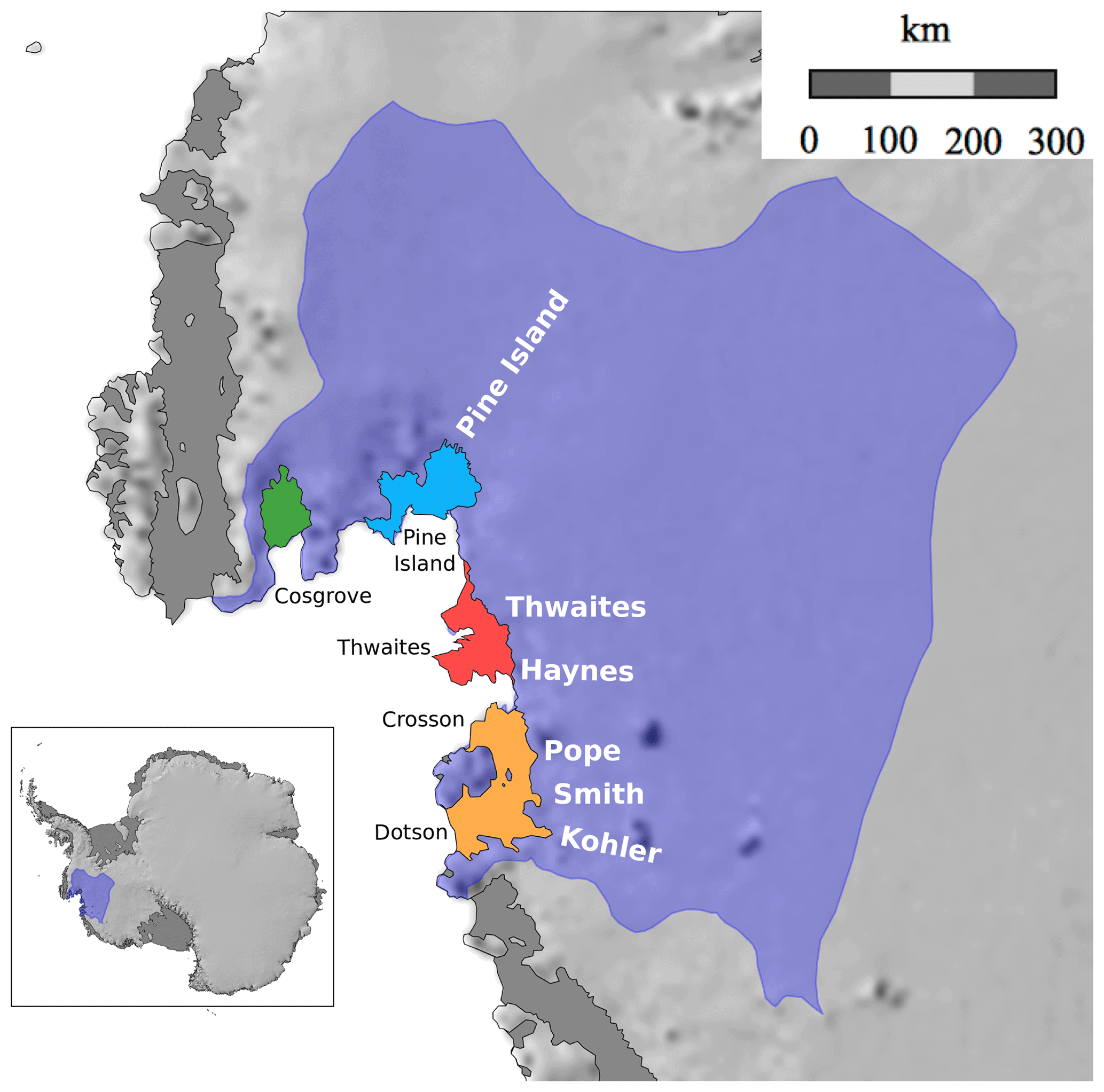
Figure 1 Amundsen Sea Embayment (ASE) and its ice shelves: Cosgrove (green), Pine Island (blue, fed by the Pine Island Glacier), Thwaites (red, fed by the Thwaites and Haynes ice streams), Crosson and Dotson (yellow, fed by the Pope, Smith and Kohler ice streams). The localisation of the ASE is reported on the map of Antarctica in the bottom-left corner (purple).

2 Methods

2.1 Model description

The modelled domain is represented in Fig. 1. For the stress balance, we solve the two-dimensional Shelfy-Stream Approximation (SSA) equations (MacAyeal, 1989), for which the horizontal velocity field $\mathbf{u}=(u,v)$ is a solution of

$$\begin{array}{ll}{\displaystyle }\mathrm{4}{\displaystyle \frac{\partial }{\partial x}}\left(H\stackrel{\mathrm{‾}}{\mathit{\eta }}{\displaystyle \frac{\partial u}{\partial x}}\right)+\mathrm{2}{\displaystyle \frac{\partial }{\partial x}}\left(H\stackrel{\mathrm{‾}}{\mathit{\eta }}{\displaystyle \frac{\partial v}{\partial y}}\right)& {\displaystyle }+{\displaystyle \frac{\partial }{\partial y}}\left(H\stackrel{\mathrm{‾}}{\mathit{\eta }}\left({\displaystyle \frac{\partial u}{\partial y}}+{\displaystyle \frac{\partial v}{\partial x}}\right)\right)\\ {\displaystyle }& {\displaystyle }+{\mathit{\tau }}_{\text{b},x}={\mathit{\rho }}_{\text{i}}gH{\displaystyle \frac{\partial z_{\text{s}}}{\partial x}}\end{array}$$

$$\begin{array}{ll}{\displaystyle }\mathrm{4}{\displaystyle \frac{\partial }{\partial y}}\left(H\stackrel{\mathrm{‾}}{\mathit{\eta }}{\displaystyle \frac{\partial v}{\partial y}}\right)+\mathrm{2}{\displaystyle \frac{\partial }{\partial y}}\left(H\stackrel{\mathrm{‾}}{\mathit{\eta }}{\displaystyle \frac{\partial u}{\partial x}}\right)& {\displaystyle }+{\displaystyle \frac{\partial }{\partial x}}\left(H\stackrel{\mathrm{‾}}{\mathit{\eta }}\left({\displaystyle \frac{\partial u}{\partial y}}+{\displaystyle \frac{\partial v}{\partial x}}\right)\right)\\ \text{(1)}& {\displaystyle }& {\displaystyle }+{\mathit{\tau }}_{\text{b},y}={\mathit{\rho }}_{\text{i}}gH{\displaystyle \frac{\partial z_{\text{s}}}{\partial y}},\end{array}$$

where ρ_i is the ice density, g is the gravity norm and $H=z_{\text{s}}-z_{\text{b}}$ is the ice thickness, with z_s and z_b the top and bottom surface elevations. The vertically averaged effective viscosity $\stackrel{\mathrm{‾}}{\mathit{\eta }}$ reads as follows:

$$\begin{array}{}\text{(2)}& \stackrel{\mathrm{‾}}{\mathit{\eta }}={\stackrel{\mathrm{‾}}{\mathit{\eta }}}_{\mathrm{0}}{D}_e^{(\mathrm{1}-n)/n},\end{array}$$

where D_e is the second invariant of the strain-rate tensor, n is the Glen's law exponent and ${\stackrel{\mathrm{‾}}{\mathit{\eta }}}_{\mathrm{0}}$ is given by

$$\begin{array}{}\text{(3)}& {\stackrel{\mathrm{‾}}{\mathit{\eta }}}_{\mathrm{0}}={\displaystyle \frac{\mathrm{1}}{H}}\underset{z_{\text{b}}}{\overset{z_{\text{s}}}{\int }}{\displaystyle \frac{\mathrm{1}}{\mathrm{2}}}{A}^{-\mathrm{1}/n}\text{d}z.\end{array}$$

In Eq. (3), A is the rate factor. It is related to the temperature relative to the pressure-melting point T^′ (^∘C) through an Arrhenius law:

$$\begin{array}{}\text{(4)}& A=A_{\mathrm{0}}{e}^{\left(-Q/\left[R\right(\mathrm{273.15}+T^{\prime }]\right)},\end{array}$$

where A₀ is the pre-exponential factor, Q is an activation energy and R is the gas constant (Cuffey and Paterson, 2010).

For the basal shear stress τ_b in Eq. (), we consider three different friction laws:

$$\begin{array}{}\text{(5)}& {\displaystyle }& {\displaystyle }{\mathit{\tau }}_{\text{b}}+C_{\text{W}}|{\mathbf{u}}_{\text{b}}{|}^{m-\mathrm{1}}{\mathbf{u}}_{\text{b}}=\mathrm{0},\text{(6)}& {\displaystyle }& {\displaystyle }{\mathit{\tau }}_{\text{b}}+C_{\text{B}}N|{\mathbf{u}}_{\text{b}}{|}^{m-\mathrm{1}}{\mathbf{u}}_{\text{b}}=\mathrm{0},\text{(7)}& {\displaystyle }& {\displaystyle }{\mathit{\tau }}_{\text{b}}+{\displaystyle \frac{C_{\text{S}}|{\mathbf{u}}_{\text{b}}{|}^{m-\mathrm{1}}{\mathbf{u}}_{\text{b}}}{{\left(\mathrm{1}+{\left(\frac{C_{\text{S}}}{C_{\text{max}}N}\right)}^{\mathrm{1}/m}\left|{\mathbf{u}}_{\text{b}}\right|\right)}^m}}=\mathrm{0},\end{array}$$

where C_W, C_B and C_S are friction parameters. Equation (5) corresponds to the widely used Weertman law (Weertman, 1957), where m is a positive exponent, often related to the creep exponent n of the Glen's law as $m=\mathrm{1}/n$. Equations (6) and (7) correspond to the Budd and Schoof friction laws, respectively (Budd et al., 1979; Schoof, 2005). Note that, on the contrary to the two other laws, the Schoof law induces an upper bound of the ratio $\left|{\mathit{\tau }}_{\text{b}}\right|/N$ known as Iken's bound that is equal to the value of the parameter C_max (Gagliardini et al., 2007; Iken, 1981; Schoof, 2005). Although it is not its original purpose, the use of a Schoof law – which can be seen as the equivalent of the Tsai law (Brondex et al., 2017) – is more and more justified by its ability to represent the deformation of till, as it induces a Coulomb friction regime at low N. In that case, the parameter C_max ought to be seen as a Coulomb friction parameter related to the rheological properties of the till. Laboratory measurements have shown that the values of C_max should then range between 0.17 and 0.84 (Cuffey and Paterson, 2010).

Both the Budd and Schoof laws make explicit use of the effective pressure N. Using an effective pressure-dependent friction law when running transient simulations proves necessary in order to account for the enhancement of basal sliding due to the presence of subglacial drainage systems connected to the ocean, which have been reported in several studies (Fricker et al., 2007; Gray et al., 2005; Le Brocq et al., 2013). However, unlike the Schoof law, for which the dependence of $\left|{\mathit{\tau }}_{\text{b}}\right|$ on N is limited to the close vicinity of the GLs, the Budd law induces a dependence of $\left|{\mathit{\tau }}_{\text{b}}\right|$ on N over the whole grounded part of the domain, even far into its interior where such a drainage system may not exist. Ideally, N should be computed by a subglacial hydrology model but the few available models of that kind usually rely on a multitude of poorly constrained parameters (Hewitt et al., 2012; Schoof, 2010; Werder et al., 2013; de Fleurian et al., 2014) and the attempts to couple these models to ice flow models are relatively recent (Bougamont et al., 2014; Bueler and van Pelt, 2015; Gagliardini and Werder, 2018; Hewitt, 2013). Therefore, in the present study, N is calculated assuming a perfect hydrological connection between the subglacial drainage system and the ocean, so that

$$\begin{array}{}\text{(8)}& N=\left\{\begin{array}{ll}{\mathit{\rho }}_{\text{i}}gH+{\mathit{\rho }}_{\text{w}}g{z}_{\text{b}}& \text{if}{z}_{\text{b}}<\mathrm{0},\\ {\mathit{\rho }}_{\text{i}}gH& \text{if}{z}_{\text{b}}\ge \mathrm{0},\end{array}\right.\end{array}$$

where ρ_w is the water density. A systematic comparison of the dependence of τ_b on N and u_b implied by these various friction laws is available in Brondex et al. (2017). Note that, since floating ice does not experience any friction, τ_b is set to zero wherever ice is afloat, independently of the chosen friction law.

The temporal evolution of ice thickness is governed by a two-dimensional mass transport equation:

$$\begin{array}{}\text{(9)}& {\displaystyle \frac{\partial H}{\partial t}}+{\displaystyle \frac{\partial \left(uH\right)}{\partial x}}+{\displaystyle \frac{\partial \left(vH\right)}{\partial y}}=a_{\text{s}}-a_{\text{b}},\end{array}$$

where a_s is the surface mass balance and a_b the oceanic melt rate applied to the bottom surface of the ice shelves only, basal melt at the ice–bed interface being neglected. Ice is assumed to be in hydrostatic equilibrium and the bottom surface elevation can be deduced from the bedrock topography b(x,y) by applying the no-penetration condition and the floating condition. Here we assume a constant sea level, z_sl=0, so that

$$\begin{array}{}\text{(10)}& \left\{\begin{array}{ll}{z}_{\text{b}}(x,y,t)=b(x,y)& \text{for grounded ice,}\\ z_{\text{b}}(x,y,t)=-H{\displaystyle \frac{{\mathit{\rho }}_{\text{i}}}{{\mathit{\rho }}_{\text{w}}}}>b(x,y)& \text{for floating ice}.\end{array}\right.\end{array}$$

The GL being the limit beyond which grounded ice starts floating, its position (x_G,y_G) can directly be deduced from Eq. (10) by solving the following:

$$\begin{array}{}\text{(11)}& H(x_{\text{G}},y_{\text{G}})+b(x_{\text{G}},y_{\text{G}}){\displaystyle \frac{{\mathit{\rho }}_{\text{w}}}{{\mathit{\rho }}_{\text{i}}}}=\mathrm{0}.\end{array}$$

Therefore, the GL can be located at any point of the domain and its position is free to evolve over time as a result of the evolving geometry.

The positions of the boundaries of the model domain are set based on the observations made by the satellite ICESat for the IMBIE2 effort (Zwally et al., 2012). In the following, $\mathbf{n}=(n_x,n_y)$ is the normal unit vector to the considered boundary. At the ice divides, there is no ice flux entering the domain, so the following Dirichlet condition applies:

$$\begin{array}{}\text{(12)}& (\mathbf{u}.\mathbf{n}){|}_{\text{id}}=\mathrm{0},\end{array}$$

and is completed by a free slip condition in the tangential direction. At the ice shelves and glaciers fronts, which remain fixed in time, the following Neumann condition applies:

$$\begin{array}{ll}{\displaystyle }\mathrm{4}H\stackrel{\mathrm{‾}}{\mathit{\eta }}{\left.{\displaystyle \frac{\partial u}{\partial x}}\right|}_{\text{f}}{n}_x& {\displaystyle }+\mathrm{2}H\stackrel{\mathrm{‾}}{\mathit{\eta }}{\left.{\displaystyle \frac{\partial v}{\partial y}}\right|}_{\text{f}}{n}_x+H\stackrel{\mathrm{‾}}{\mathit{\eta }}{\left.\left({\displaystyle \frac{\partial u}{\partial y}}+{\displaystyle \frac{\partial v}{\partial x}}\right)\right|}_{\text{f}}{n}_y\\ {\displaystyle }& {\displaystyle }={\displaystyle \frac{g}{\mathrm{2}}}({\mathit{\rho }}_{\text{i}}H{|}_{\text{f}}^{\mathrm{2}}-{\mathit{\rho }}_{\text{w}}{H}_{\text{sub}}{|}_{\text{f}}^{\mathrm{2}})n_x\\ {\displaystyle }\mathrm{2}H\stackrel{\mathrm{‾}}{\mathit{\eta }}{\left.{\displaystyle \frac{\partial u}{\partial x}}\right|}_{\text{f}}{n}_y& {\displaystyle }+\mathrm{4}H\stackrel{\mathrm{‾}}{\mathit{\eta }}{\left.{\displaystyle \frac{\partial v}{\partial y}}\right|}_{\text{f}}{n}_y+H\stackrel{\mathrm{‾}}{\mathit{\eta }}{\left.\left({\displaystyle \frac{\partial u}{\partial y}}+{\displaystyle \frac{\partial v}{\partial x}}\right)\right|}_{\text{f}}{n}_x\\ \text{(13)}& {\displaystyle }& {\displaystyle }={\displaystyle \frac{g}{\mathrm{2}}}({\mathit{\rho }}_{\text{i}}H{|}_{\text{f}}^{\mathrm{2}}-{\mathit{\rho }}_{\text{w}}{H}_{\text{sub}}{|}_{\text{f}}^{\mathrm{2}})n_y,\end{array}$$

where H_sub|_f is the submerged height at the considered front, which is null in the very few places where glacier fronts are grounded and relates to H|_f through the floating condition at floating fronts.

Similarly to Pollard and DeConto (2012), the oceanic melt rate a_b (m a⁻¹), prescribed on the bottom surface of ice shelves, is parameterised as follows:

$$\begin{array}{}\text{(14)}& a_{\text{b}}={\displaystyle \frac{\mathrm{8}{K}_{\text{T}}{\mathit{\rho }}_{\text{w}}{C}_{\text{W}}}{{\mathit{\rho }}_{\text{i}}{L}_{\text{f}}}}|T_{\mathrm{0}}-T_{\text{f}}|(T_{\mathrm{0}}-T_{\text{f}}),\end{array}$$

where T₀ and T_f are the ocean water temperature and freezing point at the considered depth, K_T is a transfer coefficient for sub-ice oceanic melting, C_W the specific heat of ocean water and L_f the latent heat of fusion of ice. Following Pollard and DeConto (2012), the temperature difference T₀−T_f is given by $T_{\mathrm{0}}-T_{\text{f}}=\mathrm{0.5}$ ^∘C for $\mathrm{0}>z>-\mathrm{170}$ m, 3.5 ^∘C for $z<-\mathrm{680}$ m and linearly interpolated for z between −680 and −170 m. Values of parameters prescribed in this study are presented in Table 1.

For the surface mass balance a_s, we use outputs of simulations performed with the MAR model and averaged over the 1979–2015 period (Cécile Agosta, personal communication, 2016). The bedrock topography is taken from Bedmap2 (Fretwell et al., 2013), except that we include two pinning points in contact with the bottom surface of Thwaites ice shelf using the bathymetry of Millan et al. (2017). The mechanical role of these two pinning points has indeed been shown to be critical because of the buttressing effect that they exert on the upstream ice stream (Fürst et al., 2016).

All the equations presented above are solved using the open-source finite element code Elmer/Ice (Gagliardini et al., 2013). The mesh is generated using the anisotropic mesh-adaptation technique described in Gillet-Chaulet et al. (2012) so that the distance between two nodes at the GL is of the order of ∼50 m. Finally, we end up with a mesh made of 274 678 nodes covering the whole model domain, the total surface of which is about 4.5×10⁵ km². The same mesh is used for all the successive steps of all the experiments presented in the following. In addition, we take advantage of the fact that the GL position is determined at subelement precision through Eq. (11) to make use of the subelement parameterisation SEP3 as proposed by Seroussi et al. (2014). In our case, the number of quadrature points is raised to 20 in the elements containing the GL.

Table 1 List of parameter values used in this study.

2.2 Experimental setup

In the present study, we aim to compare the results in terms of GL dynamics and volume losses produced by the following friction laws: (1) a linear Weertman law given by Eq. (5) with m=1, (2) a non-linear Weertman law given by Eq. (5) with $m=\mathrm{1}/\mathrm{3}$, (3) a non-linear Schoof law given by Eq. (7) with $m=\mathrm{1}/\mathrm{3}$ and C_max=0.4, (4) a non-linear Schoof law given by Eq. (7) with $m=\mathrm{1}/\mathrm{3}$ and C_max=0.6, (5) a linear Budd law given by Eq. (6) with m=1, and (6) a non-linear Budd law given by Eq. (6) with $m=\mathrm{1}/\mathrm{3}$. To reach this goal, we start with an initialisation step in which three model states – hereinafter referred to as inferred states – with different initial basal shear stress and viscosity fields are constructed from available observations, before undergoing a 15-year relaxation period. Then, following the same procedure as the one described in Brondex et al. (2017), we identify the distributions of the friction coefficients of the aforementioned friction laws so that the basal shear stress field computed with these laws is the same as the one obtained at the end of the 15-year relaxation period. For the two Weertman laws and the two Schoof laws, this procedure is repeated for each of the three inferred states. In contrast, because they imply a dependence of $\left|{\mathit{\tau }}_{\text{b}}\right|$ on N over the whole grounded part of the domain, we consider the two Budd laws as being less physically acceptable so that, for these laws, the identification procedure is performed for one of the inferred states only due to limited computational resources. Therefore, after the identification step, we are left with 14 new model states, hereinafter referred to as initial states, corresponding to four friction laws – the linear and non-linear Weertman laws and the non-linear Schoof laws with C_max=0.4 and C_max=0.6 – applied to the three inferred states as well as the linear and non-linear Budd laws applied to one of the inferred states only. These 14 initial states constitute the starting points of a set of two 100-plus-5 years of prognostic simulations, i.e. an unperturbed control run and a run, for which the oceanic melt rate is perturbed. Given the size of the domain and the mesh refinement required to capture essential flow features, each prognostic simulation has a numerical cost of around 11 000 CPU h. Figure 2 summarises all the consecutive steps of the experimental setup, which are described in detail below.

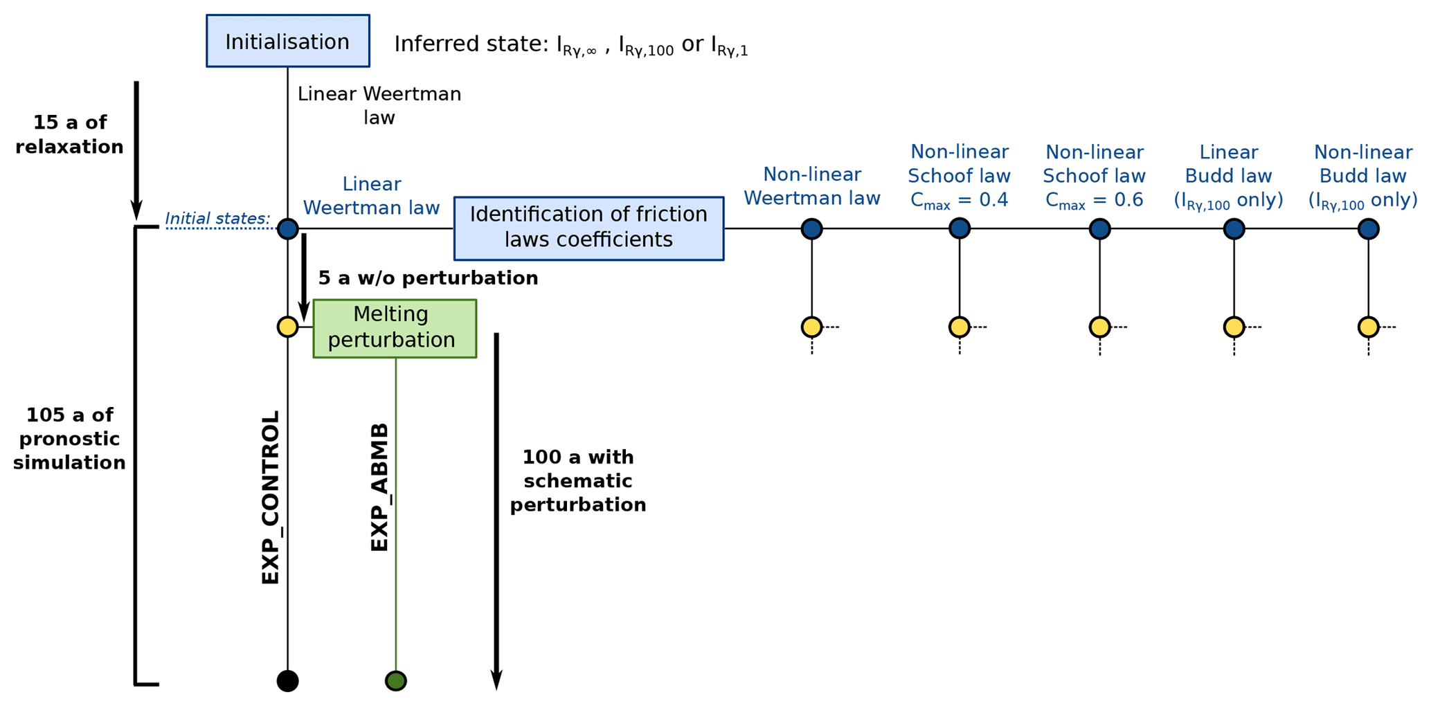
Figure 2 Flow chart summarising the consecutive steps of the present study for a given inferred state. The simulations EXP_CONTROL and EXP_ABMB are run for each of the five friction laws. The same procedure is repeated for each of the three inferred states, $I_{R_{\mathit{\gamma },\mathrm{\infty }}}$, $I_{R_{\mathit{\gamma },\mathrm{100}}}$ and $I_{R_{\mathit{\gamma },\mathrm{1}}}$, except that the non-linear and linear Budd friction laws are applied only to the inferred state $I_{R_{\mathit{\gamma },\mathrm{100}}}$.

2.2.1 Initialisation

A number of observations are used in order to initialise the model. The initial ice thickness is taken from Bedmap2 (Fretwell et al., 2013). A two-dimensional reference field of ${\stackrel{\mathrm{‾}}{\mathit{\eta }}}_{\mathrm{0}}$, denoted by ${\stackrel{\mathrm{‾}}{\mathit{\eta }}}_{\mathrm{0},\text{ref}}$, is computed using a three-dimensional ice temperature field of Antarctica (Brice Van Liefferinge, personal communication, 2016) obtained using a thermo-mechanical model forced with a mean geothermal heat flux (Van Liefferinge and Pattyn, 2013). In addition, we use the observed surface velocities of Rignot et al. (2011) to invert for basal shear stress and ice rheology. These velocities are given on each node of a regular grid with a 450 m resolution, except in some regions, which are sometimes very wide, over which the information is missing. The estimated error in the norm of observed velocities ranges, depending on regions, between 1 and 17 m a⁻¹. These observations have been collected over periods spanning several years, which could potentially induce inconsistencies in regions where the flow features are evolving rapidly.

The flow solution u of the SSA Eq. () depends on both the basal shear stress field and the effective viscosity field. For simplicity, the initial basal shear stress field is computed with a linear Weertman law of which we infer the friction coefficient distribution ${\widehat{C}}_{\text{W}}$. Although ${\stackrel{\mathrm{‾}}{\mathit{\eta }}}_{\mathrm{0},\text{ref}}$ enables a first approximation of the effective viscosity, there are significant uncertainties regarding the temperature field used to derive this field as well as the parameters linking the rate factor of ice to its temperature. In addition, ice viscosity does not depend only on temperature but also on several other parameters including damage, anisotropy, water content, density, grain size and impurity content (Cuffey and Paterson, 2010). Therefore, the question is whether the local discrepancies between observed and modelled velocities at any given point of the domain should be attributed to an inappropriate basal shear stress field or to errors on the reference field ${\stackrel{\mathrm{‾}}{\mathit{\eta }}}_{\mathrm{0},\text{ref}}$. Indeed, several model states consistent with observations can be constructed, for which the fit between modelled and observed velocities is obtained by adjusting the basal shear stress and the viscosity. In order to assess the sensitivity of the results to the initialisation strategy, we construct three inferred states – denoted by $I_{R_{\mathit{\gamma },\mathrm{\infty }}}$, $I_{R_{\mathit{\gamma },\mathrm{100}}}$ and $I_{R_{\mathit{\gamma },\mathrm{1}}}$ – by means of the control method, building on the approach described in Fürst et al. (2015).

The total cost function J_tot used for minimisation includes two cost functions and two Tikhonov regularisation terms:

$$\begin{array}{}\text{(15)}& J_{\text{tot}}=J_v+{\mathit{\lambda }}_{\text{div}}{J}_{\text{div}}+{\mathit{\lambda }}_{\text{reg},\mathit{\alpha }}{J}_{\text{reg},\mathit{\alpha }}+{\mathit{\lambda }}_{\text{reg},\mathit{\gamma }}{J}_{\text{reg},\mathit{\gamma }}.\end{array}$$

The misfit between modelled (u) and observed (u_obs) velocities is comprised in the first cost term J_v. To avoid errors due to interpolation of observed velocities at the model mesh nodes, J_v is a discrete sum evaluated directly at the observation points. It reads as follows:

$$\begin{array}{}\text{(16)}& J_{\text{v}}={\displaystyle \frac{\mathrm{1}}{\mathrm{2}}}\sum _{i=\mathrm{1}}^{N_{\text{obs}}}\left(\right|{\mathbf{u}}_{i,\text{obs}}-{\mathbf{u}}_i|{)}^{\mathrm{2}},\end{array}$$

where N_obs is the total number of available observations, u_i,obs is the velocity observed at point i, and u_i is the modelled velocity, which is interpolated at the observation point i. The second cost function J_div is intended to penalise the large gaps between ice flux divergence and mass balance, leading to inferred states closer to steady states. It reads as follows:

$$\begin{array}{}\text{(17)}& J_{\text{div}}={\displaystyle \frac{\mathrm{1}}{\mathrm{2}}}\underset{\mathrm{\Gamma }}{\int }{\left({\displaystyle \frac{\partial \left(uH\right)}{\partial x}}+{\displaystyle \frac{\partial \left(vH\right)}{\partial y}}-(a_{\text{s}}-a_{\text{b}})\right)}^{\mathrm{2}}\mathrm{d}\mathrm{\Gamma },\end{array}$$

where Γ is the model domain. During the inversion, we actually optimise the variables α and γ, which are related to the linear Weertman law coefficient and ${\stackrel{\mathrm{‾}}{\mathit{\eta }}}_{\mathrm{0}}$, respectively, as follows:

$$\begin{array}{}\text{(18)}& {\widehat{C}}_{\text{W}}={\mathrm{10}}^{\mathit{\alpha }},\end{array}$$

and

$$\begin{array}{}\text{(19)}& {\stackrel{\mathrm{‾}}{\mathit{\eta }}}_{\mathrm{0}}={\displaystyle \frac{{\mathit{\gamma }}^{\mathrm{2}}}{R_{\mathit{\gamma }}}}{\stackrel{\mathrm{‾}}{\mathit{\eta }}}_{\mathrm{0},\text{ref}},\end{array}$$

where R_γ is a constant. The variable changes (Eq. 18) and (Eq. 19) prevent non-physical negative values of basal shear stress and viscosity, respectively. In addition, the variable change (Eq. 19) enables us to tune the relative weight that will be put on basal shear stress and viscosity during inversion. Indeed, the minimisation of the cost functions relies on the calculation of their gradients with respect to the variables to optimise (MacAyeal, 1993). As a consequence, the higher the value attributed to R_γ, the lower the gradients of J_v and J_div calculated with respect to γ relative to the ones calculated with respect to α. In such a case, the distribution of α – and thus of the basal shear stress – will be more affected (on the grounded part only as τ_b is forced to zero wherever ice is floating) than for lower values of R_γ. The two regularisation functions J_reg,α and J_reg,γ in turn penalise first spatial derivatives of α and γ, respectively. They are meant to avoid overfitting the velocity observations and thus, improve the conditioning of the problem.

Among the three inferred states considered in this study, the two states $I_{R_{\mathit{\gamma },\mathrm{100}}}$ and $I_{R_{\mathit{\gamma },\mathrm{1}}}$ are constructed by optimising both α and γ with R_γ=100 and R_γ=1, respectively, in Eq. (19). Hence, more weight is put on basal shear stress to the detriment of viscosity for $I_{R_{\mathit{\gamma },\mathrm{100}}}$ than for $I_{R_{\mathit{\gamma },\mathrm{1}}}$. In contrast, the inferred state $I_{R_{\mathit{\gamma },\mathrm{\infty }}}$ is obtained by optimising α only, while ${\stackrel{\mathrm{‾}}{\mathit{\eta }}}_{\mathrm{0}}={\stackrel{\mathrm{‾}}{\mathit{\eta }}}_{\mathrm{0},\text{ref}}$. The gradients of J_tot are derived following the adjoint method (MacAyeal, 1993), while the minimisation itself is done using the quasi-Newton routine M1QN3 (Gilbert and Lemaréchal, 1989). The minimisation method being an iterative method, we need to provide initial guesses for the distributions of the variables to optimise. Following Morlighem et al. (2013), the initial guess for α is found by considering that, as a first approximation, the driving stress is exactly compensated by the basal shear stress at any given point of the ice–bed interface. Regarding the initial field of ${\stackrel{\mathrm{‾}}{\mathit{\eta }}}_{\mathrm{0}}$, it is simply set to ${\stackrel{\mathrm{‾}}{\mathit{\eta }}}_{\mathrm{0},\text{ref}}$ for both $I_{R_{\mathit{\gamma },\mathrm{100}}}$ and $I_{R_{\mathit{\gamma },\mathrm{1}}}$.

For each of the three inferred states, we follow a L-curve approach as described in Fürst et al. (2015) to retrieve the optimal values of λ_div, λ_reg,α and λ_reg,γ (only for $I_{R_{\mathit{\gamma },\mathrm{100}}}$ and $I_{R_{\mathit{\gamma },\mathrm{1}}}$), leading to inferred states showing good compromise between smooth distributions of α and γ, low differences between ice fluxes and mass balance and a good fit between observed and modelled velocities. We find $(\mathrm{5.1}\times {\mathrm{10}}^{-\mathrm{5}}$, 7.1×10⁵) for $I_{R_{\mathit{\gamma },\mathrm{\infty }}}$, $(\mathrm{5.9}\times {\mathrm{10}}^{-\mathrm{5}}$, 2.5×10⁶, 1.4×10⁶⁾ for $I_{R_{\mathit{\gamma },\mathrm{100}}}$, and $(\mathrm{1.8}\times {\mathrm{10}}^{-\mathrm{5}}$, 5.4×10⁶, 4.7×10⁵) for $I_{R_{\mathit{\gamma },\mathrm{1}}}$.

Although strong discrepancies between mass balance and ice flux are penalised through J_div in Eq. (15), the three inferred states are not exactly steady states. Seroussi et al. (2011) and Gillet-Chaulet et al. (2012) have reported the occurrence of non-physical ice thickness rates of change in the first years following the inversion. These ice flux anomalies are due to uncertainties in the model initial conditions, in particular regarding the prescribed topography and the values attributed to the various parameters, and are usually dissipated within a few years. For this reason, each of the three inferred states undergoes a relaxation period, the duration of which is arbitrarily fixed to 15 years. These relaxations are performed with the direct model as described in Sect. 2.1, with the basal shear stress field being computed through the linear Weertman law (see Fig. 2).

2.2.2 Identification of friction laws coefficients

For each of the three inferred states, the 15-year relaxation period leads to a new state characterised by a new velocity field, which we denote by ${\widehat{\mathbf{u}}}_{\text{b}}$, as well as a new basal shear stress field, denoted by ${\widehat{\mathit{\tau }}}_{\text{b}}$. These two fields relate to each other through the linear Weertman law, i.e. Eq. (5) with the inferred friction coefficient ${\widehat{C}}_{\text{W}}$ (which depends on the considered inferred state) and m=1. As thoroughly described in Brondex et al. (2017), these two fields can be used to analytically identify the distribution of the friction coefficient of other laws, which would lead to the same reference basal shear stress field ${\widehat{\mathit{\tau }}}_{\text{b}}$. Thus, the distributions of the friction coefficient of the non-linear Weertman law, the two Budd laws and the two Schoof laws can be identified by respectively solving the following:

$$\begin{array}{}\text{(20)}& C_{\text{W,nl}}={\widehat{C}}_{\text{W}}|{\widehat{\mathbf{u}}}_{\text{b}}{|}^{\mathrm{1}-m},\end{array}$$

$$\begin{array}{}\text{(21)}& C_{\text{B}}={\widehat{C}}_{\text{W}}{\displaystyle \frac{|{\widehat{\mathbf{u}}}_{\text{b}}{|}^{\mathrm{1}-m}}{\widehat{N}}},\end{array}$$

and,

$$\begin{array}{}\text{(22)}& C_{\text{S}}={\displaystyle \frac{\left|{\widehat{\mathit{\tau }}}_{\text{b}}\right|}{|{\widehat{\mathbf{u}}}_{\text{b}}{|}^m{\left(\mathrm{1}-{\left(\frac{\left|{\widehat{\mathit{\tau }}}_{\text{b}}\right|}{C_{\text{max}}\widehat{N}}\right)}^{\mathrm{1}/m}\right)}^m}}.\end{array}$$

For the Budd and Schoof laws, the effective pressure field $\widehat{N}$ used for the identification is calculated through Eq. (8) from the geometry obtained at the end of the relaxation period. Note that the fields ${\widehat{C}}_{\text{W}}$, ${\widehat{\mathbf{u}}}_{\text{b}}$, ${\widehat{\mathit{\tau }}}_{\text{b}}$ and $\widehat{N}$ being dependent on the inferred state, these identifications are repeated for each one of the three inferred states, except for the linear and non-linear Budd laws for which the identifications have been done only for the case $I_{R_{\mathit{\gamma },\mathrm{100}}}$ (see Fig. 2). Equations (20) and (21) enable us to identify the friction coefficients of the non-linear Weertman law and the two Budd laws at every grounded node covered with ice. At floating nodes or in the very few places of the domain which are ice-free when identification is performed, these coefficients are arbitrarily fixed to $C_{\text{W,nl}}={\mathrm{10}}^{-\mathrm{6}}$ MPa m${}^{-\mathrm{1}/\mathrm{3}}$ a^1∕3 and $C_{\text{B}}={\mathrm{10}}^{-\mathrm{6}}$ m${}^{-\mathrm{1}/\mathrm{3}}$ a^1∕3, respectively. This choice does not appear to be critical as all the following prognostic experiments lead exclusively to a GL retreat.

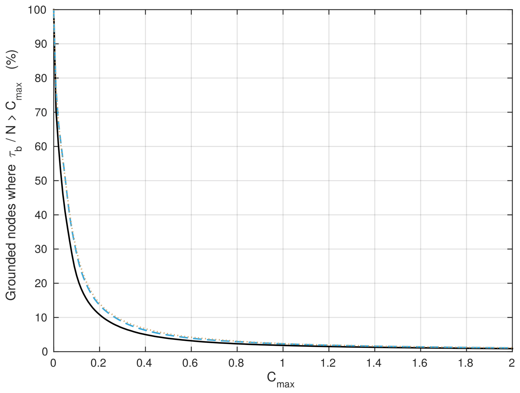
Figure 3 Percentage of grounded nodes where Iken's bound is not satisfied as a function of the value attributed to the parameter C_max for the inferred states $I_{R_{\mathit{\gamma },\mathrm{\infty }}}$ (black solid line), I_Rγ,100 (blue dashed line) and I_Rγ,1 (brown dotted line).

In contrast, because the Schoof law was constructed so that Iken's bound is satisfied (Schoof, 2005), Eq. (22) has a solution only in places where $\left|{\widehat{\mathit{\tau }}}_{\text{b}}\right|/\widehat{N}<C_{\text{max}}$. Figure 3 shows, for each of the three inferred states, the percentage of grounded nodes where the value of C_S cannot be identified directly from Eq. (22), depending on the value attributed to the parameter C_max. Although we do not expect the parameter C_max to be uniform all over the model domain, there is currently no way to constrain its spatial distribution. As a consequence, two different uniform values are considered: C_max=0.4 and C_max=0.6. Note that the identification of C_S then has to be done for each of the two values of C_max. Because the sensitivity of basal shear stress to C_S is very small in places close to flotation, the identification of C_S from Eq. (22) is only done at nodes where $\left|{\widehat{\mathit{\tau }}}_{\text{b}}\right|/\widehat{N}\le \mathrm{0.8}{C}_{\text{max}}$. The values of C_S at nodes where $\left|{\widehat{\mathit{\tau }}}_{\text{b}}\right|/\widehat{N}>\mathrm{0.8}{C}_{\text{max}}$ are linearly interpolated from the closest neighbouring nodes. In addition, we arbitrarily set $C_{\text{S}}={\mathrm{10}}^{-\mathrm{3}}$ MPa m${}^{-\mathrm{1}/\mathrm{3}}$ a^1∕3 in places which are ice-free or where ice is afloat when the identification is performed. Finally, we end up with six different distributions of C_S corresponding to the two values of C_max applied to the three inferred states $I_{R_{\mathit{\gamma },\mathrm{\infty }}}$, I_Rγ,100 and I_Rγ,1. For these six distributions, the percentage of grounded nodes at which C_S has to be interpolated is comprised between ∼4 % (for the initial state $I_{R_{\mathit{\gamma },\mathrm{\infty }}}$ associated with the parameter C_max=0.6) and ∼8 % (for the initial state I_Rγ,1 associated with the parameter C_max=0.4). As expected, the nodes at which an interpolation is required are the closest to flotation and, therefore, are mostly located directly upstream of the GL.

As stated previously, the identification steps lead to 14 different initial states, which are used as the starting points of the prognostic simulations (blue dots in Fig. 2).

2.2.3 Prognostic simulations

The 14 initial states are then run forward in time for 105 years under two different scenarios: (1) a control run (EXP_CONTROL) and (2) a basal melt anomaly run (EXP_ABMB). The EXP_CONTROL run is an unforced forward experiment aiming to characterise model drift, which depends both on the initial state and the friction law. Therefore, all model parameters and forcing in EXP_CONTROL are the same as those used for initialisation and presented in Sect. 2.1.

The EXP_ABMB run consists of applying a synthetic anomaly of basal melting rate under floating ice, all other model parameters and forcing being kept the same as in EXP_CONTROL: after a first 5-year period free of any perturbation, a uniform basal melting rate anomaly “abmb” of 13.2 m a⁻¹ is progressively added to the initial basal melting rate a_b, given by Eq. (14), over the following 40 years of simulation. Thus, the basal melting rate a_b,ABMB for this run is given by

$$\begin{array}{}\text{(23)}& \left\{\begin{array}{ll}{a}_{\text{b,ABMB}}=a_{\text{b}}& \text{if}\mathrm{0}\le t<\mathrm{5}\text{a}\\ a_{\text{b,ABMB}}=a_{\text{b}}+\text{abmb}{\displaystyle \frac{\text{floor}\left(t\right)-\mathrm{5}}{\mathrm{40}}}& \text{if}\mathrm{5}\le t<\mathrm{45}\text{a}\\ a_{\text{b,ABMB}}=a_{\text{b}}+\text{abmb}& \text{if}t\ge \mathrm{45}\text{a}.\end{array}\right.\end{array}$$

The basal melting rate anomaly abmb corresponds to the one prescribed for the ASE within the InitMIP-Antarctica framework (Nowicki et al., 2016).

3 Results

3.1 Initialisation

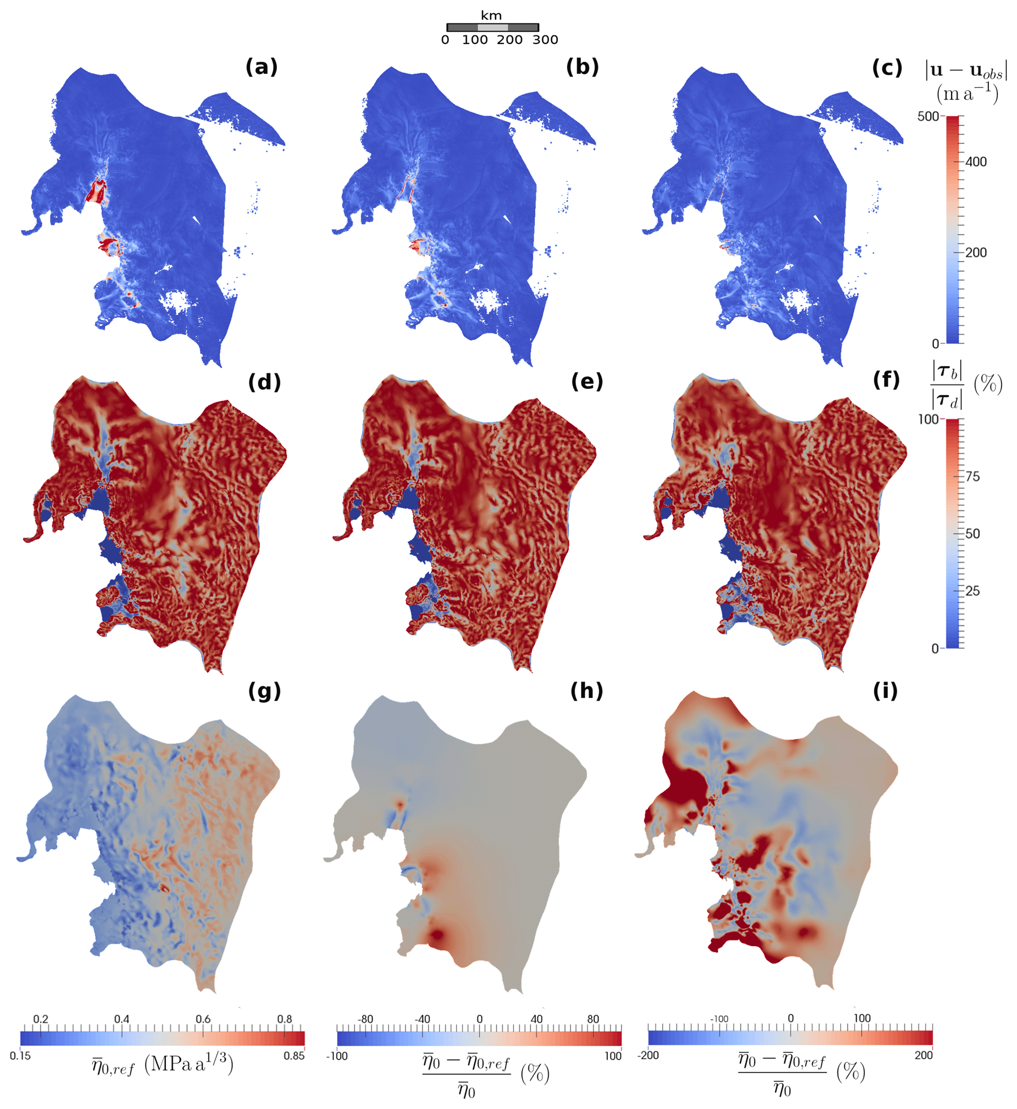
Figure 4 Comparison of inferred states $I_{R_{\mathit{\gamma },\mathrm{\infty }}}$ (first column), $I_{R_{\mathit{\gamma },\mathrm{100}}}$ (second column) and $I_{R_{\mathit{\gamma },\mathrm{1}}}$ (third column). For each of the three inferred states, the first row – panels (a), (b) and (c) – shows the absolute difference between modelled u and observed u_obs velocities (m a⁻¹); the second row – panels (d), (e) and (f) – shows the ratio of the norm of τ_b relatively to the norm of τ_d; the third row shows the reference field ${\stackrel{\mathrm{‾}}{\mathit{\eta }}}_{\mathrm{0},\text{ref}}$ (MPa a^1∕3) for the inferred state $I_{R_{\mathit{\gamma },\mathrm{\infty }}}$ – panel (g) – as well as the relative difference between ${\stackrel{\mathrm{‾}}{\mathit{\eta }}}_{\mathrm{0}}$ and ${\stackrel{\mathrm{‾}}{\mathit{\eta }}}_{\mathrm{0},\text{ref}}$ for the inferred states $I_{R_{\mathit{\gamma },\mathrm{100}}}$ (second column) and $I_{R_{\mathit{\gamma },\mathrm{1}}}$ – panels (h) and (i). Note the different colour scales for panels (h) and (i).

The three inferred states $I_{R_{\mathit{\gamma },\mathrm{\infty }}}$, $I_{R_{\mathit{\gamma },\mathrm{100}}}$ and $I_{R_{\mathit{\gamma },\mathrm{1}}}$ are compared in Fig. 4. The absolute difference between modelled u and observed u_obs velocities turns out to shrink when both basal shear stress and viscosity are inferred (Fig. 4a–c). This is particularly true for the ice shelves, which do not feel any basal shear stress: although the basal shear stress directly upstream of the GL do influence velocities within the downstream ice shelf, the most efficient way to obtain a better match between modelled and observed velocities in floating areas is through a local adjustment of viscosity. Thus, the inferred state $I_{R_{\mathit{\gamma },\mathrm{\infty }}}$ shows important errors on Pine Island, Thwaites and, to a lesser extent, Crosson ice shelves (Fig. 4a). The root mean squared (rms) errors obtained for the inferred states $I_{R_{\mathit{\gamma },\mathrm{\infty }}}$, $I_{R_{\mathit{\gamma },\mathrm{100}}}$ and $I_{R_{\mathit{\gamma },\mathrm{1}}}$ are 85.5, 52.4 and 37.5 m a⁻¹.

The ratio between the norm of the basal shear stress and the norm of the driving stress is shown in Fig. 4d–f. In addition, plots of the norm of the basal shear stress obtained for the three inferred states are included in the Supplement (Fig. S1) to allow for a comparison with previous work in which inversions of basal shear stress in the regions of PIG and Thwaites were performed (Joughin et al., 2009; Morlighem et al., 2010). At the end of the inversions, there are several regions where the local driving stress is not entirely compensated by the local basal shear stress (blue regions). As expected, these regions correspond to regions of rapid flow; in particular, Pine Island Ice Stream can be easily distinguished. The regions of low τ_b become narrower as more weight is put on viscosity during inversion. Indeed, when the viscosity is inferred, another way for the inversion algorithm to increase the modelled velocities in areas where they would be too low otherwise is to soften the ice locally: this is the case, for example, in the higher part of PIG, in particular for the inferred state $I_{R_{\mathit{\gamma },\mathrm{1}}}$ for which the inversion algorithm induces a local reduction in viscosity rather than of the basal stress to increase the modelled velocities (panels f and i of Fig. 4). It is also this same mechanism which is behind the low viscosity bands, easily distinguishable in Fig. 4h (note that they are also present in Fig. 4i but less visible due to the wider colour scale). These soft bands correspond to shear margins, where high shear stresses induce a local reduction of ice viscosity through different physical processes, including damage, strain heating and the development of crystalline fabric (Bondzio et al., 2017; Borstad et al., 2013; Minchew et al., 2018). On the contrary, the inversion algorithm can render the ice locally stiffer in order to decrease the modelled velocities in areas where they are too high compared to the observations, which is typically the case for ice shelves.

Because the model states obtained after the initialisation step are not steady states, they drift toward new states during the following 15-year relaxation period. Overall, the three inferred states show similar evolution patterns with relatively moderate ice thickness changes, except for the Pine Island and Thwaites ice shelves, where ice thickness increases by about 100 m over the 15 years. In contrast, ice streams become slightly thinner, losing a few tens of metres of ice in some places. At the end of the relaxation period, the thickness rates of change have decreased to physically acceptable values for all the inferred states, with, at most, 30 m a⁻¹ of absolute thickness rate of change, concentrated within very localised areas; elsewhere, ice thickness is nearly at equilibrium with, at most, a few m a⁻¹ of absolute thickness rate of change. Although the modelled velocity structure remains similar to observations, the rms errors between observed velocities and velocities computed at the end of the relaxation period have risen to 124.8, 119.4 and 96.4 m a⁻¹ for $I_{R_{\mathit{\gamma },\mathrm{\infty }}}$, $I_{R_{\mathit{\gamma },\mathrm{100}}}$ and $I_{R_{\mathit{\gamma },\mathrm{1}}}$, respectively.

3.2 Identification of friction laws coefficients

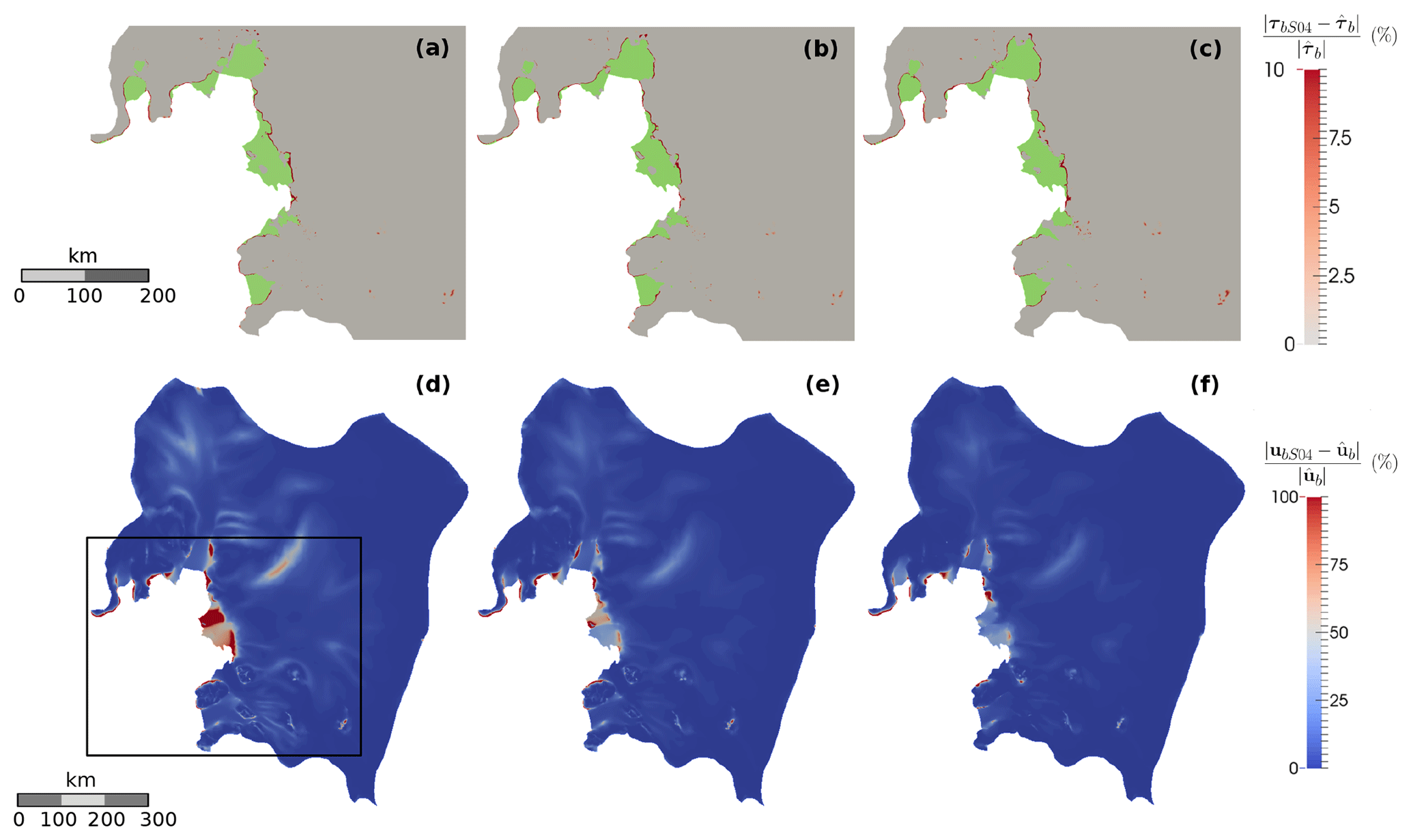
Figure 5 Relative differences (%) between the fields of τ_b (first row) and u_b (second row) produced by the linear Weertman law and the non-linear Schoof law associated with C_max=0.4 and the C_S distributions identified through Eq. (22) or interpolated, for the inferred states $I_{R_{\mathit{\gamma },\mathrm{\infty }}}$ – panels (a) and (d) –, $I_{R_{\mathit{\gamma },\mathrm{100}}}$ – panels (b) and (e) – and $I_{R_{\mathit{\gamma },\mathrm{1}}}$ – panels (c) and (f). Panels of the first row zoom into the neighbourhood of ice shelves (shown in green), where the relative differences in τ_b are concentrated, while panels on the second row show the whole ASE. The zoomed-in area is highlighted with a black box on panel (d).

For each of the three inferred states, the basal shear stress fields computed with the non-linear Weertman law and with the two Budd laws using the friction coefficient distributions deduced through Eqs. (20) and (21), respectively, are identical to the basal shear stress fields ${\widehat{\mathit{\tau }}}_{\text{b}}$ used for the identifications. In contrast, because the value of C_S cannot be exactly identified through Eq. (22) at every grounded node but needs to be interpolated in some places, ${\widehat{\mathit{\tau }}}_{\text{b}}$ is not perfectly reproduced with the Schoof law. Figure 5a–c show an enlargement of regions within which the relative differences between the basal shear stress field calculated with the non-linear Schoof law (7) associated with C_max=0.4 and the C_S distributions identified through Eq. (22) or interpolated, which is denoted by τ_bS04, and the reference basal shear stress fields ${\widehat{\mathit{\tau }}}_{\text{b}}$ are the highest. As expected, the highest relative differences are obtained close to the ice shelves (shown in green in Fig. 5a–c), where the nodes are close to flotation and C_S needs to be interpolated. Elsewhere, the fields of τ_b produced by the two friction laws are numerically identical. The relative difference between τ_bS04 and ${\widehat{\mathit{\tau }}}_{\text{b}}$ at nodes where C_S is interpolated rarely exceeds 10 %; higher differences (up to 100 %) occur very locally at some of the last grounded nodes. The results obtained with the parameter C_max=0.6 (not shown) are similar, except that the nodes where the interpolation of C_S is required are fewer and, therefore, the regions within which the relative difference between τ_bS06 and ${\widehat{\mathit{\tau }}}_{\text{b}}$ is not null are less extended. Note that in places where the relative difference is not null, the Schoof law systematically produces the weakest basal shear stress.

Although they are moderate and very localised, the differences between the basal shear stress fields computed with the linear Weertman law and the Schoof law induce significant differences on the recomputed velocity fields (Fig. 5d–f). These differences propagate from the regions showing the highest differences in terms of τ_b to the floating areas located directly downstream (particularly distinguishable on Thwaites Ice Shelf). Indeed, the decrease in the total basal shear stress due to the interpolation of C_S close to the GL needs to be compensated elsewhere so that the global stress balance keeps being satisfied. Because the floating areas do not support any basal shear stress, the perturbation is transmitted to the front of ice shelves, unless it can be compensated by an increase in the buttressing effect through a contact on a pinning point or an increase in lateral stresses at shear margins in the case of confined ice shelves. This latter mechanism is well illustrated in Fig. 5d–f, which shows an important increase in velocities at the shear margins of PIG when the linear Weertman law is replaced by the Schoof law. Furthermore, it turns out that the relative differences in the velocity field are more pronounced when more weight is put on basal shear stress during the initialisations. Indeed, when the inversion focuses on the basal shear stress field only (inferred state $I_{R_{\mathit{\gamma },\mathrm{\infty }}}$), the ice flow is more sensitive to any perturbation of this field. Once again, the results obtained with the parameter C_max=0.6 (not shown) are very similar with slightly lower relative differences between the velocity fields calculated with the two laws.

Finally, the identification (Eq. 22) being performed at mesh nodes, the Gaussian integration over elements induces small numerical errors on the recomputed velocity field. These numerical errors are concentrated in coarse-mesh areas and correspond to the discrepancies of, at most, a few tens of percents observed further inland, in places where the differences in terms of τ_b are null (Fig. 5d–f). Similar numerical errors are observed within the same areas when the velocity fields produced with the non-linear Weertman law and the two Budd laws after the identification step are compared to ${\widehat{\mathbf{u}}}_{\text{b}}$.

3.3 Prognostic simulations

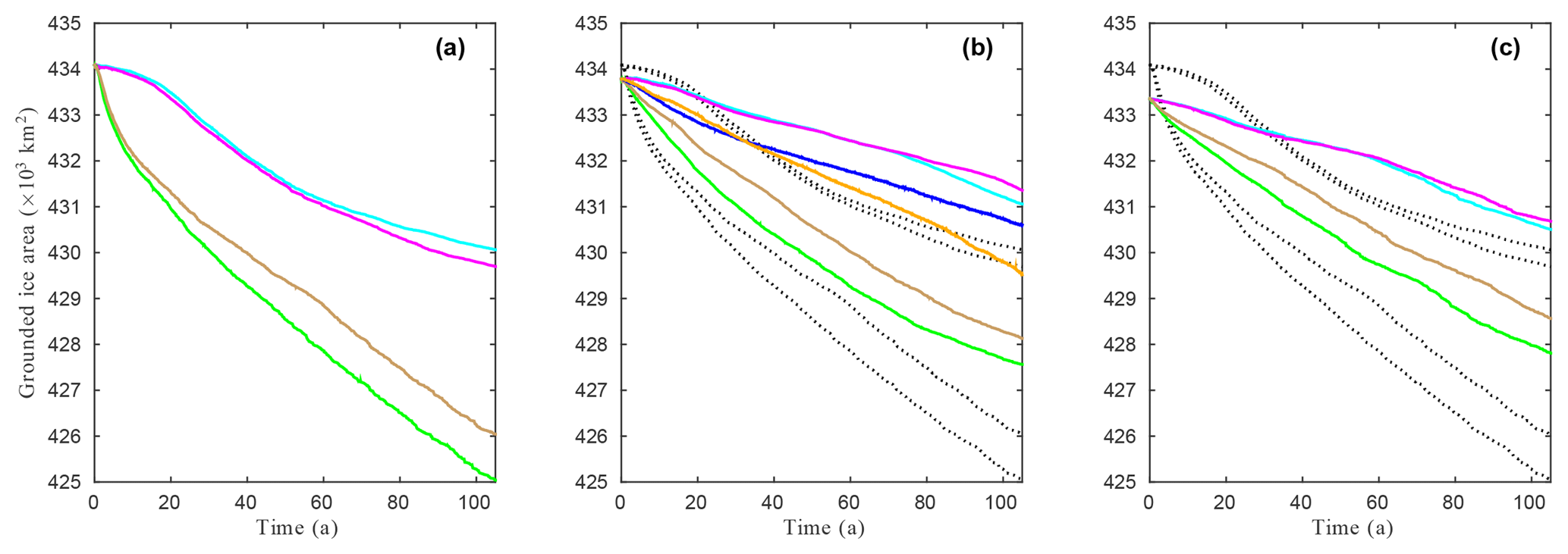
Figure 6 Evolution of grounded ice area (×10³ km²) as a function of time during EXP_CONTROL for the inferred states (a) $I_{R_{\mathit{\gamma },\mathrm{\infty }}}$, (b) $I_{R_{\mathit{\gamma },\mathrm{100}}}$ and (c) $I_{R_{\mathit{\gamma },\mathrm{1}}}$ and the friction laws, linear Weertman (cyan), non-linear Weertman (magenta), Schoof with C_max=0.4 (green), Schoof with C_max=0.6 (brown), linear Budd (orange, for the initial state $I_{R_{\mathit{\gamma },\mathrm{100}}}$ only) and non-linear Budd (blue, for the initial state $I_{R_{\mathit{\gamma },\mathrm{100}}}$ only). The results obtained with the various friction laws for the inferred state $I_{R_{\mathit{\gamma },\mathrm{\infty }}}$ are reported on (b) and (c) for ease of comparison (black dotted lines).

The evolution of the grounded ice area during the control run for the three inferred states and the various friction laws is shown in Fig. 6. A decrease (resp. an increase) in the grounded ice area reflects a retreat (resp. an advance) of the GL. After relaxation, the grounded ice area at t=0 a differs depending on the considered inferred state: it ranges between 433 400 km² for $I_{R_{\mathit{\gamma },\mathrm{1}}}$ and 434 000 km² for $I_{R_{\mathit{\gamma },\mathrm{\infty }}}$.

Irrespective of the chosen inferred state or friction law, the natural (i.e. unperturbed) evolution of the domain is toward a reduction of its grounded ice area: the Schoof law with C_max=0.4 systematically gives the more pronounced GL retreat with a reduction of grounded ice area over the 105a of the control run ranging between 5000 km² for $I_{R_{\mathit{\gamma },\mathrm{1}}}$ and 7700 km² for $I_{R_{\mathit{\gamma },\mathrm{\infty }}}$. In contrast, the reduction of the grounded ice area obtained with the non-linear Weertman law ranges between 2400 km² for $I_{R_{\mathit{\gamma },\mathrm{100}}}$ and 4300 km² for $I_{R_{\mathit{\gamma },\mathrm{\infty }}}$. Note that the evolutions of the grounded ice area obtained with the two Weertman laws are very close to one another over the entire 105 a of the control run, while the two Schoof laws produce noticeably different evolutions from the beginning of the run, with the case C_max=0.6 showing less GL retreat than the case C_max=0.4. This could be partly due to the differences between ${\widehat{\mathbf{u}}}_{\text{b}}$ and the velocity field recomputed with the Schoof law after initialisation, which are lower for C_max=0.6 than for C_max=0.4 as reported in Sect. 3.2. For the inferred state $I_{R_{\mathit{\gamma },\mathrm{100}}}$, the Budd laws produce intermediate results with a reduction of the grounded ice area of 3000 km² for the non-linear Budd law and of 4200 km² for the linear Budd law.

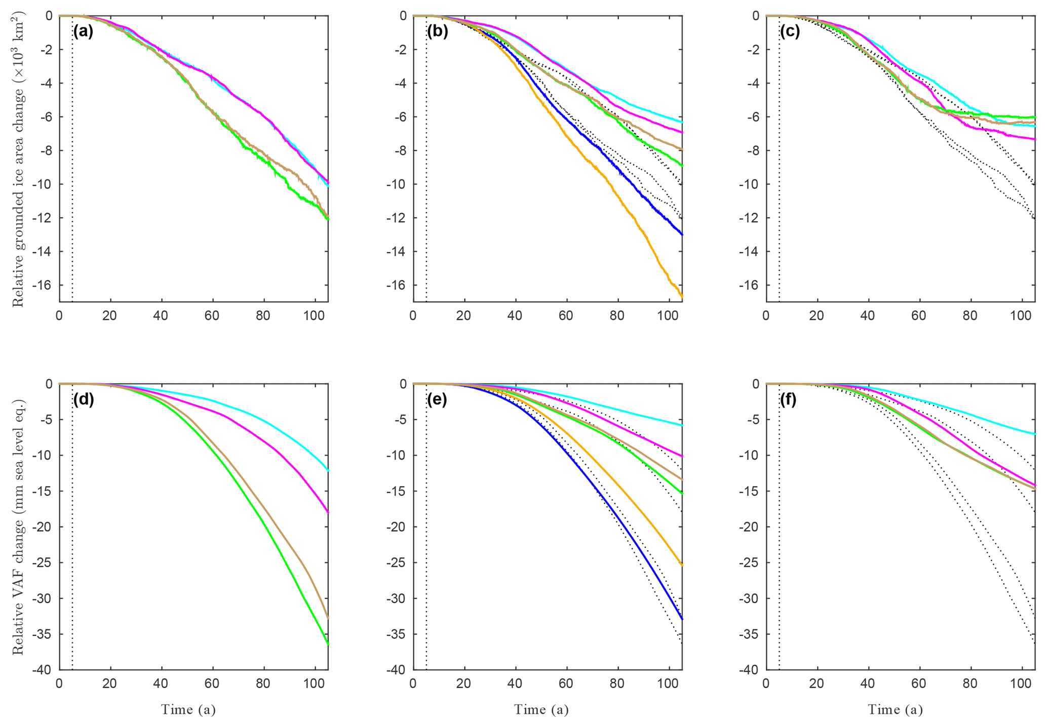
Figure 7 Evolution of grounded ice area in ×10³ km² (first row) and of volume above flotation in millimetre sea-level equivalent (second row) as a function of time during EXP_ABMB (coloured solid lines) relative to EXP_CONTROL for the inferred states $I_{R_{\mathit{\gamma },\mathrm{\infty }}}$ – panels (a) and (d), $I_{R_{\mathit{\gamma },\mathrm{100}}}$ – panels (b) and (e), and $I_{R_{\mathit{\gamma },\mathrm{1}}}$ – panels (c) and (f) – with the friction laws, linear Weertman (cyan), non-linear Weertman (magenta), Schoof with C_max=0.4 (green), Schoof with C_max=0.6 (brown), linear Budd (orange, for the inferred state $I_{R_{\mathit{\gamma },\mathrm{100}}}$ only) and non-linear Budd (blue, for the inferred state $I_{R_{\mathit{\gamma },\mathrm{100}}}$ only). The results obtained with the various friction laws for the inferred state $I_{R_{\mathit{\gamma },\mathrm{\infty }}}$ are reported on, respectively, (b–c) and (e–f) for ease of comparison (black dotted lines). The vertical black dotted lines mark the introduction of the perturbation at t=5 a.

The results of the perturbation experiments EXP_ABMB are shown relative to the control simulation EXP_CONTROL (Fig. 7). We consider both the relative reductions of grounded ice area as well as the relative losses of volume above flotation (VAF), given in millimetres of sea-level equivalent (SLE). For the inferred state $I_{R_{\mathit{\gamma },\mathrm{\infty }}}$, the grounded ice areas produced by the two Weertman laws at the end of EXP_ABMB are about 2000 km² larger than the ones produced by the two Schoof laws. The difference between the linear and non-linear Weertman laws or between the two Schoof laws (C_max=0.4 and C_max=0.6) is about 10 times smaller (∼200 km²). However, the differences in terms of VAF change are more significant with 6mm SLE of difference between the two Weertman laws and 3mm SLE of difference between the two Schoof laws. For comparison, the linear Weertman law and the Schoof law with C_max=0.4 show 24 mm SLE of difference in terms of VAF loss at the end of EXP_ABMB. When the viscosity is adjusted during inversion (cases $I_{R_{\mathit{\gamma },\mathrm{100}}}$ and $I_{R_{\mathit{\gamma },\mathrm{1}}}$), the GL shows less retreat and the relative VAF losses are less important (Fig. 7b–c and e–f). In addition, the relative evolutions of VAF obtained with the Weertman laws are closer to the ones obtained with the Schoof laws, except for the experiment associated with the inferred state $I_{R_{\mathit{\gamma },\mathrm{1}}}$ and the linear Weertman law (Fig. 7e–f). Note that the Schoof laws produce more GL retreat and more SLR contribution than the Weertman laws for the inferred states $I_{R_{\mathit{\gamma },\mathrm{\infty }}}$ and $I_{R_{\mathit{\gamma },\mathrm{100}}}$. On the contrary, for the inferred state $I_{R_{\mathit{\gamma },\mathrm{1}}}$, the grounded ice areas seem to stabilise around t=60 a with the Schoof laws, while they keep decreasing for a few more years with the Weertman laws, so that the grounded ice areas obtained with the two latter at the end of EXP_ABMB are slightly smaller than the ones obtained with the two former. Despite a very similar decrease in terms of grounded ice areas to the ones obtained with the two Schoof laws, the linear Weertman law predicts 8 mm SLE less VAF loss (Fig. 7f). For the inferred state $I_{R_{\mathit{\gamma },\mathrm{100}}}$, the two Budd friction laws show much stronger responses to the basal melting rate perturbation than the four other laws: at the end of EXP_ABMB, it results in a grounded ice area reduction comprised between 13 000 km² for the non-linear Budd law and 16 600 km² for the linear Budd law relative to EXP_CONTROL, while the grounded ice area reduction ranges between 6300 and 8900 km² for the four other experiments. Likewise, the relative VAF loss obtained at the end of EXP_ABMB is 25 mm SLE for the linear Budd law and 33 mm SLE for the non-linear Budd law, whereas it ranges between 6 and 15 mm SLE for the other experiments. This dramatic response of the GL dynamics to the perturbation when a Budd law is used is in line with the results reported in Brondex et al. (2017).

Figure 8 Bed elevation (m) and GL positions at the end of the experiment EXP_ABMB for the inferred states, (a) $I_{R_{\mathit{\gamma },\mathrm{\infty }}}$, (b) $I_{R_{\mathit{\gamma },\mathrm{100}}}$ and (c) $I_{R_{\mathit{\gamma },\mathrm{1}}}$, and the friction laws, linear Weertman (cyan), non-linear Weertman (magenta), Schoof with C_max=0.4 (green), Schoof with C_max=0.6 (brown), linear Budd (orange, for the inferred state $I_{R_{\mathit{\gamma },\mathrm{100}}}$ only) and non-linear Budd (blue, for the inferred state $I_{R_{\mathit{\gamma },\mathrm{100}}}$ only). The GL position at t=0 a is reported for each of the three inferred states (solid black lines). The solid white lines in (b) correspond to flow lines at which ice-sheet profiles are represented in Fig. 9.

The GL positions obtained with the various initial states at the beginning and at the end of experiment EXP_ABMB are represented in Fig. 8. The GL produced with the two Schoof laws are almost systematically more retreated than the ones produced with the two Weertman laws. On the other hand, the GL final positions obtained with the Schoof law associated with C_max=0.6 (brown solid lines) are generally very close to the ones obtained with the Schoof law associated with C_max=0.4 (green solid lines). Likewise, the GL final positions obtained with the linear Weertman law (cyan solid lines) are often very close to the ones obtained with the non-linear Weertman law (magenta solid lines), except for the inferred state $I_{R_{\mathit{\gamma },\mathrm{\infty }}}$, where the former is sometimes more advanced and sometimes more retreated than the latter. Note that this does not contradict the previously mentioned result regarding the similar evolution of grounded ice areas obtained with the two Weertman laws for $I_{R_{\mathit{\gamma },\mathrm{\infty }}}$, as evolutions represented in Fig. 7 are relative to EXP_CONTROL, while the GL positions reported in Fig. 8 are absolute. The spatial distribution of the GL retreat is primarily controlled by the bed topography, as already reported by Seroussi et al. (2017). As a consequence, the Schoof and Weertman laws all give the same retreat patterns: the most pronounced retreats are observed in regions of gentle slope (particularly visible upstream of the Thwaites Ice Shelf), while the GL tends to wrap around prominences. However, for $I_{R_{\mathit{\gamma },\mathrm{100}}}$, the patterns of GL retreat obtained with the Budd laws are significantly different from the ones obtained with the four other laws. Indeed, the final GL position obtained with the non-linear Budd law is the most advanced in the Thwaites region, where the other laws (especially the Schoof laws and the linear Budd law) induce important retreats. On the contrary, both the linear and non-linear Budd laws induce retreats of several tens of kilometres in the regions of Cosgrove and Dotson ice shelves, where the four other laws give very similar final GL positions with limited retreat (especially in the Cosgrove Ice Shelf region).

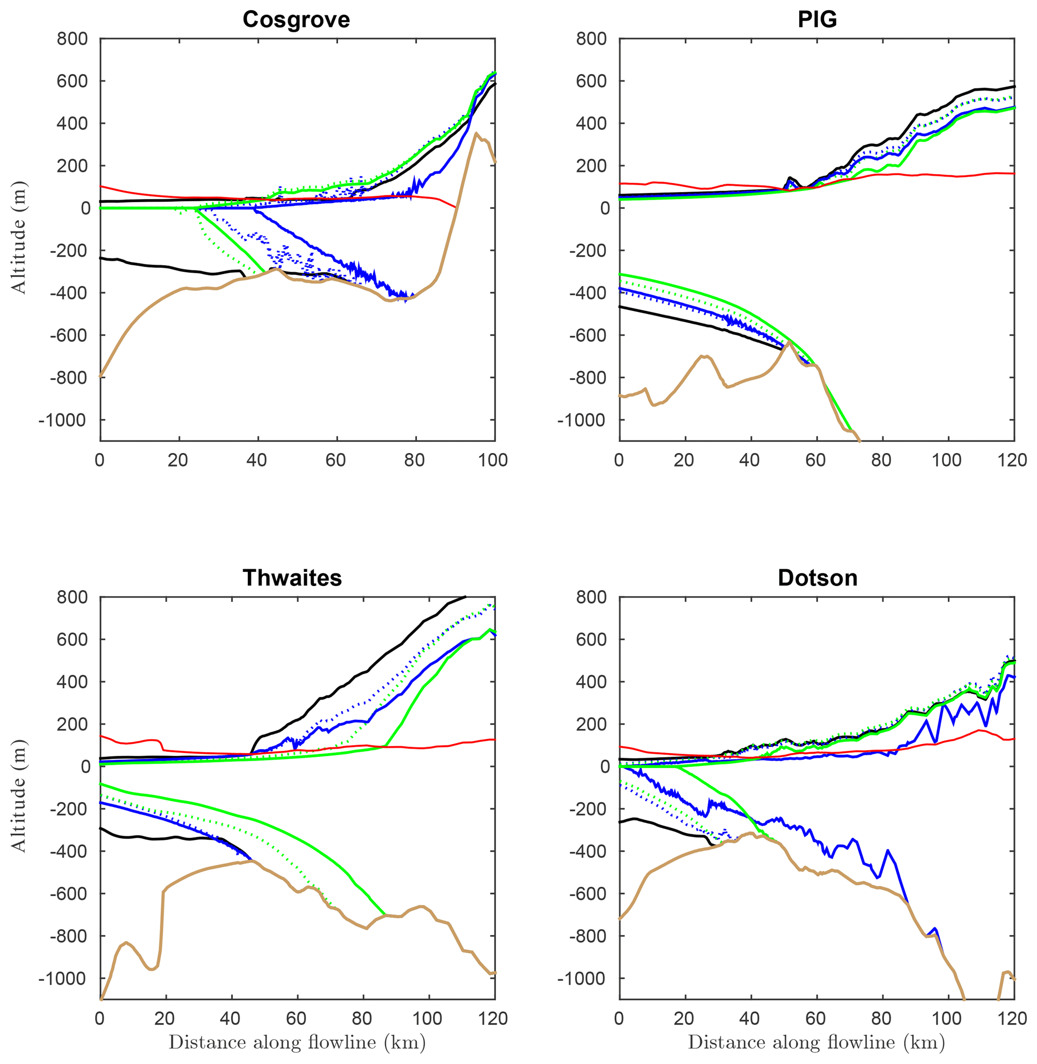
Figure 9 Ice-sheet profiles obtained for the inferred state $I_{R_{\mathit{\gamma },\mathrm{100}}}$ at t=0 a (black solid line), t=55 a (coloured dotted line) and t=105 a (coloured solid line) of EXP_ABMB with the Schoof law associated with C_max=0.4 (green) and the non-linear Budd law (blue), along the flow lines reported in Fig. 8. The solid light-brown line is the bed elevation. The red solid line is the flotation altitude z_f, given by $z_{\text{f}}=(\mathrm{1}-{\mathit{\rho }}_w/{\mathit{\rho }}_{\text{i}})b$.

The initial and final ice-sheet profiles obtained with the Schoof and non-linear Budd laws are represented in Fig. 9, along four selected flow lines (reported in white in Fig. 8b). By definition, wherever ice is grounded, the ice thickness comprised between z_s and the flotation altitude z_f, given by $z_{\text{f}}=(\mathrm{1}-{\mathit{\rho }}_w/{\mathit{\rho }}_{\text{i}})b$, constitutes the thickness above flotation. Because the GL position is deduced from Eq. (11), it is located at the exact vertical of the point where z_s=z_f. Looking at the initial profiles, it turns out that the initial ice thickness above flotation increases rapidly upstream of the GL for the PIG and Thwaites flow lines. On the contrary, it increases very progressively as we go further upstream within the grounded part for the Dotson flow line and even more so for the Cosgrove flow line. For all the considered flow lines, the bed profiles have sections of retrograde slope susceptible to giving rise to a MISI, unless this can be prevented by sufficient lateral buttressing (Gudmundsson et al., 2012). A MISI seems to occur for the Cosgrove and Dotson flow lines when the non-linear Budd law is used and for the PIG and Thwaites flow lines when the Schoof law is used. Note that the ice shelves of Cosgrove and Dotson have completely disappeared at the end of EXP_ABMB with both the Schoof and Budd laws. On the contrary, whatever the chosen law, PIG and Thwaites ice shelves are conserved until the end of the experiment, although they become thinner. A similar figure comparing the profiles obtained with the linear and non-linear Budd laws is available in the Supplement (Fig. S2).

4 Discussion

Among the three inferred states, $I_{R_{\mathit{\gamma },\mathrm{100}}}$ appears to be the most physically acceptable one, despite an rms error that is slightly higher than the one obtained for $I_{R_{\mathit{\gamma },\mathrm{1}}}$. Indeed, for $I_{R_{\mathit{\gamma },\mathrm{100}}}$, the inferred ${\stackrel{\mathrm{‾}}{\mathit{\eta }}}_{\mathrm{0}}$ has been reduced, at most, by 84 % (at the shear margins) and increased, at most, by 144 % (very locally in the higher part of the Kohler Glacier, which feeds the Dotson Ice Shelf) compared to the reference field ${\stackrel{\mathrm{‾}}{\mathit{\eta }}}_{\mathrm{0},\text{ref}}$. In contrast, for $I_{R_{\mathit{\gamma },\mathrm{1}}}$, ${\stackrel{\mathrm{‾}}{\mathit{\eta }}}_{\mathrm{0}}$ is at least 3 times higher than ${\stackrel{\mathrm{‾}}{\mathit{\eta }}}_{\mathrm{0},\text{ref}}$ on large parts of the domain and more than 15 times higher in some very localised areas close to the Kohler Glacier (regions in red in Fig. 4i). Without considering any of the other parameters affecting the ice viscosity, such an increase could only be explained by a reduction of the ice temperature of several tens of degrees Celsius (up to 50 ^∘C in some regions) compared to the reference temperature field. On the other hand, even if ice was assumed to be at the melting point, the viscosity reduction observed in some other parts of the domain (regions in blue in Fig. 4i) is non-physical. Note that for $I_{R_{\mathit{\gamma },\mathrm{100}}}$, an increase in the ice temperature of a few degrees only relative to the reference temperature field is sufficient to explain the local reduction of ice viscosity observed in some regions (much less extended than for $I_{R_{\mathit{\gamma },\mathrm{1}}}$) after the inversion, except at the shear margins where the low viscosity bands can be attributed to the presence of damaged ice and/or to strain heating and/or to anisotropy. Finally, the difference between modelled and observed velocities, especially on the ice shelves, are too high for the inferred state $I_{R_{\mathit{\gamma },\mathrm{\infty }}}$.

The basal melting rate increase prescribed for the perturbation experiments EXP_ABMB induces a thinning of the ice shelves, which reduces their buttressing effect and causes a retreat of the GL. The amplitude of this retreat increases as more weight is put on basal shear stress to the detriment of viscosity during initialisation. Indeed, adjusting viscosity during initialisation leads to low viscosity bands at shear margins, which hamper the transfer of lateral stresses toward the interior of ice shelves and, from there, toward the ice streams which feed them. It follows that the model states for which viscosity is inferred are less sensitive to a reduction of the buttressing effect as the contribution of this effect to the initial global stress balance is less important than for $I_{R_{\mathit{\gamma },\mathrm{\infty }}}$.

The different friction laws show different sensitivities to velocity and effective pressure – from no explicit dependence on N for the Weertman laws to an explicit dependence over the whole domain for the Budd laws – which leads to different evolutions of basal shear stress as the geometry of the domain evolves in response to the perturbation. Therefore, it is not surprising that, overall, grounded ice area evolutions and VAF losses show more sensitivity to the chosen friction law when more weight is put on basal shear stress to the detriment of viscosity during initialisation, i.e. for $I_{R_{\mathit{\gamma },\mathrm{\infty }}}$ than for $I_{R_{\mathit{\gamma },\mathrm{100}}}$ or $I_{R_{\mathit{\gamma },\mathrm{1}}}$. The choice of the friction law affects not only the grounded ice area evolution, but also the evolution of the ice thickness. Thus, the grounded ice area shrinkage is more pronounced when using the linear Budd law rather than the non-linear Budd law, whereas the latter induces more VAF loss than the former. Similarly, although the linear and non-linear Weertman laws lead to similar evolutions of the grounded ice area for $I_{R_{\mathit{\gamma },\mathrm{\infty }}}$, they produce significantly different VAF losses. The Weertman laws systematically predict the lowest VAF losses. In addition, as for the Budd laws, the linear Weertman law always predicts less VAF loss than the non-linear Weertman law, which is in line with the results of Ritz et al. (2015), showing a higher contribution of the Antarctic ice sheet to SLR as the Weertman law tends toward a perfectly plastic law, i.e. m→0 in Eq. (5). The two Schoof laws lead to significantly higher VAF losses than the Weertman laws, with one exception: the non-linear Weertman law for the inferred state $I_{R_{\mathit{\gamma },\mathrm{1}}}$, which predicts a VAF loss very close to the ones obtained with the two Schoof laws. This is likely due to the fact that, for $I_{R_{\mathit{\gamma },\mathrm{1}}}$, there are several regions of unexpectedly high viscosity located a few tens of kilometres upstream of the initial GL (Fig. 4i). Once the GL has reached these regions, ice is stiffer and hampers further retreat, which explains the stabilisation of the grounded ice area seen in Fig. 7c. As a consequence, the rate of VAF losses obtained with the two Schoof laws decreases, which also occurs with the non-linear Weertman law but later on, so that, at the end of EXP_ABMB, the relative VAF losses predicted by the three laws are almost identical. On the other hand, for the Schoof law, the lower the value of C_max, the higher the predicted VAF losses. This is not surprising as the regions over which friction is governed by a Coulomb regime when using a Schoof law widen when the value of C_max decreases (Brondex et al., 2017). For $I_{R_{\mathit{\gamma },\mathrm{100}}}$, the VAF losses obtained with the two Budd laws are dramatically higher than the one obtained with the four other laws, which is in line with the results obtained in Brondex et al. (2017).

The sensitivity of ice thickness rates of change to the chosen friction law explains why the Budd laws produce a much larger GL retreat than the four other laws in the regions of Cosgrove and Dotson and, in the case of the non-linear Budd law, less retreat in the Thwaites region. As shown in Brondex et al. (2017), because the Schoof law induces a Coulomb friction regime (i.e. $\left|{\mathit{\tau }}_{\text{b}}\right|\sim C_{\text{max}}N$) within a narrow region of a few kilometres directly upstream of the GL, the buttressing loss due to basal melting rate increase cannot be compensated within this region, despite an increase in ice velocities. Therefore, the perturbation is transmitted upstream, in areas governed by a Weertman friction regime (i.e. $\left|{\mathit{\tau }}_{\text{b}}\right|\sim C_{\text{S}}|{\mathbf{u}}_{\text{b}}{|}^m$), where a velocity increase enables a rapid compensation of the buttressing loss. As a consequence, although the Schoof law induces an important peak of thinning, it stays very localised in the immediate vicinity of the GL. In contrast, for the Budd laws, the basal shear stress depends on both u_b and N over the whole domain. In addition, N can be low on large distances upstream of the GL, especially where the bed profile is retrograde and induces a rapid increase in the water column height as we go further upstream, while the ice thickness does not increase as fast. As a consequence, the peak of thinning obtained at the GL with a Budd law is less pronounced than the one obtained with the Schoof law, but, depending on the bed profile, it can propagate much further upstream. This is particularly well illustrated in Fig. 3 of Brondex et al. (2017). In addition, as for the Weertman law, perturbations are transmitted farther and faster inland when using the non-linear Budd law rather than the linear Budd law. As a consequence, the peak of thinning obtained with the linear Budd law in the immediate vicinity of the GL is slightly more pronounced than the one obtained with the non-linear Budd law, but it propagates over slightly shorter distances (Fig. S2). In the regions of Cosgrove and Dotson, the initial surface profiles are close to the flotation altitudes over large distances upstream of the GL (Fig. 9). In these two regions, both the linear and non-linear Budd laws induce a rapid purge of the VAF over these large distances, leading to an important retreat of the GL. This retreat might be enhanced by a potential MISI as the GL ends up on retrograde bed slopes. Note, however, that the Cosgrove and Dotson ice shelves being both well confined, knowledge of the bed slopes alone is not sufficient to predict the occurrence of a MISI (Gudmundsson et al., 2012; Haseloff and Sergienko, 2018).

In contrast, Thwaites ice shelf is mostly unconfined and, at the beginning of the experiment, the GL lies at the downstream bound of a section of retrograde bed slope (solid black line in the bottom-left panel of Fig. 9). The initial thinning produced by the Schoof law in the very close vicinity of the GL is sufficient to induce a retreat within the reverse slope area, where a MISI likely initiates. The same goes for the linear Budd law (Fig. S2). On the contrary, the thinning peak produced by the non-linear Budd law at the GL is not sufficient to induce a retreat of the latter over the 105 years of the experiment. Finally, the GL retreats obtained with the Budd and Schoof laws for PIG are more similar. This could be a consequence of the fact that the GL already lies on a retrograde slope at t=0 a.

Although the differences in terms of GL dynamics and VAF losses obtained with the different friction laws tend to decrease as more weight is put on viscosity during inversion, they remain significant for the most physically acceptable inferred state, $I_{R_{\mathit{\gamma },\mathrm{100}}}$. In particular, the commonly used linear Weertman law predicts about 9 mm SLE less VAF losses at the end of the 105 years than the Schoof law.

In light of these results, using observations to constrain the form of the friction law which is best suited for a given application would constitute a huge leap towards the production of reliable projections of future SLR. Studies reporting the presence of soft sediments beneath PIG (Brisbourne et al., 2017; Smith et al., 2013) tend to support the use of a Schoof law in this region, as such a law induces a Coulomb friction regime in the vicinity of the GL. However, this does not constitute a validation of this law and neither does it provide any information regarding the spatial distributions of C_S and C_max. Because the basal stress must satisfy the global stress balance, constraining the form of the friction law would require observations at different times with significant differences in basal velocities, basal stresses and water pressure at the ice–bed interface. Unfortunately, these multiple sets of observations are not available or incomplete. In particular, the water pressure at the ice–bed interface is largely unknown and the assumption of perfect hydrological connectivity to the ocean is too gross for the purpose of constraining the form of the friction law.

More generally, the lack of a physically based subglacial hydrological model used to compute effective pressure is the main limitation of the work presented here. Indeed, the water pressure calculated based on the assumption of perfect hydrological connectivity to the ocean might well be underestimated in some places as geothermal heat flux and frictional heating are known to cause basal melting, which is susceptible to build up water pressure at the ice–bed interface, especially in regions where the subglacial drainage system is inefficient (Colleoni et al., 2018). In addition, beside basal shear stress, ice viscosity is not the only poorly constrained field. In particular, there are important uncertainties regarding the bed elevation. Recently, Nias et al. (2018) derived new bedrock elevation and ice thickness maps of the PIG using a method based on the principle of mass conservation and compared these maps to the Bedmap2 data: they found substantial differences between the two, in particular directly upstream of the 1996 GL, where a topographic rise has been removed with their new method. In addition, they ran the two obtained geometries forward in time 50 years using four different friction laws, i.e. three Weertman laws with various values for the exponent m and a Tsai law with a Coulomb friction parameter set to 0.5 and showed that SLR projections are at least as sensitive to the accuracy of the bedrock topography and initial ice thickness as to the choice of the friction law.

5 Conclusions

The present study constitutes an extension of the sensibility analysis of GL dynamics and VAF loss predictions to the choice of a friction law presented in Brondex et al. (2017). Whereas the latter was based on a synthetic 2-D flow line case, here we consider a real-world application, the Amundsen Sea Embayment, and therefore, have to address specific problems. First of all, the basal shear stress is not known and has to be deduced from observations of ice flow surface velocities through inverse methods. In addition, other model parameters are uncertain and can require adjustment based on observations. Thus, when ice viscosity is not inferred but deduced from available ice temperature fields, discrepancies between modelled and observed velocities are high, in particular within ice shelves. On the contrary, putting too much weight on viscosity to the detriment of basal shear stress during inversion leads to a non-physical viscosity field. The inferred state $I_{R_{\mathit{\gamma },\mathrm{100}}}$ turns out to be the most physically acceptable of the constructed model states as it allows a good fit between observed and modelled velocities while showing a viscosity field closer to our expectations compared with $I_{R_{\mathit{\gamma },\mathrm{1}}}$.

Once the basal shear stress has been inferred, the friction coefficient distributions of the Weertman and Budd laws producing the same basal shear stress field with these laws can easily be identified. In contrast, by construction the Schoof law induces an upper bound of the computed basal shear stress equal to the value of the parameter C_max. This latter parameter accounts for till deformation and the values it can take are partly constrained by laboratory experiments. As a result, the value of C_S cannot be identified directly at nodes too close to flotation. This difficulty is overcome by interpolating (or extrapolating) the value of C_S at these nodes from the values at nodes where it can be directly identified. This procedure induces significant but very localised discrepancies between the recomputed velocity field and the reference velocity field used for the identification, in particular within ice shelves.

The perturbation experiments carried out following the identification step demonstrate a significant influence of the chosen friction law on GL dynamics and mass loss projections on a century timescale. In line with results obtained in our previous study, the VAF losses obtained with the commonly used Weertman law are systematically lower than the ones obtained with the Schoof law, which themselves are surpassed in the simulations carried out with the Budd laws (for $I_{R_{\mathit{\gamma },\mathrm{100}}}$). In addition, the Budd laws being dependent on effective pressure over the whole grounded domain, they induce GL retreat in places where the other tested laws do not. As for the Weertman laws, the non-linear Budd law induces more VAF loss than the linear Budd law. Although the differences between the results produced with the various law tend to decrease as more weight is put on viscosity during inversion, they are still significant for the most physically acceptable model state constructed, i.e. $I_{R_{\mathit{\gamma },\mathrm{100}}}$.

In light of these results, we conclude that no reliable projection of future sea-level rise can be obtained without the use of a physically based friction law. Therefore, significant efforts still need to be made for a better understanding of the physical processes at play at the ice–bed interface in order to constrain the form of the friction law that needs to be used in models. In particular, the recognised importance of water pressure for basal sliding must be explicitly accounted for through the use of an effective pressure-dependent law. Because it implies a Coulomb friction regime at low effective pressure, which is best suited to model till deformation, we suggest using the Schoof law rather than the Budd law. However, the use of such a law adds the further difficulty of estimating the spatial distribution of water pressure at the ice–bed interface, which seems to be satisfactorily overcome only through a coupling of the ice flow model to a physically based subglacial hydrological model.