Brief communication: An ice surface melt scheme including the diurnal cycle of solar radiation

We propose a surface melt scheme for glaciated land surfaces, which only requires monthly mean short-wave radiation and temperature as inputs, yet implicitly accounts for the diurnal cycle of short-wave radiation. The scheme is deduced from the energy balance of a daily melt period, which is defined by a minimum solar elevation angle. The scheme yields a better spatial representation of melting than common empirical schemes when applied to the Greenland Ice Sheet, using a 1948–2016 regional climate and snowpack simulation as a reference. The scheme is physically constrained and can be adapted to other regions or time periods.

1 Introduction

The surface melt of ice sheets, ice caps and glaciers results in freshwater run-off, which represents an important freshwater source and directly influences the sea level on centennial to glacial–interglacial timescales. Surface melt rates can be determined from direct local measurements (Ahlstrom et al., 2008; Falk et al., 2018). On a larger scale, melt rates can be separated from integral observations such as the World Glacier Monitoring Service (WGMS) (Zemp et al., 2015) or the changes in ice mass detected by the Gravity Recovery and Climate Experiment (GRACE) (Tapley et al., 2004; Wouters et al., 2014), which requires additional information about other components of the mass balance, such as basal melting, accumulation, sublimation and refreezing (Sasgen et al., 2012; Tedesco and Fettweis, 2012). In principal, the surface melt rate can be deduced from the net heat flux in the surface layer, as soon as the ice surface has been warmed to the melting point. For low solar elevation angles, however, the net heat flux into the surface layer usually becomes negative, the ice surface cools below the melting point and melting ceases. Consequently, energy balance modelling provides reliable surface melt rates only if sub-daily changes in ice surface temperature and nocturnal freezing are taken into account. Where sub-daily energy balance modelling is not feasible, surface melt is often estimated from empirical schemes. A common approach is the positive degree-day method as formulated, for example, in Reeh (1989). This particularly simple approach linearly relates mean melt rates to positive degree days, PDD, in which PDD refers to the temporal integral of near-surface temperatures (T) exceeding the melting point. The PDD scheme is computationally inexpensive and requires only seasonal or monthly near-surface air temperatures as input. Consequently, it has been applied in the context of long climate simulations (Charbit et al., 2013; Gierz et al., 2015; Heinemann et al., 2014; Roche et al., 2014; Ziemen et al., 2014) and palaeo-temperature reconstructions (Box, 2013; Wilton et al., 2017). Another empirical approach uses a linear function of solar radiation and temperature to predict surface melt. This approach was originally used to estimate ablation rates of glacial ice sheets (Pollard, 1980; Pollard et al., 1980). Related to this approach are the formally similar schemes ITM and ETIM. ITM is for “insolation temperature melt equation” and is designed to be used with monthly or seasonal forcing on long timescales with a changing influence of insolation, e.g. van den Berg et al., 2008; Robinson et al., 2010; de Boer et al., 2013. ETIM refers to the “enhanced temperature index model” and usually is applied on regional scales and forced with sub-daily observations from weather stations. This scheme is frequently chosen for debris-covered glaciers, where surface albedo, and thereby the effect of insolation, is partly independent of air temperature (e.g. Pellicciotti et al., 2005; Carenzo et al., 2016). The empirical schemes, however, incorporate parameters, which require a local calibration and which are not necessarily valid under different climate conditions. Additionally, Bauer and Ganopolski (2017) demonstrate that the PDD scheme fails to drive glacial–interglacial ice volume changes as it cannot account for albedo feedbacks. An alternative approach could be to modify and simplify energy balance models in a way that reduces their data requirements and computational costs. Krapp et al. (2017) have formulated a complete surface mass balance model including accumulation, surface melt and refreezing (SEMIC), which can be used with daily or monthly forcing. SEMIC predicts the surface mass balance with a daily time step but implicitly accounts for the sub-daily temperature variability in the surface layer of the ice to account for diurnal freeze–melt cycles.

In the following, we deduce a more simplified scheme from the energy balance, which is formally similar to the ETIM and ITM schemes but incorporates physically constrained parameters. This new scheme only requires monthly means of temperature and solar radiation as input but implicitly resolves the diurnal cycle of radiation. In a first application on the Greenland Ice Sheet (GrIS) we use a simulation of Greenland's climate of the years 1948 to 2016 with the state-of-the-art regional climate and snowpack model MAR (Fettweis et al., 2017; Kalnay et al., 1996) as a reference.

2 The daily melt period and its energy balance

The temperature of a surface layer of ice T_i must rise to the melting point T₀ before the net energy uptake Q of a surface layer can result in a positive surface melt rate M. In the following, we define background melt conditions on a monthly scale and melt periods on a daily scale.

The near-surface air temperature T_a usually does not exceed T₀ if (after winter) the ice is still too cold to approach T₀ during daytime, so that, on a monthly scale, surface air temperatures ${\stackrel{\mathrm{‾}}{T}}_{\mathrm{a}}$ (with the bar denoting monthly means hereafter) can serve as an indicator of background melting conditions. In the following we assume that monthly mean melt rates $\stackrel{\mathrm{‾}}{M}>\mathrm{0}$ only occur if ${\stackrel{\mathrm{‾}}{T}}_{\mathrm{a}}>T_{\min }$, where T_min is a typical threshold temperature that allows melt.

The daily melt period shall be that part of a day during which T_i=T₀ and Q≥0. Here, this period is assumed to be centred around solar noon, so that it is also defined by the period Δt_Φ, during which the Sun is above a certain elevation angle Φ (this minimum elevation angle will be estimated at the end of this section). Further, q_Φ is the ratio between the short-wave radiation at the surface averaged over the daily melt period, SW_Φ, and the short-wave radiation at the surface averaged over the whole day, SW₀, as

$$\begin{array}{}\text{(1)}& q_{\mathrm{\Phi }}={\displaystyle \frac{{\mathrm{SW}}_{\mathrm{\Phi }}}{{\mathrm{SW}}_{\mathrm{0}}}}.\end{array}$$

Both Δt_Φ and q_Φ depend on the diurnal cycle of short-wave radiation and can be expressed as functions of latitude and time for any elevation angle Φ if we include parameters of the Earth's orbit around the Sun. Δt_Φ and q_Φ will be derived in Sect. 2.1.

During the melt period, Q_Φ provides energy for fusion and results in a melt rate, which, averaged over a full day Δt, amounts to

$$\begin{array}{}\text{(2)}& M={\displaystyle \frac{Q_{\mathrm{\Phi }}\mathrm{\Delta }{t}_{\mathrm{\Phi }}}{\mathrm{\Delta }t\mathit{\rho }{L}_{\mathrm{f}}}},\end{array}$$

with latent heat of fusion $L_{\mathrm{f}}=\mathrm{3.34}\times {\mathrm{10}}^{\mathrm{5}}$ J kg⁻¹ and the density of liquid water ρ=1000 kg m⁻³. The energy uptake of the surface layer is

$$\begin{array}{}\text{(3)}& Q_{\mathrm{\Phi }}=(\mathrm{1}-A){\mathrm{SW}}_{\mathrm{\Phi }}+{\mathit{ϵ}}_{\mathrm{i}}\mathrm{LW}\downarrow -\mathrm{LW}\uparrow +R\end{array}$$

with surface albedo A, long-wave emissivity of ice ϵ_i=0.95, downward and upward long-wave radiation, LW↓ and LW↑ respectively, and the sum of all non-radiative heat fluxes R. By definition,

$$\begin{array}{}\text{(4)}& \mathrm{LW}\uparrow ={\mathit{ϵ}}_{\mathrm{i}}\mathit{\sigma }{T}_{\mathrm{0}}^{\mathrm{4}}\end{array}$$

is valid during the melting period, with $\mathit{\sigma }=\mathrm{5.67}\times {\mathrm{10}}^{-\mathrm{8}}$ W m⁻² K⁻⁴ being the Stefan–Boltzmann constant. Further T_a−T₀ will be small relative to T₀ so that LW↓ can be linearized to

$$\begin{array}{}\text{(5)}& \mathrm{LW}\downarrow ={\mathit{ϵ}}_{\mathrm{a}}\mathit{\sigma }{T}_{\mathrm{a}}^{\mathrm{4}}\approx {\mathit{ϵ}}_{\mathrm{a}}\mathit{\sigma }(T_{\mathrm{0}}^{\mathrm{4}}+\mathrm{4}{T}_{\mathrm{0}}^{\mathrm{3}}(T_{\mathrm{a}}-T_{\mathrm{0}}\left)\right),\end{array}$$

with ϵ_a=0.76 being the emissivity of the near-surface air layer if we neglect long-wave radiation from upper atmospheric layers. Neglecting latent heat fluxes and heat fluxes to the subsurface and assuming R to be dominated by the turbulent sensible heat flux, we parameterize $R=\mathit{\beta }(T_{\mathrm{a}}-T_{\mathrm{0}})$, with the coefficient β representing the temperature sensitivity of the sensible heat flux. The coefficient β primarily is a function of wind speed u and according to Braithwaite (2009) can be estimated as β=αu with α≈4 W s m⁻³ K⁻¹ at low altitudes. To find a formulation that is based on monthly climate forcing we need to estimate the mean melt period temperature from monthly mean temperatures. Near-surface air temperature measurements from PROMICE stations on the GrIS reveal a good agreement between monthly mean temperatures of the daily melt periods and the PDD_σ=3.5 approximated in Braithwaite (1985) from monthly mean near-surface temperature ${\stackrel{\mathrm{‾}}{T}}_{\mathrm{a}}$ and a constant standard deviation of σ=3.5 ^∘C (Fig. S1 in the Supplement). Rewriting Eq. (3) for monthly means, we thus replace (T_a−T₀) with PDD${}_{\mathit{\sigma }=\mathrm{3.5}}\left({\stackrel{\mathrm{‾}}{T}}_{\mathrm{a}}\right)$. The above approximations and assumptions then yield an implicitly diurnal energy balance model (dEBM), which only requires monthly mean temperatures and solar radiation as atmospheric forcing, while albedo may be parameterized as in common surface mass balance schemes (Krapp et al., 2017):

$$\begin{array}{}\text{(6)}& \stackrel{\mathrm{‾}}{M}\approx \left(q_{\mathrm{\Phi }}(\mathrm{1}-A){\stackrel{\mathrm{‾}}{\mathrm{SW}}}_{\mathrm{0}}+c_{\mathrm{1}}{\mathrm{PDD}}_{\mathit{\sigma }=\mathrm{3.5}}\left({\stackrel{\mathrm{‾}}{T}}_{\mathrm{a}}\right)+c_{\mathrm{2}}\right){\displaystyle \frac{\mathrm{\Delta }{t}_{\mathrm{\Phi }}}{\mathrm{\Delta }t\mathit{\rho }{L}_{\mathrm{f}}}},\end{array}$$

where

$$\begin{array}{ll}{\displaystyle }{c}_{\mathrm{1}}& {\displaystyle }={\mathit{ϵ}}_{\mathrm{i}}{\mathit{ϵ}}_{\mathrm{a}}\mathit{\sigma }\mathrm{4}{T}_{\mathrm{0}}^{\mathrm{3}}+\mathit{\beta }\\ {\displaystyle }& {\displaystyle }=\mathrm{3.5}\mathrm{W}{\mathrm{m}}^{-\mathrm{2}}{\mathrm{K}}^{-\mathrm{1}}+\mathit{\beta }\\ {\displaystyle }{c}_{\mathrm{2}}& {\displaystyle }=-{\mathit{ϵ}}_{\mathrm{i}}\mathit{\sigma }{T}_{\mathrm{0}}^{\mathrm{4}}+{\mathit{ϵ}}_{\mathrm{a}}{\mathit{ϵ}}_{\mathrm{i}}\mathit{\sigma }\left(T_{\mathrm{0}}^{\mathrm{4}}\right)\\ \text{(7)}& {\displaystyle }& {\displaystyle }=-\mathrm{71.9}\mathrm{W}{\mathrm{m}}^{-\mathrm{2}}\end{array}$$

for any month that complies with the background melting condition ${\stackrel{\mathrm{‾}}{T}}_{\mathrm{a}}>T_{\min }$. The sensitivity of the scheme to the choices of β and to enhanced long-wave radiation due to cloud cover or changed atmospheric composition is considered in Sect. 4.

Both q_Φ and Δt_Φ strongly depend on latitude and month of the year. Thus, a given combination of insolation and temperature forcing yields different melt rates at different locations or seasons. The sensitivity of the dEBM to latitude is further investigated in Sect. 4.

Finally, we use that M=0 in the moment when the Sun passes Φ and formulates the instantaneous energy balance analogously to Eq. (6) as

$$\begin{array}{}\text{(8)}& (\mathrm{1}-A)\mathit{\tau }\widehat{S_{\mathrm{r}}}\sin \mathrm{\Phi }+c_{\mathrm{1}}\left(T_{\mathrm{a}}\right(\mathrm{\Phi })-T_{\mathrm{0}})+c_{\mathrm{2}}=\mathrm{0},\end{array}$$

with τ representing the transmissivity of the atmosphere over the melting surface, ${\widehat{S}}_{\mathrm{0}}$ being the solar flux density at the top of the atmosphere (TOA), and the instantaneous air temperature T_a(Φ). The transmissivity τ strongly depends on cloud cover, while ${\widehat{S}}_{\mathrm{0}}$ only weakly varies seasonally due to the eccentricity of the orbit of the Earth. Assuming that T_a(Φ)≈T₀ and using one estimate of $\mathit{\tau }{\widehat{S}}_r$ for the melt season of the entire model domain, we can estimate

$$\begin{array}{}\text{(9)}& \mathrm{\Phi }=\arcsin {\displaystyle \frac{-c_{\mathrm{2}}}{(\mathrm{1}-A)\mathit{\tau }{\widehat{S}}_r}}\end{array}$$

independently of time or location. The dEBM's sensitivity to the range of possible elevation angles is discussed in Sect. 4.

2.1 Derivation of Δt_Φ and q_Φ

The derivation of Δt_Φ and q_Φ is based on spherical trigonometry and fundamental astronomic considerations which, for instance, are discussed in detail in Liou (2002). The elevation angle ϑ of the Sun changes throughout a day according to

$$\begin{array}{}\text{(10)}& \sin \mathit{\vartheta }=\sin \mathit{\varphi }\sin \mathit{\delta }+\cos \mathit{\varphi }\cos \mathit{\delta }\cos h\left(\mathit{\vartheta }\right),\end{array}$$

with the latitude ϕ, the solar inclination angle δ and the hour angle h. The time during which the Sun is above an elevation angle ϑ then is

$$\begin{array}{}\text{(11)}& \mathrm{\Delta }{t}_{\mathit{\vartheta }}={\displaystyle \frac{\mathrm{\Delta }t}{\mathit{\pi }}}h\left(\mathit{\vartheta }\right)={\displaystyle \frac{\mathrm{\Delta }t}{\mathit{\pi }}}\arccos {\displaystyle \frac{\sin \mathit{\vartheta }-\sin \mathit{\varphi }\sin \mathit{\delta }}{\cos \mathit{\varphi }\cos \mathit{\delta }}}.\end{array}$$

We assume that surface solar radiation is proportional to the TOA radiation ${\widehat{S}}_{\mathrm{r}}$ throughout a day (i.e. we neglect the fact that atmospheric transmissivity τ is increasing with elevation angle and assume that cloud cover does not exhibit a diurnal cycle). The solar radiation during the period in which the Sun is above a certain elevation angle ϑ is then

$$\begin{array}{}\text{(12)}& {\mathrm{SW}}_{\mathit{\vartheta }}={\displaystyle \frac{\mathit{\tau }\widehat{S_{\mathrm{r}}}}{\mathit{\pi }\mathrm{\Delta }{t}_{\mathit{\vartheta }}}}\left(h\left(\mathit{\vartheta }\right)\sin \mathit{\varphi }\sin \mathit{\delta }+\left(\cos \mathit{\varphi }\cos \mathit{\delta }\sin h\right(\mathit{\vartheta }\left)\right)\right).\end{array}$$

Equation (12) also allows us to estimate $\mathit{\tau }\widehat{S_{\mathrm{r}}}$ from SW₀. Furthermore we can calculate the ratio between the mean short-wave radiation during the melt period SW_Φ and the mean daily downward short-wave radiation SW₀ at the surface independently of $\mathit{\tau }{\widehat{S}}_{\mathrm{r}}$:

$$\begin{array}{}\text{(13)}& q_{\mathrm{\Phi }}={\displaystyle \frac{{\mathrm{SW}}_{\mathrm{\Phi }}}{{\mathrm{SW}}_{\mathrm{0}}}}={\displaystyle \frac{h\left(\mathrm{\Phi }\right)\sin \mathit{\varphi }\sin \mathit{\delta }+\cos \mathit{\varphi }\cos \mathit{\delta }\sin h\left(\mathrm{\Phi }\right)}{h\left(\mathrm{0}\right)\sin \mathit{\varphi }\sin \mathit{\delta }+\cos \mathit{\varphi }\cos \mathit{\delta }\sin h\left(\mathrm{0}\right)}}{\displaystyle \frac{\mathrm{\Delta }t}{\mathrm{\Delta }{t}_{\mathrm{\Phi }}}}.\end{array}$$

3 First evaluation of the scheme

The dEBM and two empirical schemes are calibrated and evaluated using the state-of-the-art regional climate and snowpack model MAR (Fettweis et al., 2017) as a reference.

The elevation angle used in the dEBM is estimated as $\mathrm{\Phi }=\mathrm{17.5}{}^{\circ }$, applying Eq. (9) with a typical albedo of 0.7 and $\mathit{\tau }{\widehat{S}}_{\mathrm{r}}=\mathrm{800}\mathrm{W}{\mathrm{m}}^{-\mathrm{2}}$ being roughly estimated from the summer insolation in the ablation regions (Eq. 12). This estimate corresponds to a transmissivity of τ≈0.6, which is in good agreement with Ettema et al. (2010). Further, the dEBM is optimized to reproduce the total annual Greenland surface melt averaged over the entire MAR simulation by calibrating the background melting condition as ${\stackrel{\mathrm{‾}}{T}}_{\mathrm{a}}>-\mathrm{6.5}$ ^∘C and the parameter $\mathit{\beta }=\mathrm{10}\mathrm{W}{\mathrm{m}}^{-\mathrm{2}}{\mathrm{K}}^{-\mathrm{1}}$. We then apply the scheme to ${\stackrel{\mathrm{‾}}{\mathrm{SW}}}_{\mathrm{0}}$, PDD${}_{\mathit{\sigma }=\mathrm{3.5}}\left({\stackrel{\mathrm{‾}}{T}}_{\mathrm{a}}\right)$ and albedo A from a MAR simulation of Greenland's climate (years 1948 to 2016) (Fettweis et al., 2017) and compare estimated melt rates with the respective MAR melt rates.

Two empirical schemes are considered in the same way: a PDD scheme based on PDD${}_{\mathit{\sigma }=\mathrm{5}}\left({\stackrel{\mathrm{‾}}{T}}_{\mathrm{a}}\right)$, defined and calibrated in Krebs-Kanzow et al. (2018a), and a scheme, in the following referred to as dEBM_const, which is a simplified variant of the dEBM where parameters are constant in time and space:

$$\begin{array}{}\text{(14)}& M=\left(\right(\mathrm{1}-A){\stackrel{\mathrm{‾}}{\mathrm{SW}}}_{\mathrm{0}}+k_{\mathrm{1}}{\mathrm{PDD}}_{\mathit{\sigma }=\mathrm{3.5}}({\stackrel{\mathrm{‾}}{T}}_{\mathrm{a}})+k_{\mathrm{2}}){\displaystyle \frac{\mathrm{1}}{\mathit{\rho }{L}_{\mathrm{f}}}},\end{array}$$

with $k_{\mathrm{1}}=\mathrm{10}\mathrm{W}{\mathrm{m}}^{-\mathrm{2}}{\mathrm{K}}^{-\mathrm{1}}$ and $k_{\mathrm{2}}=-\mathrm{55}\mathrm{W}{\mathrm{m}}^{-\mathrm{2}}$. The dEBM_const is very similar to the ITM scheme and also uses similar parameters to Robinson et al. (2010) but includes PDD instead of temperature, which particularly yields different results for low temperatures. As in Robinson et al. (2010), we treat k₂ as a tuning parameter to optimize the scheme and also use ${\stackrel{\mathrm{‾}}{T}}_{\mathrm{a}}>-\mathrm{6.5}$ ^∘C as a background melting condition.

The computational cost of the dEBM in this application is very similar to the other two schemes, as parameters are computed only once prior to the application. All schemes reproduce the total annual Greenland surface melt averaged over the entire MAR simulation of 489 Gt with a relative bias not exceeding 1 % (the mean bias is 0.4 Gt for the PDD scheme, −0.6 Gt for the dEBM_const and −2.0 Gt for the dEBM). These calibrations are primarily conducted to facilitate a fair comparison between the different schemes and are not necessarily optimal for other applications.

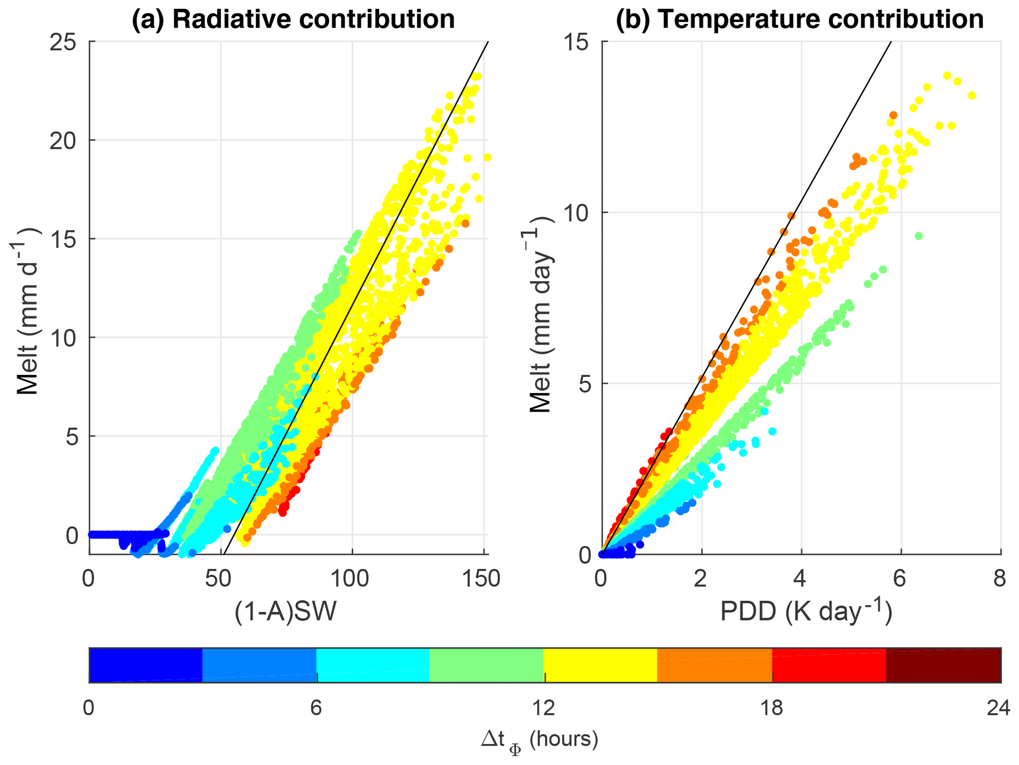
Figure 1 (a) Contribution of the first and third terms (radiative contribution) and (b) of the second term (temperature contribution) in Eq. (6) to monthly melt rates diagnosed with climatological temperatures and solar radiation from the MAR simulation. Colours indicate length of melt period (hours). The black lines represent the respective prediction of the dEBM_const according to Eq. (14).

Equations (6) and (14) appear formally similar, with the second term being temperature dependent (the temperature contribution) and the first and third term being independent of temperature and only dependent on solar radiation (the radiative contribution). However, the respective parameters cannot be compared directly, as Δt_Φ and q_Φ depend on latitude and month. Δt_Φ and q_Φ modulate the radiative contribution and Δt_Φ modulates the temperature contribution in Eq. (6). Figure 1a illustrates the radiative contributions and Fig. 1b the temperature contributions diagnosed from the MAR simulation in comparison to the respective contribution from the dEBM_const. On the GrIS the radiative contribution can exceed 25 mm day⁻¹ in the summer months and the two schemes appear qualitatively similar. The radiative contribution in the dEBM becomes less efficient for long melt periods, as the same insolation must balance the outgoing long-wave radiation for a longer time. On the other hand, the radiative contribution can also decrease towards short melt periods if the Sun only marginally rises above the minimum elevation angle at solar noon. At high latitudes, this effect becomes important for higher estimates of the minimum elevation angles (Sect. 4). The temperature contribution of the dEBM does not exceed 15 mm day⁻¹ (Fig. 1b) and becomes more efficient with longer melt periods and would agree with the dEBM_const for a melt period of 18 h.

Atmospheric forcing (insolation and temperature) and albedo are obtained here from the MAR output and are fully consistent with the MAR melt rates. Consequently, we can evaluate the skill of the considered schemes independently of the quality of the atmospheric forcing and the representation of albedo. On the other hand, we cannot evaluate the performance of the schemes for defective input. With respect to error propagation, the PDD scheme might be more robust, as it only requires temperature as a forcing and only distinguishes between snow and ice but does not require albedo. Given the ideal input, all schemes reproduce the year-to-year evolution of the total Greenland surface melt of the MAR simulation reasonably well (Fig. S3). The PDD scheme yields increasing errors with intensifying surface melt rates, which is not apparent for the dEBM_const and dEBM (Fig. 2). On the other hand, dEBM_const particularly overestimates (underestimates) melt rates for very short (long) melt periods. In comparison to the two empirical schemes, the dEBM produces smaller local errors with biases being pronounced only in a narrow band along the ice sheet's margins (Fig. 3).

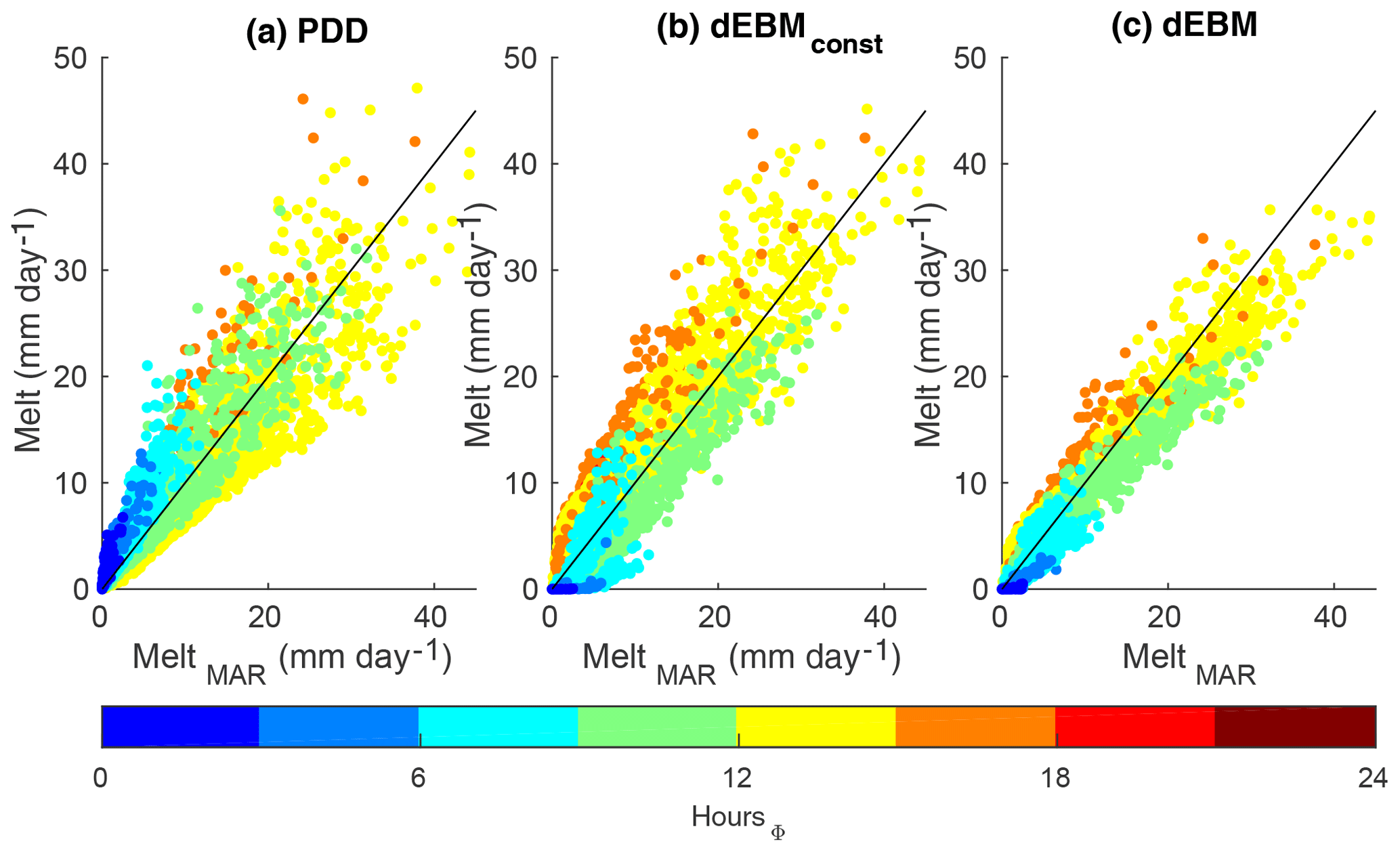
Figure 2 Multi-year monthly mean melt rates averaged over the years 1948–2016 and predicted by (a) the PDD scheme, (b) the dEBM_const and (c) the dEBM against respective MAR melt rates. Colours reflect the length of the daily melt period. Identity is displayed as a black line in all panels for comparison.

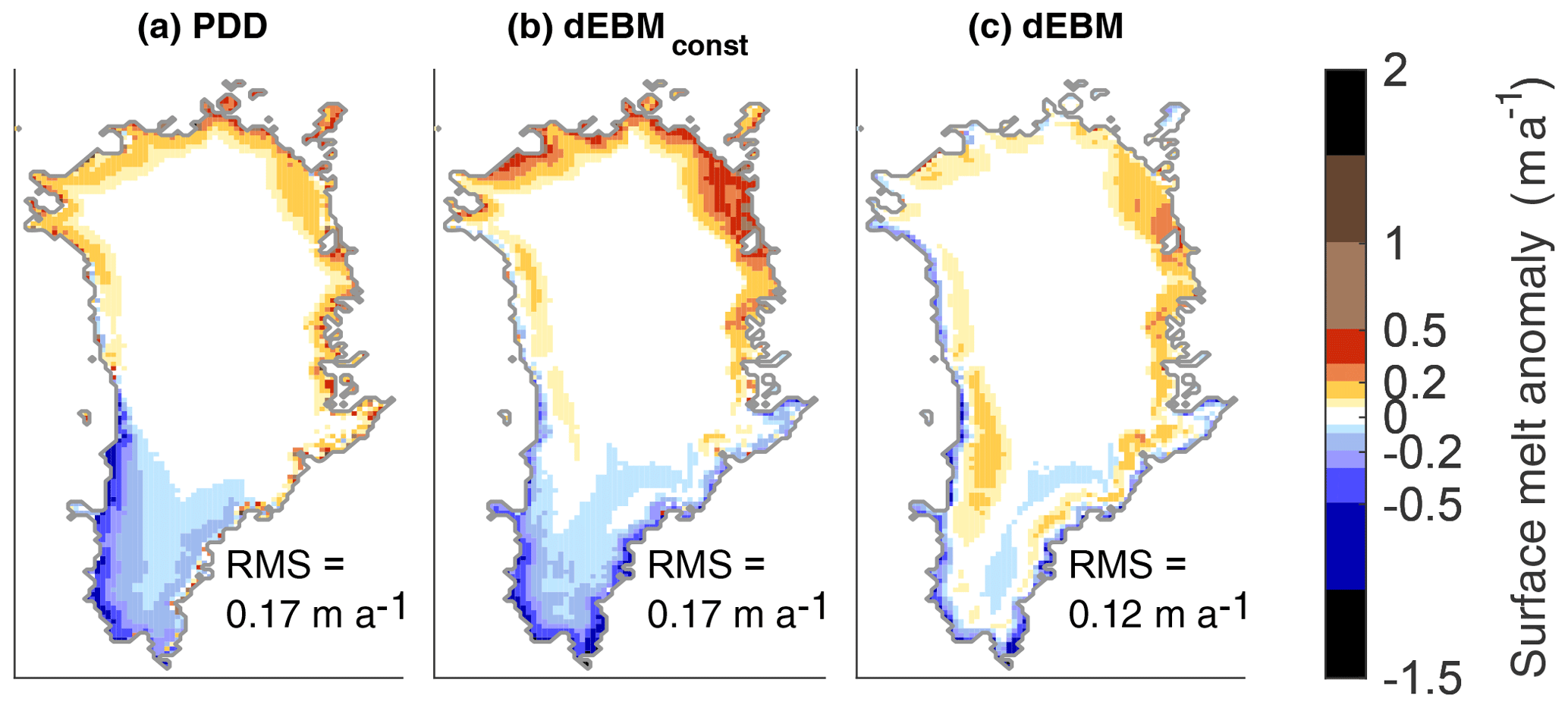
Figure 3 Bias between yearly melt rates predicted by the individual schemes and simulated by MAR, averaged over the whole simulation: (a) PDD, (b) dEBM_const and (c) the proposed new scheme dEBM. The respective root mean square error (RMSE) is given in the individual panels.

4 Sensitivity to model parameters and boundary conditions

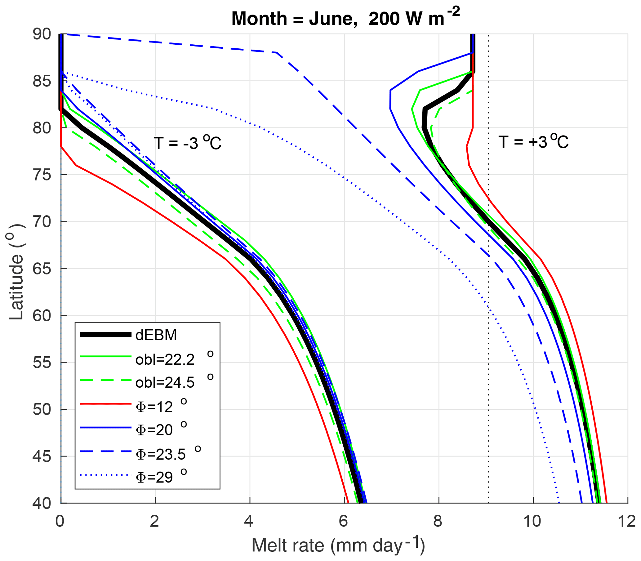
Figure 4 Sensitivity of the dEBM: June surface melt rate predicted for SW${}_{\mathrm{0}}=\mathrm{200}\mathrm{W}{\mathrm{m}}^{-\mathrm{2}}$, A=0.7, $T_{\mathrm{a}}=-\mathrm{3}$ ^∘C (left curves) and T_a=3 ^∘C (right curves). Black is predictions with parameters used for the presented simulation of Greenland's surface melt. Green is parameters recalculated using the minimum (solid) and maximum (dashed) obliquity of the last 1 million years. Blue is parameters recalculated for minimum elevation angles Φ of 20^∘ (solid), 23.5^∘ (dashed) and 29^∘ (dots) corresponding to a reduced solar density fluxes at the surface of $\mathit{\tau }{\widehat{S}}_{\mathrm{r}}=\mathrm{700}\mathrm{W}{\mathrm{m}}^{-\mathrm{2}}$, $\mathit{\tau }{\widehat{S}}_{\mathrm{r}}=\mathrm{600}\mathrm{W}{\mathrm{m}}^{-\mathrm{2}}$ and $\mathit{\tau }{\widehat{S}}_{\mathrm{r}}=\mathrm{500}\mathrm{W}{\mathrm{m}}^{-\mathrm{2}}$. Red is parameters recalculated for $\mathrm{\Phi }=\mathrm{12}{}^{\circ }$, which corresponds to an intensified solar density flux at the surface of $\mathit{\tau }{\widehat{S}}_{\mathrm{r}}=\mathrm{1150}\mathrm{W}{\mathrm{m}}^{-\mathrm{2}}$. The dEBM_const predicts 0 mm day⁻¹ for SW${}_{\mathrm{0}}=\mathrm{200}\mathrm{W}{\mathrm{m}}^{-\mathrm{2}}$, A=0.7, $T_{\mathrm{a}}=-\mathrm{3}$ ^∘C and 9 mm day⁻¹ for SW${}_{\mathrm{0}}=\mathrm{200}\mathrm{W}{\mathrm{m}}^{-\mathrm{2}}$, A=0.7, T_a=3 ^∘C (black dots).

4.1 Sensitivity to tuning parameters

In the above application, the parameters β for sensible heat and the background melting condition T_min have served as tuning parameters. The parameter $\mathit{\beta }=\mathrm{10}\mathrm{W}{\mathrm{m}}^{-\mathrm{2}}{\mathrm{K}}^{-\mathrm{1}}$ was determined by optimizing the scheme to MAR melt rates. This value agrees reasonably well with the moderate wind speeds found in PROMICE observations during melt periods (Fig. S2). Changing β by ±20 % changes the total annual Greenland surface melt by ±3 %. The choice of $T_{\min }=-\mathrm{6.5}$ ^∘C is in good agreement with observations, which reveal no substantial melt for temperatures $<-\mathrm{7}$ ^∘C (Orvig, 1954). Increasing the background melting condition T_min particularly reduces the melt rates at high elevations, while reducing T_min results in a longer melting season and increases the annual surface melt. Using no background melting condition at all, results in unrealistic melt rates at high elevations and would almost double the predicted total Greenland surface melt. Changing T_min by ±1 K changes the predicted mean annual surface melt by ±8 % for the MAR simulation used in this study. Intense surface melt is usually accompanied by warm temperatures and is thus insensitive to the choice of T_min. As refreezing particularly suppresses the contribution of weak surface melt at low temperatures, the resulting run-off can be expected to be less sensitive to the choice of T_min.

4.2 Sensitivity to diurnal cycle of solar radiation

Melt schemes which do not include the diurnal cycle of radiation will predict the same melt rate for a given combination of insolation and temperature forcing, irrespective of latitude or season. By contrast, Fig. 4 indicates a strong sensitivity in the dEBM surface melt predictions to latitude in summer. According to the dEBM, a short melt period with intensive solar radiation is causing melt more effectively than a longer melt period with accordingly weaker solar radiation. This sensitivity is particularly prominent in high latitudes and may explain the latitudinal bias found in many studies which do not resolve radiation on sub-daily timescales (Krapp et al., 2017; Krebs-Kanzow et al., 2018a; Plach et al., 2018).

4.3 Sensitivity to orbital configuration and transmissivity of the atmosphere

The TOA solar flux density $\widehat{S_{\mathrm{r}}}$ only depends on the distance between the Earth and Sun and due to the eccentricity of the Earth's orbit gradually varies by ±3.5 % from the solar constant from December to July respectively. On orbital timescales this seasonal deviation from the solar constant may amount to 10 %. Transmissivity τ and emissivity ϵ_a, on the other hand, strongly depend on cloud cover and atmospheric composition and additionally depend on the solar elevation angle. As a consequence, the minimum elevation angle Φ may be less then 13^∘ ($\mathit{\tau }\widehat{S_{\mathrm{r}}}=\mathrm{1150}\mathrm{W}{\mathrm{m}}^{-\mathrm{2}}$ for clear-sky, intense summer insolation). For overcast sky and weak summer insolation, we can ultimately expect $\mathit{\tau }\widehat{S_{\mathrm{r}}}<\mathrm{400}\mathrm{W}{\mathrm{m}}^{-\mathrm{2}}$. In that case, however, it is not justified to use the clear-sky emissivity in Eqs. (5) and (7). Consequently, the proposed scheme is no longer suitable, as net outgoing long-wave radiation will vanish and the energy balance will become very sensitive to turbulent heat fluxes. Applications aiming at continental ice sheets driven by climatological force will be restricted to a much narrower range of scenarios. As one can expect that transmissivity decreases towards the morning and afternoon hours, it may be justified to reduce the estimate of $\mathit{\tau }\widehat{S_{\mathrm{r}}}$ by a few percent. Figure 4 reveals that the scheme becomes very sensitive if the minimum elevation angle Φ takes values close to or larger than the obliquity of the Earth. Under such conditions, the duration of the melt period will vanish near the pole. However, the scheme is remarkably insensitive to intensified insolation (and accordingly reduced elevation angle Φ) or variations in the obliquity. Accordingly, estimating the elevation angle locally and for each month using Eq. (12), which is possible but computationally more expensive, does not noticeably improve the skill of the dEBM (not shown).

5 Discussion and conclusion

The presented new scheme for surface melt (dEBM) requires, like the insolation temperature melt scheme (ITM), monthly mean air temperatures and insolation as input but implicitly also includes the diurnal cycle. Together with suitable schemes for albedo and refreezing (Robinson et al., 2010), it may replace empirical surface melt schemes which are commonly used in ice sheet modelling on long timescales.

An application to the Greenland Ice Sheet indicates that the scheme may improve the spatial representation of surface melt in comparison to common empirical schemes. However, an evaluation against an independent data set is desirable. The most important advantage of the dEBM over empirical schemes may be that it can be globally applied to other ice sheets and glaciers and under different climate conditions, as parameters in the scheme are physically constrained and implicitly account for the orbital configuration.

In the presented formulation a threshold temperature serves as a prerequisite for surface melt on monthly timescales. This threshold temperature should be considered as a tuning parameter, as the representation of the ice–atmosphere boundary layer in Earth system models may differ considerably from the MAR simulation, which here has served as a reference. Furthermore, long-wave radiation and non-radiative heat fluxes are only crudely represented. Depending on the application, it may be advisable to adapt the parameterization of turbulent heat fluxes and long-wave radiation to different climate regimes in order to account for changed wind speed, humidity, cloud cover or greenhouse gas concentration.

The daily melt period is defined by a minimum solar elevation angle. Together with the melt period, parameters in the dEBM depend on latitude and month of the year but do not change from year to year if the minimum solar elevation angle is kept constant and the orbital configuration remains the same. For the Greenland Ice Sheet, a minimum solar elevation angle of 17.5^∘ was roughly estimated from the mean summer insolation normal to a surface at the bottom of the atmosphere. The dEBM is very sensitive if the intensity of solar radiation is substantially weaker than in the presented application (e.g. due to cloud cover or atmospheric water content). In this case it is necessary to carefully re-estimate the minimum elevation angle and to adjust the model parameters accordingly. Otherwise, the scheme appears to be relatively insensitive to changes in the orbital configuration and the parameters chosen in this study may be valid in a wider range of settings.

The presented formulation has been designed for long Earth System Model applications, but it may be adapted for use in the context of climate reconstructions or applied on regional or local scales. Furthermore, having defined the daily melt period by the minimum elevation angle, it should also be possible to estimate the amount of refreezing by considering the energy balance of the remainder of the day, following a similar approach to Krapp et al. (2017).