Ice cliff contribution to the tongue-wide ablation of Changri Nup Glacier, Nepal, central Himalaya

Ice cliff backwasting on debris-covered glaciers is recognized as an important mass-loss process that is potentially responsible for the “debris-cover anomaly”, i.e. the fact that debris-covered and debris-free glacier tongues appear to have similar thinning rates in the Himalaya. In this study, we quantify the total contribution of ice cliff backwasting to the net ablation of the tongue of Changri Nup Glacier, Nepal, between 2015 and 2017. Detailed backwasting and surface thinning rates were obtained from terrestrial photogrammetry collected in November 2015 and 2016, unmanned air vehicle (UAV) surveys conducted in November 2015, 2016 and 2017, and Pléiades tri-stereo imagery obtained in November 2015, 2016 and 2017. UAV- and Pléiades-derived ice cliff volume loss estimates were 3 % and 7 % less than the value calculated from the reference terrestrial photogrammetry. Ice cliffs cover between 7 % and 8 % of the total map view area of the Changri Nup tongue. Yet from November 2015 to November 2016 (November 2016 to November 2017), ice cliffs contributed to 23±5 % (24±5 %) of the total ablation observed on the tongue. Ice cliffs therefore have a net ablation rate 3.1±0.6 (3.0±0.6) times higher than the average glacier tongue surface. However, on Changri Nup Glacier, ice cliffs still cannot compensate for the reduction in ablation due to debris-cover. In addition to cliff enhancement, a combination of reduced ablation and lower emergence velocities could be responsible for the debris-cover anomaly on debris-covered tongues.

1 Introduction

Ablation areas in high-mountain Asia (HMA) are heavily debris-covered, meaning that a potentially large part of meltwater originates from ice ablation of debris-covered glacier tongues (Kraaijenbrink et al., 2017). Numerous studies have demonstrated that a debris layer thicker than 5–10 cm has a dominant insulating effect and dampens the ablation of ice beneath it (Lejeune et al., 2013; Nicholson and Benn, 2006; Reid and Brock, 2010; Reznichenko et al., 2010; Østrem, 1959). Yet counterintuitively, similar thinning rates (change in glacier surface elevation over time) have been observed for clean ice and debris-covered ice at similar elevations across HMA (Gardelle et al., 2013; Kääb et al., 2012). This debris-cover anomaly (Pellicciotti et al., 2015) has been observed in the Khumbu region (Nuimura et al., 2012), the Kangri Karpo Mountains (Wu et al., 2018) and at Kanchenjunga (Lamsal et al., 2017) and Siachen (Agarwal et al., 2017) glaciers.

Two main hypotheses have been proposed to explain this anomaly. First, while ablation rates are reduced by thick debris, ice cliffs act as local hotspots for melt and thus could contribute disproportionately to the tongue-averaged ablation (Buri et al., 2016a; Immerzeel et al., 2014; Pellicciotti et al., 2015; Reid and Brock, 2014; Sakai et al., 1998, 2002; Steiner et al., 2015). Additionally, other processes linked to supraglacial and englacial water systems could lead to substantial ablation (Benn et al., 2017; Miles et al., 2016, 2018; Sakai et al., 2000; Watson et al., 2018). Second, debris-covered tongues likely have a lower emergence velocity compared with debris-free tongues (Anderson and Anderson, 2016; Banerjee, 2017). As a result, similar thinning rates (surface mass-balance rate minus emergence velocity) could potentially be observed for debris-covered and clean ice glaciers, though the measured mass-balance rates would be more negative for clean ice.

In order to partially test the first hypothesis, there is a need to calculate the total contribution of the additional melt processes to the tongue-wide surface mass balance. In this work, we focus on the ice cliff contributions, as the processes related to the glacial water system are currently not quantifiable on the scale of a glacier tongue. For simplicity, hereafter we use the term “net ablation” instead of surface mass balance as we focus only on the ablation areas. We introduce the variable f_C, defined as the spatially integrated ratio between the net ablation from all ice cliffs and the net glacier tongue ablation, to quantify the enhanced ablation due to the presence of ice cliffs:

$$\begin{array}{}\text{(1)}& f_{\mathrm{C}}={\displaystyle \frac{{\dot{b}}_{\mathrm{C}}}{{\dot{b}}_{\mathrm{T}}}}={\displaystyle \frac{\mathrm{\Delta }{V}_{\mathrm{C}}}{A_{\mathrm{C}}}}\times {\displaystyle \frac{A_{\mathrm{T}}}{\mathrm{\Delta }{V}_{\mathrm{T}}}},\end{array}$$

where $\dot{b}$ is the net ablation, ΔV is the volume loss, A is the area, and the subscript refers to the cliffs (C) or the glacier tongue (T). Additionally, we define the quantity $f_{\mathrm{C}}^{\ast }$, which is the spatially integrated ratio between net ablation from all ice cliffs, and the net ablation on all non-cliff areas on the glacier tongue (denoted with the subscript NC):

$$\begin{array}{ll}{\displaystyle }{f}_{\mathrm{C}}^{\ast }& {\displaystyle }={\displaystyle \frac{{\dot{b}}_{\mathrm{C}}}{{\dot{b}}_{\mathrm{NC}}}}={\displaystyle \frac{\mathrm{\Delta }{V}_{\mathrm{C}}}{A_{\mathrm{C}}}}\times {\displaystyle \frac{A_{\mathrm{NC}}}{\mathrm{\Delta }{V}_{\mathrm{NC}}}}={\displaystyle \frac{\mathrm{\Delta }{V}_{\mathrm{C}}}{A_{\mathrm{C}}}}\times {\displaystyle \frac{A_{\mathrm{T}}-A_{\mathrm{C}}}{\mathrm{\Delta }{V}_{\mathrm{T}}-\mathrm{\Delta }{V}_{\mathrm{C}}}}\\ \text{(2)}& {\displaystyle }& {\displaystyle }=f_{\mathrm{C}}{\displaystyle \frac{\mathrm{\Delta }{V}_{\mathrm{T}}}{\mathrm{\Delta }{V}_{\mathrm{T}}-\mathrm{\Delta }{V}_{\mathrm{C}}}}{\displaystyle \frac{A_{\mathrm{T}}-A_{\mathrm{C}}}{A_{\mathrm{T}}}}.\end{array}$$

$f_{\mathrm{C}}^{\ast }$ has the advantage of not including the ice cliff contributions in the total tongue ablation, it is thus useful for modelling studies where sub-debris and cliff ablation are estimated independently or in order to scale the ice cliff ablation from the sub-debris ablation. f_C has the advantage of being directly linked to the total ice cliff contributions to ablation. $f_{\mathrm{C}}^{\ast }$ is expected to be larger than f_C, and both terms refer to a glacier-wide value.

Previous model-based estimates of f_C range between 6 and 14 (Buri et al., 2016b; Reid and Brock, 2014; Sakai et al., 2000), while values of $f_{\mathrm{C}}^{\ast }$ range between 7 (Juen et al., 2014) and 12 (Sakai et al., 2000). Two studies have quantified f_C using direct observations: Brun et al. (2016) found f_C=6 over Lirung Glacier by extrapolating volume losses measured from very high-resolution photogrammetry on a limited number of cliffs and Thompson et al. (2016) found a value of 8 by digital elevation model (DEM) differencing at Ngozumpa Glacier in the Nepalese Himalaya.

Emergence velocities (w_e) significantly greater than zero have been found previously on debris-covered glaciers, but w_e has been neglected in the calculation of f_C in all the above-mentioned studies. Values of w_e equal to 5.1–5.9±0.28 m a⁻¹ (Nuimura et al., 2011), 0.41 ± 0.05 m a⁻¹ (Vincent et al., 2016) and 0.00–0.35 ± 0.10 m a⁻¹ (Nuimura et al., 2017) have been found for, respectively, the debris-covered tongues of Khumbu, Changri Nup and Lirung glaciers in Nepal. However, we stress the fact that these emergence velocities have been measured at different locations of these debris-covered tongues (in particular close to the clean ice/debris transition on Khumbu Glacier) on glaciers with very different dynamics. Neglecting the emergence velocities (i.e. comparing thinning rates instead of ablation rates) introduces a systematic overestimation of f_C. This is due to the fact that cliffs ablate at higher rates than the rest of the glacier tongue: ice cliff thinning rates are thus less influenced than the thinning rates of debris-covered ice when neglecting the emergence velocity. As a consequence, the ratio of the cliff thinning rate divided by the mean tongue thinning rate will overestimate f_C. To correctly estimate f_C and the fraction of total ice cliff net ablation, thinning rates need to be corrected with the emergence velocity.

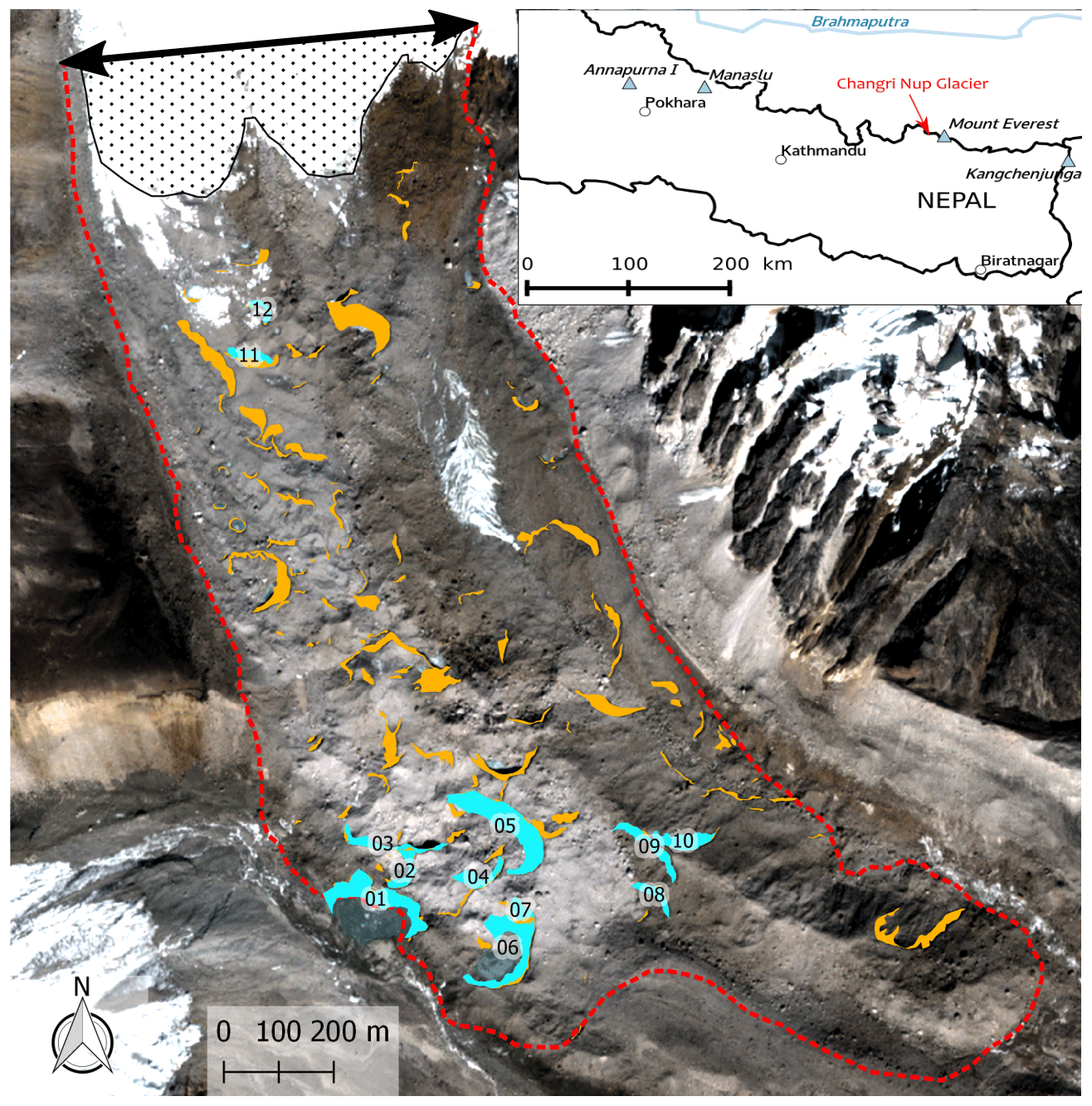
Figure 1 Map of Changri Nup Glacier tongue (red outline). The light-blue shapes are the 12 cliffs surveyed with the terrestrial photogrammetry and the orange shapes are all the cliffs of the tongue. The background image is the Pléiades images of November 2016 (copyright: CNES 2016, Distribution Airbus D&S). The ice thickness was measured along the black double-headed arrow in 2011 (Vincent et al., 2016). The dotted area is the debris-free part of the tongue (November 2017).

Recent studies advocate the use of terrestrial photogrammetry to understand patterns of ice cliff retreat (Watson et al., 2017). Nevertheless, these data can only be collected in the field with some difficulty and thus can only be acquired on a limited number of cliffs. Remote-sensing platforms (unmanned aerial vehicles, UAVs, or satellites) offer the potential to provide high-resolution topographic data with a glacier-wide or region-wide coverage but have not yet been evaluated for detailed multi-temporal monitoring of ice cliffs. Here we test the possibility to use gridded elevation data (i.e. DEMs) obtained from both UAV and Pléiades imagery to assess the total ice cliff contribution to the tongue-wide net ablation.

In this study, we use three very high-resolution topographic data sets based on terrestrial photogrammetry, UAV imagery and Pléiades imagery collected over the tongue of Changri Nup Glacier, Nepal between 2015 and 2017. From the terrestrial photogrammetry, 3-D models of 12 cliffs are created to calculate reference ice cliff volume losses from 2015 to 2016. We introduce a new method to calculate ice volume losses based on DEM differencing and geometric changes (e.g. ice emergence) induced by glacier flow. The new method is validated with terrestrial photogrammetric estimates of ice cliff volume loss and applied to the entire Changri Nup Glacier tongue to estimate the fraction of tongue-wide net ablation due to ice cliffs.

2 Study area

This study focuses on the debris-covered part of the tongue of Changri Nup Glacier, located in the Everest region of Nepal (Fig. 1). The glacier accumulates mass partly through avalanche deposition from the surrounding steep slopes (up to ∼6700 m a.s.l.) and flows down to 5250 m a.s.l. The local equilibrium line altitude (ELA) calculated for the nearby debris-free western Changri Nup Glacier is approximately 5600 m a.s.l. (Sherpa et al., 2017). We use the same glacier tongue outline as Vincent et al. (2016), which was derived from a combination of UAV imagery, velocities measured on the ground and field observations. This outline is substantially different from the outline available in the Randolph Glacier Inventory 6.0 (Pfeffer et al., 2014), which erroneously connects the debris-covered Changri Nup Glacier and the debris-free western Changri Nup Glacier.

Debris covers an area of 1.49±0.16 km² (Fig. 1) on the tongue of Changri Nup Glacier. Twelve ice cliffs were ground-surveyed (Table 1 and Fig. 1), and the analysis was then extended to more than 140 ice cliffs of various sizes (Fig. 1). The map view areas of all ice cliffs were $\mathrm{70}\pm \mathrm{14}\times {\mathrm{10}}^{\mathrm{3}}$, $\mathrm{72}\pm \mathrm{14}\times {\mathrm{10}}^{\mathrm{3}}$ and $\mathrm{70}\pm \mathrm{14}\times {\mathrm{10}}^{\mathrm{3}}$ m² in November of 2015, 2016 and 2017 (see Sect. 4.4.4 for the uncertainty assessment of the cliff map view areas).

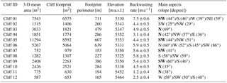
Table 1 Characteristics of the 12 surveyed cliffs. The 3-D mean area was calculated as the mean of the November 2015 and 2016 areas, which were measured from the PCs obtained with the terrestrial photogrammetry on CloudCompare. The perimeter was calculated from the cliff footprint of November 2015 and 2016. The backwasting rate was calculated as the ratio between the cliff backwasting volume obtained from terrestrial photogrammetry and the 3-D mean area, for the period November 2015–November 2016. The cliffs are usually not perfectly planar and they exhibit multiple aspects. The main aspects were calculated by fitting a plan through the cliff PC or through parts of the PC in CloudCompare. The main aspect is in bold when it was possible to determine it.

3 Data

3.1 Terrestrial photogrammetry

Terrestrial photographs of 12 ice cliffs (Table 1) were collected during two field campaigns: 24–28 November 2015 and 9–12 November 2016, using survey methods similar to those described in Brun et al. (2016) and Watson et al. (2017). Between 200 and 400 photographs of each ice cliff were taken from various camera positions using a Canon EOS5D Mark II digital reflex camera with a Canon 50 mm f/2.8 fixed focal length lens (Vincent et al., 2016). For each ice cliff, we derived point clouds (PCs) and triangulated irregular networks (TINs) with Agisoft Photoscan 1.3.4 Professional (Agisoft, 2017). In order to align the photographs and georeference the final point clouds and derived products, between 7 and 17 ground control points (GCPs) made of pink fabric were spread around each cliff. GCP positions were surveyed with a Topcon differential global positioning system (DGPS) unit with a precision of ∼0.10 m. All markers were used as GCPs and therefore no independent markers were available for validation. After optimization of the photographs' alignment, the marker residuals were on average 0.27 m for the 2015 campaign and 0.18 m for the 2016 campaign. The 3-D area of the surveyed cliffs ranged from 600 m² to more than 11 000 m² (Table 1).

3.2 UAV photogrammetry

UAV imagery of Changri Nup Glacier was obtained in November of 2015, 2016 and 2017 using the Sony Cyber-shot WX DSC-WX220 mounted on the fixed-wing eBee UAV manufactured by senseFly (Table 2). Aerial imagery was processed using a structure from motion (SfM) procedure in Agisoft Photoscan (see Vincent et al., 2016 and Kraaijenbrink et al., 2016 for details) to produce dense point clouds. Orthomosaics (0.10 m resolution) and DEMs (0.20 m resolution) were produced for each year. An additional mission and processing details for each year are given below.

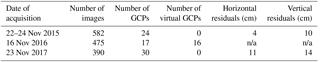
Table 2 Characteristics of the three UAV flights. The horizontal and vertical residuals are assessed on independent additional GCPs. The virtual GCPs are reference points taken in stable ground from the 2015 UAV DEM and orthomosaic, and used as GCPs to derive the 2016 UAV DEM and orthomosaic. For the 2015 and 2017 campaigns, the GCPs were in sufficient number and consequently we did not use virtual GCPs. For the 2016 campaign, we used all the available GCPs to derive the DEM, and consequently could not evaluate the residuals.

n/a – not applicable

In 2015, five separate eBee flights between 22 and 24 November were flown to cover the surface of the glacier. The data were georeferenced using a set of 24 GCPs that were spatially well distributed and measured using the Topcon DGPS (Fig. S1 in the Supplement). Based on 10 additional independent GCPs, the error of the 2015 UAV product was determined to be 0.04 m horizontally and 0.10 m vertically, which is in the range of expected accuracy (Gindraux et al., 2017).

On 10 November 2016, Changri Nup was surveyed with three eBee flights. To georeference the 2016 UAV imagery, we distributed a total of 17 markers on the glacier and measured their coordinates with the Topcon DGPS. Unfortunately, due to time constraints, the resulting spatial distribution of the markers was suboptimal (Fig. S1). Using only these markers as GCPs had considerable consequences for processing accuracy, and we therefore defined 16 additional virtual tie points. Tie point coordinates were sampled from the November 2015 UAV orthomosaic and DEM (Fig. S1), and we selected specific features on boulders that were (a) clearly identifiable on both the 2015 and 2016 image sets and (b) located on stable terrain (Immerzeel et al., 2014), which we determined from visual inspection of the Pléiades orthoimages and DEMs.

In 2017, three separate flights were used to survey the glacier on 23 November, and 30 GCPs were collected (Fig. S1). Residuals, based on six independent check points, were 0.10 m horizontally and 0.14 m vertically.

3.3 Pléiades tri-stereo photogrammetry

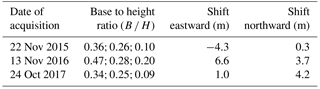
Three triplets of Pléiades images were acquired over the study area on 22 November 2015, 13 November 2016 and 24 October 2017 (Table 3). The along-track angles of the acquisitions gave base-to-height ratios that ensured suitable stereo capabilities (Belart et al., 2017). For each acquisition, we derived a 2 m DEM and a 0.5 m orthoimage using the Ames Stereo Pipeline (Shean et al., 2016) using only the rational polynomial coefficients (RPCs) provided with the imagery (no GCPs) and the same processing parameters as Marti et al. (2016). We used the stereo routine of ASP to derive one PC from each triplet of images, which was gridded into a single 2 m DEM using the point2dem routine. Orthoimages were generated from the image closest to the nadir using the mapproject function and a 2 m resolution DEM, which was gap filled with 4 and 8 m DEM resolutions derived similarly. This ensured sharp and gap-free images.

Each Pléiades orthoimage was co-registered to the corresponding UAV orthomosaic by visually matching boulders on stable ground. The accuracy of this co-registration was examined by calculating the median displacement on a 2.4 km² area of stable terrain located off-glacier. An east-to-west residual displacement of 0.05 m and a north-to-south residual displacement of −0.09 m was identified after co-registration. This absolute co-registration was needed to compare the UAV and Pléiades data sets, but would not be necessary while working with Pléiades data only. In the latter case, the robustness of the Pléiades processing based only on RPCs would be sufficient to co-register the images and DEMs relatively using automatic co-registration methods.

Each Pléiades DEM was shifted with the same horizontal displacement as the corresponding orthoimage (Table 3). Automatic co-registration methods applied to the manually shifted DEMs (Berthier et al., 2007; Nuth and Kääb, 2011) resulted in no improvement of the standard deviation of elevation changes on stable terrain. Thus, no further horizontal shift was applied. The vertical shift between the two Pléiades DEMs, calculated as the median elevation change on stable terrain, was equal to −7.43 and −3.31 m for the periods November 2015–November 2016 and November 2016–November 2017. These vertical offsets are quite large but expected, as the DEMs are derived from the orbital parameters only (Berthier et al., 2014). We corrected these offsets by subtracting them from the elevation difference map. Elevation changes over stable terrain have no relation to the slope, aspect or curvature (Fig. S2).

For these three satellite-based data sets, the duration between acquisition dates was 350 to 381 days. All displacements and volumes were linearly adjusted (divided by the number of days between the acquisition dates and multiplying by the total number of days in a year) to obtain annual velocities and volume change rates.

3.4 Update of existing data sets

We updated two data sets from Vincent et al. (2016): the glacier surface velocity and the cross-sectional ice thickness data.

3.4.1 Surface velocity fields

Surface velocity fields were derived from the correlation of the Pléiades orthoimages and UAV orthomosaics using COSI-corr (Leprince et al., 2007). The UAV orthomosaics were resampled to a resolution of 0.5 m to match the Pléiades orthoimages. For both data sets we chose an initial correlation window size of 256 pixels and a final size of 16 pixels (Kraaijenbrink et al., 2016). The step was set to 16 pixels, leading to a final grid spacing of 8 m.

Table 3 Characteristics and IDs of the Pléiades images. Horizontal shifts relative to the UAV orthoimages are also given. Each base-to-height ratio corresponds to a stereo pair.

The raw correlation outputs were filtered to retain pixels with a signal to noise ratio larger than 0.9. We manually removed pixels at ice cliff locations, as cliff retreat led to large geometric changes and therefore poor correlation. These outputs were filtered with a 9×9 pixel window moving median filter and then gap filled with a bilinear interpolation (Fig. 2). The patterns of displacement from UAV and Pléiades are in very good agreement. The velocities measured with Pléiades match well with the field data (ablation stake displacements measured with a DGPS between November 2015 and November 2016), with the notable exception of a stake located where the velocity gradient is high and for which the Pléiades images could not be correlated due to snow, leading to a poor bilinear interpolation (Fig. S3). Nevertheless, the maximum displacement in the remote sensing data (around 11 m a⁻¹) is less than that observed in the 2011–2015 field data (Vincent et al., 2016). This is due to a slow-down of the glacier that is also observed in the 2015–2016 field data.

Figure 2 Annual horizontal velocity fields deduced from the correlation of Pléiades orthoimages. Coordinates are in UTM 45/WGS 84. The black line is the tongue outline. The missing data in the velocity fields were filled using linear interpolation.

3.4.2 Cross section of ice thickness

A cross-sectional profile of ice thickness was measured upstream of the debris-covered tongue (Fig. 1) in October 2011, with a ground-penetrating radar (GPR) working at a frequency of 4.2 MHz (Vincent et al., 2016). The original cross-sectional area was 79 300 m² in 2011 and 78 200 m² in 2015 (Vincent et al., 2016). Between November 2015–November 2016 and November 2016–November 2017, the cross-sectional area decreased from S_2015–2016=76 900 m² to S_2016–2017=76 340 m² (with S_yr1−yr2 being the mean cross-sectional area between the year 1 and 2), based on the 0.86 m a⁻¹ thinning rate measured over the November 2015–November 2017 period along the profile. Following Azam et al. (2012), who measured the ice thickness of Chhota Shigri Glacier (15.48 km² flowing from 5830 to 4050 m a.s.l. with a maximum measured ice thickness of ∼270 m) using the same methods, we estimated that the absolute uncertainty in the ice thickness is ±15 m, which leads to an uncertainty in the cross-sectional area (σ_S) of ±10 000 m², as the length of the cross section is 670 m.

4 Methods

4.1 Emergence velocity

The emergence velocity refers to the upward flux of ice relative to the glacier surface in an Eulerian reference system (Cuffey and Paterson, 2010). For the case of a glacier in steady state (i.e. no volume change on the annual scale), the emergence velocity balances the net ablation for any point of the glacier ablation area exactly (Hooke, 2005). For a glacier out of its steady state (such as Changri Nup Glacier) the thinning rate in the ablation area is the sum of the net ablation and the emergence velocity (Hooke, 2005). On debris-covered glaciers, while the thinning rate is relatively straightforward to measure from DEM differences, for example, the ablation is highly variable in space and difficult to measure (Vincent et al., 2016). In order to evaluate the mean net ablation of Changri Nup Glacier tongue from the thinning rate, we estimate mean emergence velocities (w_e) for November 2015–November 2016 and November 2016–November 2017 using the flux gate method of Vincent et al. (2016). As the ice flux at the glacier front is 0, the average emergence velocity downstream of a cross section can be calculated as the ratio of the ice flux through the cross section (Φ in m³ a⁻¹), divided by the glacier area downstream of this cross section (A_T in m²):

$$\begin{array}{}\text{(3)}& w_{\mathrm{e}}={\displaystyle \frac{\mathrm{\Phi }}{A_{\mathrm{T}}}}.\end{array}$$

This method requires an estimate of ice flux through a cross section of the glacier and is based here on measurements of ice depth and surface velocity along a profile upstream of the debris-covered tongue (Figs. 1 and 2). The ice flux is the product of the depth-averaged velocity ($\overline{u}$ in m a⁻¹) and the cross-sectional area. For the periods November 2015–2016 and November 2016–2017, centerline velocities were equal to 10.8 and 11.1 m a⁻¹. Assuming that mean surface velocity is usually 70 % to 80 % of the centerline velocity (Azam et al., 2012; Berthier and Vincent, 2012) gives mean surface velocities along the upstream profile of 8.1±0.6 m a⁻¹ in 2015–2016, and 8.3±0.6 m a⁻¹ for 2016–2017. We used the relationship between the centerline velocity and the mean velocity, instead of an average of the velocity field along the cross section, because the image correlation was not successful on a relatively large fraction (∼30 %) of the cross section.

Converting the surface velocity into a depth-averaged velocity requires assumptions about basal sliding and a flow law (Cuffey and Paterson, 2010). Little is known about the basal conditions of Changri Nup Glacier, but Vincent et al. (2016) assumed a cold base and therefore no sliding. This leads to $\overline{u}$ being approximated as 80 % of the surface velocity, assuming n=3 in Glen's flow law (Cuffey and Paterson, 2010). As an end-member case, assuming that the motion is entirely by slip implies $\overline{u}$ equals the surface velocity (Cuffey and Paterson, 2010). Consequently, we followed Vincent et al. (2016) and assumed no basal sliding, but we took the difference between the two above-mentioned cases as the uncertainty in $\overline{u}$. This gives $\overline{u}=\mathrm{6.5}\pm \mathrm{1.6}$ m a⁻¹ for 2015–2016 and $\overline{u}=\mathrm{6.6}\pm \mathrm{1.7}$ m a⁻¹ for 2016–2017.

Assuming that the uncertainty related to the cross-sectional area (σ_S) and the uncertainty related to depth-averaged velocity (${\mathit{\sigma }}_{\overline{u}}$) are independent, uncertainty in the ice flux (σ_Φ) can be estimated as follows:

$$\begin{array}{}\text{(4)}& {\displaystyle \frac{{\mathit{\sigma }}_{\mathrm{\Phi }}}{\mathrm{\Phi }}}=\sqrt{({\displaystyle \frac{{\mathit{\sigma }}_{\overline{u}}}{\overline{u}}}{)}^{\mathrm{2}}+({\displaystyle \frac{{\mathit{\sigma }}_{\mathrm{S}}}{S}}{)}^{\mathrm{2}}}.\end{array}$$

Given the above-mentioned values for the depth-averaged velocity, the cross-sectional area and the associated uncertainties, the relative uncertainty in the estimated ice flux is ∼30 %. As a result, for the November 2015–2016 and November 2016–2017 periods, the ice fluxes were 499 700±150 000 and 503 840±150 000 m³ a⁻¹. The glacier tongue area was considered unchanged at 1.49±0.16 km², corresponding to $w_{\mathrm{e}}=\mathrm{0.33}\pm \mathrm{0.11}$ m a⁻¹ for 2015–2016 and $w_{\mathrm{e}}=\mathrm{0.34}\pm \mathrm{0.11}$ m a⁻¹ for 2016–2017.

It is notoriously difficult to delineate debris-covered glacier tongues (Frey et al., 2012). Uncertainty in the outline position of ±20 m leads to a relative uncertainty in the glacier area of 11 %, which is higher than the 5 % given by Paul et al. (2013). In this case, the uncertainty in the glacier outline is not the main source of uncertainty in w_e. However, if we had used automatically delineated outlines, this would be an important source of uncertainty. The updated emergence velocity is ∼20 % lower than estimated for the 2011-2015 period (Vincent et al., 2016) due to both the thinning and deceleration of the glacier at the cross section. As the difference in w_e between November 2015–November 2016 and November 2016–November 2017 is insignificant, we consider w_e to be constant and equal to $w_{\mathrm{e}}=\mathrm{0.33}\pm \mathrm{0.11}$ m a⁻¹ for the rest of this study. It is noteworthy that w_e is likely to be spatially variable. However, we have no means to assess its spatial variability.

4.2 Ice cliff backwasting calculation

4.2.1 Point cloud deformation

Every point on the glacier surface moves with a horizontal velocity u_s along a surface slope α and is advected upwards following the vertical velocity w_s (Cuffey and Paterson, 2010; Hooke, 2005):

$$\begin{array}{}\text{(5)}& w_{\mathrm{s}}=u_{\mathrm{s}}\tan \mathit{\alpha }+w_{\mathrm{e}}.\end{array}$$

When DEM differencing is applied, observed thinning rates at every point on the glacier surface is a combination of net ablation and displacement caused by glacier flow. In order to exclusively measure the volume loss associated with the net ablation, we deformed the PCs by displacing individual points for the data sets acquired in November 2015 and in November 2016. This accounts for three-dimensional glacier flow between November 2015 and November 2016 and between November 2016 and November 2017, respectively. For the terrestrial photogrammetry and UAV data, we applied these deformations directly to each point in the PCs. For the Pléiades data, we artificially oversampled the DEM on a 0.5 m resolution grid and converted this DEM to a PC, using the gdal_translate function. All the points of the PCs were displaced in x, y and z direction:

$$\begin{array}{}\text{(6)}& \left\{\begin{array}{l}{x}_{t+\mathrm{d}t}=x_t+u_{\mathrm{s},x}\mathrm{d}t\\ y_{t+\mathrm{d}t}=y_t+u_{\mathrm{s},y}\mathrm{d}t\\ z_{t+\mathrm{d}t}=z_t+w_{\mathrm{s}}\mathrm{d}t\end{array},\right.\end{array}$$

where u_s,x and u_s,y are the x and y components of the horizontal velocity, dt is the duration between the two acquisitions and z is the glacier surface elevation.

Figure 3 Definition of the different flow components, u_s is the horizontal velocity, w_s the vertical velocity and α the angle of the glacier surface tangent; adapted from Hooke (2005).

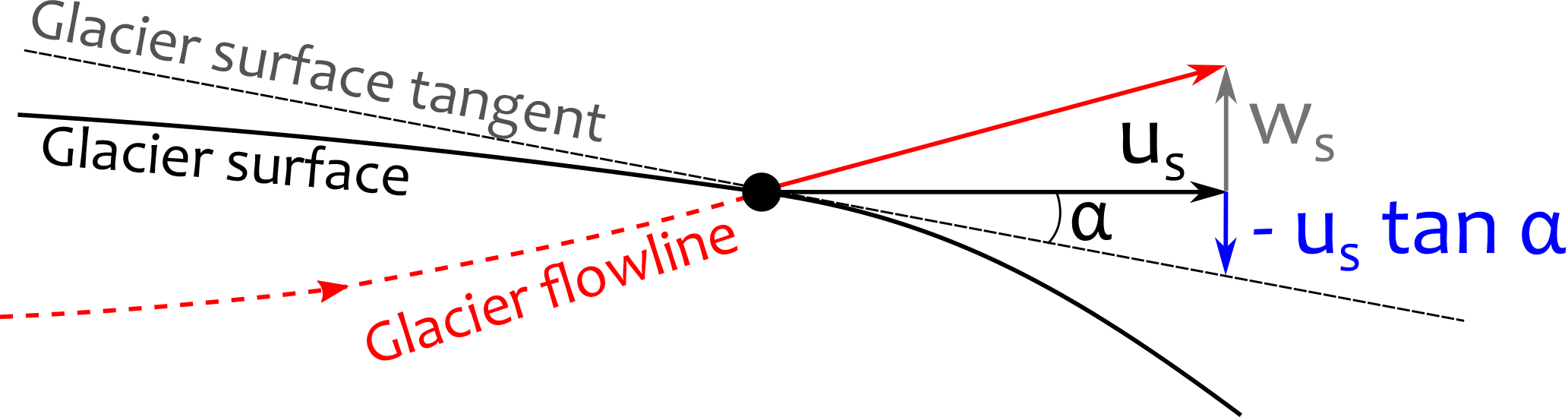
Even though w_e is likely to be spatially variable, we consider it to be homogeneous over the whole ablation tongue. The horizontal velocity u_s was directly taken from the bilinear interpolation of the Pléiades velocity field (Fig. 2). The term u_stanα, can be expressed as follows:

$$\begin{array}{}\text{(7)}& u_{\mathrm{s}}\tan \mathit{\alpha }={\displaystyle \frac{z(x+u_{\mathrm{s},x}\mathrm{d}t,y+u_{\mathrm{s},y}\mathrm{d}t)-z(x,y)}{\mathrm{d}t}}.\end{array}$$

As the ice flows along the longitudinal gradient instead of the rough local surface slope, we extracted z from a version of the Shuttle Radar Topography Mission (SRTM) DEM smoothed with a Gaussian filter using a 30 pixel kernel size (Fig. S4).

For the Pléiades and UAV data, we then gridded the deformed PCs using the point2dem ASP function (Shean et al., 2016) and derived the associated maps of elevation changes (Figs. 4 and 5).

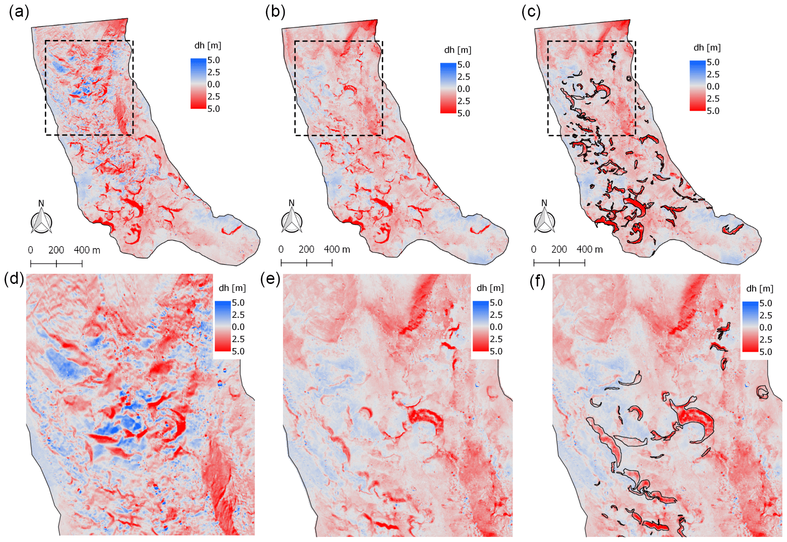
Figure 4 Panels showing maps of elevation change from UAV (a, d) before flow correction and (b, c, e, f) after flow correction over the period 23 November 2015–16 November 2016. Black outlines on panels (c) and (f) are the cliff footprints. Panels (d), (e) and (f) are close-ups of the panels (a), (b) and (c).

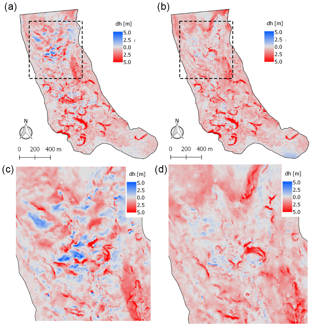
Figure 5 Panels showing maps of elevation change from Pléiades (a, c) before flow correction and (b, d) after flow correction over the period 22 November 2015–13 November 2016. Panels (c) and (d) are close-ups of the panels (a) and (b).

4.2.2 Ice cliff volume change from TINs

In order to measure the volume changes due to cliff retreat from the TINs derived from terrestrial photos, we applied the method from Brun et al. (2016) with some methodological improvements. First, the field of displacement was assumed to be homogeneous on the cliff scale in Brun et al. (2016). In this study, we use interpolated values of the local field of displacement with a resolution of 8 m. This would be an important methodological refinement for ice cliffs on fast-flowing glaciers with a rotational component, but has a minor influence on the cliffs of interest in this study (Fig. S5a). Second, we added more analogous points in the cliff edge triangulation method. Analogous points are points that are assumed to match in the two acquisitions (e.g. the corners of cliffs; Fig. S5b). Brun et al. (2016) discretized the triangulation problem assuming that the final number of points were equal on the upper and on the lower side of the cliff outline (i.e. implicitly assuming that the two corners of the cliffs were the only analogous points). In this study, the operator can choose how many analogous points are needed to link the two cliff outlines. Consequently, the method is now able to handle larger geometry changes than previously, under the assumption that some analogous parts of the cliffs are identifiable on both cliff outlines.

4.2.3 Ice cliff volume change from DEMs

To calculate ice cliff volume change from the DEMs, the mean elevation change was corrected for glacier flow below a cliff mask multiplied by the projected map view area of the mask. The cliff mask was defined as the union of the shapefiles of the cliff outlines and is called the cliff footprint and denoted A_2−D hereafter. The cliff outlines were manually delineated both on the Pléiades and UAV orthoimages for November 2015, November 2016 and November 2017. For each acquisition, we used deformed outlines of November  2015 and November 2016 cliffs when working with the corresponding deformed DEM difference. We manually edited the cliff mask to make sure we included the terrain along which the cliff retreated. In particular, this implied linking the corners of the cliff outlines of the two acquisitions in many cases (Fig. S5c).

4.3 Sources of uncertainty in the ice cliff backwasting

The main sources of uncertainties on the volume loss estimates are (1) the uncertainty in the spatial distribution of the emergence velocity (σ_e); (2) uncertainties of the horizontal surface displacement (σ_d); (3) uncertainty introduced by the displacement along the slope (σ_w); (4) uncertainties of the cliff outline delineation (σ_m) and (5) uncertainties of the various representations of the glacier surface in TINs and DEMs (σ_z). The first, second and third sources of uncertainties are common to the three data sets and the third and fourth ones are specific to each data set. We assume these five sources of uncertainty to be independent.

4.3.1 Emergence velocity

We calculated a mean emergence velocity for the tongue of 0.33±0.11 m a⁻¹, but as the spatial variability was unknown extreme values of emergence velocities were tested to estimate σ_e. We choose 0.00 m a⁻¹ as a lower limit because the emergence velocity is positive in the ablation area (Cuffey and Paterson, 2010; Hooke, 2005). For a thinning glacier, the net ablation is higher than the emergence velocity (Hooke, 2005). Consequently, the net ablation can be used as a proxy for the upper bound for the emergence velocity. The maximum net ablation measured with stakes within the period 2014–2016 on the tongue of Changri Nup (2.22 m a⁻¹) was chosen as the upper limit (Vincent et al., 2016). We tested these values on the terrestrial photogrammetry-based volume change estimate of each cliff (Fig. 6a). Except for cliff 11, the relative volume change that resulted from the test was always below +40 % for an increase in the emergence velocity and −5 % for a decrease in the emergence velocity. Cliff 11 likely exhibits a high sensitivity to the emergence velocity due to its relatively shallow slope and its very small volume loss (Tables 1 and S1 in the Supplement). The tested range of values of emergence velocities is rather extreme for the case of Changri Nup Glacier, and we therefore assumed that the uncertainty due to the emergence velocity was equal to the median of the relative volume change for an increase in the emergence velocity (23 %). As a consequence, σ_e=0.23 V, where V is the cliff volume change.

Figure 6 Sensitivity of the volume change estimate to the emergence velocity for each cliff with two tested emergence velocities (a) and for all cliffs with various emergence velocities tested (b). The relative volume change is the tested volume change minus the reference volume change (obtained for w_e=0.33 m a⁻¹), divided by the reference volume change and multiplied by 100. In the lower panel, each cross represents a cliff and the open circles represent the median; note that relative volume changes of cliff 11 are not visible for emergence velocities of 3.0 and 5.0 m a⁻¹, because they are equal to 153 % and 255 %. The volume estimates are from terrestrial photogrammetry data for the period November 2015–November 2016.

4.3.2 Horizontal displacement

The quality of the horizontal surface displacement derived from Pléiades orthoimages was evaluated by comparison with field measurements of the surface displacement. The median of the absolute difference between the 16 field measurements (stakes and marked rocks) and the corresponding Pléiades measurements was 30.8 cm. We therefore assumed that the uncertainty introduced by the horizontal displacement (σ_d) is 30 cm. The conversion into volumetric uncertainty, σ_d, was made by multiplying this uncertainty by the 3-D cliff area (A_3-D) for the terrestrial photogrammetry and by the cliff footprint area (A_2-D) for the UAV and Pléiades (Table 1).

4.3.3 Displacement along the glacier slope

The uncertainty in u_stanα depends mostly on the uncertainty in the mean slope of the surrounding glacierized surface (Hooke, 2005). Kernel sizes of 5 and 60 pixels used to filter the SRTM DEM produced respective mean elevation changes on the cliff mask of −0.51 and −0.33 m a⁻¹. As these values correspond to relatively sharp and very smooth DEMs, half of the difference between these two values (10 cm) is a good proxy for the uncertainty due to this correction. We converted this uncertainty into a volumetric uncertainty (σ_w) by multiplying it by the cliff 3-D area (A_3-D) for the terrestrial photogrammetry and by the cliff footprint area (A_2-D) for the UAV and Pléiades.

4.3.4 Cliff mapping

The uncertainty in the cliff mapping from Pléiades orthoimages was empirically assessed by asking eight different operators (most of the co-authors of this study) to map six cliffs for which we had reference outlines from the terrestrial photogrammetry. The operators had access to the Pléiades orthoimage of November 2016 and to the corresponding slope map. We calculated a normalized length difference defined as the difference between the area mapped by the operator and the reference area divided by the outline perimeter. The median normalized length difference ranged between −0.7 and 1.7 m and was on average equal to 0.6 m, meaning that the operators systematically overestimated the cliff area. The mean of the absolute value of the median normalized length difference was 0.8 m, which was used as an estimate for the cliff area delineation uncertainty. We conservatively assumed the same value for the Pléiades orthoimages and UAV orthomosaics, even though it should be lower for the UAV orthomosaics because of their higher resolution. For the terrestrial photogrammetry data, we assumed no uncertainty in the cliff area. The volumetric uncertainty σ_m was obtained by multiplying this value by the perimeter of cliff footprint and by the mean elevation change from DEM differences for UAV and Pléiades.

4.3.5 Accuracy of the topographic data

The uncertainty in the vertical accuracy of the terrestrial photogrammetry was directly estimated as the mean of the GCP residual of all cliffs (0.21 m). For the UAV and Pléiades orthoimages we followed the classical assumption of partially correlated errors (Fischer et al., 2015; Rolstad et al., 2009) and therefore σ_z is given by the following:

$$\begin{array}{}\text{(8)}& {\mathit{\sigma }}_{\mathrm{z}}=\left\{\begin{array}{ll}{A}_{\text{2-D}}{\mathit{\sigma }}_{\mathrm{\Delta }h}\sqrt{{\displaystyle \frac{A_{\mathrm{cor}}}{\mathrm{5}{A}_{\text{2-D}}}}}& ;A_{\text{2-D}}\ge A_{\mathrm{cor}}\\ A_{\text{2-D}}{\mathit{\sigma }}_{\mathrm{\Delta }h}& ;A_{\text{2-D}}<A_{\mathrm{cor}}\end{array},\right.\end{array}$$

where A_cor=πL², with L being the decorrelation length and σ_Δh being the normalized median of absolute difference (Höhle and Höhle, 2009) of the elevation difference on stable ground. We experimentally determined L=150 m for both the UAV and Pléiades data, even though the spherical model did not fit the Pléiades semi-variogram very well. We found σ_Δh=0.27 m for the UAV and 0.36 m for Pléiades.

Under the assumption that the different sources of uncertainty are independent, the final uncertainty in the volume estimate σ_V is as follows:

$$\begin{array}{}\text{(9)}& {\mathit{\sigma }}_V=\sqrt{{\mathit{\sigma }}_{\mathrm{e}}^{\mathrm{2}}+{\mathit{\sigma }}_{\mathrm{d}}^{\mathrm{2}}+{\mathit{\sigma }}_{\mathrm{w}}^{\mathrm{2}}+{\mathit{\sigma }}_{\mathrm{m}}^{\mathrm{2}}+{\mathit{\sigma }}_{\mathrm{z}}^{\mathrm{2}}}.\end{array}$$

5 Results

5.1 Comparison of TIN-based and DEM-based estimates

The volume changes estimated from terrestrial photogrammetry (our reference) and from UAV and Pléiades data are in good agreement and within error bars (Table S2 and Fig. 7). The total volume loss estimates for these 12 cliffs for the period November 2015–November 2016 are 193 453±19 647 m³ a⁻¹ using terrestrial photogrammetry and 188 270±20 417 and 181 744±19 436 m³ a⁻¹ using UAV and Pléiades. The total relative difference is therefore −3 % for the UAV and −7 % for Pléiades, which is smaller than the uncertainty in each estimate (∼10 %, calculated as the quadratic sum of the 12 individual cliff uncertainty estimates, assumed to be independent). The total Pléiades and UAV estimates are lower than the reference estimate; nevertheless, this is probably due to the estimate of the largest cliff (cliff 01), as there is no systematic underestimation of the volume for individual cliffs (Fig. 7).

Figure 7 Comparison of the ice cliff volume changes estimated from DEM differences between Pléiades (a) or UAV (b) and terrestrial photogrammetry for the period November 2015–November 2016. Note the log-scale. For each panel, “corrected” means taking into account the geometric corrections due to glacier flow and “non-corrected” means neglecting them.

5.2 Sensitivity to the emergence velocity

As Changri Nup Glacier is a slow-flowing glacier, the emergence velocity is small and the associated uncertainty is low (Fig. 6a). Nevertheless, with our data set it is possible to explore more extreme emergence velocities up to 5 m a⁻¹, which is a value inferred for a part of the Khumbu Glacier tongue and which is also the maximum emergence velocity measured on a debris-covered tongue (Nuimura et al., 2011). Our results show that, as a rule of thumb, every 1 m a⁻¹ error on the emergence velocity would increase the 1-year volume change estimate by 10 % (Fig. 6b). It is noteworthy that the main source of uncertainty in the cliff volume change is the uncertainty in the emergence velocity.

5.3 Importance of the glacier-flow corrections

In order to check the internal consistency of the glacier-flow correction, we calculated mean net ablation over the glacier tongue (the mean rate of elevation change minus the emergence velocity) before and after corrections. For the period November 2015–November 2016, without flow correction the mean tongue net ablation was equal to $-\mathrm{1.07}\pm \mathrm{0.27}$ and $-\mathrm{1.18}\pm \mathrm{0.36}$ m a⁻¹ for the UAV and Pléiades DEM differences. After the glacier-flow correction (Eq. 3), the mean tongue net ablation was equal to $-\mathrm{1.10}\pm \mathrm{0.27}$ and $-\mathrm{1.20}\pm \mathrm{0.36}$ m a⁻¹. The very high consistency among the estimates lends confidence to the fact that our glacier-flow correction conserves mass. The same consistency was found for the period November 2016–November 2017.

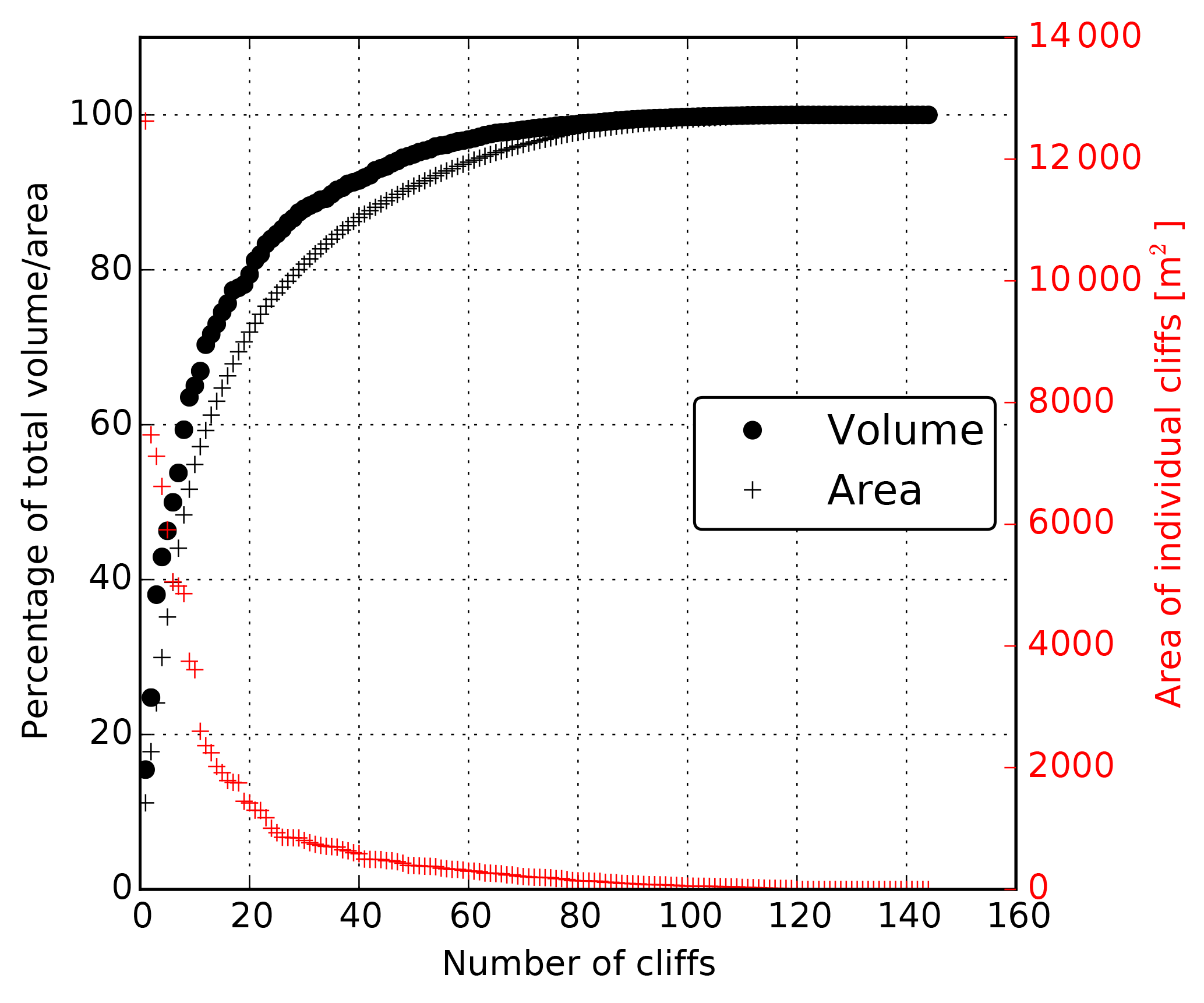
Figure 8 Individual ice cliff contributions for the period November 2015–November 2016 based on the UAV data. The left axis shows the cumulative volume (black dots) and area (black crosses), expressed as a percentage of the total volume or area. The right axis shows the area of individual cliffs (red crosses).

For individual cliffs, the contribution of the glacier-flow corrections were small relative to the uncertainties (Fig. 7), except for cliffs 11 and 12, which experienced a small volume change. These two cliffs are also located in the fastest-flowing part of the glacier tongue. The low magnitude of the glacier-flow correction is a result of (1) the small displacements of most of the cliffs and (2) the vertical displacement due to slope, which tended to compensate for the emergence velocity (Fig. 3). Nevertheless, for the two smallest and fast-moving cliffs (cliffs 11 and 12), these corrections were much larger and resulted in improved estimates of volume change for both Pléiades and UAV data (Fig. 7).

5.4 Total contribution of ice cliffs to net ablation over the glacier tongue, November 2015–November 2016

In addition to the 12 cliffs mapped in the field, we manually mapped 132 additional ice cliffs from the Pléiades and UAV orthoimages and slope maps. The total map view cliff footprint area from November 2015 to November 2016 was $\mathrm{113}\pm \mathrm{21}\times {\mathrm{10}}^{\mathrm{3}}$ m², i.e. 7.4 % of the total tongue map view area. Averaged over this cliff mask, the UAV (Pléiades) rate of elevation change corrected from glacier flow and emergence was $-\mathrm{3.88}\pm \mathrm{0.27}$ m a⁻¹ ($-\mathrm{3.91}\pm \mathrm{0.36}$ m a⁻¹). This corresponds to a total average volume loss at ice cliffs of $\mathrm{440}\pm \mathrm{54}\times {\mathrm{10}}^{\mathrm{3}}$ m³ a⁻¹.

The three largest cliffs contribute to almost 40 % of the total net ablation from cliffs (Fig. 8). As there is some variability in the rate of cliff thinning, the volume change of each cliff is not always directly related to its area (Figs. 8 and 9). Nevertheless, the largest cliffs dominate the volume loss, as 80 % of the total cliff contribution originates from the 20 largest cliffs in our study and all the cliffs below 2000 m² (i.e. the 120 smallest cliffs) contribute to less than 20 % of the total volume loss (Fig. 8).

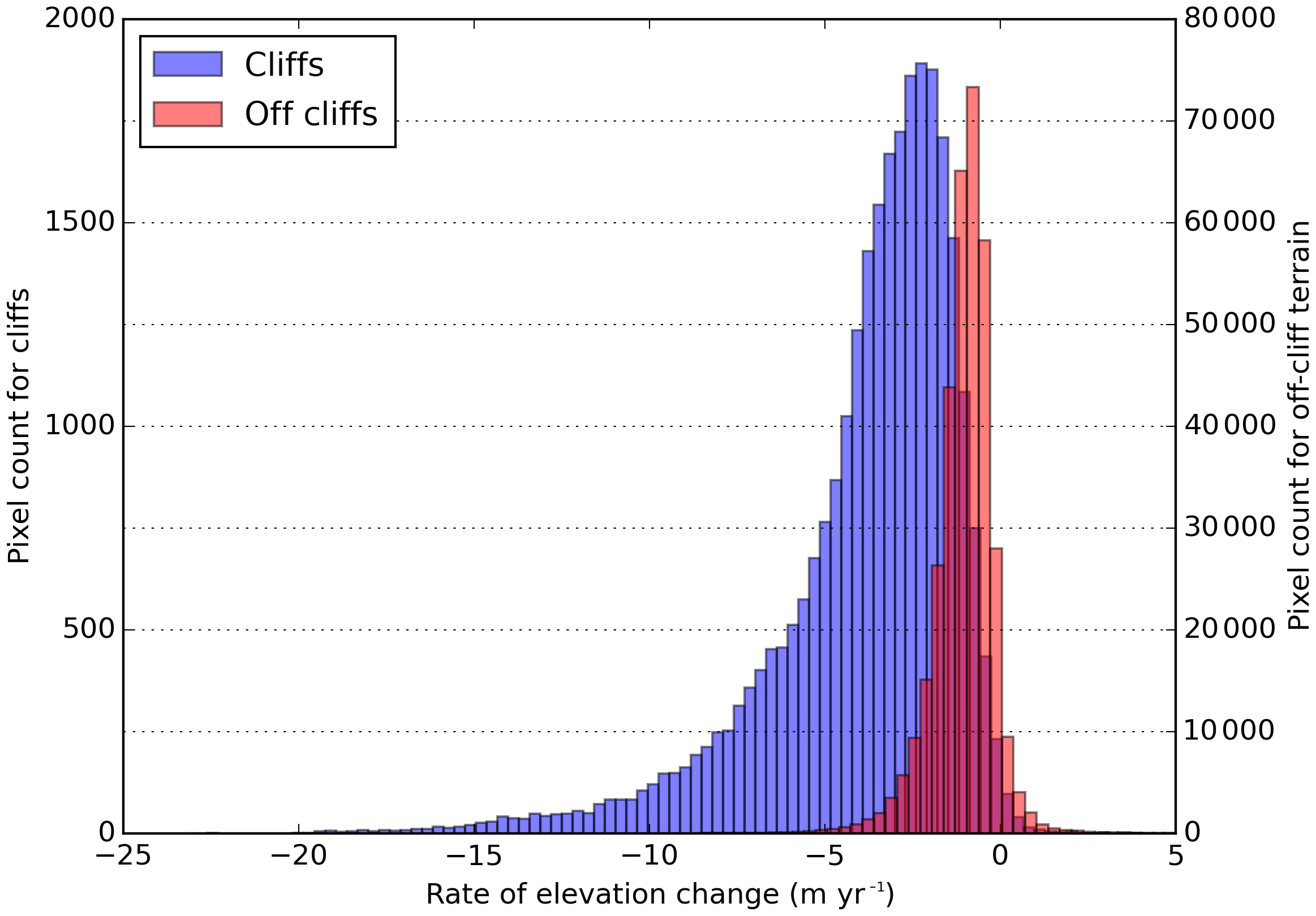
Figure 9 Rate of glacier surface elevation change for cliff and off-cliff terrain (Pléiades DEM difference November 2015–November 2016, corrected from flow). Note the strongly different y axis.

For the same period the tongue-averaged rate of elevation change was $-\mathrm{0.79}\pm \mathrm{0.21}$ m a⁻¹ (average of the UAV and Pléiades thinning rates). After adding the emergence velocity, this corresponds to a net glacier tongue ablation of 1.12±0.21 m a⁻¹ or a volume loss of $\mathrm{1.9}\pm \mathrm{0.2}\times {\mathrm{10}}^{\mathrm{6}}$ m³ a⁻¹. Consequently, the fraction of total net glacier tongue ablation due to cliffs was 23±5 %. These cliffs covered only 7.4 % of the tongue area. The factors f_C and $f_{\mathrm{C}}^{\ast }$ were thus equal to 3.1±0.6 and 3.7±0.7.

5.5 Total contribution of ice cliffs to net ablation over the glacier tongue, November 2016–November 2017

For the period November 2016–November 2017, we relied on the Pléiades and UAV data only. The cliff footprint area from November 2016 and November 2017 was $\mathrm{120}\pm \mathrm{21}\times {\mathrm{10}}^{\mathrm{3}}$ m², i.e. 7.8 % of the total tongue area. Averaged over this cliff mask, the UAV (Pléiades) rate of elevation change corrected for glacier flow and emergence was $-\mathrm{4.76}\pm \mathrm{0.27}$ m a⁻¹ ($-\mathrm{4.43}\pm \mathrm{0.36}$ m a⁻¹). The average from the Pléiades and UAV data gives a total ice cliff volume loss of $\mathrm{550}\pm \mathrm{66}\times {\mathrm{10}}^{\mathrm{3}}$ m³ a⁻¹.

The average thinning rate over the terminus was $-\mathrm{1.18}\pm \mathrm{0.21}$ m a⁻¹ (average of the UAV and Pléiades thinning rates). This corresponds to a net glacier tongue ablation of 1.51±0.21 m a⁻¹ after correction for the emergence or a total volume loss of $\mathrm{2.3}\pm \mathrm{0.2}\times {\mathrm{10}}^{\mathrm{6}}$ m³ a⁻¹. Consequently, between 2016 and 2017, ice cliffs contributed to 24±5 % of the net glacier tongue ablation. The factors f_C and $f_{\mathrm{C}}^{\ast }$ were thus equal to 3.0±0.6 and 3.6±0.7.

6 Discussion

6.1 Cliff evolution and comparison of 2 years of acquisition

The total area covered by ice cliffs did not vary significantly from year to year, ranging from $\mathrm{70}\pm \mathrm{14}\times {\mathrm{10}}^{\mathrm{3}}$ m² in November 2015 and 2017 to $\mathrm{71}\pm \mathrm{14}\times {\mathrm{10}}^{\mathrm{3}}$ m² in November 2016. The 12 individual cliffs surveyed showed substantial variations in area within the course of 1 year, with a maximum increase of 57 % for cliff 06 and a decrease of 34 % for cliffs 03 and 09 (Table S2). The total area of these 12 cliffs increased by 8 % in 1 year. Interestingly, over the same period, Watson et al. (2017) observed only a decline in ice cliff area on the tongue of Khumbu Glacier (∼6 km away), suggesting a lack of regional consistency. All the large cliffs (most of them are included in the 12 cliffs surveyed with the terrestrial photogrammetry) persisted over 2 years of survey, including the south or south-west-facing ones (Table 1), although south-facing cliffs are known to persist less than non-south-facing ones (Buri and Pellicciotti, 2018). However, we observed the appearance and disappearance of small cliffs, and terrain that was difficult to classify as cliff or non-cliff, highlighting the challenge in mapping regions covered by thin debris (Herreid and Pellicciotti, 2018).

We calculated backwasting rates for the 12 cliffs monitored with terrestrial photogrammetry for the period November 2015–November 2016 (Table 1). The backwasting rate is sensitive to cliff area changes (because it is calculated as the rate of volume change divided by the mean 3-D area) and should be interpreted with caution for cliffs that underwent large area changes (e.g. cliffs 01, 02, 03, 06, 09 and 11; Table S2). The backwasting rates ranged from 1.2±0.4 to 7.5±0.6 m a⁻¹, reflecting the variability in terms of ablation rates among the terrain classified as cliff (Fig. 9). The lowest backwasting rates are observed for cliffs 11 and 12, located on the upper part of the tongue, roughly 100 m higher than the other cliffs (Fig. 1 and Table 1). The largest backwasting rates were observed for cliff 01, which expanded significantly between November 2015 and November 2016. The backwasting rates are lower than those reported by Brun et al. (2016) on Lirung Glacier (Langtang catchment) for the period May 2013–October 2014, which ranged from 6.0 to 8.4 m a⁻¹ and lower than those reported by Watson et al. (2017) on Khumbu Glacier for the period November 2015–October 2016, which ranged from 5.2 to 9.7 m a⁻¹ (we reported the values for cliffs which survived over their entire study period only). These differences are likely due to temperature differences between sites. Indeed, the cliffs studied here are at higher elevation (5320–5470 m a.s.l.) than the two other studies (4050–4200 m a.s.l. for Lirung Glacier and 4923–4939 m a.s.l. for Khumbu Glacier).

While a comparison between only 2 years of data cannot be used to extrapolate our results in time, we note the similarity between the total ice cliff contribution and net ablation (23±5 % and 24±5 % in November 2015–November 2016 and November 2016–November 2017). In contrast, total net ablation of the Changri Nup Glacier tongue was ∼25 % higher for the period November 2016–November 2017 than for the period November 2015–November 2016. While a difference in meteorological conditions between these 2 years is a likely cause of the greater ablation totals, the ice cliffs seem to contribute a constant share to the total ablation.

6.2 Influence of emergence velocity and glacier-flow correction on f_C and $f_{\mathrm{C}}^{\ast }$

In most studies quantifying ice cliff ablation (Brun et al., 2016; Thompson et al., 2016), the glacier thinning rate was assumed to be directly equal to the net ablation rate; i.e. emergence velocity was assumed to be zero. If we make the same assumption (but still include the corrections for horizontal displacement and the vertical displacement due to the slope), we find a mean thinning rate of 0.80±0.10 m a⁻¹ for the tongue and of 3.59±0.17 m a⁻¹ for the cliffs (average of UAV and Pléiades data) for the period November 2015–November 2016. This results in calculated values of $f_{\mathrm{C}}=\mathrm{4.5}\pm \mathrm{0.6}$ (and $f_{\mathrm{C}}^{\ast }=\mathrm{5.4}\pm \mathrm{0.7}$), which is 50 % higher than the actual value. Ice cliffs would thus contribute to ∼34 % of the total tongue ablation. For the period November 2016–November 2017, the same assumption results in $f_{\mathrm{C}}=\mathrm{3.6}\pm \mathrm{0.6}$ (and $f_{\mathrm{C}}^{\ast }=\mathrm{4.3}\pm \mathrm{0.7}$), and an ice cliff contribution of ∼29 % to the total tongue ablation. Neglecting w_e might partially explain why previous studies found significantly higher values of f_C, and our results stress the need to estimate and take into account ice flow emergence, even for nearly stagnant glacier tongues like Changri Nup Glacier (see Discussion below).

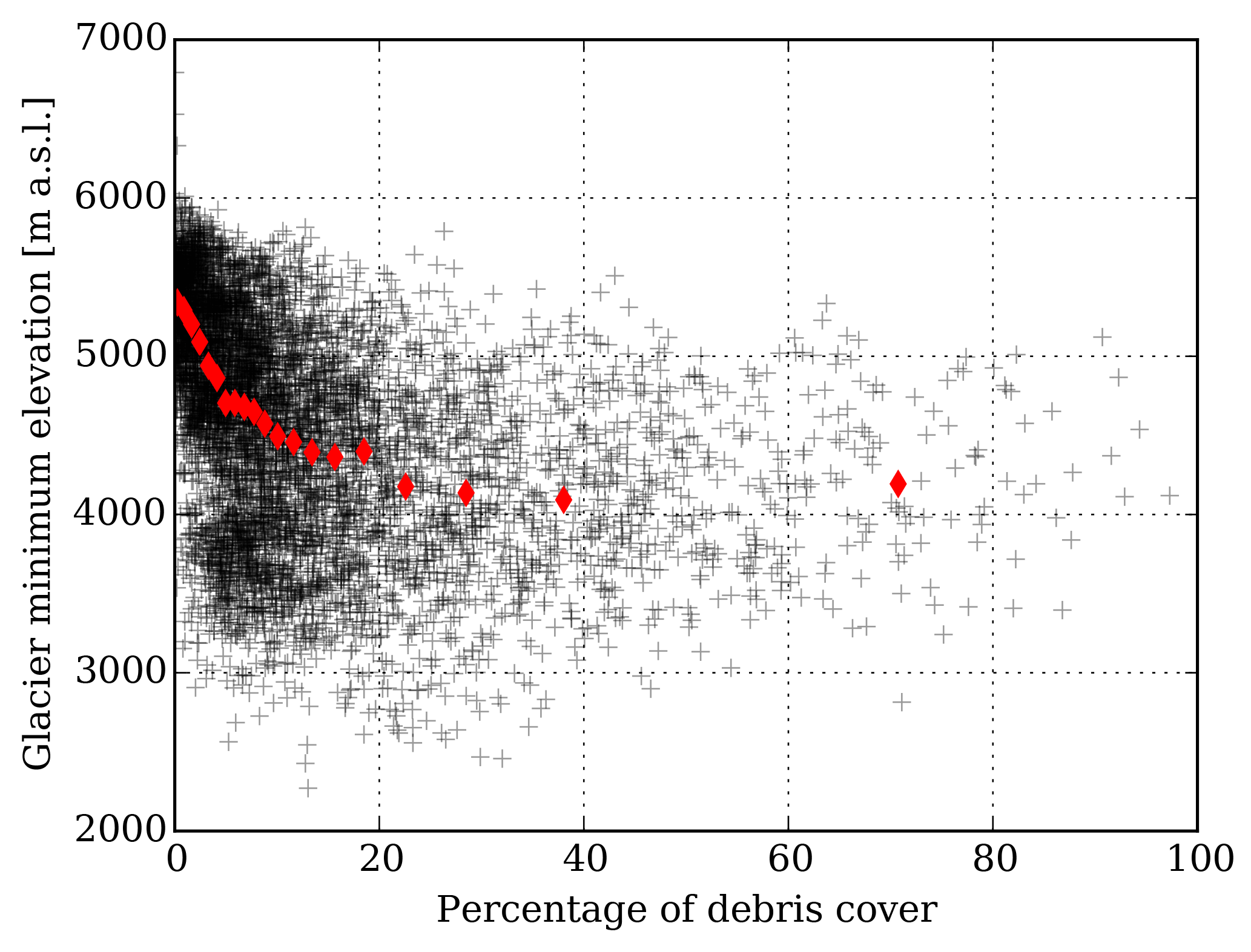
Figure 10 Glacier minimum elevation as a function of the percentage of debris cover for the glaciers larger than 2 km² in high-mountain Asia (6571 glaciers in total). The black crosses represent individual glaciers and the red diamonds show the mean of the glacier minimum elevation for each 5th percentile of debris cover. For instance, the first diamond represents the mean of the glacier minimum elevation for glaciers with a percentage of debris cover between 0 (minimum) and 0.51 % (5th percentile).

Values of f_C and $f_{\mathrm{C}}^{\ast }$ not corrected for the emergence velocity can be compared to the previous observational estimates. Both Brun et al. (2016) and Thompson et al. (2016) found values higher than our estimates. Part of the difference might arise from the different climatological settings, as Lirung and Ngozumpa glaciers are located at lower elevation than Changri Nup Glacier.

6.3 Ice cliff ablation and the debris-cover anomaly

Between November 2011 and November 2015, Vincent et al. (2016) quantified the reduction in area-averaged net ablation over the glacier tongue due to debris-cover. They obtained tongue-wide net ablations of −1.2 and −3.0 m w.e. a⁻¹ with and without debris. As demonstrated in this study, ice cliffs ablate at −3.5 m w.e. a⁻¹, ∼3.6 times faster than the non-cliff terrain of the debris-covered tongue for the period November 2015–November 2016, and ∼1.2 times faster than the tongue if it was entirely debris-free. Consequently, approximately 75 % of the tongue would have to be covered by ice cliffs to compensate for the lower ablation rate under debris and to achieve the same overall ablation rate as a clean ice glacier under similar conditions. Since ice cliffs typically cover a very limited area (Herreid and Pellicciotti, 2018), it is unlikely that they can enhance the ablation of debris-covered tongues enough to reach the level of ablation of ice-free tongues.

Other ablation-related processes such as supraglacial ponds (Miles et al., 2016) or englacial ablation (Benn et al., 2012) may contribute to higher ablation rates than what can be expected on the basis of the Østrem curve. Yet the contribution of these processes is not sufficient to enhance the ablation of the debris-covered tongue of Changri Nup Glacier at the level of clean ice ablation, as Vincent et al. (2016) already showed that the insulating effect of debris dominates for this glacier. As a consequence, and based on this case study, we hypothesize that the reason for similar thinning rates over debris-covered and debris-free areas, i.e. the debris-cover anomaly, is largely related to a reduced emergence velocity compensating for reduced ablation due to the debris mantle.

This hypothesis currently applies to the Changri Nup Glacier tongue only, and it is unclear if it can be extended to the debris-cover anomaly identified on larger scales. The high-quality data available for Changri Nup Glacier are not available for other glaciers at the moment, and we thus provide a theoretical discussion below.

The mass-conservation equation (Cuffey and Paterson, 2010) gives the link between thinning rate ($\stackrel{\mathrm{‾}}{\frac{\partial h}{\partial t}}$ in m a⁻¹), ablation rate and emergence velocity for a glacier tongue:

$$\begin{array}{}\text{(10)}& \stackrel{\mathrm{‾}}{{\displaystyle \frac{\partial h}{\partial t}}}=-{\displaystyle \frac{\mathrm{1}}{\mathit{\rho }}}\dot{b}+{\displaystyle \frac{\mathrm{\Phi }}{A}},\end{array}$$

where Φ (m³ a⁻¹) is the ice flux entering the tongue of area A (m²), ρ is the ice density (kg m⁻³), and $\dot{b}$ is the area-averaged tongue net ablation (kg m⁻² a⁻¹ or m w.e. a⁻¹).

Consider two glaciers with tongues that are either debris-covered (case 1- referred hereafter as “DC”) or debris-free (case 2 – referred hereafter as “DF”), and similar ice fluxes entering the ELA i.e. Φ_DC=Φ_DF. The ice flux at the ELA is expected to be driven by accumulation processes, and it is reasonable to assume similarity for both debris-covered and debris-free glaciers. There is a clear link between the glacier tongue area and its mean emergence velocity: the larger the tongue, the lower the emergence velocity. These theoretical considerations have been developed by Banerjee (2017) and Anderson and Anderson (2016), the latter demonstrating that debris-covered glacier lengths could double, depending on the debris effect on ablation in their model. Real-world evidence for such differences in debris-covered and debris-free glacier geometry remain largely qualitative. For instance, Scherler et al. (2011) found lower accumulation-area ratios for debris-covered than debris-free glaciers. Additionally, based on the data of Kraaijenbrink et al. (2017), we found a negative correlation ($r=-\mathrm{0.36}$, p<0.01) between the glacier minimum elevation and the percentage of debris cover (Fig. 10). The combination of these two observations hints at both reduced ablation and a larger tongue for debris-covered glaciers.

Consequently, the qualitative picture we can draw is that the ablation area of glaciers with considerable debris cover is usually larger than for debris-free glaciers (A_DC>A_DF). This results in lower emergence velocities ($w_{\mathrm{e},\text{DC}}=\mathrm{\Phi }/A_{\text{DC}}<\mathrm{\Phi }/A_{\text{DF}}=w_{\mathrm{e},\text{DF}}$). If the glacier is in mass and dynamical equilibrium, in both debris-covered and debris-free cases, the thinning rate at any elevation is 0, because the emergence velocity compensates for the surface mass balance. However, both w_e and $\dot{b}$ will be lower for the debris-covered tongue (Fig. 11). In an unbalanced regime with consistent negative mass balances, as mostly observed in high-mountain Asia (Brun et al., 2017), similar thinning rates between debris-free and debris-covered tongues could be the combination of reduced emergence velocities and lower ablation for debris-covered glaciers (Fig. 11). Evidence for reduced debris-covered glacier velocities and loss of connectivity between accumulation and ablation areas (Neckel et al., 2017) will lead to further reductions in both ice fluxes and w_e.

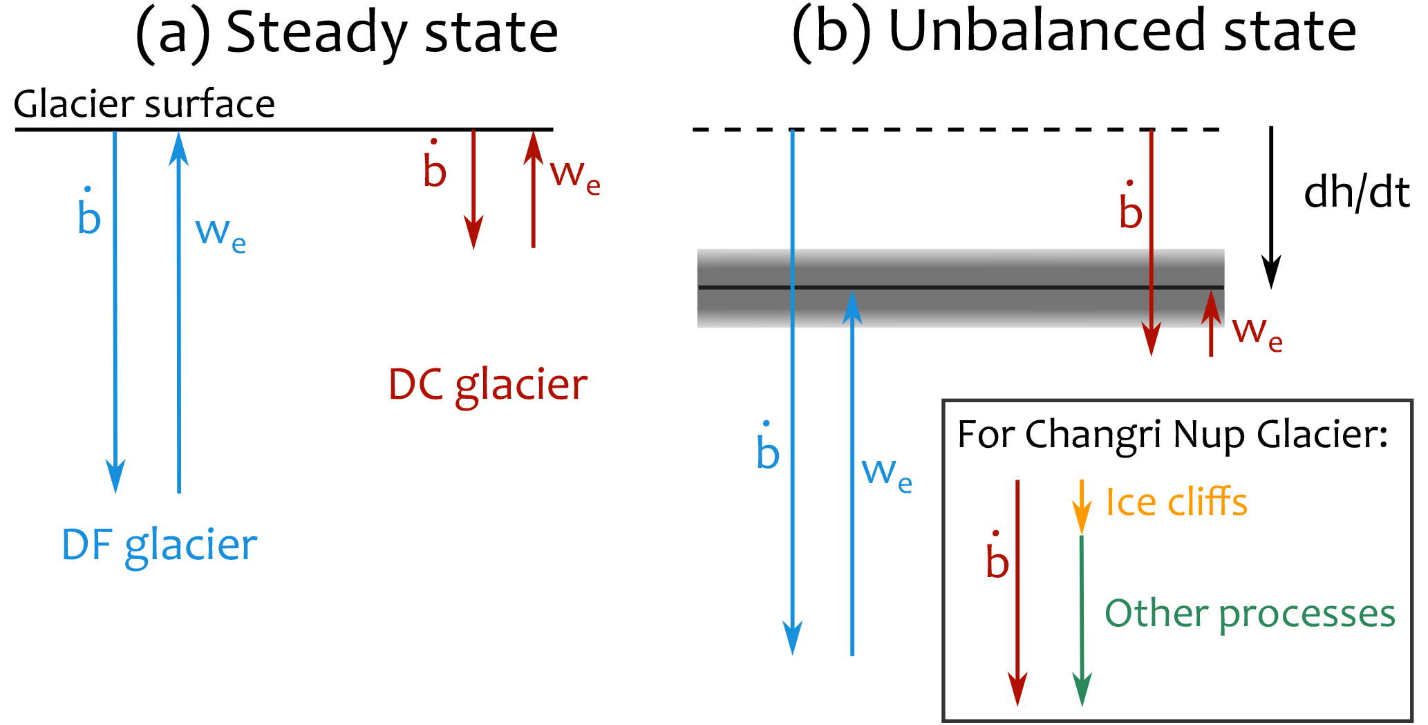
Figure 11 Conceptual representation of the interplay of net ablation ($\dot{b}$) and emergence velocity (w_e) for debris-free (DF, blue) and debris-covered (DC, brown) glacier tongues. In the left panel both glaciers are at equilibrium (no thinning) and in the right panel their tongues are thinning at roughly the same rate $\stackrel{\mathrm{‾}}{\partial h/\partial t}$, shown by the grey-shaded area. In the unbalanced state, the values are scaled according to Vincent et al. (2016). For the steady state, we assumed a similar emergence velocity for the debris-free tongue. The inset shows the share of the ice cliffs versus the other processes for the tongue-wide ablation on Changri Nup Glacier tongue. It is noteworthy that this representation is only conceptual, that it is based on our current understanding of the interplay of ablation and ice dynamics of a single small glacier tongue (Changri Nup), and that the emergence velocity values are very poorly constrained.

In conclusion, our field evidence shows that enhanced ice cliff ablation alone could not lead to a similar level of ablation for debris-covered and debris-free tongues. While other processes can substantially increase the ablation of debris-covered tongues, we highlight the potentially important role of the neglected emergence velocity in the explanation of the debris-cover anomaly.

6.4 Applicability to other glaciers

Determining the total ice cliff contribution to the net ablation of the tongue (i.e. the f_C factor defined in this study) of a single glacier has limited value by itself, because we do not know the variability between glaciers. In particular, it is too early to conclude whether the range of f_C values reported in the literature reflects inconsistencies amongst the different methods or is actually a reflection of variability between glaciers. For instance, model-based f_C values (Buri et al., 2016b; Juen et al., 2014; Reid and Brock, 2014; Sakai et al., 1998) are not directly comparable with the observations (Brun et al., 2016; Thompson et al., 2016), because they usually require additional assumptions, e.g. about the sub-debris ablation or emergence velocity. The definition of debris-covered tongues, the nature of their surface and their hypsometry might also have a considerable effect on f_C.

A significant obstacle to applying our method to other glaciers is the need to estimate the emergence velocity, which requires an accurate determination of the ice fluxes entering the glacier tongues. The measurement of ice thickness with GPR systems is already challenging for debris-free glaciers, as it requires that the transmitter, receiver and antennas must be pulled along transects on the glacier surface. It is even more challenging for debris-covered glaciers, as the hummocky surface prevents the operators from dragging a sledge. More field campaigns dedicated to ice thickness and velocity measurements (Nuimura et al., 2011, 2017) or the development of airborne ice thickness retrievals through debris are needed, as stressed by the outcome of the Ice Thickness Models Intercomparison eXperiment (Farinotti et al., 2017). The precise retrieval of emergence velocity pattern using a network of ablation stakes combined with DGPS is a promising alternative, in particular if combined with detailed ice flow modelling (Gilbert et al., 2016).

7 Conclusions

In this study, we estimate the total contribution of ice cliff to the total net ablation of a debris-covered glacier tongue for two consecutive years, taking into account the emergence velocity. Ice cliffs are responsible for 23–24±5 % of the total net ablation for both years, despite a tongue-wide net ablation that is approximately 25 % higher in the second year. On Changri Nup Glacier, the fraction of total net ablation from ice cliffs is too low to explain the debris-cover anomaly. Other contributions, such as ablation from supraglacial lakes or along englacial conduits, are potentially large and have yet to be quantified. For the specific case of Changri Nup Glacier they are likely not large enough to compensate for the reduced ablation (Vincent et al., 2016). Consequently, we hypothesize that the debris-cover anomaly could be a result of lower emergence velocities and reduced ablation, which leads to thinning rates comparable to those observed on clean ice glaciers. However, ice cliffs are still hotspots of ablation and consequently of enhanced thinning; without them, the thinning rates of debris-covered and clean ice might not be similar.

Our method requires high-resolution UAV or satellite stereo imagery and is restricted to glaciers where thickness estimates at a cross section upstream of the debris-covered tongue are available, and emergence velocity can be estimated. A comparison of cliff ablation enhancement factor (f_C or $f_{\mathrm{C}}^{\ast }$) values calculated for other debris-covered glaciers under our suggested framework would inform a comparison of estimates of ice cliff ablation for other and potentially much larger debris-covered tongues. Though our results cover only 2 years of data where net ablation totals differed by 25 %, the area occupied by ice cliffs and their relative contribution to ablation (f_C) remained almost constant. A main limitation of our study is its short spatial and temporal extent, and it would be worthwhile to obtain longer-term estimates of the relative ice cliff contribution to net ablation at multiple sites. These estimates would lead to the development of empirical relationships for cliff enhanced ablation that could be included in debris-covered glacier mass-balance models.

In line with a previous study (Vincent et al., 2016), we stress the need for more research about the emergence velocity of debris-covered (and nearby debris-free) tongues, as the assumption that thinning rates are equal to net ablation rates is incorrect and can lead to inaccurate conclusions. Two research directions could be (a) to measure cross-sectional ice thicknesses for multiple debris-covered glaciers and (b) to install dense networks of ablation stakes to assess the spatial variability of ice flow emergence.