the Creative Commons Attribution 4.0 License.
the Creative Commons Attribution 4.0 License.
 | 18 Jul 2018
Circumpolar patterns of potential mean annual ground temperature based on surface state obtained from microwave satellite data
Christine Kroisleitner
Helena Bergstedt
Gap filling is required for temporally and spatially consistent records of land surface temperature from satellite data due to clouds or snow cover. Land surface state, frozen versus unfrozen conditions, can be, however, captured globally with satellite data obtained by microwave sensors. The number of frozen days per year has been previously proposed to be used for permafrost extent determination. This suggests an underlying relationship between number of frozen days and mean annual ground temperature (MAGT). We tested this hypothesis for the Northern Hemisphere north of 50∘ N using coarse-spatial-resolution microwave satellite data (Metop Advanced SCATterometer – ASCAT – and Special Sensor Microwave Imager – SSM/I; 12.5 and 25 km nominal resolution; 2007–2012), which provide the necessary temporal sampling. The MAGT from GTN-P (Global Terrestrial Network for Permafrost) borehole records at the coldest sensor depth was tested for validity in order to build a comprehensive in situ data set for calibration and validation and was eventually applied. Results are discussed with respect to snow water equivalent, soil properties, land cover and permafrost type. The obtained temperature maps were classified for permafrost extent and compared to alternative approaches.
An R2 of 0.99 was found for correlation between and MAGT at zero annual amplitude provided in GTN-P metadata and MAGT at the coldest sensor depth. The latter could be obtained with an RMSE of 2.2 ∘C from ASCAT and 2.5 ∘C from SSM/I surface state records using a linear model. The average deviation within the validation period is less than 1 ∘C at locations without glaciers and coastlines within the resolution cell in the case of ASCAT. The exclusion of snow melt days (available for ASCAT) led to better results. This suggests that soil warming under wet snow cover needs to be accounted for in this context. Specifically Scandinavia and western Russia are affected. In addition, MAGT at the coldest sensor depth was overestimated in areas with a certain amount of organic material and in areas of cold permafrost. The derived permafrost extent differed between the used data sets and methods. Deviations are high in central Siberia, for example. We show that microwave-satellite-derived surface state records can provide an estimation of not only permafrost extent but also MAGT without the need for gap filling. This applies specifically to ASCAT. The deviations among the tested data sets, their spatial patterns as well as in relation to environmental conditions, revealed areas which need special attention for modelling of MAGT.
- Article
(6855 KB) - Full-text XML
- BibTeX
- EndNote


Permafrost covers large parts of the Earth's surface and is defined as ground that remains at or below 0 ∘C for at least 2 consecutive years. The impact of climate change on the Arctic, as well as other permafrost-dominated environments, is thought to be more severe compared to the rest of the world (National Research Council, 2013; Schuur et al., 2015). Warming and with that thawing of permafrost impacts multiple environmental processes ranging from surface and sub-surface hydrology (O'Donnell et al., 2012; Woo et al., 2008), ecological changes (Schuur et al., 2008) to processes like carbon exchange (Hayes et al., 2014). Knowledge of the temperature of the ground, the extent of permafrost and possible changes in its distribution are therefore crucial for climate modelling and prediction (Cheng and Wu, 2007; O'Connor et al., 2010). So far, the exact extent of permafrost is unknown and has only been approximated (Nguyen et al., 2009; Zhang et al., 2008).
A range of approaches exist for modelling mean annual ground temperature (MAGT) and subsequent permafrost extent determination. They vary in complexity and accuracy and their parameterization differs depending on the size of the area of interest and data availability. Different temperature data sources are employed for the approximation. For example Gruber (2012) has used reanalysis records, which are based on spatially interpolated in situ air temperature data (mean annual air temperature) together with elevation data (lapse rate), to generate a global map of permafrost probabilities. Temperature records from reanalyses and land surface temperature from satellites together with basic vegetation information and satellite-derived snow properties have been investigated by Westermann et al. (2015) for modelling larger areas as satellite data alone do not provide the required spatially and temporally consistent temperature values. Cloud cover is problematic when using thermal infrared. Clear-sky bias is an additional problem (Soliman et al., 2012). Improved temperature records can be obtained for the snow-free period from combination with passive microwave data (André et al., 2015). Such records need to be, however, complemented with reanalysis data for the remaining year in case of further analyses that target MAGT.
An approach for permafrost extent determination without estimation of MAGT and use of satellite records has only been recently described by Park et al. (2016). They have hypothesized that the number of frozen days per year from passive microwave satellite data (SSM/I – Special Sensor Microwave Imager) can be used as indicator for permafrost extent. A 30-year record was analysed for trends and compared to the map of Brown et al. (1997) – often referred to as the IPA (International Permafrost Association) map – and results of a coupled hydrological and biogeochemical model (Park et al., 2011a). A threshold of half a year of frozen days during at least 2 consecutive years was chosen to delineate possible permafrost areas. This value was justified with reference to Dobinski (2011), Nelson and Outcalt (1987), Saito et al. (2013), and Zhang et al. (2005). These studies have used measures derived from actual temperature records, specifically the use of mean annual air temperature and the concept of thawing–freezing degree days. Results showed differences between the model and microwave product, especially at the start of the record, which could be due to sparse satellite data during the beginning of the chosen time period (Trofaier et al., 2017). The comparison with the IPA permafrost map revealed an overestimation of permafrost extent around 65∘ N. Overall, agreement regionally differed, especially over non-continuous permafrost. Luoto et al. (2004) suggested that the minimum number of frozen days is 200 for new permafrost to develop (in the form of palsas) in the transition zone of Scandinavia. Additionally, local factors like a low annual mean air temperature (< 1 ∘C), water-saturated peat, moss patches and low vegetation have to be present (Harris, 1981; Seppälä, 1986). This number is considerably higher compared to the selection of Park et al. (2016). The utility of a single threshold may, however, be the result of an underlying relationship between MAGT and number of frozen days.
Surface state information, and with that the calculation of frozen and thawed days per year, can also be derived from active microwave sensors operating at various frequencies (Bartsch et al., 2007; Naeimi et al., 2012; Park et al., 2011b; Wang et al., 2008; Zwieback et al., 2015). Frequencies are usually lower than those measured by SSM/I, and especially C-band (5.3 GHz) scatterometers like the ASCAT (Advanced SCATterometer) sensor on-board the Metop satellites have already been shown to be applicable for freeze–thaw information retrieval in permafrost regions by validation with near-surface soil temperature from borehole records (Naeimi et al., 2012). Multi-annual statistics of thaw and freeze-up timing based on these records have been applied for the retrieval of circumpolar landscape units, for example (Bartsch et al., 2016b).
The number of frozen days can be observed consistently from space. Freezing degree days, as conventionally used for MAGT retrieval, require spatial and temporal interpolation and gap filling of available temperature data (both in situ and from satellites). The use of frozen days would therefore allow a purely observation-based assessment. This does, however, require the assumption that changes at the surface (as represented by the satellite at a certain frequency) are uniformly and linearly related to sub-ground temperatures. This neglects effects such as insulation by snow as well as varying soil thermal conductivity. The validity of the approach may therefore be limited. In cases in which it is applicable, the approach may, however, allow the estimation of actual ground temperatures and not only extent.
A further issue is the available data for calibration and validation of data sets spanning the entire Arctic. The map of Brown et al. (1997) does provide zones of permafrost occurrence which correspond to area fraction of permanently frozen ground. The actual patterns within the non-continuous zone are unknown; different sources have been used and it represents the state of the second half of the 20th century. Results need to be therefore treated with care. The study of Brown et al. (1997) is however used in many studies for evaluation of modelling results (Matthes et al., 2017; Park et al., 2016).
An alternative is actual ground temperature measurements. Borehole data only represent, however, point information, with uneven distribution (Biskaborn et al., 2015) and they provide measurements at selected depths only. The MAGT derived from these records is currently only provided in some cases by the data owners within the Global Terrestrial Network on Permafrost (GTN-P) database. A practical method which allows the use of all freely available data is required for circumpolar applications.
The objective of this study is to investigate the applicability of the frozen day approach based on satellite data for potential permafrost extent determination as well as MAGT retrieval. Special emphasis is given on suitability of calibration and validation data, differences among microwave sensors, and uncertainties with respect to environmental conditions including snow, land cover and ground ice content. Regional patterns of agreement with the map of Brown et al. (1997) as well as with in situ data are discussed.
2.1 Satellite records
We used two microwave remote-sensing data sets derived from globally available records and with similar classification accuracy obtained by comparison to air temperature data. They were derived from sensors with different frequencies, acquisition methods (active versus passive) and timing. The first was derived from the ASCAT sensor on-board the Metop satellites. The ASCAT sensor is a C-band (5.255 GHz) scatterometer (Figa-Saldaña et al., 2002), providing almost daily coverage of the Earth's surface. The Equator overpass time is 09:30 local solar time (LST). The surface state information (freeze–thaw) was derived from the ASCAT sensor as a surface status flag for a soil moisture product specifically post-processed for high latitudes (Paulik et al., 2014). The circumpolar data set covers the years 2007–2013. It was developed for permafrost monitoring and climate modelling purposes (Bartsch and Seifert, 2012; Naeimi et al., 2012; Reschke et al., 2012) and covers the area above 50∘ N with a grid spacing of 12.5 km and an up-to-daily temporal resolution (Paulik et al., 2014). This includes the parameters frozen and thawed ground, temporary water (including snow melt), and frozen water/permanent ice. The surface status information was derived using a stepwise threshold algorithm based on ASCAT backscatter values and ECMWF reanalysis data (Naeimi et al., 2012). The accuracy was assessed with in situ surface air temperature measurements from the global weather station network and found to be about 82 % overall (Naeimi et al., 2012). Up to 92 % agreement was found for near-surface temperature measurements from boreholes of GTN-P located in Siberia.
The second remotely sensed data set used in this study was derived from global daily (ascending and descending orbit) 37 GHz vertically polarized brightness temperature observations from calibrated SMMR (Scanning Multichannel Microwave Radiometer) and SSM/I satellite sensor records by Kim et al. (2014). There have been a series of these sensors carried on-board satellites from the Defense Meteorological Satellite Program. They are passive radiometric systems that measure atmospheric, ocean and terrain microwave temperature (Hollinger et al., 1990). SSM/I equatorial crossings are 06:00 and 18:00 LST. The freeze–thaw status was analysed globally from 1979 to 2012 by Kim et al. (2014). The data set has a nominal resolution of 25 km and covers the Arctic terrestrial drainage basin. The actual footprint size at 37 GHz is 37 km × 28 km. The threshold approach produces two classes: frozen and non-frozen. The estimated classification accuracy is approximately 85 % (morning passes) to 92 % (afternoon passes) compared to in situ surface air temperature measurements from the global weather station network (Kim et al., 2012). This data set was used by Park et al. (2016) for the assessment of permafrost extent changes.
2.2 In situ records from boreholes
All borehole records above a latitude of 50∘ N with available time series of ground temperature were retrieved from the Global Terrestrial Network for Permafrost database (GTN-P, 2016). The network collects measurements of the thermal state of permafrost (TSP) in polar and mountain regions. A total of 277 borehole sites have temperature data; single sites often comprise more than one measurement unit or period, which leads to a total sum of 1062 ground temperature data sets (Biskaborn et al., 2015). The depth of most boreholes is less than 25 m, although the average is 53 m. The most frequent sensor depth can be found at 5 m. Romanovsky et al. (2010) reported that measurement systems currently in use generally provide an accuracy and precision of 0.1 ∘C or better. The time series are available in hourly, daily or annual resolution and cover different time periods. The deepest sensor depths of the used data set vary between 1 and 99 m. In total, 216 boreholes were considered. There were however inconsistencies in sensor spacing and the MAGT at zero annual temperature amplitude was not directly measured. Most records of North America are accompanied with meta-records, which suggest a sensor depth (closest to zero annual temperature amplitude) for approximation of the MAGT. But this information is unavailable for the majority of records from Asia. MAGT values together with the year they represent are available for 64 sites only (24 % of all sites relevant for the analysis period). The boreholes represent a MAGT range from −15 to 6 ∘C.
2.3 Spatial information on environmental conditions
The circumpolar permafrost map by Brown et al. (1997) depicts the permafrost extent divided into different classes as well as the ground ice content for the Northern Hemisphere (20 to 90∘ N). The data set defines permafrost as frozen ground that remains at or below 0 ∘C for at least 2 years. Areas are classified as continuous, discontinuous, sporadic or isolated permafrost with differing ground ice content. The classes correspond to percent area categories: 90–100, 50–90, 10–50, < 10 % and no permafrost. These classes were compared separately and as one aggregated class (excluding areas of no permafrost) to the results of the frozen day classifications. Zones with specified ground ice content are also supplied with the permafrost map and used in this study. Classes are high > 20 %, medium 10–20 % and low < 10 %.
The Global Snow Monitoring for Climate Research (GlobSnow) data set provides information about snow water equivalent (SWE) and snow extent for the Northern Hemisphere (25–84∘ N) (GlobSnow, 2015; Metsämäki et al., 2015). The products are based on SMMR, SSM/I and AMSR-E sensor data in combination with ground-based measurements (GlobSnow, 2015; Takala et al., 2011). The SWE data product used in this study has a spatial resolution of 25 km. The SWE values are provided as daily SWE, weekly aggregated SWE and monthly aggregated SWE. In this study, we used the monthly aggregated SWE, which provides a maximum SWE value for each month to determine the maximum SWE for each winter.
The Global Land Cover 2000 Project (GLC 2000) provides global land cover information at 1 km resolution (GLC2000, 2003). The data are mainly based on Satellite Pour l'Observation de la Terre-4 (SPOT-4) observations, partially supported by other Earth observing sensors (Bartholomé and Belward, 2005).
We extracted the soil texture for all points from the Harmonized World Soil Database (Fischer et al., 2008) and soil organic carbon (SOC) from the Northern Circumpolar Soil Carbon Database (NCSCD) by Hugelius et al. (2013, 2014) to include the soil properties in our analysis. The NCSCD is a polygon-based digital database compiled from harmonized regional soil classification maps in which data on soils have been linked to pedon data from the northern permafrost regions to calculate SOC content and mass. It includes SOC values for 0–30, 0–100, 0–200 and 0–300 cm.
3.1 Preparation of borehole temperature data
The MAGT is usually calculated at the depth of zero annual amplitude (ZAA) for permafrost studies. As the availability of data at specific depths is limited, representing or reaching the depth of ZAA is not possible for all cases. The MAGT, defined as the temperature at a specific site in this study, was therefore calculated for each borehole location at the depth of the minimum MAGT. The minimum MAGT, in a stable climate, would be the same as the MAGT at the depth of ZAA (Bodri and Cermak, 2007). Where available, we have also collected metadata for all GTN-P boreholes regarding MAGT, the year of the calculation and the depth of the sensor representing MAGT in order to test the validity of this approach. The MAGT at the coldest sensor depth is referred to as MAGTc in the following. Only sensors instrumented below a depth of 1 m were used as the MAGT near the surface can be much colder than at a larger depth. Temperature time series of the different sensors were tested for gaps and inconsistencies. Only years with complete records were considered for calibration and validation. The used sites are located within an area with 150 to 330 frozen days as observed in the satellite records in order to account for artifacts which can occur due to large water bodies within the footprint, for example.
3.2 Preprocessing of satellite records
Both surface status data sets underwent post-processing before being used in our permafrost extent and temperature estimation.
The ASCAT surface status flag (SSF) data contain cells with no data for which the algorithm failed to produce a result. Gaps were filled by surrounding values (class with majority), ensuring a complete data set. The sum of frozen days per year for every pixel was determined for both satellite records, according to the method of Park et al. (2016). Grid cells in which the number of frozen days exceeds the number of thawed days during 2 consecutive years were classified as permafrost. We defined the averaging period with respect to the water year from 1 September to 31 August as suggested by Park et al. (2016).
To explore the dependency of the results on snow melting events, the permafrost extent estimation from ASCAT data was carried out excluding the melt days in the count of frozen days (FT) and a second analysis counting the melt days as frozen days (FM).
3.3 Model parameterization for potential mean annual ground temperature retrieval
The relationship between MAGTc and frozen days per year was further examined for the retrieval of ground temperature and consecutive determination of permafrost extent by using the 0 ∘C threshold. Only data inside the range of 150 to 330 frozen days per year were considered. Additionally, sites which are located on islands in the high Arctic were excluded with respect to microwave sensor footprint size. The remaining 168 sites were used to fit the model. The records from ASCAT as well as SSM/I were split into two parts by defining a calibration (2009–2011) and a validation period (2007–2008). We tested linear, logarithmic and polynomial functions on their ability to describe the relationship between MAGTc and frozen days per year. We found no significant fit for polynomial functions and a slightly weaker fit for logarithmic functions compared to a simple linear regression. Therefore a linear model was applied to the frozen days for the years 2009 to 2011 for the determination of an empirical relationship. The resulting formula was used to estimate the MAGTc from the day of year data set for the years 2007 and 2008. The differences between the modelled and in situ MAGTc were calculated separately for the 2 years in order to assess the capability of the approach to capture inter-annual variations, to investigate various environmental impacts (snow water equivalent, land cover type), and differences between previously defined permafrost zones and specific regions. The Arctic was split into 14 regions in the latter case (Fig. 1).
The average MAGTc for the entire time period (2007–2011) was calculated for ASCAT FT and SSM/I results and compared. The standard deviation was derived in addition.

Figure 1Map of used GTN-P boreholes with region class. “No data” refers to sites without publicly available data or sites which failed the selection criteria. ANS – Alaska Highway transect and North Slope; ArcG – Canadian High Arctic and Greenland; CR – central Russia; NR – northern Russian Far East; SR – southern Russian Far East; Sva – Svalbard; Swe – Sweden; WA – western Alaska; WR – western Russia; YN – Yamalo-Nenets district; Yak – central and southern Yakutia; cSib – central Siberia; mCa – mainland Canada. For legend of permafrost extent (line features) see Fig. 15.
3.4 Frozen day threshold determination for potential permafrost extent
The modelled MAGTc values were also classified for each year in order to obtain permafrost extent maps (binary maps of values below and above 0 ∘C). Results were compared to two further approaches for threshold determination. In the study of Park et al. (2016) a threshold of half a year of frozen days was chosen for the delineation of permafrost extent. Half a year corresponds to 180 or 182.5 days in climate models (Saito et al., 2013). In the first step, we extended the analysis to 210 frozen days to test the validity of the suggested threshold. The cross comparison with the permafrost extent classes considered the information of four thresholds (180, 190, 200, 210) for the entire study area, which allowed us to analyse the difference in estimated permafrost extent and the sensitivity of this approach to the chosen threshold. The results from both active and passive microwave freeze–thaw data sets were compared with the permafrost map by Brown et al. (1997). To further evaluate the initial threshold of half a year, in situ data as well as ASCAT and SSM/I number of frozen days were extracted for each of the borehole locations. We classified MAGTc>0 derived from a borehole (coldest sensor) as 0 and MAGT as 1 and the DOY > threshold as 1 and DOY < threshold as 0.
Kendall's tau (τ) analyses were used as an alternative approach to determine a suitable threshold. The correlation coefficient between the in situ records and satellite-derived number of frozen days has been examined. It was chosen as it provides a method to measure the ordinal association with measured or calculated quantities. In order to determine the most suitable limit to map permafrost extent, thresholds were varied from 180 to 210 days in 1-day steps.
Eventually, the classified maps (classified modelled MAGTc and half-year threshold approach) were summed up for each data type for the four periods to obtain information on inter-annual and spatial variability. ASCAT FT and SSM/I results were compared by deriving the difference between the individual sums.
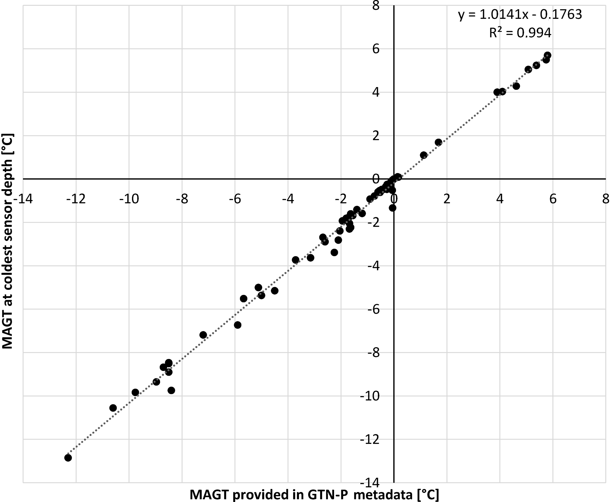
Figure 2Mean annual ground temperature (MAGT) derived from metadata (at or close to zero annual amplitude) versus derived MAGTc from the coldest sensor (for year of MAGT specified in the metadata) based on GTN-P borehole records. The dotted line represents the linear fit.
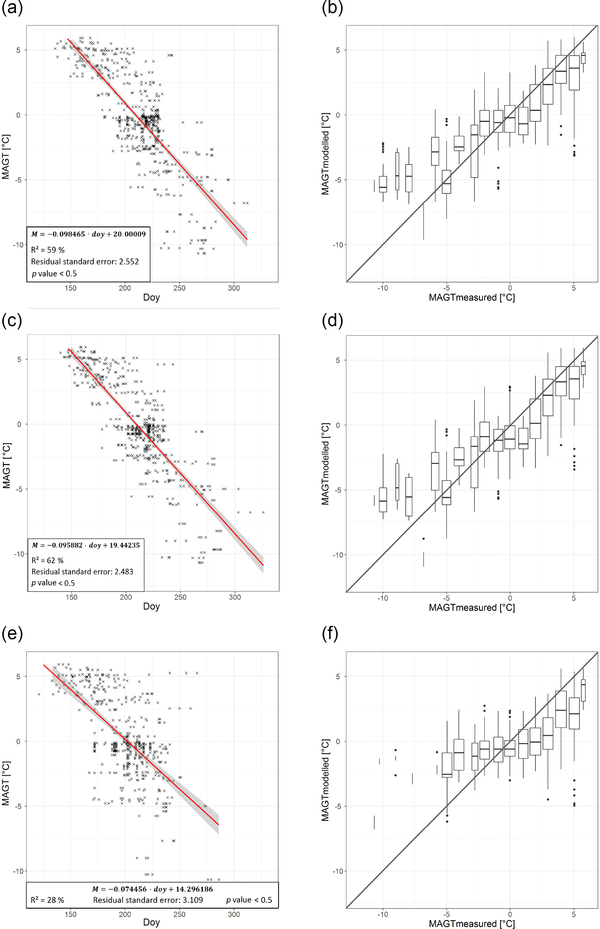
Figure 3(a, c, e) Comparison of number of frozen days (doy – days per year) from satellite records and mean annual ground temperature for GTN-P boreholes (at the depth of the coldest sensor, years 2010–2012). The red line represents the linear fit. (b, d, f) Box plots of modelled versus mean annual ground temperature from GTN-P boreholes (at the depth of the coldest sensor, years 2007/2008 and 2008/2009). (a, b) ASCAT excluding snow melt days, (c, d) ASCAT with snow melt days, and (e, f) SSM/I.
4.1 Evaluation of in situ MAGT at the coldest sensor depth
The 64 borehole locations had metadata suitable for the assessment. A total of 20 of the boreholes belong to the Vorkuta GTN-P site. R2 between MAGT from meta-records (GTN-P) and MAGTc is 0.994 (Fig. 2). The slope of the linear fit was close to 1 and the RMSE was 0.38 ∘C. Derived values tended to be colder by 0.2 ∘C on average. The coldest sensor depth and sensor to be used agreed in 58 (90 %) of the samples. Deviations of sensor depth occurred only for the Alaskan sites Bonanza Creek and Atmautluak as well as Arctic Bay (Nunavut Canada), Kursflaket 2 (Sweden), Ishim (Tyumen, Russia) and Kotkino (western Russia), however, with only little deviations in MAGT. Deviations were below 0.1 ∘C except for Bonanza Creek (−0.39 ∘C). MAGTc seems to also be valid as a substitute for MAGT at ZAA in non-permafrost regions based on the available records.
4.2 Potential mean annual ground temperature at the coldest sensor depth
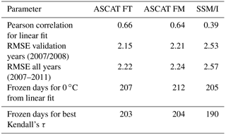
The Pearson correlation for the linear fit decreased slightly from 0.66 to 0.64 if snow melting days were included (Fig. 3 and Table 1). The same applied to the residual standard error (2.15 vs. 2.21) for the validation years. The slope of the linear fit also differed slightly between the two ASCAT data sets (Fig. 3). It was steeper in the case of exclusion of melting days as well as for SSM/I. The spread of in situ temperature values was higher for conditions below 0 ∘C than conditions above. This was similar for all data sets. The majority of MAGTc values (in a wide range of −10 to 5 ∘C) were found in the sector between 170 and 250 frozen days per year for ASCAT. The Pearson correlation in the case of SSM/I was lower with 0.39 and the RMSE was higher with 2.53 ∘C (Fig. 3). A difference of 11 frozen days of near-surface soil corresponded to 1 ∘C in the case of ASCAT FT.
Table 1Comparison between in situ mean annual ground temperature (MAGTc, at the coldest sensor depth) with number of frozen days per year from ASCAT (FT – excluding snow melt days; FM – including snow melt days) and SSM/I for 2007–2012.
Deviations in derived potential MAGTc between ASCAT and SSM/I occurred within and outside the continuous permafrost region (Fig. 4). Larger differences occurred over mountain ranges and lake-rich areas. Modelled MAGTc values based on SSM/I were mostly warmer in the continuous zone. The temperature difference between ASCAT (FT) and SSM/I exceeded 2 ∘C in the central Siberian transition zone, where SSM/I retrievals resulted in colder MAGTc than for ASCAT.
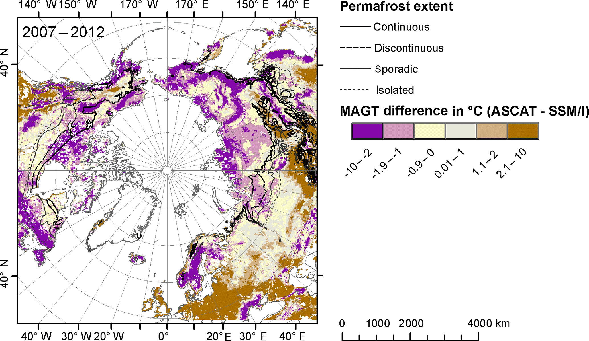
Figure 4Comparison of MAGTc (coldest sensor) in degrees Celsius of all years between Metop ASCAT (FT) and SSM/I for 2007–2012. Source of permafrost extent classes is Brown et al. (1997).
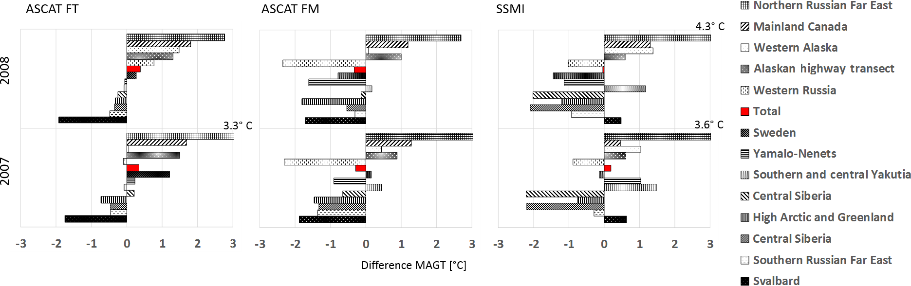
Figure 5Difference between modelled MAGTc and in situ MAGTc (coldest sensor) by region (see Fig. 1) in 2007/2008 and 2008/2009. FT – days identified as frozen without melting snow are used; FM – days with melting snow are considered to be frozen ground in ASCAT.
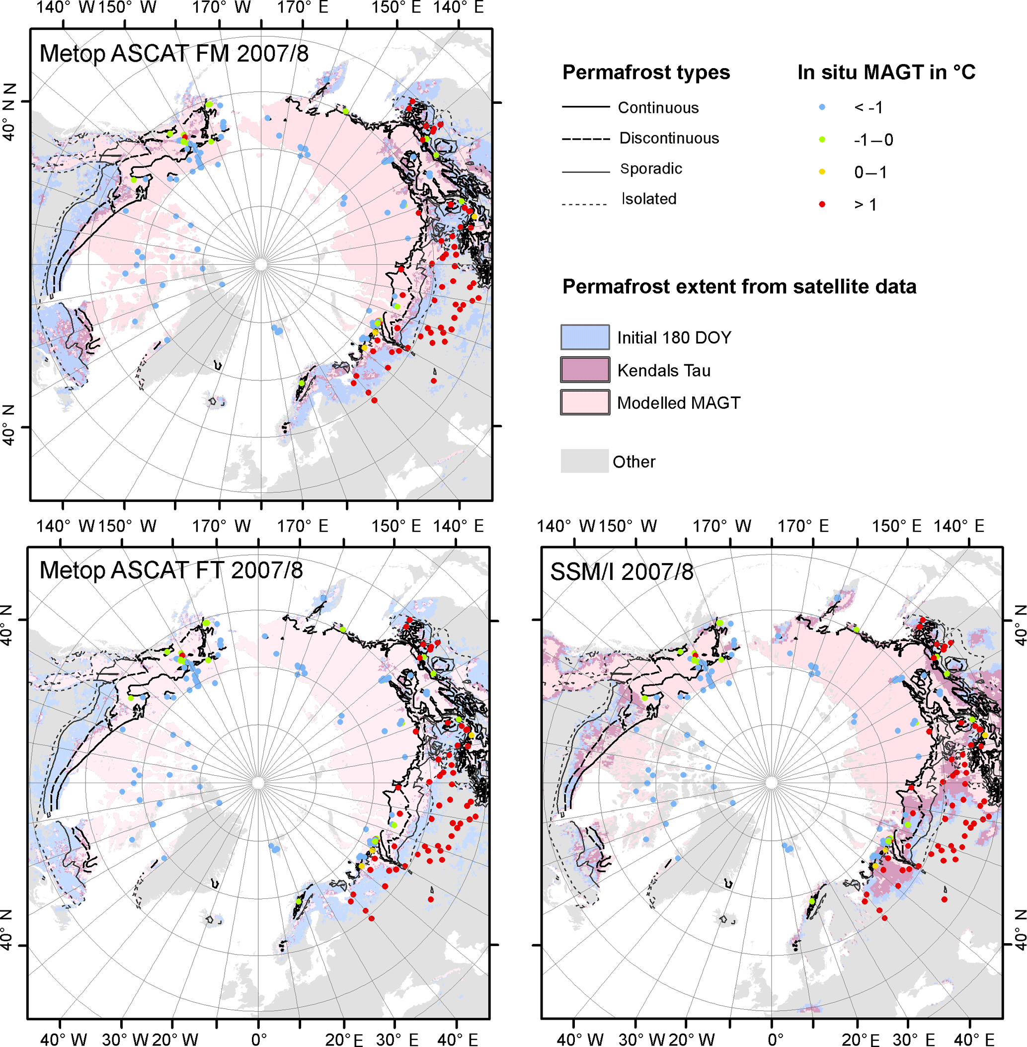
Figure 6Permafrost extent maps based on thresholds applied to frozen days per year (DOY) for ASCAT excluding melt days (FT), thresholds applied to frozen days per year (DOY) for ASCAT including melt days (FM), and thresholds applied to frozen days per year (DOY) for SSM/I. The initial threshold is 180 days. The value for the best Kendall's τ represents the best fit with borehole measurements. The highest threshold has been determined using an empirical model calibrated with borehole measurements. See also Table 1. All satellite results are based on 2007/2008–2008/2009 records. Source for permafrost extent classes is Brown et al. (1997).
4.2.1 Evaluation with in situ data with respect to region
The regionally averaged difference was mostly below 1 ∘C for all three products (Fig. 5). The deviations of ASCAT results from in situ records also differed for most regions between the two validation years. Large differences occurred specifically in western Russia and across Siberia for ASCAT FM as well as SSM/I. The exclusion of snow melting days reduced these differences. The deviations of the SSM/I product were largest in central Russia and the Yakutsk region. This was consistent with the patterns observed in comparison to the permafrost map (Fig. 6) and the deviations between the permafrost extent maps (Figs. 7 and 8).
The inclusion of days with melting snow reduced the deviations in the Yamalo-Nenets district, western Russia, and the Canadian High Arctic and Greenland (Fig. 5). The model result for ASCAT FM was about 2 ∘C colder than in the case of exclusion of melting snow. In contrast, MAGTc increased for Alaska. Median values were in general similar between inclusion and exclusion of melting snow (Fig. 9). All model results, ASCAT FT, FM and SSM/I, showed the highest deviations for the northern Russian Far East. Modelled temperatures were up to 7 ∘C too warm (median difference 3–5 ∘C). Most boreholes in the region are located in comparably cold permafrost.
4.2.2 Evaluation with in situ data with respect to environmental conditions
Deviations of MAGTc were larger at sites with a SWE larger than 150 mm (Fig. 11). Model results were colder than retrievals from the in situ records. This also applied to exclusion of the snow melting period. However, the exclusion reduced deviations in all medium SWE classes. Sites with a high SWE were mostly located in western Russia (Vorkuta region, Bolvansky) and western Siberia (Nadym region, Urengoy).
The regions identified as sporadic and isolated permafrost in Brown et al. (1997) showed comparably large deviations (Fig. 11). The isolated class did however only include five samples. The exclusion of snowmelt specifically reduced the deviations in the discontinuous zone. In the case of the ASCAT products, the average deviation was always below 1 ∘C in the continuous permafrost zone. The exclusion of melting snow clearly reduced deviations in the case of high ground ice content.
Figure 10 shows results for different land cover classes. Deviations are of an order of magnitude similar to that of the other parameters. They are highest for the SSM/I results. This applies specifically to landscapes which are shrub dominated and in proximity of water bodies. Only two samples were available in the burned area class. The model results were warmer in both cases. Sites which were contained in the water class were located in proximity to larger lakes or ocean.
Deviations seemed to be larger for sites with a certain SOC content (> 10 kg m−2 within the top metre; Fig. 12). Modelled MAGTc was on the order of 2 ∘C higher than derived from in situ data.
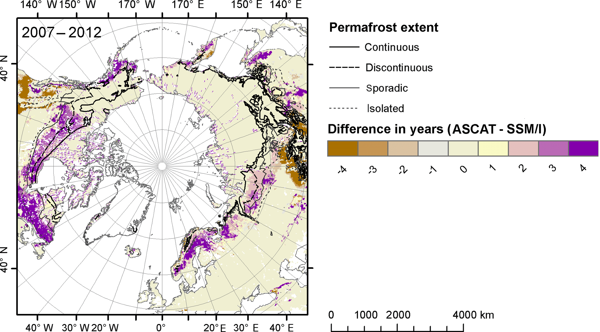
Figure 7Comparison of the total number of years classified as permafrost between Metop ASCAT and SSM/I for 2008–2012 based on the 180-day threshold method applied to all years (minimum of 2 consecutive years with at least 180 days frozen).
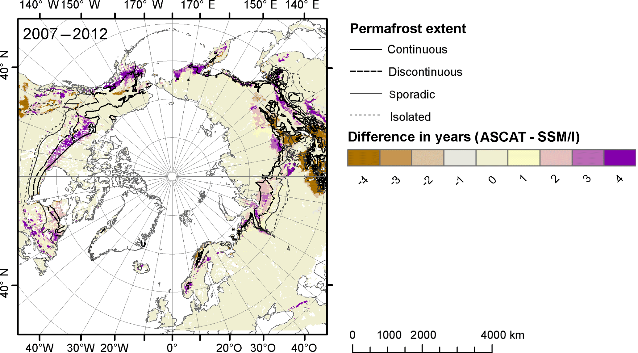
Figure 8Comparison of the total number of years classified as permafrost between Metop ASCAT (FT) and SSM/I for 2008–2012 based on the 0 ∘C temperature threshold method applied to all years (minimum of 2 consecutive years with below 0 ∘C). Source of permafrost extent classes is Brown et al. (1997).
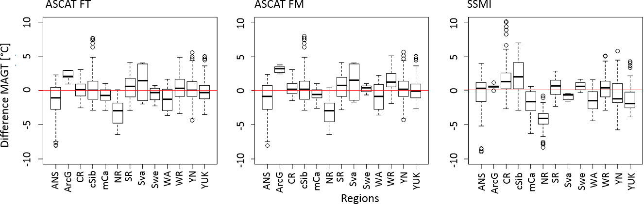
Figure 9Difference between in situ MAGTc (coldest sensor) and modelled MAGTc by region (see Fig. 1 for abbreviations and map) for all years. Only stations which overlap with records from all data sets are considered. FT – days identified as frozen without melting snow are used; FM – days with melting snow are considered to be frozen ground in ASCAT.
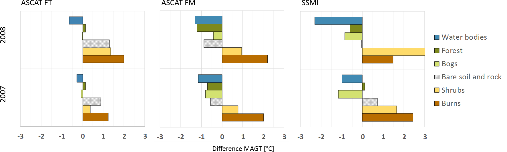
Figure 10Difference between modelled MAGTc and in situ MAGTc (coldest sensor) by land cover type (source is GLC2000, 2003) in 2007/2008 and 2008/2009. FT – days identified as frozen without melting snow are used; FM – days with melting snow are considered to be frozen ground in ASCAT. Note that the class “burns” contains only two samples in all cases (“Amboliha 4 07” and “Shimanovskaya” in the northern and southern Russian Far East, respectively).
4.3 Permafrost extent estimation
4.3.1 Threshold sensitivity analyses
The area mapped as permafrost with a frozen day threshold of 180 days for the period 2007–2011 differed regionally between the ASCAT and the SSM/I data sets (Fig. 7). The extent of areas where only ASCAT determined permafrost was about 4 times higher than for SSM/I. The latter largely occurred outside the expected permafrost region. Deviations in the transition zone were low for western Siberia but still present. The classification using SSM/I data resulted in a smaller permafrost extent for the Canadian Arctic compared to Brown et al. (1997). Most of the transition zone (including sporadic and isolated) in this region had more than 180 days frozen in the ASCAT data set. The Canadian High Arctic was also largely not covered by the SSM/I data set. ASCAT overestimated the permafrost extent in Scandinavia. In general, high-latitudinal lowland permafrost was overestimated with ASCAT, whereas the extent in more southern uplands and mountain regions was overestimated with SSM/I using the initial threshold.
Mapped permafrost extent varied for each threshold step across the different zones. The largest deviation in area extent for continuous permafrost occurred in the SSM/I result, with more than 2.5 million km2 lower values than in Brown et al. (1997) (more than 12 %, Table 2). Less than 1 million km2 (less than 5 % of total continuous permafrost area) was missed by ASCAT. This applied to thresholds between 180 and 200 frozen days (excluding snow melt days). Matching extent was lowest for 200 days in the case of inclusion of snow melt days. ASCAT mapped more permafrost outside the boundaries of Brown et al. (1997) than SSM/I in the case of a 180-day threshold but agreed better than SSM/I for discontinuous and isolated permafrost area. This resulted in lower percentage agreement of the SSM/I product for the total permafrost extent (Table 3). The false permafrost detection by ASCAT was outweighted by a significantly higher detection performance for the total extent. There was also more year-to-year variability in the results from the analysis using SSM/I data than using ASCAT.
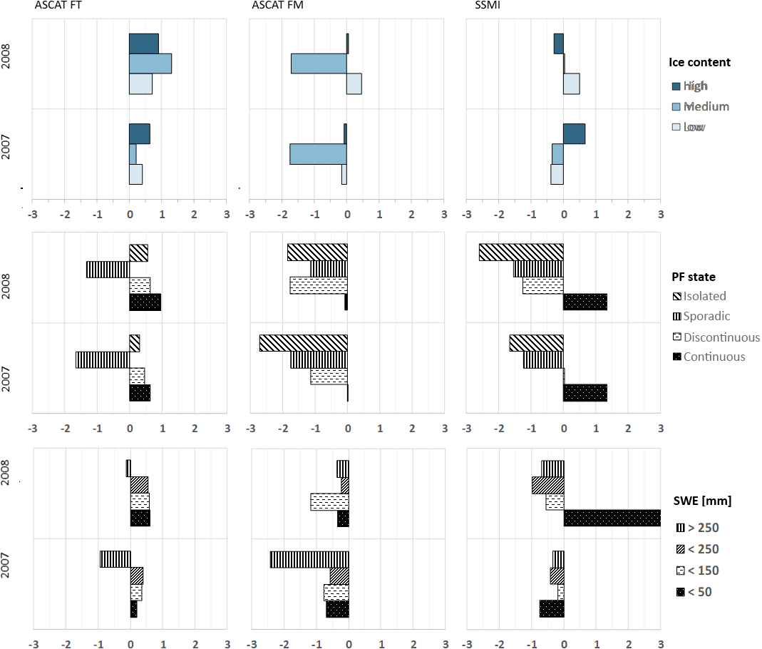
Figure 11Difference between modelled MAGTc and in situ MAGTc (coldest sensor) by permafrost zone and ice content (source is Brown et al., 1997), and snow water equivalent (SWE; source is GlobSnow) categories in 2007/2008 and 2008/2009. FT – days identified as frozen without melting snow are used; FM – days with melting snow are considered to be frozen ground in ASCAT. Note that the class with a SWE < 50 mm contains only two samples in the case of SSM/I for 2008 (“Tiksi stone ridge” and “Dionisiy-111(2)” in the northern Russian Far East).
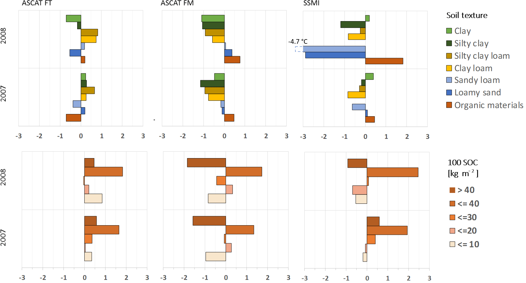
Figure 12Difference between modelled MAGTc and in situ MAGTc (coldest sensor) by soil texture (source is Fischer et al., 2008) and soil organic carbon content within the top 100 cm (100SOC; source is Hugelius et al., 2013, 2014) in 2007/2008 and 2008/2009. FT – days identified as frozen without melting snow are used; FM – days with melting snow are considered to be frozen ground in ASCAT.
4.3.2 Determination of optimal threshold with Kendall's τ test and in situ measurements
The comparison of the satellite records with in situ data demonstrated differences between the data sets. For the ASCAT data sets the best τ was found to coincide with 204 (FM) and 203 (FT) frozen days per year (Table 1), whereas for the SSM/I, 190 frozen days per year showed the highest τ with a steep gradient before and after the peak (Fig. 13).
With the frozen days per year threshold of 180 days, the algorithm tended to overestimate the number of negative MAGTc values, while the threshold found by the Kendall's τ led to an underestimation of negative MAGTc values below the threshold (Table 4). It was highest for exclusion of snow melting days. Conversely, the ASCAT results showed nearly no negative MAGTc below the threshold of 180. The thresholds delineated by the best correlation coefficient (Kendall's τ) indicated for all data sets a better performance regarding positive MAGTc in areas below the threshold. However, the higher thresholds also led to more negative MAGTc in these areas. For the SSM/I 75 % of MAGTc temperatures could be correctly allocated with both thresholds. The ASCAT results showed a higher accuracy with more than 80 % correctly assigned values.
ASCAT and SSM/I maps derived with the initial threshold of 180 days mostly agreed in the continuous permafrost zones over the four analysis periods (Fig. 7). ASCAT overestimated permafrost extent in North America, Scandinavia and western Siberia. SSM/I overestimated specifically in southern central Siberia.
4.3.3 Classification of modelled MAGT for the coldest sensor depth
The classification of the derived MAGTc data set provided different results than the other methods for permafrost extent determination. The frozen days per year for intersection of the derived linear function at 0 ∘C corresponded to a higher number of frozen days in all cases (Table 1).
The FT and FM methods differed more for the year 2007 than for 2008 (Fig. 14 and Table 5). The SSM/I extent missed a large proportion of continuous permafrost and mapped additional area as permafrost (more pronounced in 2007, Table 5), similar to the initial threshold-based comparison to the permafrost extent map (Table 2).
The number of years with MAGTc below 0 ∘C were similar between ASCAT (FT) and SSM/I in the lowland continuous permafrost zones (Fig. 7). Deviations were high in transition zones, especially southern central Siberia, with a similar spatial pattern as already observed in the case of initial threshold comparison (Fig. 6). The results deviated for all four periods in this region, meaning that SSM/I always remained below a MAGTc below 0 ∘C, and ASCAT was not below a MAGTc below 0 ∘C in any of the periods.
4.3.4 Comparison among permafrost extent maps
The results from all three tested methods for potential permafrost determination (half-year threshold, best Kendall's τ and from modelled MAGTc) are shown in Fig. 6. The largest spatial differences between included and excluded melting days occurred in the same regions (northeastern Canada and Scandinavia), which showed the largest differences between the ASCAT and SSM/I 180-day threshold maps. An additional region of disagreement was Yakutsk. The inclusion of snow melting days here led to a reduction of permafrost extent, which was contradictory to most other regions.
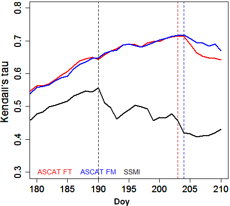
Figure 13Curves of correlation coefficient (Kendall's τ) between 180 and 210 days per year (doy) frozen from satellite products and positive or negative MAGTc at the depth of the coldest sensor from borehole data. FT – days identified as frozen without melting snow are used; FM – days with melting snow are considered to be frozen ground with Metop ASCAT.
Table 2Permafrost extent comparison of satellite data results from Metop ASCAT based on modified thresholds (180, 190, 200 and 210 days) with permafrost extent classes from Brown et al. (1997). Covered area is provided in square kilometres within each class. FT – days identified as frozen without melting snow are used; FM – days with melting snow are considered to be frozen ground with Metop ASCAT. SSM/I classification results based on 180 days are included for comparison.
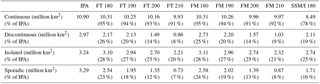
Table 3Comparison of satellite data results based on a 180-day threshold with permafrost extent from Brown et al. (1997). Covered area in percent inside and outside permafrost regions is provided. FT – days identified as frozen without melting snow are used; FM – days with melting snow are considered to be frozen ground with Metop ASCAT.
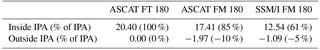
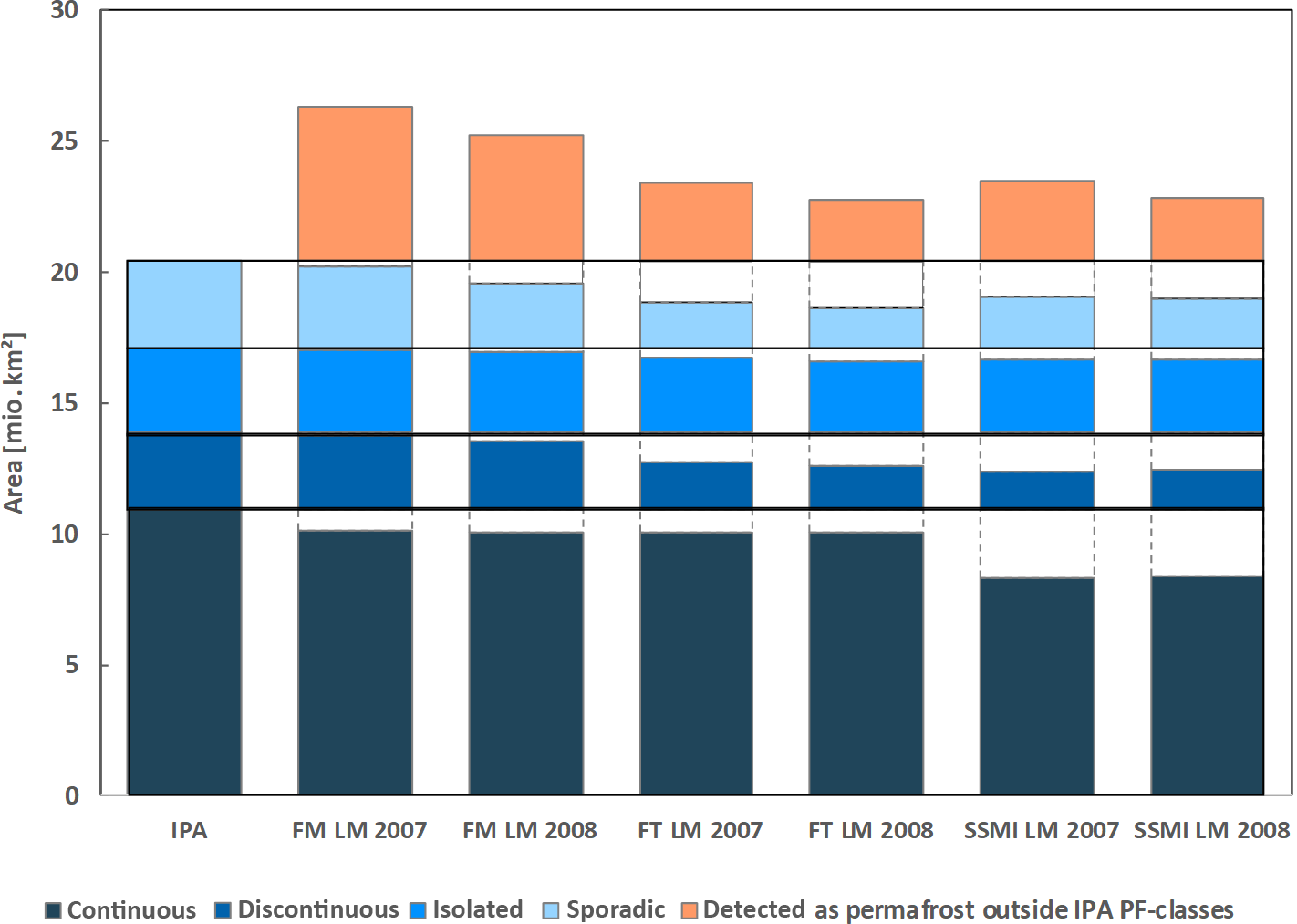
Figure 14Permafrost extent comparison of satellite data results based on modelled ground temperatures (LM – linear model) with permafrost classes from Brown et al. (1997). Covered area in square kilometres within and outside each class. FT – days identified as frozen with ASCAT; FM – days with melting snow are considered to be frozen ground with ASCAT.
Table 4Comparison matrix between in situ mean annual ground temperature (MAGTc, at the coldest sensor depth) classes (below or above zero ∘C) and classified number of frozen days per year from ASCAT (FT – excluding snow melt days; FM – including snow melt days) and SSM/I for 2007–2012. Both the initial 180 days per year (DOY) threshold and the optimal threshold based on the best Kendall's τ are assessed. Values represent numbers of sites for multiple years. Rows indicating false classifications are in italic.
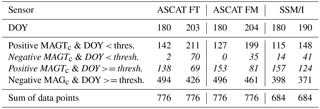
Table 5Comparison of satellite data results based on modelled ground temperatures with permafrost extent from Brown et al. (1997). Covered area in percent inside and outside permafrost regions. FT – days identified as frozen without melting snow are used; FM – days with melting snow are considered to be frozen ground; LM – model results.
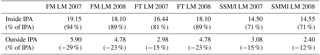
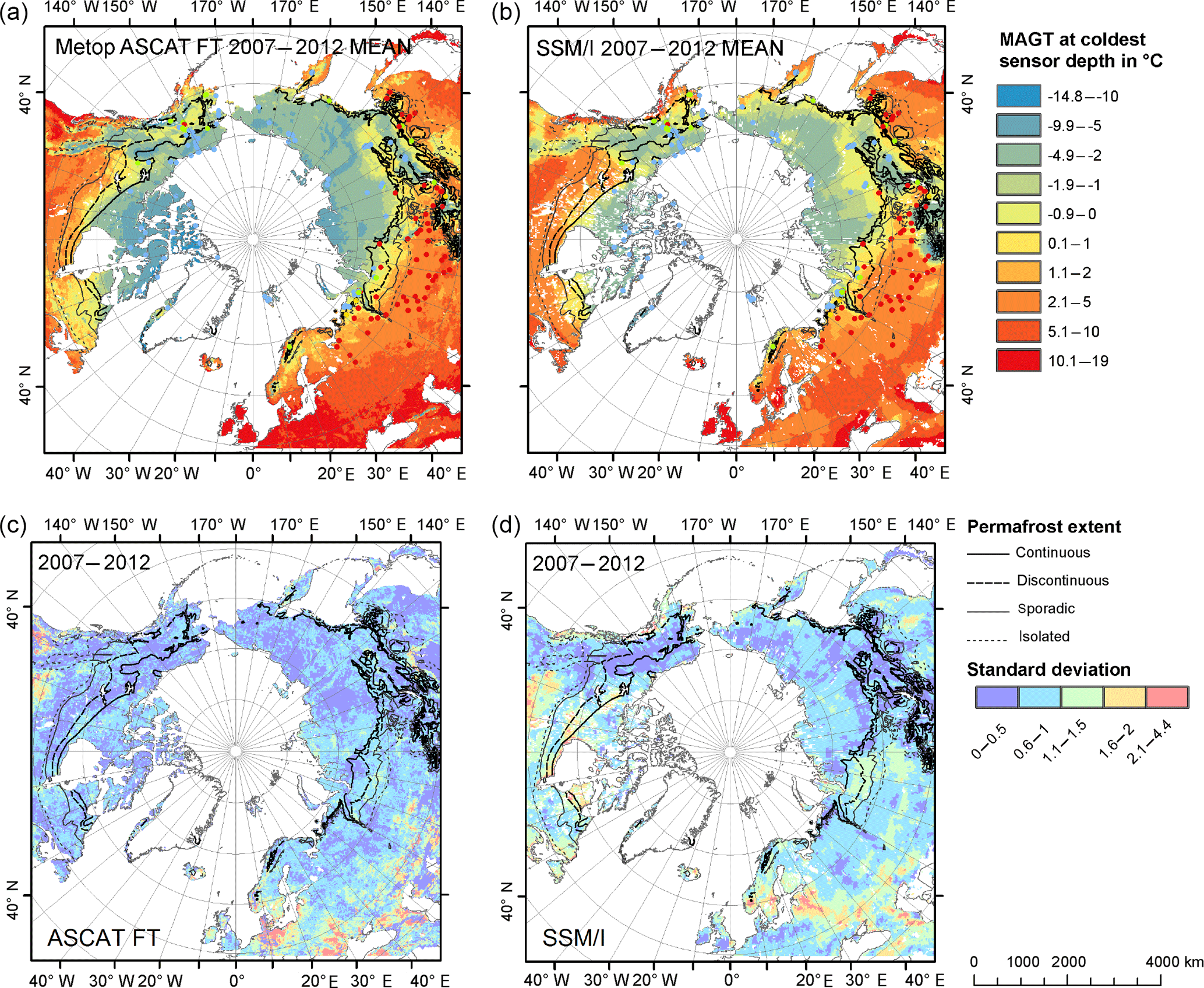
Figure 15Maps of modelled mean annual ground temperature (a, b) and standard deviation of modelled MAGTc (c, d) for ASCAT excluding melt days (FT; a, c) and SSM/I (b, d) based on all analysed years. Source for permafrost extent classes is Brown et al. (1997).
The modelled extent and best Kendall's τ threshold results included the discontinuous permafrost zone in North America for ASCAT (Fig. 6). The exclusion of melting snow had a large impact over Scandinavia. It led to results which are more similar to the map of Brown et al. (1997). It was also one of the regions with extensive snowmelt detected by ASCAT (Fig. A1). Patterns of continuous permafrost boundaries in central Asia (e.g. region around lake Baikal) were better represented in the ASCAT maps than in the SSM/I retrievals.
Variation in potential MAGTc from year to year was much larger for SSM/I. Standard deviation was comparably high for the transition zone in western Siberia and also the Canadian Arctic (Fig. 15). This pattern agreed with results obtained with the initial threshold in comparison to Brown et al. (1997) (see Sect. 4.3).
5.1 General issues
The performance of the empirical model for MAGTc (Table 1) was partially lower than what can be achieved with the more complex temperature at the top of permafrost (TTOP) model (Westermann et al., 2015), which considers terrain, snow, land cover and land surface temperature measurements from satellite data. Westermann et al. (2015) reported a model accuracy of 2.5 ∘C for MAGT. Permafrost temperatures also do not always represent current climate conditions (Lachembruch and Marshall, 1986). This may regionally impact the comparability of the borehole records with surface observations. Estimates of permafrost temperatures as well as extent therefore provide a potential distribution only. Results may however support the identification of regions where permafrost extent maps, including continuity classes, need to be treated with care. This includes western and central Siberia. The overall performance of permafrost extent mapping using number of frozen days is limited but reveals regional patterns in uncertainties. The extent of permafrost estimated with the initial threshold is on the order of the actual extent. The error of commission is, however, relatively large. This problem can be tackled by adjustment of the threshold and use of different types of satellite acquisitions (ASCAT versus SSM/I).
The MAGT from boreholes was calculated from the coldest sensor below 1 m. The depth of these sensors varied from borehole to borehole, which may impact the empirical model representativity. A high number of sites was however chosen for calibration, which may weaken the impact. The evaluation results with MAGT (expected to be at or close to ZAA) in the meta-records for 24 % of the sites support the assumption that the sensor at the coldest depth can be used for approximation. Uncertainties introduced by variable sensor spacing can, however, not be addressed with the available data.
The in all cases (ASCAT and SSM/I, for all permafrost retrieval methods) higher accounts of the number of frozen days than the previously suggested half-year threshold agrees with field observations by Luoto et al. (2004), who estimated a minimum number of 200 days for permafrost formation for Scandinavia. A total of 200 days corresponds to approximately 0.5 ∘C modelled MAGTc in the case of ASCAT FT. Considering local factors such as water-saturated peat and organic layer as well as uncertainties in the retrieval (difference to actual mean temperature), this might still be sufficient for permafrost formation. Variations in topography within the footprint also lead to local deviations from days to weeks (Bergstedt and Bartsch, 2017). We therefore suggest the consideration of temperature buffers when such data are applied. Boreholes with in situ MAGTc below 0 ∘C located in these buffer zones may represent sites at which local factors are important. In addition, the role of past climate conditions in present ground temperatures as well as location-specific soil and snow properties need to be considered (see Sect. 5.4).
The classes in Brown et al. (1997) correspond to the area fraction of permanently frozen ground. In the case of the isolated permafrost class it can be assumed that at least 10 % of ground area is below 0 ∘C, but the actual mean temperature for a region in these areas (as represented by an ASCAT or SSM/I cell) can be below or above 0 ∘C depending on local parameters such as topography and soil properties which impact thermal conductivity. The latter especially plays a role in occurrence of permafrost in the transition zone. Data sets of higher spatial resolution would be required. Relevant measurements from microwave data are only available from active systems due to technical constraints. Synthetic aperture radar (SAR) instruments could be used in the case of sufficient sampling intervals (Park et al., 2011b). Current systems and acquisition plans do not however provide sufficient temporal and spatial sampling (Bartsch et al., 2016a).
5.2 Regional issues
A threshold higher than the previously suggested half year leads to better performance of ASCAT than for SSM/I for permafrost extent retrieval, especially over Scandinavia, western Russia and southern Russian Far East (Fig. 6; region overview in Fig. 1). ASCAT better captures the regional patterns of Brown et al. (1997) with the exception of Scandinavia. The actual temperature amplitude (freezing and thawing degree days) may need to be considered in this region. The longer snow melt period (Fig. A1) also indicates a certain amount of snow which may lead to decoupling of air and ground temperatures.
The highest density of boreholes with available data is in the Vorkuta region in western Russia. This region shows the largest sensitivity to inclusion–exclusion of snow melting days (Fig. 5). Here, the ASCAT MAGTc results differ by more than 2 ∘C (lower temperature). This might have an impact on the average deviation derived from all the borehole records. It is likely larger for the ASCAT FM result than calculated as most other regions show better agreement.
The validation results in the regions central Russia and central Siberia differ from those of the other areas. SSM/I results suggest between 1 and 2 ∘C lower regionally averaged MAGTc values (Figs. 5 and 9). The majority of boreholes located in these regions show MAGTc higher than 0 ∘C (Fig. 1). This deviation therefore impacts the permafrost boundary retrieval based on freeze–thaw records from SSM/I. These regions are characterized by a longer-than-average period of diurnal thaw and refreeze cycling during spring melt (Bartsch, 2010; Bartsch et al., 2007). Acquisition timing may therefore play a role in the determination of the length of the frozen period.
The Greenland and Svalbard sites are expected to have the highest variations due to the mixture of glaciers, land area and ocean within the ASCAT as well as SSM/I pixels. There is actually no coverage of the Greenland and several Canadian High Arctic sites in the SSM/I records.
5.3 Performance differences between ASCAT and SSM/I
Results suggest that SSM/I freeze–thaw records are less suitable to derive actual MAGTc values below 0 ∘C compared to ASCAT (Fig. 4). The thresholds obtained for SSM/I are considerably lower than for ASCAT, what might be the result of the different wavelength, the sensing technique (passive or active), overpass timing and classification methods used to create these data sets. The considerably lower number of frozen days in regions with low MAGTc might be the result of the retrieval method (treatment regarding acquisition timing) and sensitivity to soil state changes. The instruments also differ in wavelength apart from the fact that one is active and the other passive. ASCAT uses C band with about 5.7 cm and the SSM/I channel used by Park et al. (2016) uses about 0.8 cm. This results in different signal interactions with objects on the Earth's surface including snow and vegetation. It can be expected that the C-band signal is less sensitive to interactions, although present. The latter issue could be addressed by L-band missions with an even lower frequency than ASCAT such as the SMOS (Soil Moisture and Ocean Salinity) mission or SMAP (Soil Moisture Active Passive). In general, the role of acquisition timing and sampling rate needs to be investigated in more detail for permafrost-related applications for ASCAT as well as SSM/I.
The lower performance of SSM/I might also be attributed to the fact that it has an even larger footprint (although gridded to 25 km) than ASCAT. The validation results are therefore not fully comparable between the sensors for the entire Arctic, only on a regional level. This may also affect the calibration since the number of available samples is lower for SSM/I. It especially affects colder sites (Fig. 3). In general, fewer areas are masked in the ASCAT product. This especially applies to lake-rich regions (Fig. 6). Findings of Bergstedt and Bartsch (2017) suggest an offset of the state change in the resolution cell due to lakes. This may lead to lower accuracy in these regions.
5.4 The role of environmental conditions
The amount of snow seems to play the most important role for the applicability of the frozen day approach. One may expect warmer modelled MAGTc than in situ values in transition zones due to the fact that boreholes in transition zones often represent isolated patches of permafrost. However, the opposite is the case (Fig. 11). This may relate to the importance of the insulation effect of snow cover in these regions, e.g. as known for Scandinavia (Luoto et al., 2004).
The number of snow melting days is in general highly variable in the Arctic (Bartsch, 2010) but the melting period is comparably short (Zhang et al., 2005). Snowmelt is expected to delay the soil surface warming due to latent heat and therefore cools the soils (Zhang et al., 2005). Latent heat released due to refreezing of meltwater may have a warming effect after a few days (Dingman et al., 1980). Dingman et al. (1980) also report start of soil thaw before the end of snowmelt at Utqiaġvik (formerly Barrow). The overall impact of snowmelt is expected to be dependent on local conditions (Zhang et al., 2005). Our results suggest that there is a warming effect with an impact on MAGTc. Days with melting snow should therefore be treated as unfrozen. This leads to higher MAGTc (on average 1 ∘C for considered borehole locations) and better agreement with in situ measurements. Exclusion of the snowmelt period is also consistent with calculation of thawing and freezing degree days from air temperature data. The snowmelt period does also count as unfrozen in this case.
Snow melting days are, however, not mapped for all grid points in the case of the ASCAT data set (Fig. A1). This may depend on snow depth as well as acquisition timing. The coverage pattern is irregular across the Arctic with a mix of morning and evening (ascending and descending orbits) measurements (Bergstedt and Bartsch, 2017). Usually only evening measurements capture the melt as diurnal freeze and thaw cycles are common (Bartsch et al., 2007). The differentiation between frozen and melting days may however be valid in regions with prolonged melt and high SWE. Areas with melting snow in the ASCAT data set are common in the high Arctic, in areas with low MAGTc (Fig. A1) and in areas in the transition zone (such as Scandinavia). This pattern differs from the length of the snowmelt period detected with SeaWinds QuikSCAT, a Ku-band scatterometer (Bartsch, 2010), which provides several measurements per day. The number of days with snow melt are much lower in the C-band than in the Ku-band product. This could be attributed to the lower sensitivity of the C band to melting processes and the limited temporal sampling. In addition, the QuikSCAT results reported by Bartsch (2010) represent periods of freezing and thawing which can contain breaks (with frozen conditions) of up to 10 days.
Land cover (Fig. 10) plays a role when comparing performance of SSM/I versus ASCAT. Boreholes, which fall into the water class according to GLC2000, are located close to coasts. The coarser-resolution SSM/I data sets are more affected here than ASCAT. Deviations are therefore larger for SSM/I. Modelled results are on average warmer in all cases for the class “shrubs”. This mostly represents the tundra biome and is also the largest sample. It overlaps with continuous permafrost, which shows a similar bias (Fig. 11). The difference is larger in the case of SSM/I, which might relate to the fact that the variation in below-zero MAGTc is not well reflected in the SSM/I-derived number of frozen days, and also fewer samples have been available for colder sites due to masking (Fig. 3).
An influence of soil organic carbon on deviations between the modelled temperature and in situ measurements cannot be clearly exemplified (Fig. 12). This might be partially influenced by spatial inconsistencies and the nature of the used database (Bartsch et al., 2016c). SOC is represented by areal averages only, but it is the most detailed data set available to date. The tendency for warmer modelled temperature in the case of sites with more than 10 kg m−2 of SOC agrees, however, with the expected effect of organic soils on ground thermal regime (Smith and Riseborough, 2002). Sites with sandy loam and loamy sand seem to differ between ASCAT and SSM/I results. They represent different regions across central Siberia and western Russia, but the sample size is much smaller than for the other categories. This, however, agrees with the observed regional patterns for differences between the methods.
Conventional approaches for spatially continuous mapping of permafrost temperatures require gap filling or spatial interpolation. This applies to the use of in situ temperature measurements as well as to satellite-derived land surface temperature (thermal and passive microwave). The direct comparison of microwave-satellite-derived surface status (frozen–unfrozen), rather than actual temperatures, to borehole temperatures revealed the potential of such information for ground temperature estimation. C-band backscatter-based records performed better than surface status derived from passive microwave brightness temperature. The relationship between MAGT at the coldest sensor depth with SSM/I-derived surface status is comparably weak, especially for lower temperatures. ASCAT can capture variations over the full MAGT range investigated. The C-band scatterometer record can therefore provide a purely observational estimate of MAGT. This refers to temperatures at the coldest sensor depth and not necessarily zero annual temperature range, due to limitations of the in situ data records. It could be, however, shown that MAGT at the coldest sensor depth can be used as a substitute for actual MAGT for validation and calibration purposes.
Our study also points to the role of snow status (dry or melting) in the temperature of the soil beneath and subsequent impact on MAGTc. A linear empirical model performed best when days with melting snow were excluded. The overall RMSE was 2.2 ∘C with ASCAT but the modelled temperature deviated on average by less than 1 ∘C in footprints without glaciers and a mix of land and water. Especially regions with large variations in frozen days among the years and/or among the three different analyses (ASCAT with snow melting days and without, the SSM/I records) need to be further investigated with respect to the representativity of the borehole records and derived temperatures (e.g. western Siberia). They mostly correspond to the permafrost transition zones. The validity of the coarse-resolution microwave satellite records for the point locations needs to be confirmed by using higher-spatial-resolution synthetic aperture radar (SAR) records, for example. More detailed analyses of the impact of melting snow conditions is also required in order to clarify underlying processes. Results also exemplify the role of organic material in thermal conductivity which is not accounted for with the application of a global empirical relationship.
In addition, the suitability of surface state information from satellite data for permafrost extent estimation could be confirmed, but differences among the tested methods and data sets were also evident. Agreement was high within the continuous permafrost zone (as defined in Brown et al., 1997), except for mountain ranges. Deviations in transition areas were largest in central Siberia and areas with high snow depth. This underlines the importance of snow and suggests that advanced models should be applied in the areas of the mountain ranges in central Asia, including southern and central Yakutia and Mongolia. These regional differences should be considered in interpretation of especially long-term trends.
The average annual sums of frozen and snow melting days derived from Metop ASCAT are available via the ESA DUE GlobPermafrost project WebGIS and catalogue (http://maps.awi.de/map/map.html?cu=globpermafrost_arctic) (AWI, 2018). The average number of unfrozen days from ASCAT is published in Bartsch et al. (2016b).

Figure A1Average number of snow melting days per year from Metop ASCAT for 2007–2013 derived from Paulik et al. (2014).
CK has performed all satellite data analyses and contributed to the preparation of figures. The concept of the paper was jointly developed by CK and AB. HB supported the in situ data evaluation. AB wrote the majority of the paper. CK contributed to the writing of the in situ, methods and results sections, HB to the satellite data description and discussion.
The authors declare no conflict of interest.
This article is part of the special issue “Changing Permafrost in the Arctic and its Global Effects in the 21st Century (PAGE21) (BG/ESSD/GMD/TC inter-journal SI)”. It is not associated with a conference.
This work was supported by the Austrian Science Fund (Fonds zur Förderung
der wissenschaftlichen Forschung, FWF) under grant (I 1401) (Joint
Russian–Austrian project COLD-Yamal), grant (DK W1237-N23) (Doctoral College
GIScience) and the European Space Agency project DUE GlobPermafrost
(contract number 4000116196/15/I-NB).
Edited
by: Julia Boike
Reviewed by: three anonymous referees
André, C., Ottlé, C., Royer, A., and Maignan, F.: Land surface temperature retrieval over circumpolar Arctic using SSM/I–SSMIS and MODIS data, Remote Sens. Environ., 162, 1–10, https://doi.org/10.1016/j.rse.2015.01.028, 2015. a
AWI: ESA DUE GlobPermafrost project webgis and catalogue, Alfred-Wegener-Institut Helmholtz-Zentrum für Polar- und Meeresforschung, available at: http://maps.awi.de/map/map.html?cu=globpermafrost_arctic, last access: 6 March 2018. a
Bartholomé, E. and Belward, A. S.: GLC2000: a new approach to global land cover mapping from Earth observation data, Int. J. Remote Sens., 26, 1959–1977, https://doi.org/10.1080/01431160412331291297, 2005. a
Bartsch, A.: Ten Years of SeaWinds on QuikSCAT for Snow Applications, Remote Sens., 2, 1142–1156, https://doi.org/10.3390/rs2041142, 2010. a, b, c, d
Bartsch, A. and Seifert, F. M.: The ESA DUE Permafrost project – A service for high latitude research, Int. Geosci. Remote Se., 5222–5225, https://doi.org/10.1109/IGARSS.2012.6352432, 2012. a
Bartsch, A., Kidd, R. A., Wagner, W., and Bartalis, Z.: Temporal and Spatial Variability of the Beginning and End of Daily Spring Freeze/Thaw Cycles Derived from Scatterometer Data, Remote Sens. Environ., 106, 360–374, https://doi.org/10.1016/j.rse.2006.09.004, 2007. a, b, c
Bartsch, A., Höfler, A., Kroisleitner, C., and Trofaier, A. M.: Land Cover Mapping in Northern High Latitude Permafrost Regions with Satellite Data: Achievements and Remaining Challenges, Remote Sens., 8, 979, https://doi.org/10.3390/rs8120979, 2016a. a
Bartsch, A., Kroisleitner, C., and Heim, B.: Circumpolar Landscape Units, links to GeoTIFFs, Pangaea, https://doi.org/10.1594/PANGAEA.864508, 2016b. a, b
Bartsch, A., Widhalm, B., Kuhry, P., Hugelius, G., Palmtag, J., and Siewert, M. B.: Can C-band synthetic aperture radar be used to estimate soil organic carbon storage in tundra?, Biogeosciences, 13, 5453–5470, https://doi.org/10.5194/bg-13-5453-2016, 2016c. a
Bergstedt, H. and Bartsch, A.: Surface State across Scales; Temporal and SpatialPatterns in Land Surface Freeze/Thaw Dynamics, Geosciences, 7, 65, https://doi.org/10.3390/geosciences7030065, 2017. a, b, c
Biskaborn, B. K., Lanckman, J.-P., Lantuit, H., Elger, K., Streletskiy, D. A., Cable, W. L., and Romanovsky, V. E.: The new database of the Global Terrestrial Network for Permafrost (GTN-P), Earth Syst. Sci. Data, 7, 245–259, https://doi.org/10.5194/essd-7-245-2015, 2015. a, b
Bodri, L. and Cermak, V.: Borehole Climatology: a new method how to reconstruct climate, Elsevier Science, 1st edn., 2007. a
Brown, J., Ferrians, Jr., O., Heginbottom, J., and Melnikov, E.: Circum-Arctic map of permafrost and ground-ice conditions, USGS Numbered Series no. 45, U.S. Geological Survey, 1997. a, b, c, d, e, f, g, h, i, j, k, l, m, n, o, p, q, r, s, t, u, v, w, x
Cheng, G. and Wu, T.: Responses of permafrost to climate change and their environmental significance, Qinghai-Tibet Plateau, J. Geophys. Res.-Earth, 112, F02S03, https://doi.org/10.1029/2006JF000631, 2007. a
Dingman, S., Barry, R., Weller, G., C.Benson, LeDrew, E., and Goodwin, C.: Climate, Snow Cover, Microclimate, and Hydrology, in: An Arctic Ecosystem: the Coastal Tundra at Barrow, edited by: Brown, J., Miller, P., and Bunnell, F., Hutchinson and Ross, Stroudsburg, PA, chap. 2, 30–65, 1980. a, b
Dobinski, W.: Permafrost, Earth-Sci. Rev., 108, 158–169, https://doi.org/10.1016/j.earscirev.2011.06.007, 2011. a
Figa-Saldaña, J., Wilson, J., Attema, E., Gelsthorpe, R., Drinkwater, M., and Stoffelen, A.: The advanced scatterometer (ASCAT) on the meteorological operational (MetOp) platform: A follow on for European wind scatterometers, Can. J. Remote Sens., 28, 404–412, https://doi.org/10.5589/m02-035, 2002. a
Fischer, G., Nachtergaele, F., Prieler, S., van Velthuizen, H., Verelst, L., and Wiberg, D.: Global Agro-ecological Zones Assessment for Agriculture (GAEZ 2008), IIASA, Laxenburg, Austria and FAO, Rome, Italy, available at: http://www.gaez.iiasa.ac.at/ (last access: 6 October 2017) 2008. a, b
GLC2000: The Global Land Cover Map for the Year 2000, European Commission Joint Research Centre, available at: http://www-gem.jrc.it/glc2000 (last access: 12 January 2017), 2003. a, b
GlobSnow: Global Snow Monitoring for Climate Research, available at: http://www.globsnow.info (last access: 12 January 2017), 2018. a, b
Gruber, S.: Derivation and analysis of a high-resolution estimate of global permafrost zonation, The Cryosphere, 6, 221–233, https://doi.org/10.5194/tc-6-221-2012, 2012. a
GTN-P: Global Terrestrial Network for Permafrost Database: Permafrost Temperature Data (TSP Thermal State of Permafrost), available at: https://gtnp.arcticportal.org/, last access: 28 December 2016. a
Harris, S. A.: Distribution of zonal permafrost landforms with freezing and thawing indices, Erdkunde, 35, 81–90, https://doi.org/10.3112/erdkunde.1981.02.01, 1981. a
Hayes, D. J., Kicklighter, D. W., McGuire, A. D., Chen, M., Zhuang, Q., Yuan, F., Melillo, J. M., and Wullschleger, S. D.: The impacts of recent permafrost thaw on land–atmosphere greenhouse gas exchange, Environ. Res. Lett., 9, 045005, https://doi.org/10.1088/1748-9326/9/4/045005, 2014. a
Hollinger, J. P., Peirce, J. L., and Poe, G. A.: SSM/I instrument evaluation, IEEE T. Geosci. Remote, 28, 781–790, https://doi.org/10.1109/36.58964, 1990. a
Hugelius, G., Tarnocai, C., Broll, G., Canadell, J. G., Kuhry, P., and Swanson, D. K.: The Northern Circumpolar Soil Carbon Database: spatially distributed datasets of soil coverage and soil carbon storage in the northern permafrost regions, Earth Syst. Sci. Data, 5, 3–13, https://doi.org/10.5194/essd-5-3-2013, 2013. a, b
Hugelius, G., Strauss, J., Zubrzycki, S., Harden, J. W., Schuur, E. A. G., Ping, C.-L., Schirrmeister, L., Grosse, G., Michaelson, G. J., Koven, C. D., O'Donnell, J. A., Elberling, B., Mishra, U., Camill, P., Yu, Z., Palmtag, J., and Kuhry, P.: Estimated stocks of circumpolar permafrost carbon with quantified uncertainty ranges and identified data gaps, Biogeosciences, 11, 6573–6593, https://doi.org/10.5194/bg-11-6573-2014, 2014. a, b
Kim, Y., Kimball, J. S., Zhang, K., and McDonald, K. C.: Satellite detection of increasing Northern Hemisphere non-frozen seasons from 1979 to 2008: Implications for regional vegetation growth, Remote Sens. Environ., 121, 472–487, https://doi.org/10.1016/j.rse.2012.02.014, 2012. a
Kim, Y., Kimball, J. S., Glassy, J., and McDonald, K. C.: MEaSUREs Global Record of Daily Landscape Freeze/Thaw Status, Version 3, https://doi.org/10.5067/MEASURES/CRYOSPHERE/nsidc-0477.003, 2014. a, b
Lachembruch, A. H. and Marshall, B. V.: Changing climate: geothermal evidence from permafrost in the Alaskan Arctic, Science, 234, 689–696, 1986. a
Luoto, M., Fronzek, S., and Zuidhoff, F. S.: Spatial modelling of palsa mires in relation to climate in northern Europe, Earth Surf. Proc. Land., 29, 1373–1387, https://doi.org/10.1002/esp.1099, 2004. a, b, c
Matthes, H., Rinke, A., Zhou, X., and Dethloff, K.: Uncertainties in coupled regional Arctic climate simulations associated with the used land surface model, J. Geophys. Res.-Atmos., 122, 7755–7771, https://doi.org/10.1002/2016JD026213, 2017. a
Metsämäki, S., Pulliainen, J., Salminen, M., Luojus, K., Wiesmann, A., Solberg, R., Böttcher, K., Hiltunen, M., and Ripper, E.: Introduction to GlobSnow Snow Extent products with considerations for accuracy assessment, Remote Sens. Environ., 156, 96–108, https://doi.org/10.1016/j.rse.2014.09.018, 2015. a
Naeimi, V., Paulik, C., Bartsch, A., Wagner, W., Kidd, R., Boike, J., and Elger, K.: ASCAT Surface State Flag (SSF): Extracting Information on Surface Freeze/Thaw Conditions from Backscatter Data Using an Empirical Threshold-Analysis Algorithm, IEEE T. Geosci. Remote, 50, 2566–2582, https://doi.org/10.1109/TGRS.2011.2177667, 2012. a, b, c, d, e
National Research Council : Abrupt impacts of climate change: Anticipating surprises, National Academies Press, 2013. a
Nelson, F. E. and Outcalt, S. I.: A Computational Method for Prediction and Regionalization of Permafrost, Arctic Alpine Res., 19, 279–288, 1987. a
Nguyen, T., Burn, C., King, D., and Smith, S.: Estimating the extent of near surface permafrost using remote sensing, Mackenzie Delta, Northwest Territories, Permafrost Periglac., 20, 141–153, https://doi.org/10.1002/ppp.637, 2009. a
O'Connor, F. M., Boucher, O., Gedney, N., Jones, C. D., Folberth, G. A., Coppell, R., Friedlingstein, P., Collins, W. J., Chappellaz, J., Ridley, J., and Johnson, C. E.: Possible role of wetlands, permafrost, and methane hydrates in the methane cycle under future climate change: A review, Rev. Geophys., 48, RG4005, https://doi.org/10.1029/2010RG000326, 2010. a
O'Donnell, J. A., Jorgenson, M. T., Harden, J. W., McGuire, A. D., Kanevskiy, M. Z., and Wickland, K. P.: The Effects of Permafrost Thaw on Soil Hydrologic, Thermal, and Carbon Dynamics in an Alaskan Peatland, Ecosystems, 15, 213–229, https://doi.org/10.1007/s10021-011-9504-0, 2012. a
Park, H., Iijima, Y., Yabuki, H., Ohta, T., Walsh, J., Kodama, Y., and Ohata, T.: The application of a coupled hydrological and biogeochemical model (CHANGE) for modeling of energy, water, and CO2 exchanges over a larch forest in eastern Siberia, J. Geophys. Res.-Atmos., 116, D15102, https://doi.org/10.1029/2010JD015386, 2011a. a
Park, S.-E., Bartsch, A., Sabel, D., Wagner, W., Naeimi, V., and Yamaguchi, Y.: Monitoring Freeze/Thaw Cycles Using ENVISAT ASAR Global Mode, Remote Sens. Environ., 115, 3457–3467, https://doi.org/10.1016/j.rse.2011.08.009, 2011b. a, b
Park, H., Kim, Y., and Kimball, J.: Widespread permafrost vulnerability and soil active layer increases over the high northern latitudes inferred from satellite remote sensing and process model assessments, Remote Sens. Environ., 175, 349–358, https://doi.org/10.1016/j.rse.2015.12.046, 2016. a, b, c, d, e, f, g, h
Paulik, C., Melzer, T., Hahn, S., Bartsch, A., Heim, B., Elger, K., and Wagner, W.: Circumpolar surface soil moisture and freeze/thaw surface status remote sensing products (version 4) with links to geotiff images and NetCDF files (2007-01 to 2013-12), Pangaea, https://doi.org/10.1594/PANGAEA.832153, 2014. a, b, c
Reschke, J., Bartsch, A., Schlaffer, S., and Schepaschenko, D.: Capability of C-Band SAR for Operational Wetland Monitoring at High Latitudes, Remote Sens., 4, 2923–2943, https://doi.org/10.3390/rs4102923, 2012. a
Romanovsky, V. E., Smith, S. L., and Christiansen, H. H.: Permafrost Thermal State in the Polar Northern Hemisphere during the International Polar Year 2007–2009: a Synthesis, Permafrost Periglac., 21, 106–116, https://doi.org/10.1002/ppp.689, 2010. a
Saito, K., Sueyoshi, T., Marchenko, S., Romanovsky, V., Otto-Bliesner, B., Walsh, J., Bigelow, N., Hendricks, A., and Yoshikawa, K.: LGM permafrost distribution: how well can the latest PMIP multi-model ensembles perform reconstruction?, Clim. Past, 9, 1697–1714, https://doi.org/10.5194/cp-9-1697-2013, 2013. a, b
Schuur, E., Bockheim, J., Canadell, J., and Euskirchen, E.: Vulnerability of permafrost carbon to climate change: Implications for the global carbon cycle, BioScience, 58, 701–714, https://doi.org/10.1641/B580807, 2008. a
Schuur, E. A. G., McGuire, A. D., Schädel, C., Grosse, G., Harden, J. W., Hayes, D. J., Hugelius, G., Koven, C. D., Kuhry, P., Lawrence, D. M., Natali, S. M., Olefeldt, D., Romanovsky, V. E., Schaefer, K., Turetsky, M. R., Treat, C. C., and Vonk, J. E.: Climate change and the permafrost carbon feedback, Nature, 520, 171–179, https://doi.org/10.1038/nature14338, 2015. a
Seppälä, M.: The origin of palsas, Geogr. Ann., 68, 141, https://doi.org/10.2307/521453, 1986. a
Smith, M. W. and Riseborough, D. W.: Climate and the limits of permafrost: a zonal analysis, Permafrost Periglac., 13, 1–15, https://doi.org/10.1002/ppp.410, 2002. a
Soliman, A., Duguay, C., Saunders, W., and Hachem, S.: Pan-Arctic Land Surface Temperature from MODIS and AATSR: Product Development and Intercomparison, Remote Sens., 4, 3833–3856, https://doi.org/10.3390/rs4123833, 2012. a
Takala, M., Luojus, K., Pulliainen, J., Derksen, C., Lemmetyinen, J., Kärnä, J.-P., Koskinen, J., and Bojkov, B.: Estimating northern hemisphere snow water equivalent for climate research through assimilation of space-borne radiometer data and ground-based measurements, Remote Sens. Environ., 115, 3517–3529, https://doi.org/10.1016/j.rse.2011.08.014, 2011. a
Trofaier, A. M., Westermann, S., and Bartsch, A.: Progress in space-borne studies of permafrost for climate science: Towards a multi-ECV approach, Remote Sens. Environ., 203, 55–70, https://doi.org/10.1016/j.rse.2017.05.021, 2017. a
Wang, L., Derksen, C., and Brown, R.: Detection of Pan-Arctic Terrestrial Snowmelt from QuikSCAT, 2000–2005, Remote Sens. Environ., 112, 3794–3805, https://doi.org/10.1016/j.rse.2008.05.017, 2008. a
Westermann, S., Østby, T. I., Gisnås, K., Schuler, T. V., and Etzelmüller, B.: A ground temperature map of the North Atlantic permafrost region based on remote sensing and reanalysis data, The Cryosphere, 9, 1303–1319, https://doi.org/10.5194/tc-9-1303-2015, 2015. a, b, c
Woo, M., Kane, D. L., Carey, S. K., and Yang, D.: Progress in permafrost hydrology in the new millennium, Permafrost Periglac., 19, 237–254, https://doi.org/10.1002/ppp.613, 2008. a
Zhang, T., Frauenfeld, O. W., Serreze, M. C., Etringer, A., Oelke, C., McCreight, J., Barry, R. G., Gilichinsky, D., Yang, D., Ye, H., Ling, F., and Chudinova, S.: Spatial and temporal variability in active layer thickness over the Russian Arctic drainage basin, J. Geophys. Res.-Atmos., 110, D16101, https://doi.org/10.1029/2004JD005642, 2005. a, b, c, d
Zhang, T., Barry, R., Knowles, K., Heginbottom, J., and Brown, J.: Statistics and characteristics of permafrost and ground-ice distribution in the Northern Hemisphere, Polar Geography, 31, 47–68, https://doi.org/10.1080/10889370802175895, 2008. a
Zwieback, S., Paulik, C., and Wagner, W.: Frozen Soil Detection Based on Advanced Scatterometer Observations and Air Temperature Data as Part of Soil Moisture Retrieval, Remote Sens., 7, 3206–3231, https://doi.org/10.3390/rs70303206, 2015. a