Seasonal variations of the backscattering coefficient measured by radar altimeters over the Antarctic Ice Sheet

Spaceborne radar altimeters are a valuable tool for observing the Antarctic Ice Sheet. The radar wave interaction with the snow provides information on both the surface and the subsurface of the snowpack due to its dependence on the snow properties. However, the penetration of the radar wave within the snowpack also induces a negative bias on the estimated surface elevation. Empirical corrections of this space- and time-varying bias are usually based on the backscattering coefficient variability. We investigate the spatial and seasonal variations of the backscattering coefficient at the S (3.2 GHz ∼ 9.4 cm), Ku (13.6 GHz ∼ 2.3 cm) and Ka (37 GHz ∼ 0.8 cm) bands. We identified that the backscattering coefficient at Ku band reaches a maximum in winter in part of the continent (Region 1) and in the summer in the remaining (Region 2), while the evolution at other frequencies is relatively uniform over the whole continent. To explain this contrasting behavior between frequencies and between regions, we studied the sensitivity of the backscattering coefficient at three frequencies to several parameters (surface snow density, snow temperature and snow grain size) using an electromagnetic model. The results show that the seasonal cycle of the backscattering coefficient at Ka frequency is dominated by the volume echo and is mainly driven by snow temperature evolution everywhere. In contrast, at S band, the cycle is dominated by the surface echo. At Ku band, the seasonal cycle is dominated by the volume echo in Region 1 and by the surface echo in Region 2. This investigation provides new information on the seasonal dynamics of the Antarctic Ice Sheet surface and provides new clues to build more accurate corrections of the radar altimeter surface elevation signal in the future.

1 Introduction

Radar altimeters are the most widely used sensors for measuring the surface elevation of the polar ice sheets (Remy et al., 1999; Allison et al., 2009). It is a valuable tool for monitoring and quantifying the volume change of the Antarctic Ice Sheet (AIS) (Zwally et al., 2005; Wingham et al., 2006; Flament and Rémy, 2012; Helm et al., 2014). However, altimetric observations are affected by several errors: error due to atmospheric or ionospheric propagations, slope error and error due to the radar wave penetration into the cold and dry snow (Ridley and Partington, 1988). The first two errors are usually corrected with good accuracy (Remy et al., 2012; Nilsson et al., 2016), while the last one is the most critical and the most challenging problem to tackle (Remy et al., 2012) as it results in an overestimation of the observed distance between the satellite and the target, leading to a negative bias in the surface elevation estimation. The magnitude of the penetration error on the estimated surface elevation is between a few tens of centimeters and few meters (Remy and Parouty, 2009). For instance, Michel et al. (2014) have found a surface elevation difference of −0.5 m between ENVIronment SATellite (ENVISAT) and ICESat crossover points over Antarctica. Authors relate this negative bias to the difference in the penetration depth between the radar altimeter wave that penetrates within the snowpack and the laser altimeter beam that does not penetrate within the snowpack. The temporal variation in the penetration error is therefore critical for accurate interpretation of ice sheet volume changes (Remy et al., 2012).

Radar altimeter measures the power level and time delay of the radar echoes reflected by the snowpack. The signal recorded by radar altimeters, namely the waveform, is processed by an algorithm called the “retracker” to determine several characteristics such as the range, the backscattering coefficient, the leading edge width and the trailing edge slope from the waveform shape. Various methods of waveform retracking exist, yet none adequately corrects for the effect of radar penetration (Arthern et al., 2001; Brenner et al., 2007). To reduce the effect of the spatially varying radar penetration bias on the estimated surface elevation changes, Zwally et al. (2005) used an empirical linear relationship between the surface elevation residuals and the backscattering coefficient residuals at a crossover points of the satellite tracks (data points where satellite tracks cross). A similar method had been described by Wingham et al. (1998). Flament and Rémy (2012) used a linear relationship between time series of the surface elevation and the all waveform parameters: the range, the backscattering coefficient, the leading edge width and the trailing edge slope (computed with the ICE-2 retracker; Legresy et al., 2005) on the along tracks of the satellite. Both approaches are based on changes in the backscattering coefficient, which varies with time, reflecting changes in the snowpack properties (Legresy and Remy, 1998; Lacroix et al., 2007). A more precise understanding of the annual and interannual variations of the backscattering coefficient is a prerequisite for improving the estimation accuracy of the surface elevation trend over the AIS. In addition to measuring the surface elevation, the radar wave when interacting with the snowpack provides information on the snow properties (surface roughness and density, temperature, grain size, and stratification). Indeed, the backscattering coefficient is a combination of two components, the “surface echo” and the “volume echo” (Brown, 1977; Ridley and Partington, 1988; Remy et al., 2012). The former mainly depends on surface roughness and density of near-surface snow while the latter mainly depends on snow temperature, grain size and snowpack stratification (Remy and Parouty, 2009; Li and Zwally, 2011) over a certain depth that mainly depends on the radar frequency (e.g., less than 1 m at Ka band and less than 10 m at Ku band; Remy et al., 2015).

The radar wave interaction with snow provides information on the snowpack surface and subsurface properties, but it complicates the altimetric signal interpretation because the latter would be sensitive to many more snow parameters than if the signal only came from the surface. To clarify the impacts of snow parameters on the backscattering coefficient, this paper investigates the spatial and seasonal variations of the radar backscattering coefficient at the S, Ku and Ka bands. To this end, electromagnetic models are used to assess the backscattering coefficient sensitivity to snow properties at the three frequencies. The aim of this paper is to determine the prevailing snow parameters that drive the seasonal cycle of the observed backscattering coefficient at different radar frequencies and locations over the AIS.

The ENVISAT carries two radar altimeter sensors (RA-2) that operate at 13.6 GHz (Ku band ∼ 2.3 cm) and 3.2 GHz (S band ∼ 9.4 cm). The S band was originally intended for ionospheric corrections while the Ku band provides more accurate surface elevation due to the lower penetration depth. Comparison of the altimetric waveform characteristics between the Ku and S bands revealed different seasonal variations over the AIS (Lacroix et al., 2008b). The dual-frequency information can therefore be useful for retrieving information on snowpack properties. The launch in March 2013 of the radar altimeter Satellite for ARgos and ALtiKa (SARAL)/AltiKa that operates at the Ka band (37 GHz ∼ 0.8 cm) and had the same 35-day phased orbit as ENVISAT until March 2016 allowed comparisons with much higher frequencies for the first time. Temporal variations of the estimated surface elevation with respect to the backscattering coefficient are 6 times lower at the Ka band than that of the Ku band, which implies that the volume echo at the Ka band comes from the near subsurface (< 1 m) and is mostly controlled by ice grain size and temperature (Remy et al., 2015).

2 Data and methods

2.1 Altimetric observations

Radar altimeters data were acquired by ENVISAT launched on March 2002 by the European Space Agency (ESA). Acquisitions are simultaneous at the S and Ku bands, every 330 m along track on a 35-day repeat cycle orbit from September 2002 to October 2010 (the end of its repeat cycle orbit). The S band sensor failed after 5 years of measurements. The satellite footprint has typically a 5 km radius and no data were acquired above 81.5^∘ S due to its orbit maximum inclination. The range gate resolution is about 94 and 47 cm at the S and Ku bands, respectively.

To ensure a long and homogeneous time series of post-ENVISAT missions and to complement the Ocean Surface Topography Mission (OSTM)/Jason (Steunou et al., 2015), the SARAL/AltiKa was launched on 25 February 2013 by a joint CNES-ISRO (Centre National d'Etudes Spatiales – Indian Space Research Organisation) mission, on the same 35-day repeat cycle orbit as ENVISAT. On March 2016, SARAL/AltiKa orbit was shifted onto a new orbit. Unlike classical Ku band radar altimeter, the SARAL/AltiKa altimeter operates at the Ka band (37 GHz ∼ 0.8 cm) and has a range gate resolution of 30 cm. The ICE-2 retracking process was applied to the Ka, Ku and S band waveforms, allowing estimation of the range, the backscattering coefficient (σ⁰), the leading edge width and the trailing edge slope. The difference between the Ka and Ku bands and between the Ka and S bands is up to a factor of 2.7 and 11.6, respectively, which results in different sensitivity to the surface and the subsurface characteristics.

The ENVISAT and AltiKa datasets used in this study were averaged at a 1 km scale on the ENVISAT nominal orbit. We processed 84 cycles of the backscattering coefficient from October 2002 until September 2010 for the Ku band and 55 cycles from October 2002 until December 2007 for the S band. Moreover, we consider 3 years of AltiKa altimeter data from March 2013 to March 2016, i.e., a total of 32 cycles of the backscattering coefficient over the whole Antarctic continent.

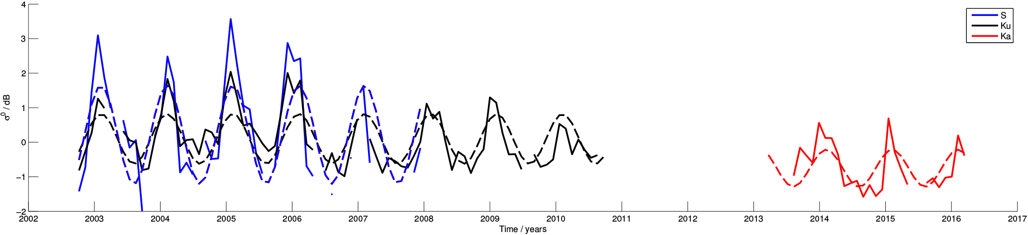
Figure 1 Time series of the backscattering coefficient at the S (blue), Ku (black) and Ka (red) bands at location (69.468^∘ S, 134.28^∘ E) between October 2002 and December 2007 at S band, October 2002 and September 2010 at Ku band and March 2013 and March 2016 at Ka band. The dashed lines represent the best fits to the time series (see Eq. 1). The observations show the seasonal cycle with a 1-year period at the different frequencies.

2.2 Amplitude and date of maximum backscattering coefficient in the seasonal cycle

The amplitude and the date at which the backscattering coefficient (σ⁰) reaches a maximum within a seasonal cycle were calculated at the S, Ku and Ka bands for the entire Antarctic continent. Figure 1 shows an example of the temporal evolution of σ⁰ at a location (69.46^∘ S, 134.28^∘ E) at the three frequencies. The time series of σ⁰ exhibit a clear and well-marked cycle with a 1-year period (called seasonal cycle hereafter). The amplitude and the phase of the seasonal cycle of σ⁰ were computed by fitting the observations with the following model Eq. (1):

$$\begin{array}{}\text{(1)}& {\mathit{\sigma }}_i^{\mathrm{0}}\left(t\right)={\mathit{\alpha }}_i\sin \left(\mathrm{2}\mathit{\pi }{\displaystyle \frac{t}{T}}\right)+{\mathit{\beta }}_i\cos \left(\mathrm{2}\mathit{\pi }{\displaystyle \frac{t}{T}}\right)+C_i,\end{array}$$

with $A_i=\sqrt{{\mathit{\alpha }}_i^{\mathrm{2}}+{\mathit{\beta }}_i^{\mathrm{2}}}$ and Φ_i = arctan (β_i∕α_i), where A_i and Φ_i is the amplitude and the phase of the seasonal cycle of ${\mathit{\sigma }}_i^{\mathrm{0}}$, respectively, deduced from constants α_i and β_i returned by the model; T = 365 days; t ranges from 0 to 5 years for the S band, from 0 to 8 years for the Ku band and from 0 to 3 years for the Ka band, with steps of 35 days; and i represents the data point over the continent. The fit was done with the ordinary least squares method and all data points with time series length less than 11 cycles (about a year) were discarded. The date at which σ⁰ reaches a maximum within a seasonal cycle is obtained by converting the seasonal phase Φ_i to fraction of a year (assuming a year counts for 360 days). We have found that along-track analysis of the seasonal parameters of σ⁰ showed no dependence to anisotropic effects. In the following, both ascending and descending measurements are mixed to keep a high density of observations and cover most AIS (∼ 1.9 million data points). For visualization needs, seasonal parameters are interpolated on a map of 5 km × 5 km grid by averaging with Gaussian weights. We considered all data points within a 25 km radius and weighted with a decorrelation radius of 10 km.

2.3 Backscattering coefficient modeling

To explore the snowpack properties that drive the seasonal cycle of σ⁰, we investigated its sensitivity to the snowpack surface and subsurface properties using an altimetric echo model of snow. This model accounts for the surface and the volume echoes. The surface echo results from the interactions of the radar wave with the snow surface (air–snow interactions) while the volume echo results from the interactions of the radar wave with the scatterers within the snowpack (snow–snow interactions). The physics involved in both surface and volume echoes have been previously studied by Lacroix et al. (2008b).

2.3.1 Surface echo modeling

The snow surface can be modeled as a randomly rough surface because most naturally occurring surfaces are irregular. The surface scattering coefficient from a rough surface is thus controlled by the effective dielectric constant of the medium and the surface roughness characteristics (Ulaby et al., 1982; Fung, 1994). The effective dielectric constant of the snow is a function of the snow density and the ice dielectric constant, while the roughness is usually modeled by two parameters: the surface correlation length (l) and the standard deviation of the surface elevation (σ_h) (Ulaby et al., 1982). In the case of large standard deviations of the surface elevation (σ_h) (compared to the radar wavelength), the backscattering coefficient from a rough surface ${\mathit{\sigma }}_{\mathrm{sur}}^{\mathrm{0}}$ can be estimated assuming a Gaussian autocorrelation function (Ulaby et al., 1982):

$$\begin{array}{}\text{(2)}& {\mathit{\sigma }}_{\mathrm{sur}}^{\mathrm{0}}={\displaystyle \frac{{\left|R\left(\mathrm{0}\right)\right|}^{\mathrm{2}}}{\mathrm{2}{S}^{\mathrm{2}}}},\end{array}$$

where R(0) is the Fresnel reflection coefficient at the normal incident angle and $S=l/{\mathit{\sigma }}_{\mathrm{h}}$ the root mean square (RMS) of the surface slope at the radar wavelength scale. Equation (2) is almost independent of the radar wave frequency and ${\mathit{\sigma }}_{\mathrm{sur}}^{\mathrm{0}}$ increases with increasing surface snow density and decreasing surface slope RMS. Surface snow density variations from 300 to 400 kg m⁻³ induce a variation of ±2.17 dB in the surface echo.

2.3.2 Volume echo modeling

The volume echo is mainly controlled by the scattering coefficient (K_s), depending on the size of the scatterers and the radar frequency. The power extinction in the snowpack is the sum of the scattering coefficient (K_s) and the absorption (K_ab) coefficient. The latter depends on snow temperature and radar frequency. In the following, the scatterers are assumed to be spherical. K_s and K_ab are given by Mätzler (1998):

$$\begin{array}{}\text{(3)}& {\displaystyle }& {\displaystyle }{K}_{\mathrm{s}}={\displaystyle \frac{\mathrm{3}}{\mathrm{32}}}{p}_{\mathrm{c}}^{\mathrm{3}}{K}_{\mathrm{0}}^{\mathrm{4}}\mathit{\nu }\left(\mathrm{1}-\mathit{\nu }\right){\left({\mathit{ϵ}}_i^{\prime }-\mathrm{1}\right)}^{\mathrm{2}}{K}_{\mathrm{d}}^{\mathrm{2}},\text{(4)}& {\displaystyle }& {\displaystyle }{K}_{\mathrm{ab}}=K_{\mathrm{0}}\mathit{\nu }{\mathit{ϵ}}_i^{\prime \prime }{K}_{\mathrm{d}}^{\mathrm{2}},\end{array}$$

where $K_{\mathrm{0}}=\mathrm{2}\mathit{\pi }/\mathit{\lambda }$ is the wave number and λ the wavelength, ν is the fractional volume of the scatterers, ${\mathit{ϵ}}_i^{\prime }$ and ${\mathit{ϵ}}_i^{\prime \prime }$ are the real and imaginary parts of the effective dielectric constant of pure ice, $p_{\mathrm{c}}=\left(\mathrm{4}{r}_{\mathrm{g}}\right)/\mathrm{3}$ (Mätzler, 1998) is the correlation length (used here as the effective size parameter) with r_g the scatterers radius and $K_{\mathrm{d}}^{\mathrm{2}}={\left|\mathrm{2}{\mathit{ϵ}}^{\prime }+\mathrm{1}\right|}^{\mathrm{2}}/{\left|\mathrm{2}{\mathit{ϵ}}^{\prime }+{\mathit{ϵ}}_i^{\prime }\right|}^{\mathrm{2}}$ with ϵ^′ the real part of the effective dielectric constant of snow (Tiuri et al., 1984).

For snow grain radius increasing from 0.3 to 0.5 mm, K_s increases from 1.05 to 4.85 m⁻¹ at the Ka band, from 0.02 to 0.08 m⁻¹ at the Ku band and from 0.58 × 10⁻⁴ to 2.7 × 10⁻⁴ m⁻¹ at the S band. As snow temperature varies from 220 to 250 K, K_ab increases from 0.194 to 0.287 m⁻¹ at the Ka band, from 0.026 to 0.039 m⁻¹ at the Ku band and from 0.002 to 0.003 m⁻¹ at the S band. The extinction coefficient at the Ka band is dominated by the scattering coefficient. In contrast, the losses by absorption dominate the extinction at the S band while at the Ku band, both coefficients are of the same order of magnitude. Volume scattering mainly affects the Ka and Ku bands. Finally, the losses by absorption increase with snow temperature while the scattering coefficient is mainly driven by snow grain size. Both the losses by absorption and scattering coefficient increase with increasing radar frequency.

Snow property profiles

For the simulations, we considered the same vertical density profile as Lacroix et al. (2008b) with a variation only in the top 10 m given by

$$\begin{array}{}\text{(5)}& \mathit{\rho }\left(z\right)={\mathit{\rho }}_{\mathrm{0}}+pz+c_{\mathrm{2}}{z}^{\mathrm{2}}+c_{\mathrm{3}}{z}^{\mathrm{3}},\end{array}$$

where c₂ and c₃ are constant values taken from the Talos Dome density profile: −1.35 × 10⁻⁴ and 5.86 × 10⁻⁷, respectively (Frezzotti et al., 2004). ρ₀ is the mean surface density and p = 1.40 × 10⁻² is calculated as a function of ρ so that the density at the depth below the surface z=10 m is the density measured at the Talos Dome (72.78^∘ S, 159.06^∘ E). The choice of the vertical density profile has a negligible effect on the results of the sensitivity test. Snow temperature is computed using the solution of the thermal diffusion equation (e.g Bingham and Drinkwater, 2000; Surdyk, 2002), assuming a sinusoidal seasonal surface temperature and constant snow thermal diffusivity κ. The temperature at depth z is of the form

$$\begin{array}{}\text{(6)}& T\left(z,t\right)=A_{\mathrm{m}}\text{exp}\left({\displaystyle \frac{-z}{l}}\right)\cos \left(\mathit{\omega }t-{\displaystyle \frac{z}{l}}\right)+T_{\mathrm{m}},\end{array}$$

where A_m and T_m are the seasonal amplitude and mean temperatures, respectively, ω is the angular frequency, t is the time, z is the depth and $l=\sqrt{\mathrm{2}\mathit{\kappa }/\mathit{\omega }}$. κ is the ratio of the thermal conductivity (κ_d) to the heat capacity and the snow density (ρ). We used the quadratic relationship of the thermal conductivity derived by Sturm et al. (1997): ${\mathit{\kappa }}_{\mathrm{d}}=\mathrm{0.138}-\mathrm{1.01}\mathit{\rho }+\mathrm{3.233}{\mathit{\rho }}^{\mathrm{2}}$. In the computing of κ_d and κ, snow density, ρ, is assumed equal to an average of the density profile of Eq. (5) (Bingham and Drinkwater, 2000). The temperature wave propagating in the snowpack has decreasing amplitude with respect to depth. The snow grain growth rate is mainly dependent on snow temperature (Brucker et al., 2010) and the snow grain profile with depth (Bingham and Drinkwater, 2000) is expressed by

$$\begin{array}{}\text{(7)}& r_{\mathrm{g}}{\left(z\right)}^{\mathrm{2}}=r_{\mathrm{0}}^{\mathrm{2}}+K_{\mathrm{g}}z/\mathit{\pi }D,\end{array}$$

where K_g=0.00042 mm² yr⁻¹ is the typical snow grain growth rate, D is the mean annual snow accumulation (mm yr⁻¹), z is the depth and r₀ is the spherical scatterer mean radius at the surface. Tests of variation of D show no significant effect on the volume echo trend, and we therefore set D to 50 mm yr⁻¹ (Bingham and Drinkwater, 2000).

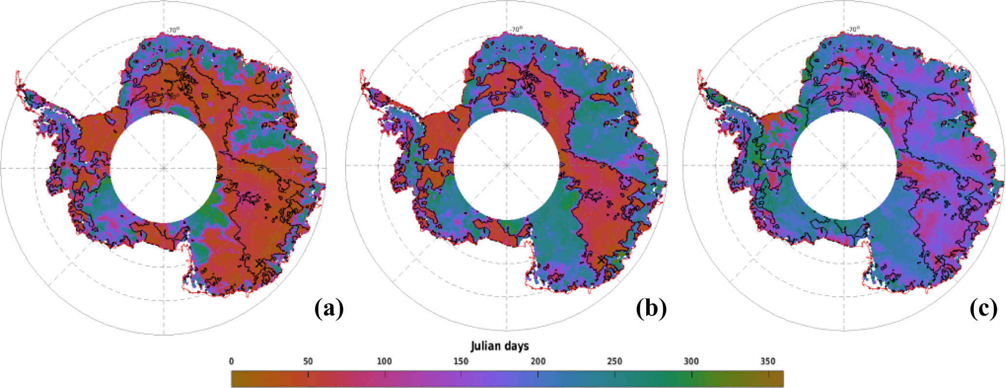
Figure 2 Spatial distribution of the seasonal date of maximum backscattering coefficient at the S (a), Ku (b) and Ka (c) bands. Black contour lines delineate regions where the backscattering coefficient at the Ku band peaks before April. Blue defines a maximum in the winter while the magenta a maximum in the summer. The cross mark represents the location of the time series shown in Fig. 1. White areas indicate regions where no observations are available (latitudinal orbit limit of 81.5^∘ S). Color bar is cyclic and defines Julian days.

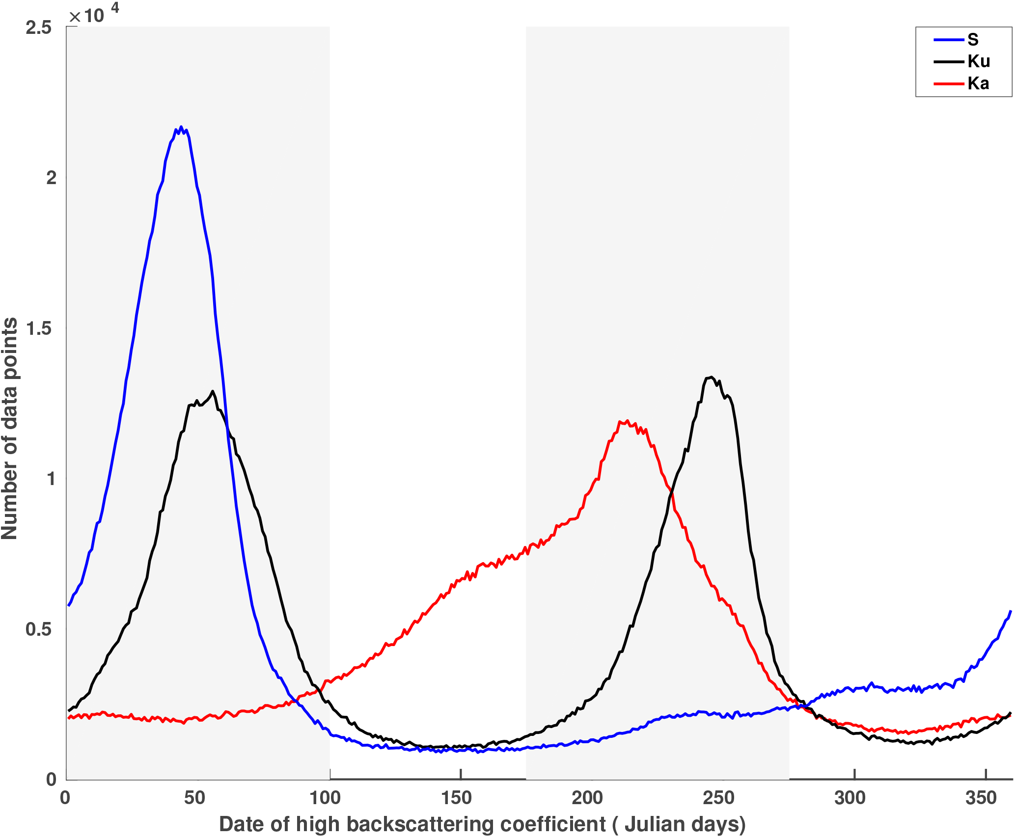
Figure 3 Histogram of the seasonal date of maximum backscattering coefficient at the S (blue), Ku (black) and Ka (red) bands. The gray bars represent periods referred to as summer (January to April) and winter (June to September).

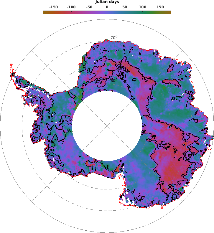
Figure 4 Difference of the seasonal date of maximum backscattering coefficient between the Ku and Ka bands. Blue defines a maximum in the Ka band before the Ku band while the magenta the inverse. Black contour lines delineate regions where the backscattering coefficient at the Ku band peaks before April. The cross mark represents the location of the time series shown in Fig. 1. White areas indicate regions where no observations are available (latitudinal orbit limit of 81.5^∘ S). The color bar is cyclic and defines the Julian days.

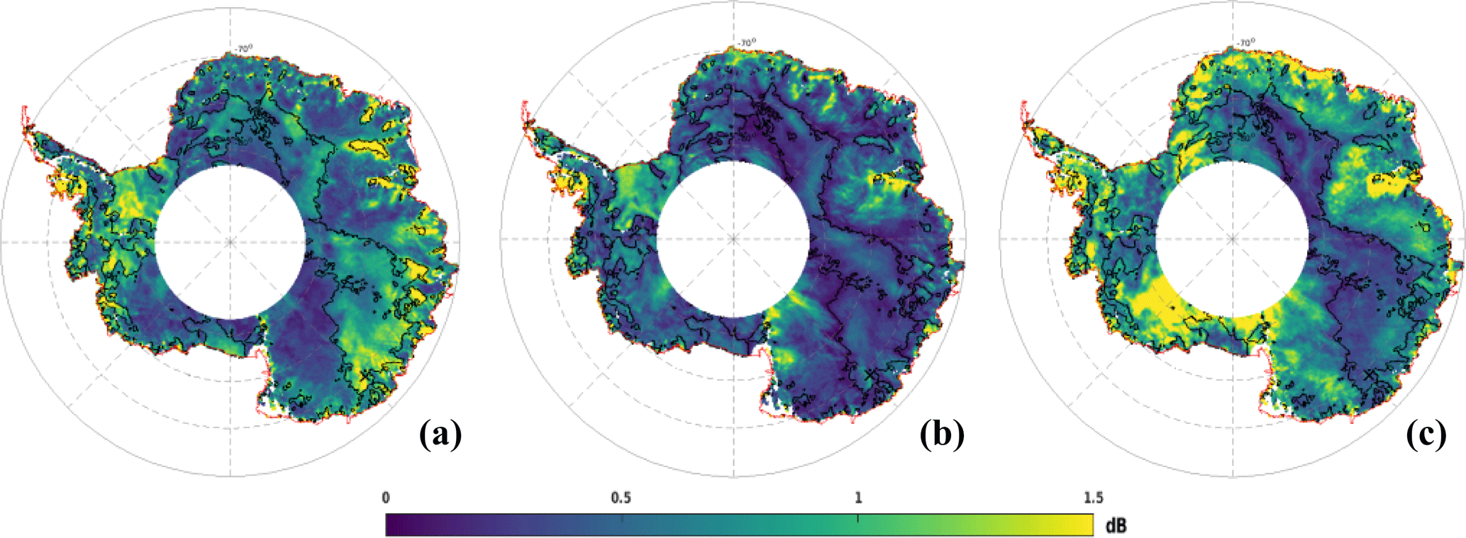
Figure 5 Spatial distribution of the seasonal amplitude of the backscattering coefficient at the S (a), Ku (b) and Ka (c) bands. Black contour lines delineate regions where the backscattering coefficient at the Ku band peaks before April. The cross mark represents the location of the time series shown in Fig. 1. White areas indicate regions where no observations are available (latitudinal orbit limit of 81.5^∘ S). Values are expressed in dB.

3 Results

3.1 Spatial patterns of the amplitude and date of maximum backscattering coefficient

The spatial distribution and the histogram of the seasonal date of maximum σ⁰ at the S, Ku and Ka bands are shown in Figs. 2 and 3, respectively. Among the three bands, the Ku band presents the most contrasted geographical patterns. In the zone that appears in magenta, the seasonal cycle of σ⁰ reaches a maximum early in the year (summer peak zone, SP hereafter). This zone covers the eastern-central part of the AIS, which encompasses the domes and high-altitude regions (∼ > 3000 m a.s.l.). It extends from Wilkes Land to Dronning Maud Land and is characterized by a decrease in σ⁰ from late fall to early spring followed by an increase at the end of the summer. The zone appearing in blue (hereafter winter peak zone, WP), encompasses the lower regions (< 3000 m a.s.l.) including coastal steeply sloped regions. It is characterized by an increase in σ⁰ from late fall to early spring. In contrast to the Ku band, the seasonal cycles of σ⁰ over the AIS are generally maximum in the summer at the S band but maximum in the winter at the Ka band. In Fig. 3, the Ku band date of maximum σ⁰ histogram is clearly bimodal with peaks between Julian days 1 and 100 (1 January to mid-April) and between Julian days 175 and 275 (June to September). In the following, these two periods are referred to as summer and winter, respectively. With these definitions, the WP and SP represent 42 and 45 % of the observed area, respectively. The histogram of the date of maximum σ⁰ at the S and Ka bands are unimodal with a peak in summer for a lower frequency (WP: 11 %, SP: 66 %, using the summer and winter periods previously defined) and a peak in winter for a higher frequency (WP: 50 %, SP: 14 %, using the summer and winter periods previously defined). The difference of the seasonal date of maximum σ⁰ between the Ku and Ka bands (Fig. 4), over the AIS, shows a geographical pattern similar to that observed in Fig. 2b. Negative values indicate that σ⁰ is maximum at the Ku band before the Ka band while positive values indicate the opposite. Negative values account for about 36 % of the observations and coincide with the SP where σ⁰ is maximum in summer at the Ku band. Positive values, the zone appearing in blue, cover 48 % of the AIS and coincide with the WP. Hence, we note a positive lag of the date of maximum σ⁰ between the Ku and Ka bands only in the zone where σ⁰ is maximum in the winter in both frequencies and a negative lag in the other zones. The spatial distribution of the seasonal amplitude of σ⁰ at the Ka band (Fig. 5c) shows an obvious geographical pattern close to that of the seasonal date of maximum σ⁰ at the Ku band. The Ka band seasonal amplitude of σ⁰ is the highest in the WP (1.02 ± 0.56 dB) and weakest in the SP (0.53 ± 0.41 dB) as shown in Fig. 6. By contrast, the seasonal amplitude of σ⁰ at the S band (Fig. 5a) appears anticorrelated with that at the Ka band, exhibiting a large seasonal amplitude in the SP (0.79 ± 0.40 dB) and a weak amplitude in the WP (0.42 ± 0.28 dB). The seasonal amplitude of σ⁰ in the SP is almost twice as large as that of the WP at the S band and the inverse is true at the Ka band. The seasonal amplitude of σ⁰ at the Ku band shows no evident regional patterns and is almost of the same magnitude in both zones (Fig. 5b), except in the interior of Wilkes Land, Princess Elisabeth Land and the Ronne Ice Shelf, which showed greater amplitudes.

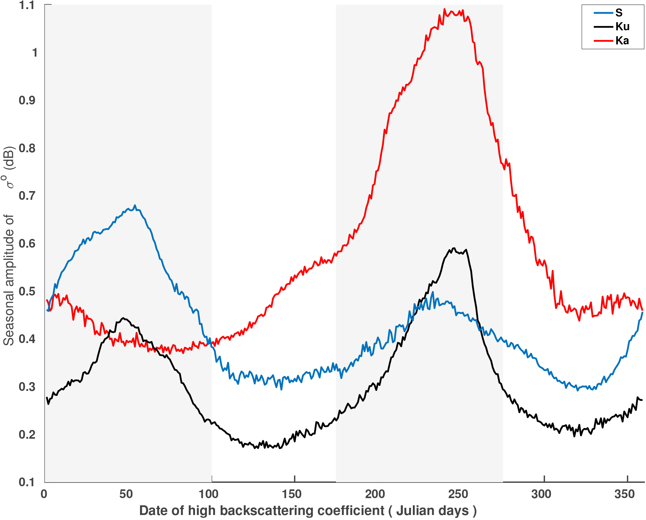
Figure 6 Mean seasonal amplitude with respect to the date of maximum backscattering coefficient at the S (blue), Ku (black) and Ka (red) bands. The gray bars represent periods referred to as summer (January to April) and winter (June to September).

3.2 Temporal variations of the surface elevation with respect to the backscattering coefficient

Figure 7 shows the spatial distribution of temporal variations of the estimated surface elevation residuals with respect to σ⁰ residuals at the Ku band, hereafter denoted dh∕ dσ⁰. The surface elevation was indirectly estimated from the retracked range (computed with the ICE-2 retracker) at each data point and was corrected for atmospheric errors. dh and dσ⁰ were derived by subtracting the mean value from the time series of the elevation and backscatter, respectively. dh∕ dσ⁰ represents the correlation gradient or the slope at each data points over the AIS. Negative values of dh∕ dσ⁰ indicate that surface elevation decreases when σ⁰ increases, implying that temporal variations in σ⁰ are due to changes in the deep snowpack properties, i.e., in the volume echo. In fact, the inverse relationship between surface elevation and σ⁰ is related to a greater backscatter from depth that shifts more power to greater delay times in the received waveform, thus increasing the retracked range and decreasing the estimated elevation (Armitage et al., 2014). In contrast, positive values of dh∕ dσ⁰ indicate that the surface elevation increases with σ⁰. In this case, the temporal variations of σ⁰ are related to changes in the surface echo. The map in Fig. 7 shows that near-zero and negative values of dh∕ dσ⁰ (in blue) are found in the WP. This means that the WP undergoes large variations of volume echo.

Figure 7 Temporal variations of the surface elevation residuals with respect to the backscattering coefficient residuals at the Ku band (denoted hereafter, dh∕ dσ⁰). Black contour lines delineate regions where the backscattering coefficient at the Ku band peaks before April. The cross mark represents the location of the time series shown in Fig. 1. White areas indicate regions where no observations are available (latitudinal orbit limit of 81.5^∘ S). Values are expressed in m dB⁻¹.

3.3 Sensitivity test

Since there are few, if any, studies on the seasonal cycle of snow surface roughness, it is poorly known. The sensitivity study of the surface echo is thus limited by the lack of information on snow surface roughness, in particular over the AIS. Consequently, we have focused on the modeling of the seasonal cycle of the volume echo. In this subsection, the sensitivity test of the volume echo at the S, Ku and Ka bands to snow properties is explored considering three parameters snow temperature, snow grain size and snow density in the analysis of the seasonal cycle of σ⁰.

The model shows an increase in the volume echo with snow density at the three frequencies (Fig. 8a). Snow density controls the thermal conductivity of the medium. Increasing surface snow density increases thermal diffusivity, which attenuates the propagation of the temperature wave in the snowpack. Figure 8b and c show that the volume echo at the S band is not sensitive to snow temperature and grain size variations, while the volume echo at the Ku and Ka bands is affected by both parameters. Snow density, temperature and grain size impacts on the volume echo are more significant at the Ka band than at the Ku and S band levels. The volume echo increases with the snow density at the three frequencies, and at the S band the volume echo is less significant.

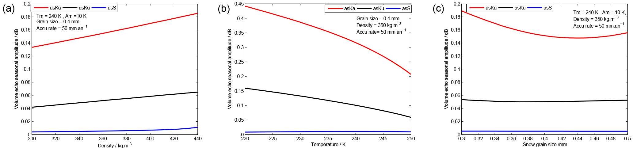
Figure 8 Sensitivity tests of the volume echo with respect to the surface snow density (a), snow temperature (b) and snow grain size (c) at the S (blue), Ku (black) and Ka (red) bands.

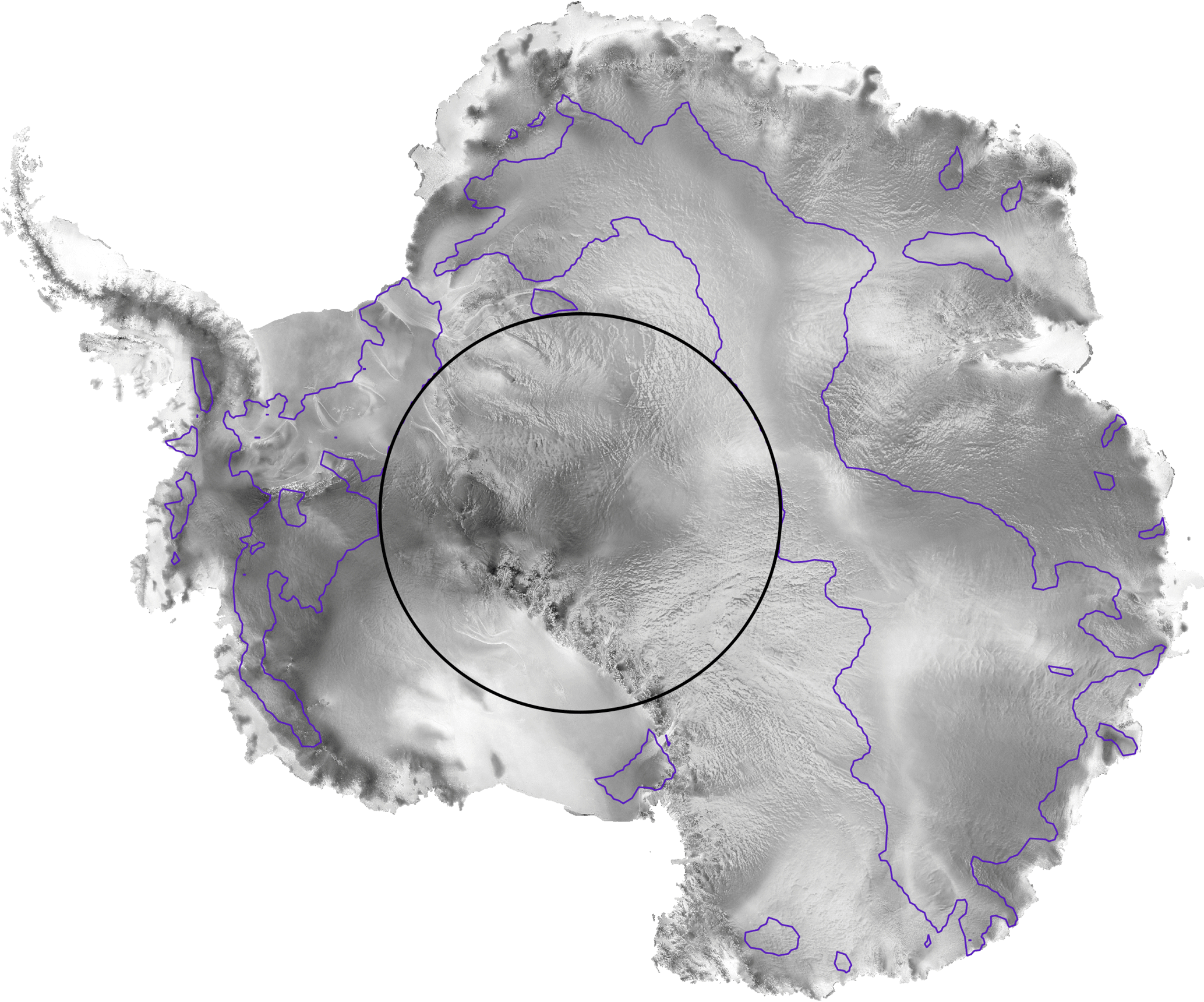
Figure 9 Distribution of the date of maximum backscattering coefficient at the Ku band superimposed on the RADARSAT mosaic (RAMP). Blue contour lines show the boundaries between the WP and the SP over the Antarctica Ice Sheet. SPs are regions where the backscattering coefficient reaches a maximum in summer (inset of the contours), and WPs are regions where the backscattering coefficient reaches a maximum in winter (where snow surface features are apparent). No observations are available beyond 81.5^∘ S (black circle).

4 Discussion

The sensitivity of the volume echo to snow temperature shown in Fig. 8b implies that the volume echo is maximum in winter at the Ku and Ka bands and constant at the S band. This sensitivity is explained by the fact that increasing snow temperature increases absorption, resulting in a decrease of the radar wave penetration in the medium and thus limiting the volume echo. Also, increasing snow grain size increases the scattering coefficient, which in turn increases the radar wave extinction in the medium. This results in a decrease of the radar wave penetration and therefore may limit the volume echo. Moreover, the positive lag observed between the Ku and Ka bands in the WP in Fig. 4 can be explained by the difference of the radar wave penetration depth between the Ku (∼ 10 m) and Ka (> 1 m) bands in the snowpack. This lag is related to the propagation of the temperature gradient from the surface into the snowpack. As the temperature controls the snow grain metamorphism and the radar wave penetration depth, the variation in the volume echo would be predominantly driven by the seasonal variations of snow temperature.

Snow density is involved in both the surface and volume echoes. The magnitude of these echoes increase with increasing surface snow density, and thus similar seasonal cycle of σ⁰ would be expected at any frequency if snow density were the main driver. This is in contrast to the observations (Fig. 3). Therefore, the seasonal cycle of σ⁰ cannot be explained solely by snow density. Being insensitive to snow temperature and grain size (Fig. 8b, c), the observed seasonal cycle of σ⁰ at the S band cannot be explained by the volume echo. This implies that snow surface properties (surface snow density and roughness) are the main factors driving the seasonal cycle of σ⁰ at the S band.

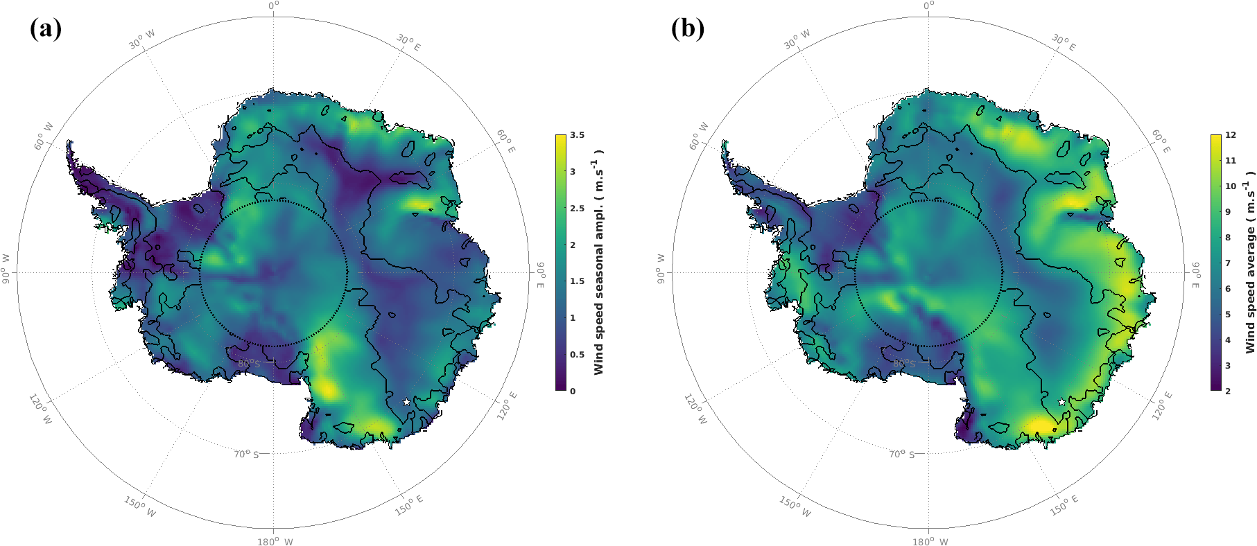
Figure 10 Seasonal wind speed amplitude (a) and average (b). Data are extracted from ERA-Interim reanalysis provided by ECMWF on 25×25 km² grid cells, from the period 2002 to 2010 corresponding to the ENVISAT lifetime. Black contour lines delineate regions where the backscattering coefficient at the Ku band peaks before April. The white star shows the location of the time series plotted in Fig. 1. No observations are available beyond 81.5^∘ S (black dotted circle).

From the S to Ka band, the radar wavelength decreases by a factor of 12 from 9.4 to 0.8 cm corresponding to a scale change from centimeter to millimeter. The scale at which the surface roughness plays a role in radar backscattering coefficient depends on the radar wavelength (Ulaby et al., 1982). On a rough surface, the surface scattering consists of two components: the coherent and incoherent scattering (Ulaby et al., 1982). The former is the scattered component in the specular direction while the latter is the scattered component in all directions. As the radar wavelength is shortened to less than a centimeter, the surface appears rougher and the surface coherent component vanishes (Ulaby et al., 1982). The surface incoherent component magnitude is small and thus is concealed by the volume scattering, which consists of only incoherent scattering. The backscattering coefficient at a smaller wavelength or on a rougher surface consists of only incoherent components and therefore appears as a volume-scattering medium. Simulations in Fig. 8 emphasize this contention, showing a greater amplitude of the volume echo at higher frequencies. We can therefore argue that the seasonal cycle of the observed σ⁰ at the Ka band is governed by the volume echo. This explains the peak of the observed σ⁰ in the winter at the Ka band over the AIS.

Several observations show that sastrugi (10 cm to 1 m height) are the main contributors to surface roughness (Kotlyakov, 1966; Inoue, 1989; Lacroix et al., 2007). Since the biggest features (hectometer to kilometer scales) change little over time, it is likely that the most influential roughness scale in the seasonal cycle of the surface echo is the sastrugi (Lacroix et al., 2008a). Despite the increase in magnitude of the surface and volume echoes with surface snow density, evidence from Fig. 3 suggests that the seasonal cycle of σ⁰ cannot be explained by the seasonal cycle in surface snow density. Therefore, it is likely that the seasonal cycle of the observed σ⁰ at the S band, predominantly driven by the surface echo, stems from the seasonal cycle of the snow surface roughness. There is no field observation that confirms this fact, but our findings suggest that such information would help to understand the altimetric signal in the future. However, in this study it is difficult to differentiate with certainty between the surface snow density and the snow surface roughness, which drives the seasonal cycle of the surface echo. There are three main reasons for this: (i) The snow surface roughness is poorly known, in particular its seasonal variability; (ii) surface snow properties evolve rapidly with the wind; and (iii) the relation between the surface snow roughness and density is complex because both variables are interdependent. The denser the snow surface, the larger the effect of surface roughness. This amplification is due to the increase of the effective dielectric discontinuity with density (Fung, 1994).

Considering that σ⁰ at the Ku band shows two opposing seasonal cycle patterns over the AIS and its wavelength is between that of the S and Ka bands, we suggest that σ⁰ at the Ku band is dominated by the seasonal cycle of the surface echo, similar to the S band in the SP, and by the seasonal cycle of the volume echo, similar to the Ka band in the WP. We support this hypothesis with ancillary data and by modeling. By overlaying the Antarctica RADARSAT mosaic with the SP boundaries (Fig. 9), we find that the WP matches regions of large heterogeneous backscatter from RADARSAT, where megadunes (Frezzotti et al., 2002) and wind-glazed surfaces (Scambos et al., 2012) have been observed. The seasonal cycle of σ⁰ at the Ku band is maximum in the winter in heterogeneous RADARSAT backscatter regions while it is maximum in the summer in the other regions. In fact, areas of megadunes are characterized by slightly steeper regional slope and the presence of highly persistent katabatic winds (Frezzotti et al., 2002) and wind-glazed surfaces have been formed by persistent katabatic winds in areas of megadunes (Scambos et al., 2012). There exists therefore a relationship between the wind and the seasonal cycle of σ⁰. To further investigate this point, we used ERA-Interim reanalysis wind speed data supplied by ECMWF (European Centre For Medium-Range Weather Forecasts) on the period 2002 to 2010, corresponding to that of the Ku band. Equation (1) is used to compute the seasonal characteristics of the wind speed by replacing σ⁰ with the wind speed. A visual inspection shows a high spatial coherence of the seasonal amplitude of the wind speed (Fig. 10a) patterns with the date of maximum σ⁰ over the seasonal cycle at the Ku band (Fig. 2b). Wind speed average (8.2 ± 1.6 m s⁻¹) and seasonal amplitude (1.7 ± 0.4 m s⁻¹) are higher in the WP than in the SP (6.6 ± 1.58 m s⁻¹ and 1.0 ± 0.3 m s⁻¹, respectively).

The striking similarity in the spatial distribution of the seasonal amplitude of σ⁰ at the Ka band (Fig. 5c) and the seasonal date of maximum σ⁰ at the Ku band (Fig. 2b), which is itself correlated to the seasonal amplitude of the wind speed (Fig. 10a), suggests that the wind plays a significant role in the spatial distribution of the seasonal amplitude of σ⁰ at the Ka band. Although the wind effects on the snowpack are numerous and complex, we retained two for which we simulated the impacts on the volume echo (Fig. 8):

• a.

  Wind may smash snow grains so that the surface snow density increases with wind speed (Male, 1980); this leads to an enhancement of the volume echo at the three frequencies as shown in Fig. 8a. Surface snow density is a good candidate for explaining the spatial distribution of the seasonal amplitude of σ⁰ at the Ka band because snow compaction can occur at different times of the year depending on the snow accumulation rate and the temperature gradient (Li and Zwally, 2002, 2004).

• b.

  Increasing wind speed leads to an increase in snow erosion and transport that removes all or almost all the precipitated or wind deposited snow that may temporarily accumulate (Scambos et al., 2012; Lenaerts et al., 2012). This implies that there is no significant change in the surface mass balance over an annual cycle, i.e., near-zero net accumulation (Scambos et al., 2012), allowing snow surface to be almost constant and smooth. This corroborates our contention that the seasonal variation of the observed σ⁰ at the Ku band in the WP emanates exclusively from the volume echo (i.e., a greater backscatter from depth). Thus, it is presumed that these variations are due to depth hoar formation during winter in the WP. Indeed, the wind speed is on average maximum between Julian days 170 and 230 (June to August), when air temperature is colder than the snow temperature. Cold and persistent winds may unusually accelerate the cooling of the surface snow temperature (Remy and Minster, 1991). This causes an important temperature gradient, which determines the rate of metamorphism of snow grains within the snowpack. This specific increase of the temperature gradient would promote the formation of depth hoar in winter (Champollion et al., 2013), which creates coarse cup-shaped ice crystals, acts as more effective volume scatterers and hence increases the volume echo magnitude as predicted in Fig. 8c. For instance, Brucker et al. (2010) have found the highest vertical gradient in grain size, obtained over a multiyear average from 1987 to 2002, in the regions of the WP.

Finally, the combined effects of wind speed and temperature may explain the observed difference between the seasonal cycle of σ⁰ at the Ka and Ku bands. Similarly, the spatial distribution of the seasonal amplitude of σ⁰ at the Ka band is ascribed to the wind effects mentioned above on the snowpack.

5 Conclusions

This study, using 35-day repeat radar altimetry data, carries out spatial and temporal comparative analysis of the seasonal amplitude and date of maximum σ⁰ at the S, Ku and Ka bands. We used an 8-year time series of σ⁰ for the Ku band, a 5-year time series of σ⁰ for the S band and a 3-year time series of σ⁰ for the Ka band, covering the time period of 2002 to 2010 for ENVISAT sensors and 2013 to 2016 for the SARAL/AltiKa sensor. The backscattering coefficient shows seasonal variations with varying amplitude and phase over the AIS and with a marked dependence on radar frequency. In general, it is maximum in winter at the Ka band and maximum in summer at the S band. At the Ku band, both behaviors are found with a maximum in the winter in the so-called WP and a maximum in the summer in the SP.

We investigated snow properties that dominate the seasonal changes in the volume echo with electromagnetic models of the backscattering coefficient. As a result, we showed that variations in snow properties, such as temperature and grain size, cannot explain the seasonal cycle of σ⁰ observed at the S band due to its small sensitivity to those parameters. In contrast, the temperature cycle reasonably explain the seasonal cycle of the observed σ⁰ at the Ka band. We explain that the contrasted seasonal cycle of the observed σ⁰ at the Ku band is due to its high sensitivity to the volume echo in the WP and to the surface echo in the SP. The geographical patterns of the WP and SP are related to the seasonal amplitude of the wind speed. This is a result of the presence or lack of wind-glazed surfaces, induced by strong and persistent winds in the megadune areas.

This investigation provides new information on the Antarctic Ice Sheet surface seasonal dynamics and provides new clues to build a robust correction of the altimetric surface elevation signal. Multi-frequency sensors are the key for improving the understanding of the physics of radar altimeter measurements over the AIS. An important limitation of this study is the lack of information on the seasonal variability of the snow surface roughness in Antarctica, which will be the topic of future work.