the Creative Commons Attribution 4.0 License.
the Creative Commons Attribution 4.0 License.
 | 04 May 2018
On the need for a time- and location-dependent estimation of the NDSI threshold value for reducing existing uncertainties in snow cover maps at different scales
Stefan Härer
Matthias Bernhardt
Matthias Siebers
Karsten Schulz
Knowledge of current snow cover extent is essential for characterizing energy and moisture fluxes at the Earth's surface. The snow-covered area (SCA) is often estimated by using optical satellite information in combination with the normalized-difference snow index (NDSI). The NDSI thereby uses a threshold for the definition if a satellite pixel is assumed to be snow covered or snow free. The spatiotemporal representativeness of the standard threshold of 0.4 is however questionable at the local scale. Here, we use local snow cover maps derived from ground-based photography to continuously calibrate the NDSI threshold values (NDSIthr) of Landsat satellite images at two European mountain sites of the period from 2010 to 2015. The Research Catchment Zugspitzplatt (RCZ, Germany) and Vernagtferner area (VF, Austria) are both located within a single Landsat scene. Nevertheless, the long-term analysis of the NDSIthr demonstrated that the NDSIthr at these sites are not correlated (r = 0.17) and different than the standard threshold of 0.4. For further comparison, a dynamic and locally optimized NDSI threshold was used as well as another locally optimized literature threshold value (0.7). It was shown that large uncertainties in the prediction of the SCA of up to 24.1 % exist in satellite snow cover maps in cases where the standard threshold of 0.4 is used, but a newly developed calibrated quadratic polynomial model which accounts for seasonal threshold dynamics can reduce this error. The model minimizes the SCA uncertainties at the calibration site VF by 50 % in the evaluation period and was also able to improve the results at RCZ in a significant way. Additionally, a scaling experiment shows that the positive effect of a locally adapted threshold diminishes using a pixel size of 500 m or larger, underlining the general applicability of the standard threshold at larger scales.
- Article
(3261 KB) - Full-text XML
- BibTeX
- EndNote


Numerous studies ranging from the local to the global scale have underlined the influence of snow cover on, e.g. air temperature, runoff generation, soil temperature and soil moisture (Bernhardt et al., 2012; Deb et al., 2015; Dutra et al., 2012; Dyurgerov, 2003; Liston, 2004; Mankin and Diffenbaugh, 2015; Santini and di Paola, 2015; Tennant et al., 2015). Hence, accurate estimation of the spatial extent of the snow pack is fundamental for a suite of applications (Pomeroy et al., 2015). The accuracy of weather and climate models heavily depends on this information, as the range of surface temperatures is instantly limited to a maximum of 0 ∘C in presence of snow and the surface albedo typically becomes significantly enhanced (Agosta et al., 2015; Liston, 2004; Rangwala et al., 2010; Takata et al., 2003; Vavrus et al., 2011). From a hydrological point of view, the formation of snow pack has a buffering effect and thus often transfers precipitation water from the cold to the warm season of the year (Bernhardt et al., 2014; Viviroli et al., 2011). This leads to an increase in summer runoff which can be beneficial to agriculture or sanitary water supply, but which can also lead to an intensification of flood events, for example in the case of rain-on-snow events (Viviroli et al., 2011). With this in mind, information on the current snow distribution is elementary for water resources management (Thirel et al., 2013) and weather forecasting model systems (Dee et al., 2011).
Snow cover distribution is often derived from satellite data and then either used as input for operational models (Butt and Bilal, 2011; Dee et al., 2011; Homan et al., 2011; Tekeli et al., 2005) or for the offline evaluation of modelled snow cover (Bernhardt and Schulz, 2010; Warscher et al., 2013) and snow fall patterns (Maussion et al., 2011). The used snow-cover mapping approaches can be grouped into four categories: manual interpretation, spectral mixture analysis and classification-based and index-based methods. Manual interpretation and classification-based approaches are often used in local snow cover mapping studies. Both are out of the scope of this study as the need for expert knowledge and high time demands limit their applicability for large time series data. Spectral mixture analysis is also not in the focus of this study as it needs an extensive spectral database for the different land surface components (Sirguey et al., 2009; Painter et al., 2009). These databases are usually not commonly available and only the final snow cover product can be downloaded (TMSCAG for Landsat and MODSCAG for MODIS). We focus on the automatic normalized-difference snow index (NDSI) approach here. It was developed by Dozier (1989) and is a simple and established method to identify snow cover in optical satellite images. NOAA/NESDIS, which is assimilated into ERA/Interim (Dee et al., 2011; Drusch et al., 2004), and the widely used MODIS snow cover products (Hall and Riggs, 2007; Hall et al., 2002) make use of the NDSI.
The NDSI can be traced back to band rationing techniques (Kyle et al., 1978; Dozier, 1984) related to the NDVI (Rouse Jr. et al., 1974; Tucker, 1979) and is based on the physical principle that snow reflection is significantly higher in the visible range of the spectrum than in mid-infrared. The index ranges between −1 and 1 and a differentiation between snow and no snow is based on an NDSI threshold value (NDSIthr) which is commonly assumed to be 0.4 (Dozier, 1989; Hall and Riggs, 2007; Sankey et al., 2015). According to Hall et al. (2001) the accuracy for monthly snow detection using the atmospherically corrected MODIS product (MOD10/MYD10) with its standard threshold is respectively about 95 % and about 85 % in non-forested and forested areas. These accuracies make NDSI-based snow cover products well suited for global-scale applications, but uncertainties have to be expected at the local scale (Härer et al., 2016). Moreover, the snow detection algorithm for the MODIS snow cover product changed in the latest Collection 6. The algorithm now uses an NDSI threshold of zero together with a flag system to detect snow cover, and users are encouraged to use their own NDSI threshold in the MODIS Snow Products Collection 6 User Guide if a binary snow cover map is desired.
In line with this, numerous recent studies have questioned the general applicability of a standard NDSIthr in local snow and glacier monitoring. When calibrating the NDSIthr manually or with automated methods against field data for single scenes, large deviations from the standard value of 0.4 have been observed. The published values range from 0.18 to 0.7 (Burns and Nolin, 2014; Härer et al., 2016; Maher et al., 2012; Racoviteanu et al., 2009; Silverio and Jaquet, 2009; Yin et al., 2013). The wide range of values show the spatiotemporal variability of the NDSIthr and raise the demand for a valid non-subjective method to define this value.
Maher et al. (2012), for example, assumed a spatially calibrated NDSIthr of 0.7 to be constant over time. The comprehensive work of Yin et al. (2013) compared various automatic entropy-based, clustering-based and spatial threshold methods to adjust the NDSIthr for specific satellite images. The findings of Yin et al. (2013) are based on single-date comparisons at five sites around the world and were undertaken on a regional scale. The clustering-based image segmentation method developed by Otsu (1979) compared best to the evaluation data sets, which is why the Otsu method is used as comparative data here.
Härer et al. (2016) presented a calibration strategy for satellite-derived snow cover maps on the basis of local camera systems. The results achieved show that NDSIthr can be distinctly different during the snow cover period and that there is a need for temporal adaption of NDSIthr to achieve valid results in view of the local snow-covered area (SCA).
The aim of this study is to evaluate the variability of NDSIthr in space and time and to test if this variability leads to significant uncertainties in the existing snow cover maps. A scaling exercise which has investigated up to which scale a locally adapted threshold can improve the classification results shows the limits of the fixed threshold approach at the local scale.
We use the camera-based calibration approach (Härer et al., 2013) as reference as it has shown low error margins in comparison to high-resolution locally derived 1 m resolution snow maps at RCZ (Härer et al. 2016). The results achieved by this approach are then compared to the automatic segmentation method of Otsu (1979), which is proven to be one of the best-performing snow detection methods available today (Yin et al., 2013), to the standard threshold of 0.4 and to a location-specific threshold of 0.7 (Maher et al., 2012). Moreover, we present a seasonal model calibrated with the NDSI threshold time series. The quadratic polynomial model can also be locally adapted by including a geology-dependent offset which is comparable to earlier findings of Chaponnière et al. (2005). The results will reveal the performance of the different approaches and will clarify for which scales a fixed NDSI threshold can be an adequate solution.

Figure 1The figure shows the two test sites used in this study and their location within a Landsat scene, with the camera location in yellow, the catchment area outlined in black and the digital elevation model (DEM) superimposed on a LandsatLook image. (a) Research Catchment Zugspitzplatt (Germany), (b) Vernagtferner catchment (Austria), (c) Landsat scene (LandsatLook image, WRS2 path 193, row 27) which contains both sites.
This study focuses on two mountain sites in the European Alps, the Research Catchment Zugspitzplatt (RCZ) located in Germany (47∘40′ N, 11∘00′ E; Bernhardt et al., 2015; Weber et al., 2016) and the Vernagtferner (VF) catchment in Austria (46∘52′ N, 10∘49′ E; Fig. 1a–c; Abermann et al., 2011). RCZ is a partly glacierized headwater catchment with a spatial extent of about 13.1 km2. It stretches from 1371 to 2962 m a.s.l. The substrate is mainly limestone. VF is also an alpine headwater basin with a size of 11.5 km2 and a glaciated part of about 7.9 km2 (Mayr et al., 2013). It ranges from 2642 to 3619 m a.s.l. and the underlying rock is gneiss.
The sites are equipped with similar single-lens reflex camera systems for monitoring wide parts of the catchments starting from May 2011 at RCZ and from August 2010 at VF. The photographs are recorded as 8-bit data with three colour channels (red, green and blue; RGB) on an hourly basis for RCZ and 3 times a day for VF. The camera locations at the study sites are depicted in Fig. 1a and b and the camera orientations are south-west at RCZ and west–north-west at VF. Both investigation areas are located within a single Landsat scene (Fig. 1c), which guarantees comparable illumination conditions and allows for a direct comparison of the NDSIthr between the sites.
Overall, 156 Landsat scenes from Landsat 5 TM, 7 ETM+ and 8 OLI were available for the observation period between 18 August 2010 and 31 December 2015. Suitable satellite image–photograph pairs were available for 15 dates for RCZ and VF, for 1 date for RCZ and for 32 dates for VF only. The differences stem from the local weather conditions, from the different lengths of the local photograph time series and from the restriction that an NDSIthr calibration with PRACTISE or the clustering-based image segmentation from Otsu (1979) can only be applied if the area is not fully snow covered. For the photo rectification part of our study, we use digital elevation models (DEM), with a horizontal resolution of 1 m of RCZ and VF, and orthophotos, with sub-metre spatial resolution and topographic maps as additional material to ensure optimal geometric accuracy.
Our study investigates the differences of automatically derived NDSIthr from (a) Landsat satellite imagery and (b) terrestrial photography with literature values and displays their effects on the resulting snow cover maps. Radiometrically and geometrically corrected Landsat Level 1 data were used in combination with the cloud and shadow masking software Fmask of Zhu et al. (2015). Any pixel with a cloud probability exceeding 95 % in this analysis was excluded with a surrounding buffer of three pixels (Härer et al., 2016). The top-of-atmosphere reflectance values were calculated according to the Landsat user handbook but no atmospheric correction was applied to the Landsat data to facilitate a direct comparison to many studies that apply the NDSI for snow cover mapping, especially in high-elevation areas where atmospheric influence is known to be low (Bernhardt and Schulz, 2010; Maher et al., 2012; Warscher et al., 2013).
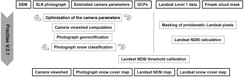
Figure 2Input and output data and the workflow of PRACTISE (version 2.1) used to generate the calibrated NDSI snow cover maps from Landsat data (from Härer et al., 2016).
The normalized-difference snow index (NDSI) was calculated according to Dozier (1989) by using green (∼ 0.55 µm) and mid-infrared (MIR, ∼ 1.6 µm) reflectance values:
NDSI values can range between −1 and 1 and the NDSIthr defines the NDSI value from which the satellite pixel is assumed to be snow covered. We used fixed values and dynamically derived NDSIthr values during this study. In the case of the fixed values, the standard of 0.4 and another literature value of 0.7 (Maher et al., 2012) were used. For the dynamic approaches, the clustering-based image segmentation approach from Otsu (1979) and a terrestrial camera-based calibration approach of Härer et al. (2016) were applied.
By using Otsu (1979), the NDSIthr was calibrated by maximizing the between-class variance of the two classes snow and no snow:
where Ps and Pns are the probabilities of the classes snow and no snow with respect to the NDSIthr, and μs and μns are the mean values of these two classes. The probability of Ps is thereby calculated as the number of pixels with NDSI values above the NDSIthr divided through the total number of pixels in the image. Pns calculates the absolute difference of Ps to 1.
We further restricted the satellite image area used for deriving NDSIthr according to Otsu (1979) to the catchment area of RCZ and VF to allow for a spatiotemporally variable NDSI threshold value within the satellite scenes investigated. Moreover, this definition facilitated direct comparison between the locally derived thresholds using the Otsu method and our own method presented in the next paragraph.
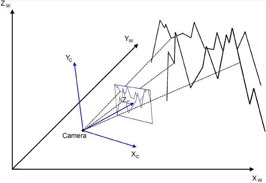
Figure 3Schematic relationship between the camera location and orientation, and the two-dimensional photograph (blue) and three-dimensional real world coordinate system (black). The dashed line connects the locations of three exemplary ground control points of the photograph with the real world for clarification.
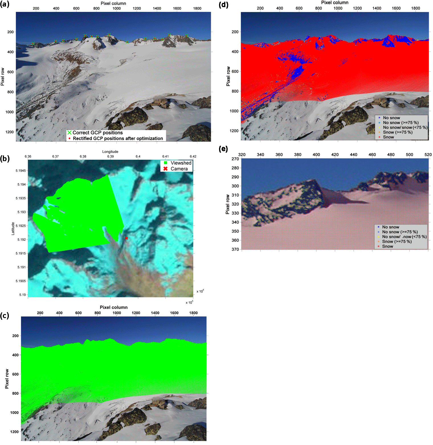
Figure 4Internal processing steps within a single PRACTISE evaluation are shown for a photograph of VF on 17 November 2011. The figures chronologically show the routines for the photograph processing in PRACTISE which are (a) the optimization of the camera location and orientation using ground control points, (b) the viewshed analysis performed using the resulting camera location and orientation, (c) the projection and (d) the classification of visible DEM pixels. More details of the PCA-based classification results in (d) can be seen in an enlarged view in (e).
The second dynamic method to calibrate the NDSIthr of the Landsat data for RCZ and VF used ground-based photographs as baseline. The Matlab software PRACTISE (version 2.1; Härer et al., 2013, 2016) was utilized first to georectify the available terrestrial photographs and secondly to calibrate the NDSIthr. To do so, overlapping areas in the photograph–satellite image pairs were used. For further understanding, Fig. 2 gives a general overview of the needed input, the internal processing steps and the generated output data of PRACTISE 2.1. The first program part georectified the photographs and computed differences between areas with and without snow. This results in a high-resolution photography-based snow cover map (Fig. 2, left column). The second part calibrated the NDSIthr for the satellite scene of interest and used the achieved value to calculate an NDSI-based satellite snow cover map (Fig. 2, right column).
The photo georectification is based on the assumption that the recorded two-dimensional photograph (Fig. 3, blue colour) is geometrically connected to the three-dimensional real world (Fig. 3, black colour). Georectification is possible if the camera type, lens and sensor system, location and orientation are known and if a high-resolution digital elevation model (DEM) is available.
Having this theoretical background in mind, we outlined the different processing steps for a photograph and a Landsat 7 scene of VF on 17 November 2011 (Figs. 4a–e and 5a–c). Before the PRACTISE program was used, any possible distortion effects of the photograph caused by the camera lens were removed by utilizing the freely available Darktable software (http://www.darktable.org/, last access: 2 May 2018) and LensFun parameters (http://lensfun.sourceforge.net/, last access: 2 May 2018). Once all data were available and ready, the PRACTISE program evaluation could start.
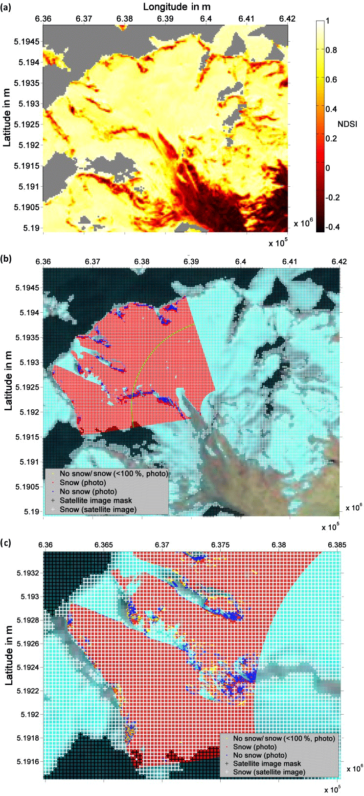
Figure 5We outline here the internal processing steps within the remote sensing routines of PRACTISE. The Landsat NDSI map from 17 November 2011 is shown in (a). Clouds and shadows (grey areas) are excluded using Fmask. The photograph and satellite snow cover map derived from the PRACTISE evaluation are superimposed on the LandsatLook image of 17 November 2011 in (b). Snow is depicted in red in the photograph snow map and white in the satellite snow map. The lower areas at VF (south-east of the green line in (b) were excluded from the complete analysis. The close-up in (c) clarifies which photographed areas are part of the analysis and additionally underlines the high agreement between photograph and satellite snow cover map. The maps are projected in the Universal Transverse Mercator (UTM) system based on the World Geodetic System 1984 (WGS84).
In the first step, information about the camera location and orientation was needed for georectification of the photography. This information was automatically optimized by using ground control points (GCPs, Fig. 4a; Sect. 3.3 in Härer et al., 2013). The calculated viewpoint and viewing direction were by default used to perform a viewshed analysis (Fig. 4b; Sect. 3.1 in Härer et al., 2013). The viewshed was needed for identification of areas which were visible from the viewpoint and which were not obscured by topographical features or within a user-specified buffer area around the camera. The respective DEM pixels were then projected to the photo plane (Fig. 4c; Sect. 3.2 in Härer et al., 2013).
Then, the snow classification module was activated to differentiate between snow-covered and snow-free DEM pixels (Fig. 4d). Two major procedures were available for classification: statistical analysis which used the blue RGB band (Salvatori et al., 2011; Sect. 3.4 in Härer et al., 2013) and an approach based on principal component analysis (PCA; Sect. 3.1 in Härer et al., 2016). The first was used for shadow-free scenes, the second for scenes with shaded areas. Section 3.4 in Härer et al. (2013) gives more insights into a third manual option if none of the two classification routines could be applied successfully. Moreover, it was shown in Sect. 4 in Härer et al. (2013) that even if a wrong classification algorithm was applied, no more than 5 % of the pixels in the error-prone parts of the photograph snow cover map were misclassified. It was also shown in an earlier publication that the classification of shadow-affected photographs are of the same quality as photographs without shadows (Sect. 4 in Härer et al., 2016). As for this study, every classified image was visually inspected and no major snow classification errors comparable to our worst case example in the previous publication were found; we expect a relative misclassification error of 1 %. For the example photograph of VF on 17 November 2011, the snow classification algorithm utilizing PCA was selected to account for the shadow-affected areas in the upper left part of the photograph (Fig. 4d, enlarged view in Fig. 4e).
After the photograph rectification and classification, the remote sensing routine of PRACTISE began with the identification of satellite pixels that spatially overlap with the photograph snow cover map (Sect. 3.2 in Härer et al., 2016). The photograph and satellite image used were thereby recorded within 1 (RCZ) to 3 h (VF). Moreover, a cloud- and shadow-free satellite image is generated by using Fmask (Zhu et al., 2015). The NDSI map required was calculated according to Eq. (1) of PRACTISE (Fig. 5a).
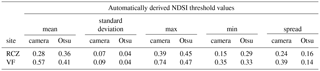
Table 1Basic statistics of the automatically derived NDSI threshold time series at RCZ and VF using the Otsu segmentation method and the camera-based calibration method.
If both the NDSI satellite map and the corresponding high-resolution photograph snow cover map were processed, the iterative calibration of the NDSI threshold value was begun. The Landsat image was thereby resampled to the finer resolution of the photograph snow cover map in the calibration to avoid losing any information through aggregation. The best agreement between the local-scale (photograph) and the large-scale (Landsat) snow cover maps was detected by maximizing accuracy, which is the ratio of identically classified pixels to the overall number of photograph–satellite image pixel pairs n (Aronica et al., 2002):
a represents the number of correctly identified snow pixels and d the same for no snow pixels. F is between 0 and 1 and becomes 1 for perfect agreement between the two images. The calibrated NDSI threshold was finally applied to the original Landsat data with 30m pixel size to generate the final Landsat snow cover map. Figure 5b shows the resulting satellite snow cover map superimposed on the photograph snow cover map and a LandsatLook image. A close-up is shown for more detail in Fig. 5c.
The glacier retreat between DEM production years (2007, 2010) and over the analysis period 2010–2015 resulted in a discrepancy between real world elevations and the available DEMs, especially in the last years of the observation period. Figure 6 exemplarily depicts the glacier retreat between 2007 and 2010 by superimposing the ice mass loss on an orthophoto of VF from 2010. This loss in elevation leads to inaccuracies in the georectification results of the photographs. Additionally, testing the 28 August 2010 photograph by applying the DEM of 2007 and 2010 showed that these georectification issues in turn affect the NDSIthr calibration results. For the DEM from 2007, the calibrated NDSIthr is 0.47, while the correct threshold for the up-to-date DEM from 2010 is 0.52. As a consequence, we limited the analysis to higher elevated and thus colder areas of the catchment where glacier retreat is marginal (areas north-west of the green line in Figs. 5b and 6).
To ensure that reducing the spatial overlap between photograph snow cover map and NDSI satellite map does not have any negative effect on the calibrated NDSIthr, we firstly calibrated the NDSIthr for the three investigated Landsat scenes in 2010 for the complete and the upper area only. Moreover, we calibrated the NDSIthr for the 44 remaining scenes between 2011 and 2015 using the upper area DEM from 2007 and 2010 to test for NDSIthr sensitivity in the longer time series. For both approaches, the differences between the calibrated NDSIthr never become larger than 0.01. Hence, we assume that our calibration approach of using the higher elevated areas at VF which is incorporated in PRACTISE by excluding a radius of 1800 m around the camera from the analysis (green line in Figs. 5b and 6) is valid for the complete analysed time series between 2010 and 2015. As we did not find a similar effect on the NDSIthr calibration in our tests at RCZ, there was no need to remove the glacier areas at RCZ from the analysis.
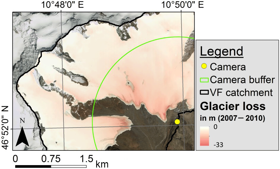
Figure 6Glacier retreat from 2007 to 2010 causes a loss in elevation of up to −33 m at VF. The green line depicts the buffer distance around the camera which was excluded from the analysis due to significant glacier loss which in turn led to geometric inaccuracies in the photograph rectification and incorrect NDSI threshold calibration results.
The NDSI thresholds derived by the two dynamic methods are now discussed and related to static thresholds. The NDSIthr predicted by the Otsu method are densely grouped around 0.4. This is underlined by a mean of 0.36 and a standard deviation of 0.04 at RCZ and a mean of 0.41 with a corresponding standard derivation of 0.04 at VF (Table 1). The statistics do not include two dates at VF as no separating NDSIthr could be found by using the Otsu method here (squares in Fig. 7a). This contradicts the real situation as the photographs show that there was no full snow coverage at the respective dates which would generally allow for prediction of NDSIthr. This shows that the application of the Otsu method is potentially uncertain in nearly fully snow-covered situations. Furthermore, the small and thus almost negligible differences with the standard of 0.4 do not justify the additional effort of using a location-dependent threshold prediction like the Otsu method. Additionally, the weak seasonal dynamics which can be found at VF also do not require time-dependent calculation of the threshold.

Figure 7The figure displays in (a) the complete time series of adjusted NDSI thresholds using the Otsu segmentation method (circles, erroneous thresholds as squares) at RCZ (red) and VF (blue) and depicts in (b) the camera-calibrated NDSI thresholds at these two sites utilizing ground-based photographs as in situ measurements (blue pluses for VF and red crosses for RCZ). Relative SCA changes at RCZ and VF resulting from the application of the standard instead of the camera-calibrated reference NDSI threshold are shown in (c).
The camera-based method leads in general to a more dynamic NDSIthr in time and to a higher systematic difference of NDSIthr between the two sites. The archived 16 NDSIthr at RCZ and 47 NDSIthr at VF are compared in a first step. The presumption of a comparable NDSIthr for both sites could not be confirmed in this case. Significant differences were detected despite the fact that both sites are high alpine and are located within a single Landsat scene. Moreover, the calibrated NDSIthr were in large parts significantly different than the standard value of 0.4. Figure 7b and Table 1 illustrate the variability and the range of NDSIthr at both sites. The minimum value at RCZ is 0.15 while the maximum value is 0.39. The values at VF are generally higher and range between 0.35 and 0.74. Values at both sites thus strongly scatter around their catchment-specific mean value (0.28 at RCZ, 0.57 at VF) but show characteristic development over the year (Fig. 8), which is also detected in a weaker form for the Otsu method at VF. Independent of the fact that this seasonal dynamic is comparable for both sites using the camera-based method, Fig. 7b highlights that the correlation coefficient between NDSIthr at RCZ and VF is very low when they are compared on a date-by-date basis (r = 0.17). By contrast, a correlation between the Otsu method and the terrestrial camera-based method at VF of −0.56 is found, which however cannot be observed at RCZ between the two methods (r = 0.10, Fig. 7a and b).
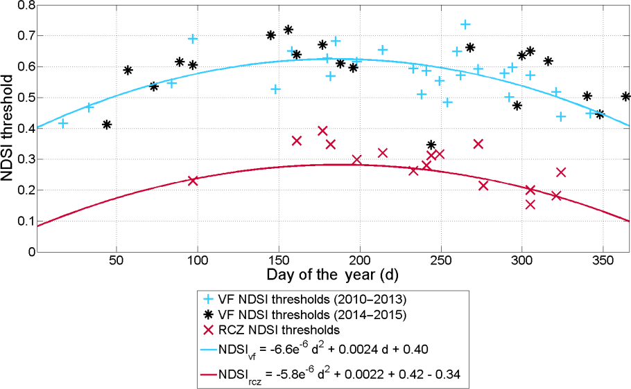
Figure 8Estimates of NDSI threshold values at VF are predicted by a quadratic polynomial model (NDSIvf, blue line) which was fitted for each day of the year to the calibrated NDSI thresholds between 2010 and 2013 (NDSIthr, blue pluses). The black asterisks represent the NDSIthr from 2014 to 2015 at VF used for evaluation of NDSIvf. Additionally, an NDSIthr prediction model for RCZ (NDSIrcz, red line) is defined by a quadratic polynomial model fitted to the complete time series of calibrated NDSIthr at VF (blue pluses and black asterisks, r2 = 0.36, RMSE = 0.07) and an additional term of −0.34. NDSIrcz is evaluated against the calibrated NDSIthr of RCZ (red crosses).
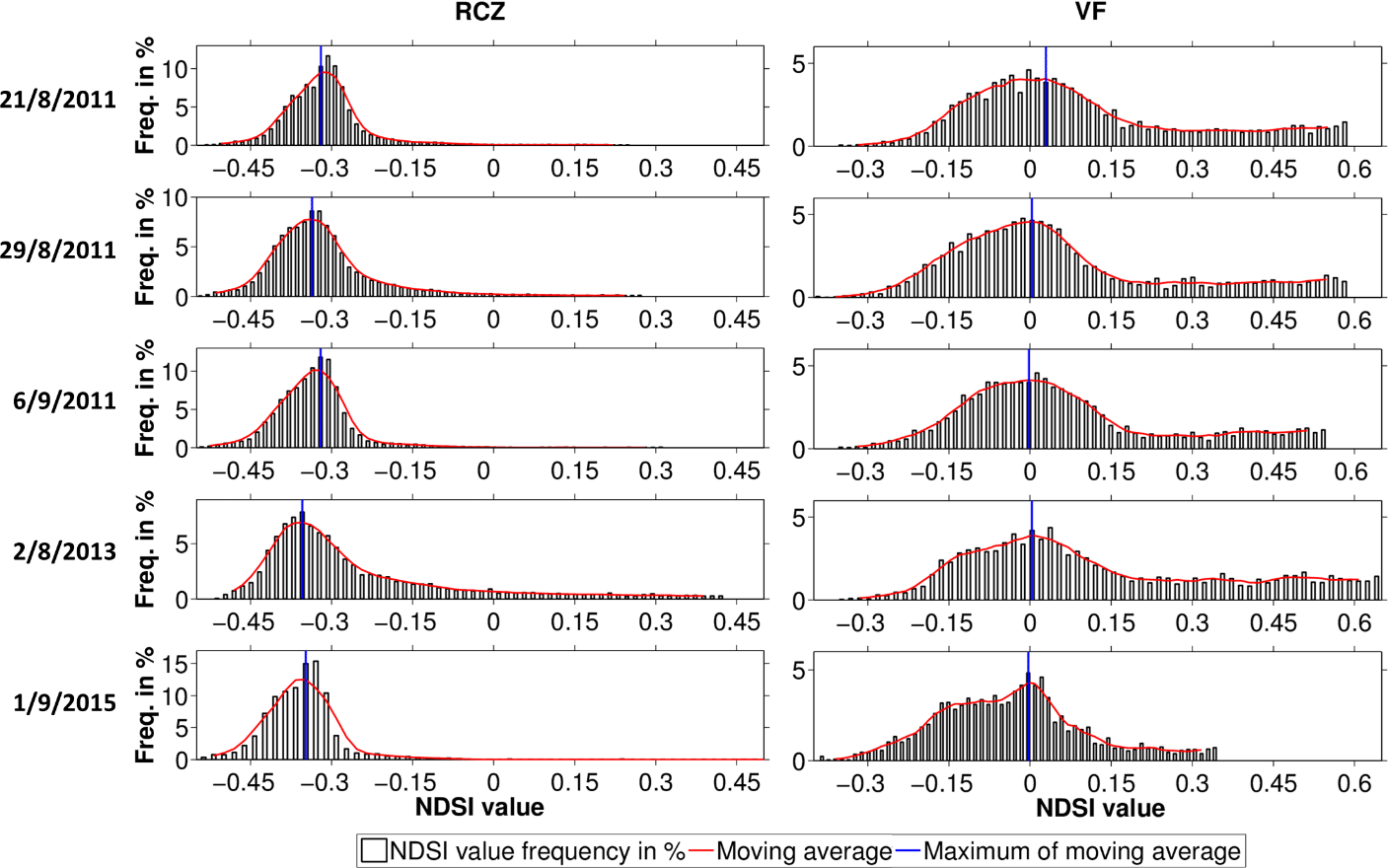
Figure 9Representative NDSI values for the rock surfaces in RCZ and VF catchment are determined using frequency histograms of the snow-free bare rock NDSI values for five summer dates. A smoothed moving average of five histogram classes is shown with red. The maxima of the smoothed histograms are depicted in blue for each catchment and the dates investigated.
The results of the camera-based methods require deeper investigation to analyse if such different NDSIthr values are justifiable. Despite the strong scatter and the resulting low correlation, the differences in the catchment-specific mean NDSIthr levels seem to be systematic (Table 1). Topographic characteristics could be a possible reason. These are similar with respect to elevation, slope and aspect but different for the underlying rock being limestone at RCZ and gneiss at VF. We hence investigated the NDSI values for the snow-free bare rock areas within each catchment. Figure 9 presents frequency histograms of the NDSI for five summer dates. Other seasons were excluded due to the increased probability of fractional snow cover in the Landsat pixels. The tests show that the maximum frequencies after smoothing the histogram are stable for these dates for each catchment. The mean maximum frequency is about −0.34 at RCZ and 0.01 at VF. This corresponds to the spectral behaviour of limestone and gneiss. Limestone is typically lighter than gneiss in the visible range but the reflectance further increases for wavelengths up to 2 µm while it stays similar for a typical gneiss. As the NDSI calculates the difference between the green (0.55 µm) and the mid-infrared wavelength (1.55 µm) in the numerator and uses the sum of these two bands in the denominator, limestone has therefore a negative value and gneiss is around zero. The mean NDSI difference of the rocks at RCZ and VF amounts to about 0.34. This difference is comparable to the mean systematic difference of 0.26 found for the mean calibrated NDSIthr at both sites. It is therefore probable that the different rock types and therefore the background radiation trigger the catchment-specific mean NDSIthr levels which in turn supports the idea of adapting NDSIthr locally.
Next, the effect of the calibrated NDSIthr on the SCA predicted at RCZ and VF is analysed. The differences between the SCA predicted with the standard threshold of 0.4 and those predicted with the Otsu method are small in our study. This can be related to the minor differences between standard NDSIthr and the threshold predicted over Otsu. The absolute differences are 0.05 km2 on average for VF and 0.15 km2 for RCZ. The effects achieved with the photographic method instead are on a level which questions the applicability of the standard threshold for local investigations. The differences in SCA between the products using the calibrated NDSIthr and the standard threshold of 0.4 are calculated using the camera-calibrated SCA as baseline which has shown the highest accuracy of the derived snow cover products when compared to the available photo classifications of PRACTISE (Härer et al., 2016):
The values are between −24.1 % at RCZ and +17.2 % at VF (Fig. 7c) and reveal how different standard and calibrated NDSI-based snow cover maps are on the small scale. The deviations are in general larger at RCZ, where the calibrated NDSI threshold values are mainly below 0.4. This means that the SCA is systematically underestimated when using the standard of 0.4. The lower error at VF compared to the error percentages at RCZ could be related to the generally higher snow-covered area in the VF catchment. These relative differences result in turn in significantly different absolute SCA (standard threshold versus calibrated threshold). Here, the highest differences are 1.09 km2 at RCZ and 1.67 km2 at VF. This is a relevant error margin especially if the small catchment sizes of only 13.1 km2 (RCZ) and 11.5 km2 (VF) are taken into account.
Given this finding and the large variability observed in calibrated NDSIthr, it is obvious that methods which locally calibrate the NDSIthr for a single date and then apply this threshold at multiple dates are probably not a solution. An example is the application of a calibrated threshold of 0.7 at VF to the complete time series in this catchment. We use 0.7 here as stated by Maher et al. (2012) and as it is in the plausible range of the observed NDSI thresholds at VF (0.35 to 0.74). However, when applied to the complete time series, this approach results in a mean absolute error in SCA of 1.26 km2 compared to an average deviation of 0.41 km2 for the standard threshold method. This approach thus might help in some studies where, by chance, an NDSI threshold is found for the calibration date that also describes the other analysis dates well. However, our example shows that the chances are also high that it deteriorates the accuracy compared to the standard threshold method when applied to other dates.
An alternative to the temporally constant threshold methods is a statistical modelling approach fitted to the calibrated NDSIthr. This however requires a solid set of calibration data to adjust the model to the observations at multiple dates. VF hence serves as an example for this approach because of its higher data availability. As stated before a seasonal dynamic in the calibrated NDSIthr could be observed at both sites. A quadratic polynomial model was fitted against the day of year for the calibrated NDSIthr of the years 2010 to 2013 at VF (NDSIvf, Fig. 8). NDSIvf might not exactly reproduce the calibrated thresholds at any time step (r2 = 0.45; RMSE = 0.06), but the evaluation of this simple model for 2014 and 2015 at VF shows a remarkable reduction in the average SCA error from 0.35 km2 when applying the standard threshold of 0.4 down to 0.17 km2. These results are promising. We investigated whether the seasonal behaviour of the calibrated NDSI thresholds can be attributed to the elevation and azimuth angles of the sun. The correlation r between azimuth angle and NDSI is 0.75 for RCZ and 0.42 for VF. For sun elevation, r is 0.77 for RCZ and 0.54 for VF. The found correlation values are significant at the 0.001 level except for the azimuth angle at VF which is significant at the 0.01 level. The sun angles thus explain the seasonal development while the observed variability within the seasons is still unclear. Snow age, grain size, albedo development or other effects might be potential drivers of this behaviour. A detailed investigation of this variability is however beyond this study but will be the subject of future studies.
As not every site is equipped with camera infrastructure, it was also tested if the achieved regression model can be transferred to RCZ while including information about the geology-dependent offset among the average NDSIthr values. Hence, the model is fitted to the complete calibrated NDSIthr time series at VF (r2 = 0.36; RMSE = 0.07) and a term (−0.34) for the systematic mean NDSI difference of the rocks at RCZ and VF is added (NDSIrcz, Fig. 9). The evaluation of NDSIrcz seems to slightly underestimate the calibrated NDSIthr at RCZ. Nevertheless, the quadratic polynomial model accounting for the reflectance differences at different sites results in a significant reduction of snow cover mapping uncertainties of 40 % as the mean SCA error amounts to 0.18 km2 while the application of the standard threshold method causes an average deviation in snow cover of 0.31 km2 in RCZ. Given the assumption that the seasonal dynamic and the correction factor are generally applicable, the presented seasonal model derived from the multi-year use of PRACTISE at a single site is hence not only temporally transferrable: by using information about the spectral properties of the pending rock types without the need for other camera systems, it is also spatially transferrable. This assumption and the transferability of the model is probably only true for high-elevation areas where the atmospheric absorbance is low. Even though the NDSI is an index which reduces the dependence on atmospheric conditions, atmospheric correction might be necessary, in addition to more dynamic approaches that reflect the vegetation growth and senescence over the year for lowland areas. Hence, the approach needs to be further evaluated and developed in future studies with more test sites.
We have now underlined the importance of a locally adapted NDSI threshold calibration for Landsat snow cover maps at the two presented catchments. However, the NDSI threshold dependency detected automatically leads to the question of if threshold adaption is also necessary for coarser-resolution satellite snow cover maps, for example, for a spatial resolution of 500 m or 1 km. Hence, the 30 m Landsat snow cover maps using calibrated and standard NDSI threshold values were aggregated up to 90, 210, 510 and 990 m resolution. Our aggregation experiment of the Landsat snow cover maps for the different NDSI thresholds shows that the SCA deviation between standard and calibrated snow cover maps diminishes for coarser-resolution data in most cases. Figure 10a outlines this error reduction with spatial aggregation for a Landsat 7 scene of Vernagtferner catchment on 16 September 2011. Figure 10b shows the simultaneously captured photograph used for calibration. We however cannot draw an absolute conclusion from Fig. 10a that the difference in snow cover maps among the different thresholds is always reduced with a coarser resolution. The simple reason is that with larger pixel sizes, the number of pixels in the catchment becomes lower and the relative weight of a pixel, being different for different thresholds, becomes larger. Therefore, we decided to investigate at which spatial resolution does the standard and calibrated snow cover maps become identical for the 63 cases investigated in the two catchments. This variable is absolute and thus independent of relative weights and changes with spatial aggregation. The aggregation step to 510 m appears to be of major importance as more than 90 % (58 of 63) of SCA maps become identical at this pixel size. Thus, using the standard threshold of 0.4 instead of the higher NDSI thresholds at VF and the lower NDSI thresholds at RCZ seems to be accurate in most cases with a pixel size of 500 m. For applications at this scale, the positive effect of using camera-calibrated data diminishes and might rarely justify the effort. However, our new method using camera-calibrated data focuses on making use of the higher-resolution satellite data of the Landsat series and of the new Sentinel 2.
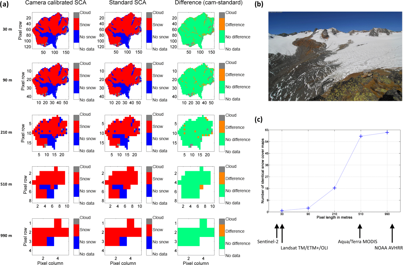
Figure 10At VF, we exemplarily show in (a) the effect of scaling to NDSI-based snow cover products for a Landsat 7 scene on 16 September 2012. The columns from left to right are the camera-calibrated SCA, the standard threshold SCA, and their differences at VF. The different rows show different scaling factors, being 1 (30 m) 3 (90 m), 7 (210 m), 17 (510 m) and 33 (990 m) from the top to the bottom. The concurrent photograph in (b) depicts the snow situation at VF in our example. The analysis of all investigation dates in (c) shows at which pixel size how many of the camera-calibrated and standard threshold snow cover maps become identical. The spatial resolutions of the Sentinel-2, Landsat, MODIS and NOAA AVHRR satellites are outlined for clarity.
The study has revealed that using the standard threshold of 0.4 is adequate for satellite products with a pixel size of 500 m and more. For higher-resolution snow cover mapping, significant improvements in the quality of the snow cover maps can be achieved if a threshold is used which is variable in space and time. The clustering-based segmentation technique of Otsu produces results which are only slightly different from those of the standard threshold of 0.4 and does not indicate a need for a further adaption. However when compared to local images, the resulting differences become obvious and could only be reduced by the presented camera-based technique. The long-term analysis of calibrated NDSIthr at two comparable high-elevation sites has shown that large deviations from the 0.4 standard threshold exist. The calibrated optimal threshold values span a range from 0.15 to 0.74 over the complete time series and can reach a difference of 0.45 between the observation sites at a single date. It was also shown that these differences in NDSIthr lead to significantly different SCA when compared to the standard of 0.4.
The NDSIthr at both sites have similar seasonal dynamics while scattering around different site-specific average values (0.28 at RCZ, 0.57 at VF). The difference between the average threshold values at the two sites could be related to the different reflection properties of the rock types in the investigation areas (limestone at RCZ and gneiss at VF). The overall correlation coefficient between NDSIthr of both sites is low (r = 0.17). This prohibits the general use of one catchment's calibrated threshold values in another catchment of the same satellite scene.
In view of the validity of the standard threshold of 0.4 at the local scale it was found that relative SCA error margins of up to 24.1 % were found for the standard threshold method when using 30m Landsat products. This is critical for any snow cover mapping application and especially for model evaluation studies. We hence conclude that the application of a fixed NDSI threshold can lead to large uncertainties in the resulting snow cover products at least at the local scale. Consequently, local studies must account for the NDSIthr variability in space and time in order to guarantee high-accuracy snow cover products. However, when studies are carried out with sensors with a pixel size of 500 m or greater, the advantage of a location-dependent NDSIthr vanishes.
It was shown that site-specific single-date adaptations of the NDSIthr also do not lead to resilient results. The uncertainty introduced by a single measurement is not quantifiable and can lead to results worse than that achieved by using the standard value of 0.4. A quantitative calibration or visual derivation of the NDSIthr for a single date and its application to other dates is therefore inappropriate.
The approximation of the NDSIthr over a simple seasonal model fitted to the calibrated NDSIthr at the respective site has shown improvements instead. The achieved model was able to reduce the error in the SCA prediction by 50 % when compared to the standard threshold method. Nevertheless, a fundamental data pool of in situ information covering the dynamic over the year and the range of possible NDSIthr within a season is needed for calculating this relation. Finally, it was shown that the fitted model parameters are also spatially transferable if an additional term accounts for the background radiation of the different rock types. This is possible without in situ measurements by utilizing the constant NDSI differences of the rock surface in the respective catchments. However, this needs to be further tested at more sites. Future studies will hence use the existent webcam infrastructure in the European Alps as well as camera systems installed worldwide at the INARCH network sites (Pomeroy et al., 2015) for the generation of numerous calibrated NDSIthr. The observed threshold values will serve as an operational source for applicable NDSIthr and will allow for the evaluation of the presented temporally and spatially variable prediction approach of NDSIthr. In the case of a successful evaluation, the presented scheme allows for objective and reproducible derivation of the NDSIthr value for any given satellite scene. This is a large advantage as, until now, the threshold is often set intuitively or assumed to be constant, which neither conforms to the complexity of the models evaluated on basis of NDSI-based snow cover maps nor to the needs of the models which assimilate these maps.
Relevant data can be made available upon request to the authors.
The authors declare that they have no conflict of interest.
This work was funded by the Austrian Science Fund (I 2142-N29), the doctoral
scholarship program of the German Federal Environmental Foundation (DBU) and
the Helmholtz Research School Mechanisms and Interactions of Climate Change
in Mountain Regions (MICMoR), and has additionally received a fundamental
support of the Environmental Research Station Schneefernerhaus (UFS) as
part of the Virtual Alpine Observatory (VAO). The Commission for
Glaciology of the Bavarian Academy of Sciences and Humanities kindly
provided Vernagtferner data. We want to thank the crew of the UFS (Markus Neumann,
Till Rehm and Hannes Hiergeist) for supporting this piece of
research by hosting the authors and maintaining the camera system. Thomas Werz
and Michael Weber also supported the research by periodically
maintaining the camera system. Finally, we want to thank the editor Guillaume Chambon, and the reviewers Simon Cascoin and Nick Rutter
for their useful
comments and suggestions on the manuscript.
Edited by: Guillaume Chambon
Reviewed by: Nick Rutter and Simon Gascoin
Abermann, J., Kuhn, M., and Fischer, A.: A reconstruction of annual mass balances of Austria's glaciers from 1969 to 1998, Ann. Glaciol., 52, 127–134, https://doi.org/10.3189/172756411799096259, 2011.
Agosta, C., Fettweis, X., and Datta, R.: Evaluation of the CMIP5 models in the aim of regional modelling of the Antarctic surface mass balance, The Cryosphere, 9, 2311–2321, https://doi.org/10.5194/tc-9-2311-2015, 2015.
Aronica, G., Bates, P. D., and Horritt, M. S.: Assessing the uncertainty in distributed model predictions using observed binary pattern information within GLUE, Hydrol. Process., 16, 2001–2016, https://doi.org/10.1002/hyp.398, 2002.
Bernhardt, M. and Schulz, K.: SnowSlide: A simple routine for calculating gravitational snow transport, Geophys. Res. Lett., 37, L11502, https://doi.org/10.1029/2010GL043086, 2010.
Bernhardt, M., Schulz, K., Liston, G. E., and Zängl, G.: The influence of lateral snow redistribution processes on snow melt and sublimation in alpine regions, J. Hydrol., 424–425, 196–206, https://doi.org/10.1016/j.jhydrol.2012.01.001, 2012.
Bernhardt, M., Härer, S., Jacobeit, J., Wetzel, K. F., and Schulz, K.: The Virtual Alpine Observatory – research focus Alpine hydrology, Hydrol. Wasserbewirts., 58, 241–243, 2014.
Bernhardt, M., Schulz, K., and Pomeroy, J.: The International Network for Alpine Research Catchment Hydrology. A new GEWEX crosscutting Project, Hydrol. Wasserbewirts., 59, 190–191, 2015.
Burns, P. and Nolin, A.: Using atmospherically-corrected Landsat imagery to measure glacier area change in the Cordillera Blanca, Peru from 1987 to 2010, Remote Sens. Environ., 140, 165–178, https://doi.org/10.1016/j.rse.2013.08.026, 2014.
Butt, M. J.,and Bilal, M.: Application of snowmelt runoff model for water resource management, Hydrol. Process., 25, 3735–3747, https://doi.org/10.1002/hyp.8099, 2011.
Chaponnière, A., Maisongradne, P., Duchemin, B., Hanich, L., Boulet, G., Escadal, R., and Elouaddat, S.: A combined high and low spatial resolution approach for mapping snow covered areas in the Atlas mountains, Int. J. Remote Sens., 26, 2755–2777, https://doi.org/10.1080/01431160500117758, 2005.
Deb, D., Butcher, J., and Srinivasan, R.: Projected Hydrologic Changes Under Mid-21st Century Climatic Conditions in a Sub-arctic Watershed, Water Resour. Manage., 29, 1467–1487, https://doi.org/10.1007/s11269-014-0887-5, 2015.
Dee, D. P., Uppala, S. M., Simmons, A. J., Berrisford, P., Poli, P., Kobayashi, S., Andrae, U., Balmaseda, M. A., Balsamo, G., Bauer, P., Bechtold, P., Beljaars, A. C. M., van de Berg, L., Bidlot, J., Bormann, N., Delsol, C., Dragani, R., Fuentes, M., Geer, A. J., Haimberger, L., Healy, S. B., Hersbach, H., Holm, E. V., Isaksen, L., Kallberg, P., Koehler, M., Matricardi, M., McNally, A. P., Monge-Sanz, B. M., Morcrette, J.-J., Park, B.-K., Peubey, C., de Rosnay, P., Tavolato, C., Thepaut, J.-N., and Vitart, F.: The ERA-Interim reanalysis: configuration and performance of the data assimilation system, Q. J. Roy. Meteorol. Soc., 137, 553–597, https://doi.org/10.1002/qj.828, 2011.
Dozier, J.: Snow reflectance from LANDSAT-4 Thematic Mapper, IEEE T. Geosci. Remote, GE-22, 323–328, https://doi.org/10.1109/TGRS.1984.350628, 1984.
Dozier, J.: Spectral Signature of Alpine Snow Cover from the Landsat Thematic Mapper, Remote Sens. Environ., 28, 9–22, https://doi.org/10.1016/0034-4257(89)90101-6, 1989.
Drusch, M., Vasiljevic, D., and Viterbo, P.: ECMWF's global snow analysis: Assessment and revision based on satellite observations, J. Appl. Meteorol., 43, 1282–1294, https://doi.org/10.1175/1520-0450(2004)043<1282:EGSAAA>2.0.CO;2, 2004.
Dutra, E., Viterbo, P., Miranda, P. M. A., and Balsamo, G.: Complexity of Snow Schemes in a Climate Model and Its Impact on Surface Energy and Hydrology, J. Hydrometeorol., 13, 521–538, https://doi.org/10.1175/JHM-D-11-072.1, 2012.
Dyurgerov, M.: Mountain and subpolar glaciers show an increase in sensitivity to climate warming and intensification of the water cycle, J. Hydrol., 282, 164–176, https://doi.org/10.1016/S0022-1694(03)00254-3, 2003.
Hall, D. K. and Riggs, G. A.: Accuracy assessment of the MODIS snow products, Hydrol. Process., 21, 1534–1547, https://doi.org/10.1002/hyp.6715, 2007.
Hall, D. K., Foster, J. L., Salomonson, V. V., Klein, A. G., and Chien, J. Y. L.: Development of a technique to assess snow-cover mapping errors from space, IEEE T. Geosci. Remote, 39, 432–438, https://doi.org/10.1109/36.905251, 2001.
Hall, D. K., Riggs, G. A., Salomonson, V. V., DiGirolamo, N. E., and Bayr, K. J.: MODIS snow-cover products, Remote Sens. Environ., 83, 181–194, https://doi.org/10.1016/S0034-4257(02)00095-0, 2002.
Härer, S., Bernhardt, M., Corripio, J. G., and Schulz, K.: PRACTISE – Photo Rectification And ClassificaTIon SoftwarE (V.1.0), Geosci. Model Dev., 6, 837–848, https://doi.org/10.5194/gmd-6-837-2013, 2013.
Härer, S., Bernhardt, M., and Schulz, K.: PRACTISE – Photo Rectification And ClassificaTIon SoftwarE (V.2.1), Geosci. Model Dev., 9, 307–321, https://doi.org/10.5194/gmd-9-307-2016, 2016.
Homan, J. W., Luce, C. H., McNamara, J. P., and Glenn, N. F.: Improvement of distributed snowmelt energy balance modeling with MODIS-based NDSI-derived fractional snow-covered area data, Hydrol. Process., 25, 650–660, https://doi.org/10.1002/hyp.7857, 2011.
Kyle, H. L., Curran, R. J., Barnes, W. L., and Escoe, D.: A cloud physics radiometer, in: 3rd Conference on Atmospheric Radiation, American Meteorological Society, 28–30 June 1978, Davis, California, p. 107, 1978.
Liston, G. E.: Representing subgrid snow cover heterogeneities in regional and global models, J. Climate, 17, 1381–1397, https://doi.org/10.1175/1520-0442(2004)017<1381:RSSCHI>2.0.CO;2, 2004.
Maher, A. I., Treitz, P. M., and Ferguson, M. A. D.: Can Landsat data detect variations in snow cover within habitats of arctic ungulates?, Wildlife Biol., 18, 75–87, https://doi.org/10.2981/11-055, 2012.
Mankin, J. S. and Diffenbaugh, N. S.: Influence of temperature and precipitation variability on near-term snow trends, Clim. Dynam., 45, 1099-1116, https://doi.org/10.1007/s00382-014-2357-4, 2015.
Maussion, F., Scherer, D., Finkelnburg, R., Richters, J., Yang, W., and Yao, T.: WRF simulation of a precipitation event over the Tibetan Plateau, China – an assessment using remote sensing and ground observations, Hydrol. Earth Syst. Sci., 15, 1795–1817, https://doi.org/10.5194/hess-15-1795-2011, 2011.
Mayr, E., Hagg, W., Mayer, C., and Braun, L.: Calibrating a spatially distributed conceptual hydrological model using runoff, annual mass balance and winter mass balance, J. Hydrol., 478, 40–49, https://doi.org/10.1016/j.jhydrol.2012.11.035, 2013.
Otsu, N.: Threshold Selection Method from Gray-Level Histograms, IEEE T. Syst. Man. Cyb., 9, 62–66, https://doi.org/10.1109/Tsmc.1979.4310076, 1979.
Painter, T. H., Rittger, K., McKenzie, C., Slaughter, P., Davis R. E., and Dozier, J.: Retrieval of subpixel snow covered area, grain size, and albedo from MODIS, Remote Sens. Environ., 113, 868–879, https://doi.org/10.1016/j.rse.2009.01.001, 2009.
Pomeroy, J., Bernhardt, M., and Marks, D.: Research network to track alpine water, Nature, 521, 32–32 https://doi.org/10.1038/521032c, 2015.
Racoviteanu, A. E., Paul, F., Raup, B., Khalsa, S. J. S., and Armstrong, R.: Challenges and recommendations in mapping of glacier parameters from space: results of the 2008 Global Land Ice Measurements from Space (GLIMS) workshop, Boulder, Colorado, USA, Ann. Glaciol., 50, 53–69, https://doi.org/10.3189/172756410790595804, 2009.
Rangwala, I., Miller, J. R., Russell, G. L., and Xu, M.: Using a global climate model to evaluate the influences of water vapor, snow cover and atmospheric aerosol on warming in the Tibetan Plateau during the twenty-first century, Clim. Dynam., 34, 859–872, https://doi.org/10.1007/s00382-009-0564-1, 2010.
Rouse Jr., J., Haas, R. H., Schell, J. A., and Deering, D. W.: Monitoring vegetation systems in the Great Plains with ERTS, in: 3rd Earth Resources Technology Satellite-1 Symposium – Vol. I: Technical Presentations, NASA SP-351, NASA, Washington, USA, 309–317, 1974.
Salvatori, R., Plini, P., Giusto, M., Valt, M., Salzano, R., Montagnoli, M., Cagnati, A., Crepaz, G., and Sigismondi, D.: Snow cover monitoring with images from digital camera systems, Ital. J. Remote Sens., 43, 137–145, https://doi.org/10.5721/ItJRS201143211, 2011.
Sankey, T., Donald, J., Mcvay, J., Ashley, M., O'Donnell, F., Lopez, S. M., and Springer, A.: Multi-scale analysis of snow dynamics at the southern margin of the North American continental snow distribution, Remote Sens. Environ., 169, 307–319, https://doi.org/10.1016/j.rse.2015.08.028, 2015.
Santini, M. and di Paola, A.: Changes in the world rivers' discharge projected from an updated high resolution dataset of current and future climate zones, J. Hydrol., 531, 768–780, https://doi.org/10.1016/j.jhydrol.2015.10.050, 2015.
Silverio, W. and Jaquet, J. M.: Prototype land-cover mapping of the Huascaran Biosphere Reserve (Peru) using a digital elevation model, and the NDSI and NDVI indices, J. Appl. Remote Sens., 3, 033516, https://doi.org/10.1117/1.3106599, 2009.
Sirguey, P., Mathieu, R., and Arnaud, Y.: Subpixel monitoring of the seasonal snow cover with MODIS at 250 m spatial resolution in the Southern Alps of New Zealand: Methodology and accuracy assessment, Remote Sens. Environ., 113, 160–181, https://doi.org/10.1016/j.rse.2008.09.008, 2009.
Takata, K., Emori, S., and Watanabe, T.: Development of the minimal advanced treatments of surface interaction and runoff, Global Planet. Change, 38, 209–222, https://doi.org/10.1016/S0921-8181(03)00030-4, 2003.
Tekeli, A. E., Akyurek, Z., Sorman, A. A., Sensoy, A., and Sorman, A. U.: Using MODIS snow cover maps in modeling snowmelt runoff process in the eastern part of Turkey, Remote Sens. Environ., 97, 216–230, https://doi.org/10.1016/j.rse.2005.03.013, 2005.
Tennant, C. J., Crosby, B. T., and Godsey, S. E.: Elevation-dependent responses of streamflow to climate warming, Hydrol. Process., 29, 991–1001, https://doi.org/10.1002/hyp.10203, 2015.
Thirel, G., Salamon, P., Burek, P., and Kalas, M.: Assimilation of MODIS Snow Cover Area Data in a Distributed Hydrological Model Using the Particle Filter, Remote Sens., 5, 5825–5850, https://doi.org/10.3390/rs5115825, 2013.
Tucker, C. J.: Red and photographic infrared linear combinations for monitoring vegetation, Remote Sens. Environ., 8, 127–150, https://doi.org/10.1016/0034-4257(79)90013-0, 1979.
Vavrus, S., Philippon-Berthier, G., Kutzbach, J. E., and Ruddiman, W. F.: The role of GCM resolution in simulating glacial inception, Holocene, 21, 819–830, https://doi.org/10.1177/0959683610394882, 2011.
Viviroli, D., Archer, D. R., Buytaert, W., Fowler, H. J., Greenwood, G. B., Hamlet, A. F., Huang, Y., Koboltschnig, G., Litaor, M. I., Lopez-Moreno, J. I., Lorentz, S., Schaedler, B., Schreier, H., Schwaiger, K., Vuille, M., and Woods, R.: Climate change and mountain water resources: overview and recommendations for research, management and policy, Hydrol. Earth Syst. Sci., 15, 471–504, https://doi.org/10.5194/hess-15-471-2011, 2011.
Warscher, M., Strasser, U., Kraller, G., Marke, T., Franz, H., and Kunstmann, H.: Performance of complex snow cover descriptions in a distributed hydrological model system: A case study for the high Alpine terrain of the Berchtesgaden Alps, Water Resour. Res., 49, 2619–2637, https://doi.org/10.1002/wrcr.20219, 2013.
Weber, M., Bernhardt, M., Pomeroy, J. W., Fang, X., Härer, S., and Schulz, K.: Description of current and future snow processes in a small basin in the Bavarian Alps, Environ. Earth Sci., 75, 1223, https://doi.org/10.1007/s12665-016-6027-1, 2016.
Yin, D., Gao, X., Chen, X., Shao, Y., and Chen, J.: Comparison of automatic thresholding methods for snow-cover mapping using Landsat TM imagery, Int. J. Remote Sens., 34, 6529–6538, https://doi.org/10.1080/01431161.2013.803631, 2013.
Zhu, Z., Wang, S., and Woodcock, C. E.: Improvement and expansion of the Fmask algorithm: cloud, cloud shadow, and snow detection for Landsats 4–7, 8, and Sentinel 2 images, Remote Sens. Environ., 159, 269–277, https://doi.org/10.1016/j.rse.2014.12.014, 2015.