the Creative Commons Attribution 4.0 License.
the Creative Commons Attribution 4.0 License.
 | 12 Apr 2018
Estimating the snow water equivalent on a glacierized high elevation site (Forni Glacier, Italy)
Antonella Senese
Maurizio Maugeri
Eraldo Meraldi
Gian Pietro Verza
Roberto Sergio Azzoni
Chiara Compostella
Guglielmina Diolaiuti
We present and compare 11 years of snow data (snow depth and snow water equivalent, SWE) measured by an automatic weather station (AWS) and corroborated by data from field campaigns on the Forni Glacier in Italy. The aim of the analysis is to estimate the SWE of new snowfall and the annual SWE peak based on the average density of the new snow at the site (corresponding to the snowfall during the standard observation period of 24 h) and automated snow depth measurements. The results indicate that the daily SR50 sonic ranger measurements and the available snow pit data can be used to estimate the mean new snow density value at the site, with an error of ±6 kg m−3. Once the new snow density is known, the sonic ranger makes it possible to derive SWE values with an RMSE of 45 mm water equivalent (if compared with snow pillow measurements), which turns out to be about 8 % of the total SWE yearly average. Therefore, the methodology we present is interesting for remote locations such as glaciers or high alpine regions, as it makes it possible to estimate the total SWE using a relatively inexpensive, low-power, low-maintenance, and reliable instrument such as the sonic ranger.
- Article
(5046 KB) - Full-text XML
- BibTeX
- EndNote


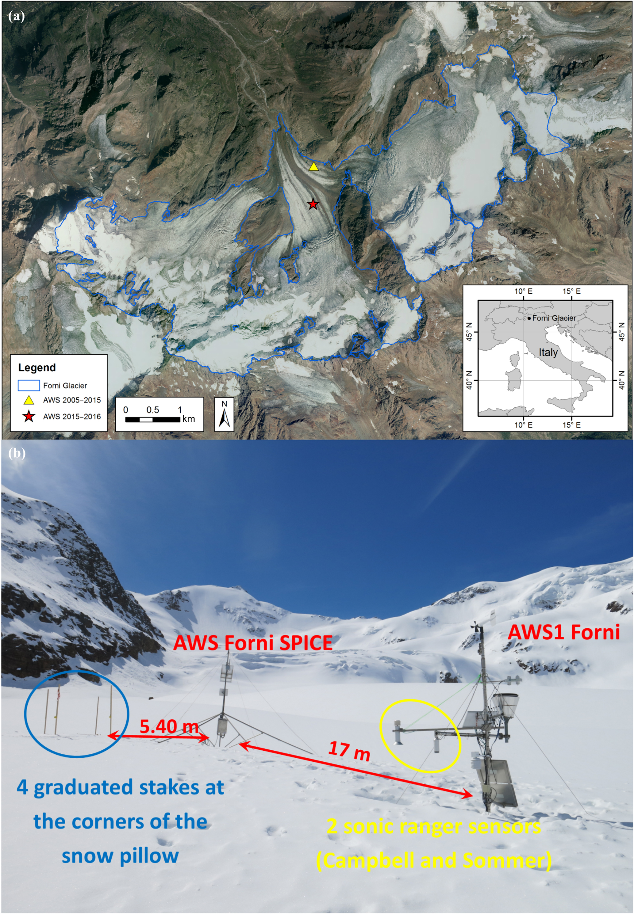
Figure 1(a) The study site. The yellow triangle indicates the location of the AWS1 Forni and the Forni AWS SPICE until November 2015. The red star refers to the actual location after securing the stations. (b) AWS1 Forni (on the right) and AWS Forni SPICE (on the left) photographed from the northeast on 6 May 2014 (immediately after the installation of the AWS Forni SPICE). The distances between the stations are shown.
The study of the spatial and temporal variability of water resources deriving from snowmelt (i.e., snow water equivalent, SWE) is very important for estimating the water balance at the catchment scale. Many areas depend on this freshwater reservoir for civil use, irrigation, and hydropower, so they need an accurate and updated evaluation of SWE magnitude and variability. In addition, a correct SWE assessment also supports early strategies for managing and preventing hydro-meteorological risks (e.g., flood forecasting, avalanche forecasting). New snow-density evaluation is also important for snowfall forecasting based on orographic precipitation models (Judson and Doesken, 2000; Roebber et al., 2003), estimation of avalanche hazards (Perla, 1970; LaChapelle, 1980; Ferguson et al., 1990; McClung and Schaerer, 1993), snowdrift forecasting, as an input parameter in the snow accumulation algorithm (Super and Holroyd, 1997), and general snow science research.
In high mountain areas, however, often only snowfall measurements are available: a correct evaluation of new snow density (ρnew snow) is therefore needed to calculate the SWE. Since new snow density is site specific and depends on atmospheric and surface conditions, the main aim of this study is to investigate the magnitude and rates of variations in ρnew snow and to understand how an incorrect assessment of this variable may affect the estimation of the SWE. This was possible by means of systematic manual and automatic measurements carried out at the surface of the Forni Glacier (Stelvio National Park, Italian Alps; Fig. 1a and b). Since 2005, an automatic weather station (AWS1 Forni) has been acquiring snow data at the glacier surface, in addition to snow pit measurements of snow depth and SWE carried out by expert personnel (Citterio et al., 2007; Senese et al., 2012a, b, 2014). The snow data thus acquired refer to snowfall or new snow (i.e., depth of freshly fallen snow deposited over a standard observation period, generally 24 h; see WMO, 2008; Fierz et al., 2009) and to snow depth (i.e., the total depth of snow on the ground at the time of observation; see WMO, 2008).
In general, precipitation can be measured mechanically, optically, by capacitive sensing, and by radar. Some examples of available sensors are the heated tipping bucket rain gauge (as precipitation is collected and melted in the gauge's funnel, water is directed to a tipping bucket mechanism adjusted to tip and dump when a threshold volume of water is collected), the heated weighing gauge (the weight of water collected is measured as a function of time and converted to rainfall depth), and the disdrometer (measuring the drop size distribution and the velocity of falling hydrometeors). For catchment-type precipitation sensors, the catch efficiency of solid precipitation needs to be considered for the correct measurement of new snow. For the Solid Precipitation Intercomparison Experiment (1989–1993), the International Organizing Committee designated the Double Fence Intercomparison Reference (DFIR) as the reference for intercomparison (WMO/TD-872, 1998, Sect. 2.2.2). Even if all these methods mentioned provide accurate measurements, it is very difficult to utilize some of them in remote areas like a glacier site. For this reason, at the Forni Glacier, snow data have been acquired by means of sonic ranger and snow pillow instrumentations, without wind shielding.
For estimating SWE from snow depth measurements alone, correct new snow density estimate is crucial. Following Roebber et al. (2003), new snow density is often assumed to conform to the 10-to-1 rule: the snow ratio, defined as the density of water (1000 kg m−3) to the density of new snow (assumed to be 100 kg m−3), is 10 : 1. As noted by Judson and Doesken (2000), the 10-to-1 rule appears to originate from the results of a nineteenth-century Canadian study. More comprehensive measurements (e.g., Currie, 1947; LaChapelle, 1962; Power et al., 1964; Super and Holroyd, 1997; Judson and Doesken, 2000) have established that this rule is an inadequate characterization of the true range of new snow densities. Indeed, they can vary from 10 kg m−3 to approximately 350 kg m−3 (Roebber et al., 2003). Bocchiola and Rosso (2007) report a similar range for the Central Italian Alps with values varying from 30 to 480 kg m−3, and an average sample value of 123 kg m−3. The lower bound of new snow density is usually about 50 kg m−3 (Gray, 1979; Anderson and Crawford, 1964). Judson and Doesken (2000) found densities of new snow observed from six sheltered avalanche sites in the Central Rocky Mountains to range from 10 to 257 kg m−3, and average densities at each site based on 4 years of daily observations ranged from 72 to 103 kg m−3. Roebber et al. (2003) found that the 10-to-1 rule may be modified slightly to 12 to 1 or doubled to 20 to 1, depending on the mean or median climatological value of new snow density at a particular station (e.g., Currie, 1947; Super and Holroyd, 1997). Following Pahaut (1975), the new snow density ranges from 20 to 200 kg m−3 and increases with wind speed and air temperature. Wetzel and Martin (2001) analyzed all empirical techniques evolved in the absence of explicit snow-density forecasts. As argued in Schultz et al. (2002), however, these techniques might be not fully adequate and the accuracy should be carefully verified for a large variety of events.
New snow density is regulated by (i) in-cloud processes that affect the shape and size of ice crystal growth, (ii) sub-cloud thermodynamic stratification through which the ice crystals fall (since the low-level air temperature and relative humidity regulate the processes of sublimation or melting of a snowflake), and (iii) ground-level compaction due to prevailing weather conditions and snowpack metamorphism. Understanding how these processes affect new snow density is difficult because direct observations of cloud microphysical processes, thermodynamic profiles, and surface measurements are often unavailable.
Cloud microphysical research indicates that many factors contribute to the final structure of an ice crystal. The shape of the ice crystal is determined by the environment in which the ice crystal grows: pure dendrites have the lowest density (Power et al., 1964), although the variation in the density of dendritic aggregates is large (from approximately 5 to 100 kg m−3, Magono and Nakamura, 1965; Passarelli and Srivastava, 1979). Numerous observational studies over decades clearly demonstrate that the density varies inversely with size (Magono and Nakamura, 1965; Holroyd, 1971; Muramoto et al., 1995; Fabry and Szyrmer, 1999; Heymsfield et al., 2004; Brandes et al., 2007). The crystal size is related to the ratio between ice and air (Roebber et al., 2003): large dendritic crystals can occupy much empty air space, whereas smaller crystals can pack together into a denser assemblage. In addition, as an ice crystal falls, it passes through varying thermodynamic and moisture conditions. Then, the ultimate shape and size of crystals depend on factors that affect the growth rate and are a combination of various growth modes (e.g., Pruppacher and Klett, 1997).
To contribute to the understanding of all the above topics, in this paper we discuss and compare all the available snow data measured at the Forni Glacier surface in the last decade to (i) suggest the most suitable measurement system for evaluating SWE at the glacier surface (i.e., snow pillow, sonic ranger, snow pit, or snow weighing tube); (ii) assess the capability to obtain SWE values from the depth measurements and their accuracies; (iii) check the validity of the ρnew snow value previously found (i.e., 140 kg m−3; see Senese et al., 2014) in order to support SWE computation; and (iv) evaluate effects and impacts of uncertainties in the ρnew snow value in relation to the derived SWE amount.
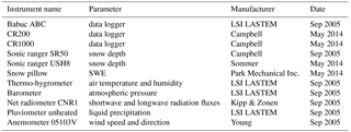
Table 1Instrumentation at the Forni Glacier with instrument name, measured parameter, manufacturer, and starting date.
The Forni Glacier (one of the largest glaciers in Italy) is a Site of Community Importance (SCI, code IT2040014) located inside an extensive natural protected area (Stelvio National Park). It is a wide valley glacier (ca. 11.34 km2, D'Agata et al., 2014), covering an elevation range from 2600 to 3670 m a.s.l.
The first Italian supraglacial station (AWS1 Forni; Fig. 1b) was set up on 26 September 2005 at the lower sector of the eastern tongue of Forni Glacier (Citterio et al., 2007; Senese et al., 2012a, b, 2014, 2016). The WGS84 coordinates of AWS1 Forni were 46∘23′56.0 N, 10∘35′25.2 E; 2631 m a.s.l. (Fig. 1a, yellow triangle). The second station (AWS Forni SPICE; Fig. 1b) was set up on 6 May 2014 close to AWS1 Forni (at a distance of about 17 m). Due to the formation of ring faults, in November 2015 both AWSs were moved to the Forni Glacier central tongue (46∘23′42.40 N and 10∘35′24.20 E, at an elevation of 2675 m a.s.l., the red star in Fig. 1a). Ring faults are a series of circular or semicircular fractures with stepwise subsidence (caused by englacial or subglacial meltwater) that could compromise the stability of the stations because they could create voids at the ice-bedrock interface and eventually cause the collapse of cavity roofs (Azzoni et al., 2017; Fugazza et al., 2017).
The main challenges in installing and managing Forni AWSs were due to the fact that the site is located on the surface of an Alpine glacier, not always accessible, especially during wintertime when skis and skins are needed on the steep and narrow path, and avalanches can occur. Moreover, the glacier is a dynamic body (moving up to 20–30 m yr−1, Urbini et al., 2017) and its surface also features a well-developed roughness due to ice melting, flowing meltwater, differential ablation, and opening crevasses (Diolaiuti and Smiraglia, 2010; Smiraglia and Diolaiuti, 2011). In addition, the power to be supplied to instruments and sensors is only provided by solar panels and lead–gel batteries. A thorough and accurate analysis of instruments and devices (i.e., energy supply required, performance and efficiency operation at low temperatures, noise in measuring due to ice flow, etc.) was required before their installation on the supraglacial AWSs to avoid interruptions in data acquisition and storage.
AWS1 Forni is equipped with sensors for measuring air temperature and humidity (a naturally ventilated shielded sensor), wind speed and direction, air pressure, and the four components of the radiation budget (longwave and shortwave, both incoming and outgoing fluxes). Liquid precipitation is measured by means of an unheated precipitation gauge, and snow depth by means of the Campbell SR50 sonic ranger (Table 1; see also Senese et al., 2012a).
AWS Forni SPICE is equipped with a snow pillow (Park Mechanical steel snow pillow, 150 × 120 × 1.5 cm) and a barometer (STS ATM.1ST) for measuring the SWE (Table 1, Beaumont, 1965). The measured air pressure permits calibration of the output values recorded by the snow pillow. The snow pillow pressure gauge is a device similar to a large air or water mattress filled with antifreeze. As snow is deposited on this gauge, the pressure increase is related to the accumulating mass and thus to SWE. On the mast, an automated camera was installed to photograph the four graduated stakes located at the corners of the snow pillow (Fig. 1b) in order to observe the snow depth. When the snow pillow was installed at AWS Forni SPICE, a second sonic ranger (Sommer USH8) was installed at AWS1 Forni.
The entire systems of both AWS1 Forni and AWS Forni SPICE are supported by four-leg stainless steel masts (5 and 6 m high, respectively) standing on the ice surface. In this way, the AWSs stand freely on the ice, and move together with the melting surface during summer (with a mean ice thickness variation of about 4 m yr−1).
The automated instruments are sampled every 60 s. The SR50 sonic ranger, wind sensor, and barometer samples are averaged every 60 min. The air temperature, relative humidity, solar and infrared radiation, and liquid precipitation sample are averaged every 30 min. The USH8 sonic ranger and snow pillow sample are averaged every 10 min. All data are recorded in a flash memory card, including the basic distribution parameters (minimum, mean, maximum, and standard deviation values).
The long sequence of meteorological and glaciological data permitted the introduction of the AWS1 Forni into the SPICE (Solid Precipitation Intercomparison Experiment) project managed and promoted by the WMO (World Meteorological Organization; Nitu et al., 2012) and the CryoNet project (Global Cryosphere Watch's core project, promoted by the WMO; Key et al., 2015).
Snow data at the Forni Glacier have been acquired by means of (i) a Campbell SR50 sonic ranger since October 2005 (snow depth data), (ii) manual snow pits since January 2006 (snow depth and SWE data), (iii) a Sommer USH8 sonic ranger since May 2014 (snow depth data), (iv) a Park Mechanical SS-6048 snow pillow since May 2014 (SWE data) and (v) a manual snow weighing tube (Enel-Valtecne) since May 2014 (snow depth and SWE data). These measurements were made at the two AWSs: AWS1 Forni and AWS Forni SPICE.
Comparing the datasets from the Campbell and Sommer sensors, very good agreement is found (r=0.93). This means that both sensors worked correctly. In addition, from 2015 onwards, the double snow depth datasets could mean better data for the SWE estimate.
In addition to the measurements recorded by the AWSs, since winter 2005–2006, personnel from the Centro Nivo-Meteorologico (namely of CNM Bormio-ARPA Lombardia) of the Lombardy Regional Agency for the Environment have periodically used snow pits (performed according to the AINEVA protocol; see also Senese et al., 2014) in order to estimate snow depth and SWE (in millimeters water equivalent, w.e.). In particular, for each snow pit j, the thickness (hij) and the density (ρij) of each snow layer (i) are measured for determining its SWE, and then the total SWEsnow-pit-j of the entire snow cover (n layers) is obtained:
where ρwater is water density. As noted in a previous study (Senese et al., 2014), the date when the snow pit is dug is very important for not underestimating the actual accumulation. For this reason, we considered only the snow pits excavated before the beginning of snow ablation. In fact, whenever ablation occurs, successive SWE values derived from snow pits show a decreasing trend (i.e., they are affected by mass losses).
The snow pit SWE data were then used, together with the corresponding total new snow derived from sonic ranger readings, to estimate the site average ρnew snow, in order to update the value of 140 kg m−3 that was found in a previous study of data of the same site covering the period 2005–2009 (Senese et al., 2012a). Specifically, for each snow pit j, the corresponding total new snow was first determined by
where m is the total number of days with snowfall in the period corresponding to snow pit j, and Δhtj corresponds to the depth of new snow on day t. Indeed, the new snow is defined as the depth of freshly fallen snow deposited over a standard observation period, generally 24 h (see WMO, 2008; Fierz et al., 2009). In particular, we considered the hourly snow depth values recorded by the sonic ranger in a day and we calculated the difference between the last and the first reading. Whenever this difference is positive (at least 1 cm), it corresponds to a new snowfall. All data are subject to strict quality control to avoid under- or over-measurements, to remove outliers and nonsense values, and to filter possible noise. is therefore the total new snow measured by the Campbell SR50 from the beginning of the accumulation period to the date of the snow pit survey. Obviously, this value is higher than the snow depth recorded by the sonic ranger when the snow pit is dug, due to settling.
The average site ρnew snow was then determined as
where j identifies a given snow pit and the corresponding total new snow, and the sum extends over all k-available snow pits. Instead of a mere average of ρnew snow values obtained from individual snow pit surveys, this relation gives more weight to snow pits with a higher SWEsnow-pit amount.
The SWESR (from sonic ranger data) for each day (t) was then estimated by
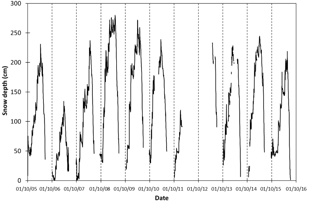
Figure 2Daily snow depth measured by the Campbell SR-50 sonic ranger at the AWS1 Forni from 1 October 2005 to 30 September 2016. The dates shown are dd/mm/yy.
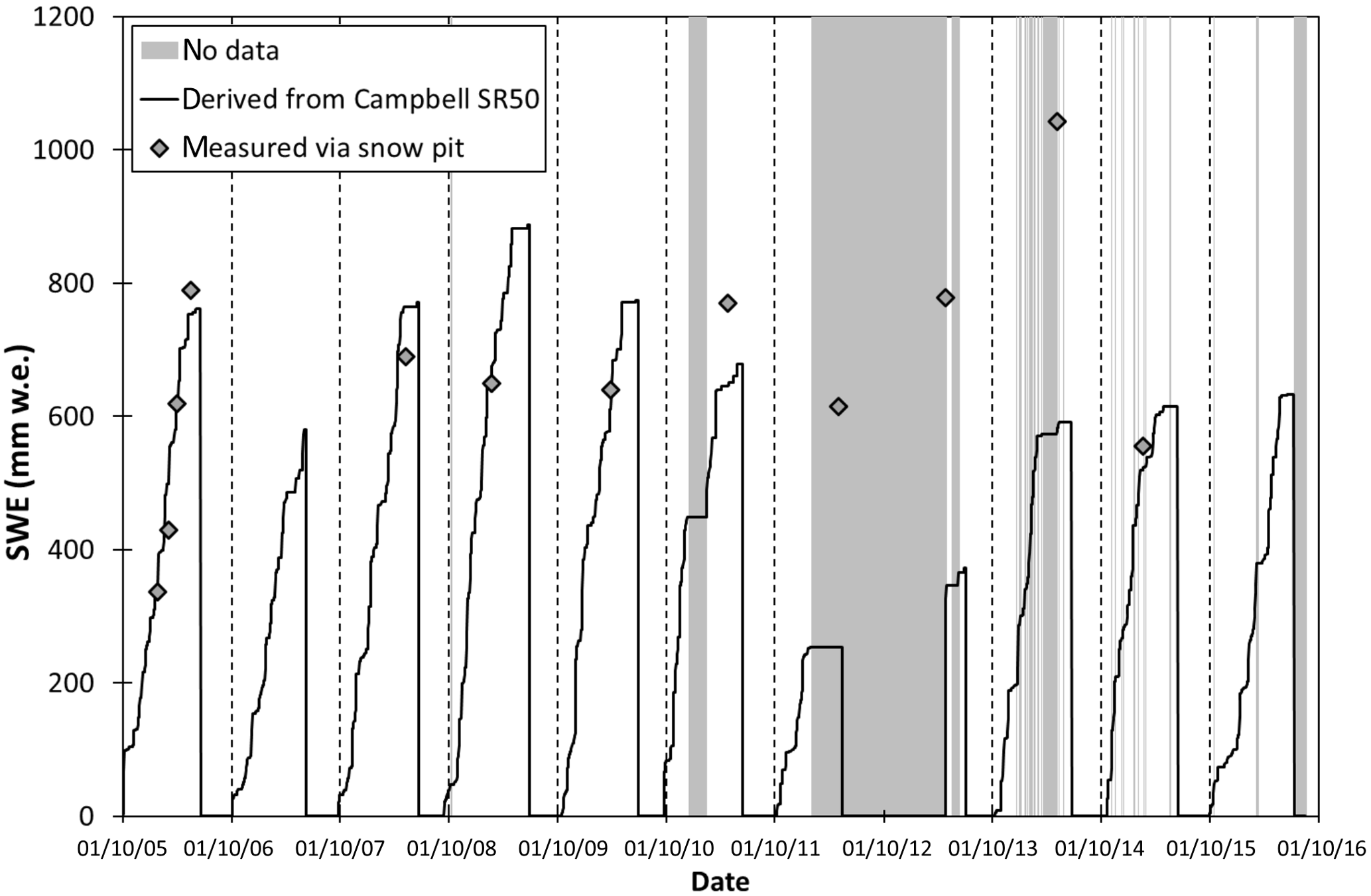
Figure 3Daily SWE data derived from snow depth by the Campbell SR50 (using the new snow density of 149 kg m−3) and measured by snow pits from 1 October 2005 to 30 September 2016. The periods without data are shown in light grey. The dates shown are dd/mm/yy.
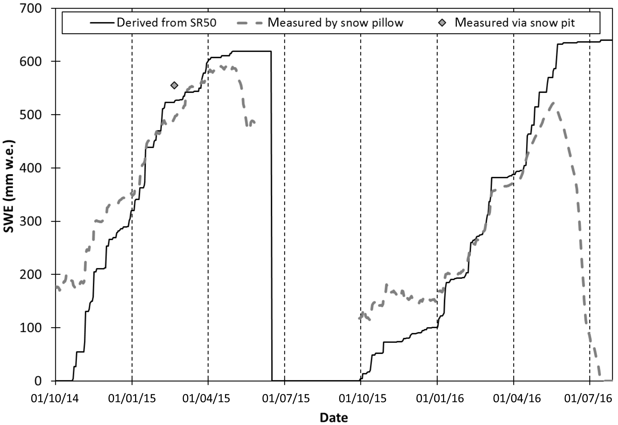
Figure 4Daily SWE data derived from snow depth measured by Campbell SR50 (using the new snow density of 149 kg m−3) and measured by snow pits and snow pillow from October 2014 to July 2016. The dates shown are dd/mm/yy.
Figure 2 represents the 11-year dataset of snow depth measured by the SR50 sonic ranger from 2005 to 2016. The last data (after October 2015) were recorded in a different site than the previous one because of the AWSs' relocation in November 2015. The distance between the two sites is about 500 m, the difference in elevation is only 44 m and the aspect is very similar, so we do not expect the site change to have a noticeable impact on the snow depth data.
Large interannual variability is seen, with a peak of 280 cm (on 2 May 2008). In general, the maximum snow depth exceeds 200 cm, except in the period 2006–2007, which is characterized by the lowest maximum value (134 cm on 26 March 2007). These values are in agreement with findings over the Italian Alps in the period 1960–2009. In fact, Valt and Cianfarra (2010) reported a mean snow depth of 233 cm (from 199 to 280 cm) for the stations above 1500 m a.s.l. The snow accumulation period generally starts in late September to early October. The snow appears to be completely melted between the second half of June and the beginning of July (Fig. 2).
Because of the incomplete dataset from the Sommer USH8 sonic ranger, only the data from the Campbell SR50 sensor are considered for analysis.
The updated value of ρnew snow is 149 kg m−3, which is similar to findings considering the 2005–2009 dataset (equal to 140 kg m−3, Senese et al., 2012a). Figure 3 reports the cumulative SWESR values (i.e., applying Eq. 4) and the ones obtained using snow pit techniques (SWEsnow-pit) from 2005 to 2016. As found in previous studies (Senese et al., 2012a, 2014), there is a rather good agreement (RMSE = 58 mm w.e. with a mean SWEsnow-pit value of 609 mm w.e.) between the two datasets (i.e., measured SWEsnow-pit and derived SWESR). Whenever sonic ranger data are not available for a long period, the derived total SWE value appears to be incorrect. In particular, in addition to the length of the missing dataset, the period of the year with missing data influences the magnitude of the underestimation of the actual accumulation. During the snow accumulation period 2010–2011, the data gap from 15 December 2010 to 12 February 2011 (a total of 60 days) produces an underestimation of 124 mm w.e. corresponding to 16 % of the measured value (on 25 April 2011 SWESR=646 mm w.e. and SWEsnow-pit=770 mm w.e.; Fig. 3). During the hydrological years 2011–2012 and 2012–2013, there were some problems with sonic ranger data acquisition thus making it impossible to accumulate these data from 31 January 2012 to 25 April 2013. In these cases, there are noticeable differences between the two datasets: on 1 May 2012 SWEsnow-pit=615 mm w.e. and SWESR=254 mm w.e., and on 25 April 2013 SWEsnow-pit=778 mm w.e. and SWESR=327 mm w.e., with an underestimation of 59 and 58 %, respectively (Fig. 3).
Figure 4 reports the comparison between the SWESR values and the ones obtained using the snow pillow (for the period 2014–2016). Apart from a first interval without snow cover, or with just a very thin layer, the SWESR curve follows that of SWE measured by the snow pillow (Fig. 4), thus suggesting that our approach seems to offer reasonable results. In order to better assess the reliability of our derived SWESR values, a scatter plot of measured SWE data (by means of snow pillow, snow weighing tube, and snow pit) versus derived is shown (Fig. 5). The period chosen is the snow accumulation time frame during 2014–2015 and 2015–2016: from November 2014 to March 2015 and from February 2016 to May 2016 (i.e., the snow accumulation period, excluding the initial period in which the snow pillow seems to have significant measuring problems). There is a general underestimation of SWESR compared to the snow pillow values, considering the 2014–2015 data, though the agreement strengthens in the 2015–2016 dataset (Fig. 5): 54 and 29 mm w.e. of RMSE regarding 2014–2015 and 2015–2016, respectively. Considering the whole dataset, the RMSE is 45 mm w.e., which proves to be about 8 % of the total SWE yearly average, as measured by the snow pillow. If compared with the snow pit, the difference is 35 mm w.e. (about 6 % of the measured value). Nevertheless, numerous measurements made using the snow weighing tube (Enel-Valtecne) around the AWSs on 20 February 2015 showed wide variations of snow depth over the area (mean value of 165 cm and standard deviation of 29 cm), even if the snow surface seemed to be homogenous. This was mainly due to the roughness of the glacier ice surface. Indeed, on the same date, the snow pillow recorded a SWE value of 493 mm w.e., while from the snow pit the SWE was equal to 555 mm w.e., and from the snow weighing tube the SWE ranged from 410 to 552 mm w.e. (Fig. 5), even if all measurements were performed very close to one another in time and space.
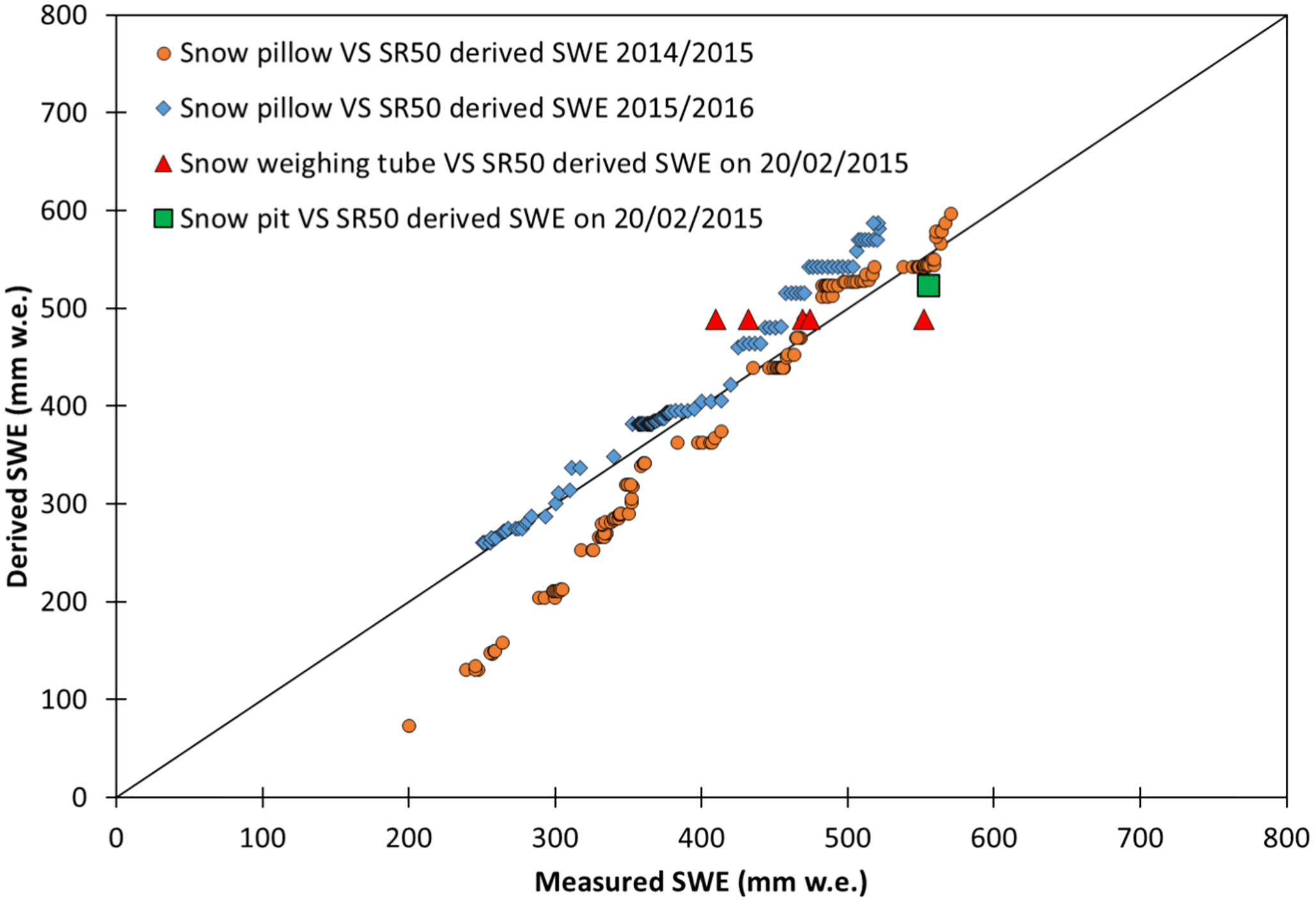
Figure 5Scatter plots showing SWE measured by snow pillow and snow pit, derived by applying Eq. (4) to data acquired by Campbell SR50 (using the new snow density of 149 kg m−3). Two accumulation periods of measurements are shown from November 2014 to March 2015 and from February 2016 to May 2016. Every dot represents a daily value.
5.1 Possible errors related to the methodology
Defining a correct algorithm for modeling SWE data is very important for evaluating the water resources deriving from snowmelt. The approach applied for deriving SWESR is highly sensitive to the value used for the new snow density, which can vary substantially depending on both atmospheric and surface conditions. In this way, the error in individual snowfall events could be significant. Moreover, the technique depends on determining snowfall events, which are estimated from changes in snow depth, and the subsequent calculation and accumulation of SWESR from those events. Therefore, missed events due to gaps in snow depth data could invalidate the calculation of peak SWESR. For these reasons, we focused our analyses on understanding how an incorrect assessment of ρnew snow or a gap in snow depth data may affect the SWE estimation.
Table 2The leave-one-out cross-validation (LOOCV). For each survey, we reported the SWE values measured by means of the snow pit (SWEsnow-pit), the values of the new snow density applying the Eq. (3) (ρnew snow from snow pit j), and the new snow density obtained applying the LOOCV method (LOOCVρnew snow).
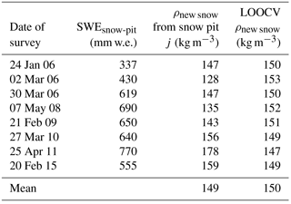
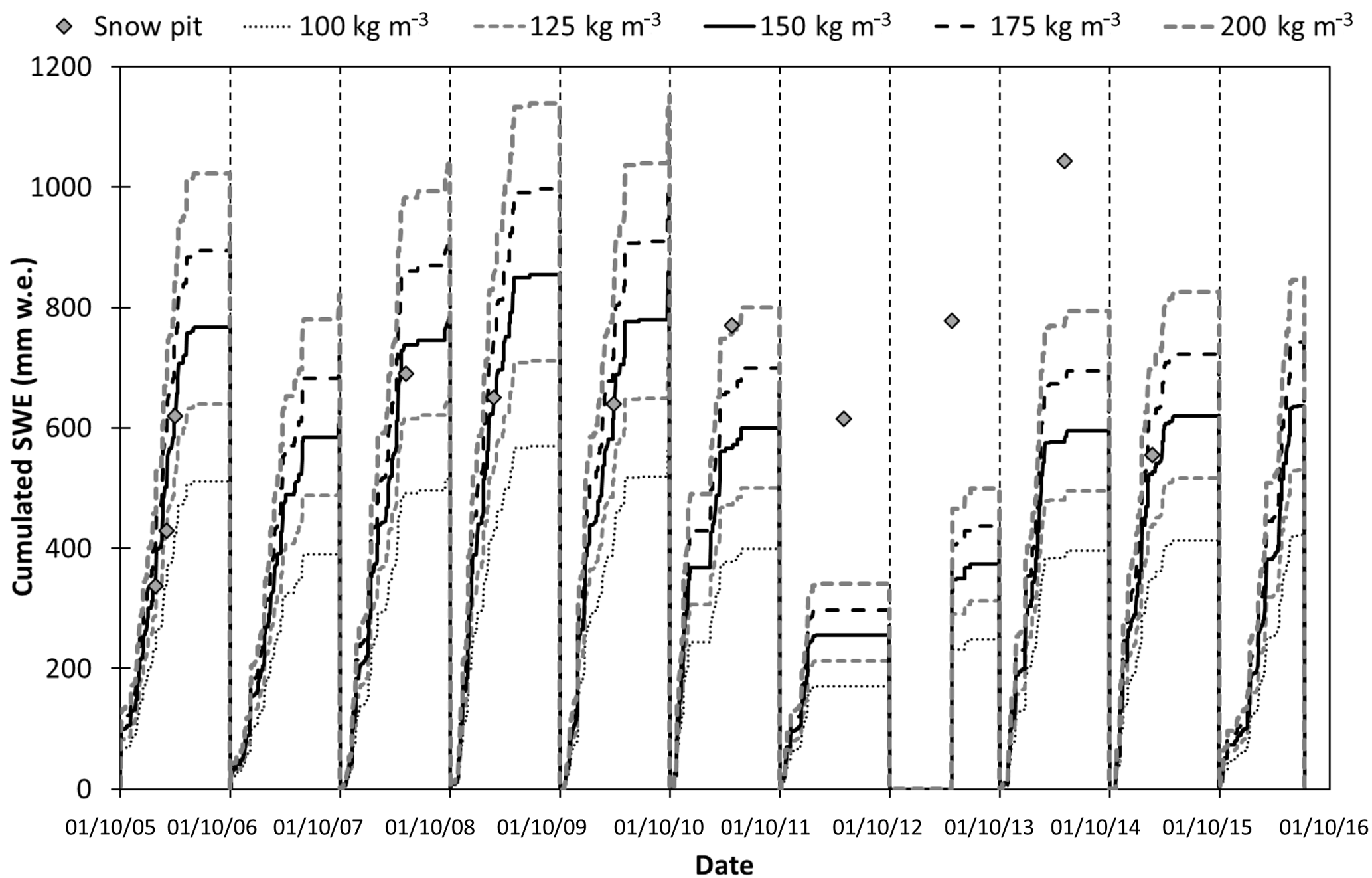
Figure 6Comparison among daily SWE values derived from snow depth data acquired by SR50 sonic ranger (applying different values of new snow density) and SWE values measured by snow pits from 2005 to 2016. The dates shown are dd/mm/yy.
First, we evaluated the ρnew snow estimate (applying Eq. 3, equal to 149 kg m−3 considering the 2005–2015 dataset), by means of the leave-one-out cross-validation technique (LOOCV, a particular case of leave-p-out cross-validation with p=1), to ensure independence between the data we use to estimate ρnew snow and the data we use to assess the corresponding estimation error. In this kind of cross-validation, the number of “folds” (repetitions of the cross-validation process) equals the number of observations in the dataset. Specifically, we applied Eq. (3) once for each snow pit (j), using all the other snow pits in the calculation (LOOCV ρnew snow) and using the selected snow pit as a single-item test (ρnew snow from snow pit j). In this way, we avoid dependence between the calibration and validation datasets in assessing the new snow density. The results are shown in Table 2. Analysis shows that the standard deviation of the differences between the LOOCV ρnew snow values and the corresponding single-item test values (ρnew snow from snow pit j) is 18 kg m−3. The error of the average value of ρnew snow can therefore be estimated dividing this standard deviation by the square root of the number of the considered snow pits. It turns out to be 6 kg m−3. The new and the old estimates (149 and 140 kg m−3, respectively) therefore do not have a statistically significant difference. The individual snow accumulation periods instead have naturally a higher error and the single snow pit estimates for ρnew snow range from 128 to 178 kg m−3. In addition, we attempted to extend this analysis considering each single snow layer (hij) instead of each snow pit j. In particular, we tried to associate the corresponding new snow measured by the sonic ranger with each snow pit layer (Citterio et al., 2007). However, this approach turned out to be too subjective to contribute accurate information about the ρnew snow value we found.
Moreover, we investigated the SWE sensitivity to changes in ρnew snow. In particular, we calculated SWESR using different values of new snow density ranging from 100 to 200 kg m−3 at 25 kg m−3 intervals (Fig. 6). An increase/decrease of the density by 25 kg m−3 causes a mean variation in SWESR of ±106 mm w.e. for each hydrological year (corresponding to about 17 % of the mean total cumulative SWE considering all hydrological years), ranging from ±43 to ±144 mm w.e. A reliable estimation of ρnew snow is therefore a key issue.
In addition to an accurate definition of new snow density, an uninterrupted dataset of snow depth is also necessary in order to derive correct SWESR values. This can also be deducted observing the large deviations between the SWE values (independent of the chosen snow density) found by the SR50 and the snow pit measurements in the years 2010, 2011, 2012, and 2013. It is therefore necessary to put in place all the available information to reduce the occurrence of data gaps to a minimum. The introduction of the second sonic ranger (Sommer USH8) at the end of the 2013–2014 snow season was an attempt to limit the impact of this problem. This second sonic ranger, however, was still in the process of testing in the final years of the period investigated in this paper. We are confident that in the years to come it can help reduce the problem of missing data. Indeed, daily variations in snow depth measured by one sensor could be used to fill a data gap from the other one. Multiple sensors for fail-safe data collection are indeed highly recommended. In addition, the four wooden stakes installed at the corners of the snow pillow at the beginning of the 2014–2015 snow season were another idea for collecting more data. Unfortunately, they were broken almost immediately after the beginning of the snow accumulation period. They can offer another way to deal with the problem of missing data, provided we figure out how to avoid breakage during the winter season. Probably the choice of a more robust and white material (such as insulated white steel) could overcome this issue.
It is also important to stress that potential errors in individual snowfall events could affect peak SWESR estimation. A large snowfall event with a considerable deviation from the mean new snow density will result in significant errors (e.g., a heavy wet snowfall). These events are rather rare at the Forni site: only 3 days in the 11-year period covered by the data recorded more than 40 cm of new snow (the number of days decreases to 1 if the threshold increases to 50 cm). Therefore, even if the proposed technique is susceptible to these errors, high precipitation amounts are infrequent, reducing the likelihood of this happening at the Forni site. Without knowing the true density of the new snow during these big events, it is difficult to understand its impact on the SWE estimate. However, assuming that the new snow density increases from 149 to 200 kg m−3, the difference in SWE for a large event (e.g., 30 cm) would be 15 mm w.e. (45 mm w.e. with 149 kg m−3 and 60 mm w.e. with 200 kg m−3).
Our new snow data could be affected by settling, sublimation, snow transported by wind, and rainfall. As far as settling is concerned, Δhsnow-pit-j from Eq. (2) would indeed be higher if Δhtj values were calculated considering an interval shorter than 24 h. However, this would not be possible because on the one hand, the sonic ranger data's margin of error is too high to consider hourly resolution, and on the other hand, new snow is defined as by the WMO within the context of a 24 h period. Settling processes can also concern the snow pack under the new snow layer. This process can affect our daily differences especially when the snowfall lasts for several days. In this case, the measured daily positive snow depth differences could be less than the real depth of the new snow, with the consequence of overestimating new snow density. However, the obtained mean new snow density is not much higher than the general values found in the literature. In addition, comparison with the snow pillow dataset seems to support our methodology. On the other hand, if many days pass between one snowfall and the following one, the settlement of the snow pack under the new snow layer is less likely to affect the measured differences in snow depth and this seems to be the case of the Forni Glacier site, since snow days account for only 9 % of the snow season days. Regarding the transport by wind, the effect that is potentially most relevant is new snow that is recorded by the sonic ranger but then blows away in the following days. It is therefore considered in Δhsnow-pit-j but not in SWEsnow-pit-j, thus causing an underestimation of ρnew snow (see Eq. 3). The snow transported to the measuring site can also influence ρnew snow, even if in this case the effect is less important, as it is measured both by the sonic ranger and by the snow pit. Here, the problem may be an overestimation of ρnew snow as snow transported by wind usually has a higher density than new snow. We considered the problem of the effect of wind on snow cover when we selected the station site on the glacier. Even though sites not affected by wind transport simply do not exist, we are confident that the site we selected has a position that can reasonably minimize this issue. Moreover, sublimation processes would have an effect similar to those produced by new snow that is recorded by the sonic ranger but then blown away in the following days. In any case, the value we found for the site average new snow density (i.e., 149 kg m−3) does not seem to suggest an underestimated value.
Finally, another possible source of error in estimating new snow density and in deriving the daily SWE is represented by rainfall events. In fact, one of the effects is an enhanced snowmelt and then a decrease in snow depth, as rainwater has a higher temperature than the snow. Therefore, especially at the beginning of the snow accumulation season, we could detect snowfall (analyzing snow depth data) but whenever it was followed by rainfall, the new fallen snow could partially or completely melt, thus remaining undetected when measured at the end of the accumulation season using snow pit techniques. This is another potential error that, besides the ones previously considered, could lead to underestimation of the ρnew snow value, even if, as already mentioned, the value of 149 kg m−3 does not seem to suggest this. On the other hand, rain can also increase the SWE measured using snow pit techniques without giving a corresponding signal in the sonic ranger measurements of snow depth whenever limited amounts of rain fall over cold snow. In any case, rain events are extremely rare during the snow accumulation period, so the errors associated with rain are minimal.
5.2 Possible errors related to the instrumentation
With regard to the instrumentation, we found some issues related to the derived snow data. Focusing on the beginning of the snow accumulation period, it appears that neither system of measurement (i.e., sonic ranger and snow pillow) was able to detect the first snowfall events correctly. With the sonic ranger, the surface roughness of the glacier ice makes it impossible to distinguish a few centimeters of freshly fallen snow. In fact, the surface heterogeneity (i.e., bare ice, ponds of different size and depth, presence of dust, and fine or coarse debris that can be scattered over the surface or aggregated) translates into a differential ablation, due to different values of albedo and heat transfer. These conditions cause differences in surface elevation of up to 10s of centimeters and affect the angular distribution of reflected ultrasound. At 3 m of height, the diameter of the measuring field is 1.17 m for the SR50. For these reasons, the sonic ranger generally records inconsistent distances between ice surface and sensor, generally much smaller than the values of the previous and subsequent readings. This issue does not occur with thick snow cover, as the snow roughness is much less than that of ice.
Regarding the snow pillow methodology, analyzing the 2014–2015 and 2015–2016 data, it seems to work correctly only with a snow cover thicker than 50 cm (Fig. 4). In fact, with null or very low snow depth, SWE values are incorrectly recorded. The results from the snow pillow are difficult to explain as this sensor has been in use for only two winter seasons and we are still in the process of testing it. Analyzing data from the years to come will strengthen our interpretation. However, we have searched for a possible explanation of this problem and the error could be due to the configuration of the snow pillow. Moreover, some of the under-measurement or over-measurement errors can commonly be attributed to differences in the amount of snow settlement over the snow pillow, compared with that over the surrounding ground, or to bridging over the snow pillow with cold conditions during development of the snow cover (Beaumont, 1965). In addition, another major source of SWE snow pillow errors is generally due to measuring problems of this device, which is sensitive to the thermal conditions of the sensor, the ground, and the snow (Johnson et al., 2015). In fact, according to Johnson and Schaefer (2002) and Johnson (2004) snow pillow under-measurement and over-measurement errors can be related to the amount of heat conduction from the ground into the overlying snow cover, the temperature at the ground/snow interface, and the insulating effect of the overlying snow. This particular situation can not be recognized at the Forni Glacier, as the surface consists of ice and not of soil. Therefore, in our particular case the initial error could be due to the configuration of the snow pillow.
In order to assess the correct outset of the snow accumulation period and overcome the instrument issues, albedo represents a useful tool, as freshly fallen snow and ice are characterized by very different values (e.g., Azzoni et al., 2016). In fact, whenever a snowfall event occurs, albedo immediately rises from about 0.2 to 0.9 (typical values of ice and freshly fallen snow, respectively; Senese et al., 2012a). This is also confirmed by the automated camera's hourly pictures. During the hydrological year 2014–2015, the first snowfall was detected on 22 October 2014 by analyzing albedo data, and it is verified by pictures taken by the automated camera. Before this date, the sonic ranger did not record a null snow depth, mainly due to the ice roughness; therefore, we had to correct the dataset accordingly.
Concerning the SWE as determined by the snow weighing tube, this device is pushed vertically into the snow to fill the tube. The tube is then withdrawn from the snow and weighed. Knowing the length of tube filled with snow, the cross-sectional area of the tube and the weight of the snow allows a determination of both the SWE and the snow density (Johnson et al., 2015). The measurements carried out around the AWSs on 20 February 2015 showed a great spatial variability in SWE (Fig. 5): the standard deviation is 54 mm w.e., corresponding to 12 % of the mean value from snow weighing tube measurements. This could explain the differences found analyzing data acquired using the snow pillow techniques, measured by the snow pit, and derived by the sonic ranger. However, the SWE variability highlighted by the snow weighing tube surveys can be also due to oversampling by this device (Work et al., 1965). Numerous studies have been conducted to verify snow tube accuracy in determining SWE. The most recent studies by Sturm et al. (2010) and Dixon and Boon (2012) found that snow tubes could under- or over-measure SWE from −9 to +11 %. Even if we allow for ±10 % margin of error in our snow tube measurements, the high SWE variability is confirmed.
Finally, the last approach for measuring SWE is represented by the snow pit. This method (like the snow tube) has the downside that it is labor intensive and it requires expert personnel. Moreover, as discussed in Senese et al. (2014), it is very important to select a correct date to take the snow pit surveys in order to assess the total snow accumulation amount. Generally, 1 April is the date considered most indicative of the peak cumulative SWE in high mountain environments of the midlatitudes, but this day is not always the best one. In fact, Senese et al. (2014) found that using a fixed date for measuring the peak cumulative SWE is not the most suitable solution. In particular, they suggest that the correct temperature threshold can help to determine the most appropriate time window of analysis, indicating the starting time of snow melting processes and then the end of the accumulation period. From the Forni Glacier, the application of the +0.5 ∘C daily temperature threshold allows for a consistent quantification of snow ablation while, instead, for detecting the beginning of the snow melting processes, a suitable threshold has proven to be at highest −4.6 ∘C. A possible solution to this problem could be to repeat the snow pit surveys over the same period to verify the variability of microscale conditions. This can be useful especially in those remote areas where no snowfall information is available. However, this approach involves too much time and resources and is not always feasible.
Even if the generally used sensors (such as the heated tipping bucket rain gauge, the heated weighing gauge, or the disdrometer) provide more accurate measurements, in remote areas like a glacier, it is very difficult to install and maintain them. One of the limitations concerns the power to be supplied to instruments, which can only consist of solar panels and lead–gel batteries. In fact, at the Forni site we had to choose only unheated low-power sensors. The snow pillow turned out to be logistically unsuitable, as it required frequent maintenance. Especially with bare ice or few centimeters of snow cover, the differential ablation causes instability of the snow pillow, mainly due to its size. Therefore, the first test of this sensor seems to indicate that it did not turn out to be appropriate for a glacier surface. We will, however, try to get better results from it in the coming years. The snow pit can represent a useful approach but it requires expert personnel for carrying out the measurements, and the usefulness of the data thus obtained depends on the date of excavating the snow pits. The automated camera provided hourly photos, but for assessing a correct snow depth at least two graduated rods have to be installed close to the automated camera. However, over a glacier surface, glacier dynamics and snow flux can compromise the stability of the rods: in fact, at the AWS Forni SPICE we found them broken after a short while. Finally, the SR50 sonic ranger features the unique problem of the definition of the start of the accumulation period, but this can be overcome using albedo data.
For the SPICE project, snow measurements at the Forni Glacier (Italian Alps) have been implemented by means of several automatic and manual approaches since 2014. This has allowed accurate comparison and evaluation of the pros and cons of using the snow pillow, sonic ranger, snow pit, and snow weighing tube, and of estimating SWE from snow depth data. We found that the mean new snow density changes based on the considered period was 140 kg m−3 in 2005–2009 (Senese et al., 2014) and 149 kg m−3 in 2005–2015. The difference is, however, not statistically significant. We first evaluated the new snow density estimation by means of LOOCV and we found an error of 6 kg m−3. Then, we benchmarked the derived SWESR data against the information from the snow pillow (data which were not used as input in our density estimation), finding an RMSE of 45 mm w.e. (corresponding to 8 % of the maximum SWE measured by means of the snow pillow). These analyses permitted a correct definition of the reliability of our method in deriving SWE from snow depth data. Moreover, in order to define the effects and impacts of an incorrect ρnew snow value in the derived SWE amount, we found that a change in density of ±25 kg m−3 causes a mean variation of 17 % of the mean total cumulative SWE, considering all hydrological years. Finally, once ρnew snow is known, the sonic ranger can be considered a suitable device on a glacier, or in a remote area in general, for recording snowfall events and for measuring snow depth values in order to derive SWE values. In fact, the methodology we have presented here can be interesting for other sites as it allows estimating total SWE using a relatively inexpensive, low-power, low-maintenance, and reliable instrument such as the sonic ranger, and it is a good solution for estimating SWE at remote locations such as glacier or high alpine regions. In addition, our methodology ensured that the mean new snowfall density can be reliably estimated.
Although conventional precipitation sensors, such as the heated tipping bucket rain gauges, heated weighing gauges, or disdrometers, can perhaps provide more accurate estimates of precipitation and SWE than the ones installed at the Forni Glacier, they are less than ideal for use in high alpine and glacier sites. The problem is that it is very difficult to install and maintain them in remote areas like a glacier at a high alpine site. The main constrictions concern (i) the power supply to the instruments, which consists of solar panels and lead–gel batteries and (ii) the glacier dynamics, snow flux, and differential snow/ice ablation that can compromise the stability of the instrument structure. Therefore, a sonic ranger could represent a useful approach for estimating SWE, since it does not require expert personnel, nor does it depend on the date of the survey (as do such manual techniques as snow pits and snow weighing tubes); it is not subject to glacier dynamics, snow flux, or differential ablation (as are graduated rods installed close to an automated camera and snow pillows), and it does not required a lot of power (unlike heated tipping bucket rain gauges). The average new snow density must, however, be known either by means of snow pit measurements or by the availability of information from similar sites in the same geographic area.
The two automatic weather stations were managed by the authors and all data were acquired by the authors. Data can be requested by email from the authors at antonella.senese@unimi.it or guglielmina.diolaiuti@unimi.it.
The authors declare that they have no conflict of interest.
This article is part of the special issue “The World Meteorological Organization Solid Precipitation InterComparison Experiment (WMO-SPICE) and its applications (AMT/ESSD/HESS/TC inter-journal SI)”. It is not associated with a conference.
The AWS1 Forni was developed under the umbrella of the SHAR (Stations at High Altitude for Research on the Environment) program, managed by the Ev-K2-CNR Association from 2002 to 2014; it was part of the former CEOP network (Coordinated Energy and Water Cycle Observation Project) promoted by the WCRP (World Climate Research Programme) within the framework of the online GEWEX project (Global Energy and Water Cycle Experiment). The AWS1 Forni and AWS Forni SPICE were included in the SPICE (Solid Precipitation Intercomparison Experiment) project managed and promoted by the WMO (World Meteorological Organization), and in the CryoNet project (core network of Global CryosphereWatch promoted by the WMO). Finally, the AWSs were applied in the ESSEM COST Action ES1404 (a European network for a harmonized monitoring of snow for the benefit of climate change scenarios, hydrology, and numerical weather prediction).
This research has been carried out under the umbrella of a research project funded by Sanpellegrino Levissima S.p.A., and the young researchers involved in the study were supported by the DARA (Department of Regional Affairs and Autonomies) of the Presidency of the Council of Ministers of the Italian Government through the GlacioVAR project (PI Guglielmina Diolaiuti). Moreover, Stelvio National Park – ERSAF kindly supported data analyses and hosts the AWS1 Forni and the AWS Forni SPICE at the surface of the Forni Glacier, thus making possible the launch of glacier micro-meteorology in Italy.
The authors acknowledge the special issue editor, Mareile Wolff, for her
help in improving the first draft of this paper and the two reviewers for
their useful comments and suggestions. The authors are also grateful to Carol
Rathman for checking and improving the English language of the
manuscript.
Edited by: Mareile
Wolff
Reviewed by: two anonymous referees
Anderson, E. A. and Crawford, N. H.: The synthesis of continuous snowmelt hydrographs on digital computer, Tech. Rep. no. 36, Department Of Civil Engineering of the Stanford University, 1964.
Azzoni, R. S., Senese, A., Zerboni, A., Maugeri, M., Smiraglia, C., and Diolaiuti, G. A.: Estimating ice albedo from fine debris cover quantified by a semi-automatic method: the case study of Forni Glacier, Italian Alps, The Cryosphere, 10, 665–679, https://doi.org/10.5194/tc-10-665-2016, 2016.
Azzoni, R. S., Fugazza, D., Zennaro, M., Zucali, M., D'Agata, C., Maragno, M., Smiraglia, C., and Diolaiuti, G. A.: Recent structural evolution of Forni Glacier tongue (Ortles-Cevedale Group, Central Italian Alps), J. Maps, 13, 870–878, 2017.
Beaumont, R. T.: Mt. Hood pressure pillow snow gauge, J. Appl. Meteorol., 4, 626–631, 1965.
Bocchiola, D. and Rosso, R.: The distribution of daily snow water equivalent in the central Italian Alps, Adv. Water Resour., 30, 135–147, 2007.
Brandes, E. A., Ikeda, K., Zhang, G., Schonhuber, M., and Rasmussen, R. M.: A statistical and physical description of hydrometeor distributions in Colorado snowstorms using a video disdrometer, J. Appl. Meteor. Climatol., 46, 634–650, 2007.
Citterio, M., Diolaiuti, G., Smiraglia, C., Verza, G., and Meraldi, E.: Initial results from the automatic weather station (AWS) on the ablation tongue of Forni Glacier (Upper Valtellina, Italy), Geogr. Fis. Din. Quat., 30, 141–151, 2007.
Currie, B. W.: Water content of snow in cold climates, B. Am. Meteorol. Soc., 28, 150–151, 1947.
D'Agata, C., Bocchiola, D., Maragno, D., Smiraglia, C., and Diolaiuti, G. A.: Glacier shrinkage driven by climate change in The Ortles-Cevedale group (Stelvio National Park, Lombardy, Italian Alps) during half a century (1954–2007), Theoretical Applied Climatology, April 2014, 116, 169–190, https://doi.org/10.1007/s00704-013-0938-5, 2014.
Diolaiuti, G. and Smiraglia, C.: Changing glaciers in a changing climate: how vanishing geomorphosites have been drivingdeep changes in mountain landscapes and environments, Geomorphologie, 2, 131–152, 2010.
Dixon, D. and Boon, S.: Comparison of the SnowHydro snow sampler with existing snow tube designs, Hydrol. Proc., 26, 2555–2562, 2012.
Fabry, F. and Szyrmer, W.: Modeling of the melting layer, Part II: Electromagnetic, J. Atmos. Sci., 56, 3593–3600, 1999.
Ferguson, S. A., Moore, M. B., Marriott, R. T., and Speers-Hayes, P.: Avalanche weather forecasting at the northwest avalanche center, Seattle, WA, J. Glaciol., 36, 57–66, 1990.
Fierz, C. R. L. A., Armstrong, R. L., Durand, Y., Etchevers, P., Greene, E., McClung, D. M., and Sokratov, S. A.: The international classification for seasonal snow on the ground, Vol. 25, Paris, UNESCO/IHP, 2009.
Fugazza, D., Scaioni, M., Corti, M., D'Agata, C., Azzoni, R. S., Cernuschi, M., Smiraglia, C., and Diolaiuti, G. A.: Combination of UAV and terrestrial photogrammetry to assess rapid glacier evolution and conditions of glacier hazards, Nat. Hazards Earth Syst. Sci. Discuss., https://doi.org/10.5194/nhess-2017-198, in review, 2017.
Gray, D. M.: Snow accumulation and distribution, in: Modeling of snow cover runoff, edited by: Colbeck, S. C. and Ray, M., Cold Regions Research and Engineering Laboratory, Hanover, NH, 3–33, 1979.
Heymsfield, A. J., Bansemer, A., Schmitt, C., Twohy, C., and Poellot, M. R.: Effective ice particle densities derived from aircraft data, J. Atmos. Sci., 61, 982–1003, 2004.
Holroyd III, E. W.: The meso- and microscale structure of Great Lakes snowstorm bands: A synthesis of ground measurements, radar data, and satellite observations, PhD dissertation, University at Albany, State University of New York, 148 pp., 1971.
Johnson, J. B.: A theory of pressure sensor performance in snow, Hydrol. Proc., 18, 53–64, 2004.
Johnson, J. B. and Schaefer, G.: The influence of thermal, hydrologic, and snow deformation mechanisms on snow water equivalent pressure sensor accuracy, Hydrol. Proc., 16, 3529–3542, 2002.
Johnson, J. B., Gelvin, A. B., Duvoy, P., Schaefer, G. L., Poole, G., and Horton, G. D.: Performance characteristics of a new electronic snow water equivalent sensor in different climates, Hydrol. Proc., 29, 1418–1433, 2015.
Judson, A. and Doesken, N.: Density of freshly fallen snow in the central Rocky Mountains, B. Am. Meteorol. Soc., 81, 1577–1587, 2000.
Key, J., Goodison, B., Schöner, W., Godøy, Ø., Ondráš, M., and Snorrason, Á.: A Global Cryosphere Watch, Arctic, 68, 48–58, doi;10.14430/arctic4476, 2015.
LaChapelle, E. R.: The density distribution of new snow, Project F, Progress Rep. 2, USDA Forest Service, Wasatch National Forest, Alta Avalanche Study Center, Salt Lake City, UT, 13 pp., 1962.
LaChapelle, E. R.: The fundamental process in conventional avalanche forecasting, J. Glaciol., 26, 75–84, 1980.
Magono, C. and Nakamura, T.: Aerodynamic studies of falling snow flakes, J. Meteorol. Soc. Jpn., 43, 139–147, 1965.
McClung, D. M. and Schaerer, P. A.: The avalanche handbook, The Mountaineers, Seattle, WA, 1993.
Muramoto, K. I., Matsuura, K., and Shiina, T.: Measuring the density of snow particles and snowfall rate, Electron. Commun. Jpn., 78, 71–79, 1995.
Nitu, R., Rasmussen, R., Baker, B., Lanzinger, E., Joe, P., Yang, D., Smith, C., Roulet, Y., Goodison, B., Liang, H., Sabatini, F., Kochendorfer, J.,Wolff, M., Hendrikx, J., Vuerich, E., Lanza, L., Aulamo, O., and Vuglinsky, V.: WMO intercomparison of instruments and methods for the measurement of solid precipitation and snow on the ground: organization of the experiment, WMO Technical Conference on meteorological and environmental instruments and methods of observations, Brussels, Belgium, 16–18, available at: https://www.wmo.int/pages/prog/www/IMOP/publications/IOM-109_TECO-2012/Session1/O1_01_Nitu_SPICE.pdf, 2012.
Pahaut, E.: Les cristaux de neige et leurs metamorphoses, Saint-Martin-d'Hères, Météo-France, Centre d'Etudes de la Neige, Monographie de la Météorologie Nationale 96, 1975.
Passarelli Jr., R. E. and Srivastava, R. C.: A new aspect of snowflake aggregation theory, J. Atmos. Sci., 36, 484–493, 1979.
Perla, R.: On contributory factors in avalanche hazard evaluation, Can. Geotech. J., 7, 414–419, 1970.
Power, B. A., Summers, P. W., and d'Avignon, J.: Snow crystal forms and riming effects as related to snowfall density and general storm conditions, J. Atmos. Sci., 21, 300–305, 1964.
Pruppacher, H. R. and Klett, J. D.: Microphysics of Clouds and Precipitation, 2nd edn., Kluwer Academic, 954 pp., 1997.
Roebber, P. J., Bruening, S. L., Schultz, D. M., and Cortinas Jr., J. V.: Improving snowfall forecasting by diagnosing snow density, Weather Forecast., 18, 264–287, 2003.
Schultz, D. M., Cortinas Jr., J. V., and Doswell III, C. A.: Comments on “An operational ingredients-based methodology for forecasting midlatitude winter season precipitation.”, Weather Forecast., 17, 160–167, 2002.
Senese, A., Diolaiuti, G., Mihalcea, C., and Smiraglia, C.: Energy and mass balance of Forni Glacier (Stelvio National Park, Italian Alps) from a 4-year meteorological data record, Arct. Antarct. Alp. Res., 44, 122–134, 2012a.
Senese, A., Diolaiuti, G., Verza, G. P., and Smiraglia, C.: Surface energy budget and melt amount for the years 2009 and 2010 at the Forni Glacier (Italian Alps, Lombardy), Geogr. Fis. Din. Quat., 35, 69–77, 2012b.
Senese, A., Maugeri, M., Vuillermoz, E., Smiraglia, C., and Diolaiuti, G.: Using daily air temperature thresholds to evaluate snow melting occurrence and amount on Alpine glaciers by T-index models: the case study of the Forni Glacier (Italy), The Cryosphere, 8, 1921–1933, https://doi.org/10.5194/tc-8-1921-2014, 2014.
Senese, A., Maugeri, M., Ferrari, S., Confortola, G., Soncini, A., Bocchiola, D., and Diolaiuti, G.: Modelling shortwave and longwave downward radiation and air temperature driving ablation at the Forni Glacier (Stelvio National Park, Italy), Geogr. Fis. Dinam. Quat., 39, 89–100, https://doi.org/10.4461/GFDQ.2016.39.9, 2016.
Smiraglia, C. and Diolaiuti, G.: Epiglacial morphology, in: Encyclopedia of Snow, Ice and Glaciers, edited by: Singh, V. P., Haritashya, U. K., and Singh, P., Sprinter, Berlin, 2011.
Sturm, M., Taras, B., Liston, G. E., Derksen, C., Jones, T., and Lea, J.: Estimating snow water equivalent using snow depth data and climate classes, J. Hydrometeorol., 11, 1380–1394, 2010.
Super, A. B. and Holroyd III, E. W.: Snow accumulation algorithm for the WSR-88D radar: Second annual report, Bureau Reclamation Tech. Rep. R-97-05, U.S. Dept. of Interior, Denver, CO, 77 pp., 1997.
Urbini, S., Zirizzotti, A., Baskaradas, J., Tabacco, I. E., Cafarella, L., Senese, A., Smiraglia, C., and Diolaiuti, G.: Airborne Radio Echo Sounding (RES) measures on Alpine Glaciers to evaluate ice thickness and bedrock geometry: preliminary results from pilot tests performed in the Ortles Cevedale Group (Italian Alps), Ann. Geophys., 60, 0226, https://doi.org/10.4401/ag-7122, 2017.
Valt, M. and Cianfarra, P.: Recent snow cover variability in the Italian Alps, Cold Reg. Sci. Technol., 64, 146–157, 2010.
Wetzel, S. W. and Martin, J. E.: An operational ingredients-based methodology for forecasting midlatitude winter season precipitation, Weather Forecast., 16, 156–167, 2001.
WMO: Solid Precipitation Measurement Intercomparison: Final report, WMO/TD-No. 872, Instruments and observing methods, World Meteorological Organization, Report No. 67, 202 pp., 1998.
WMO: Guide to Meteorological Instruments and Methods of Observation, WMO-No. 8, 7th Edn., World Meteorological Organization, 2008.
Work, R. A., Stockwell, H. J., Freeman, T. G., and Beaumont, R. T.: Accuracy of field snow surveys, U.S. Army Cold Reg. Res. and Eng. Lab., Tech. Rep. 163, Hanover, NH, 1965.