Brief communication: Sensitivity analysis of peak water to ice thickness and temperature: A case study in the Western Kunlun Mountains of the Tibetan Plateau

This study investigates the sensitivity of peak water in the Western Kunlun Mountains of the Tibetan Plateau. Using the Open Global Glacier Model (OGGM), we analyze how variations in inverted initial ice volume and temperature climate forcing under different Shared Socioeconomic Pathways (SSP) affect peak water timing and magnitude. We compare two global ice thickness datasets, revealing substantial differences in the projected peak water timing and magnitude. The results highlight that smaller initial ice volumes lead to earlier peak water occurrences, particularly under the SSP5-8.5 scenario. Temperature bias also notably influences the peak water timing by delaying its date in the region by roughly 13 years for each bias degree. These findings underscore the importance of accurate ice thickness estimates and climate projections for predicting future water availability and informing water management strategies in glacier-dependent regions.

1 Introduction

Modeling the future evolution of glaciers is essential due to their significant impact on sea level rise (0.61 ± 0.08 mm Sea Level Equivalent – SLE – yr⁻¹ for the 2006–2015 period (Hock et al., 2019), 0.75 ± 0.04 mm yr⁻¹ for 2000–2023 (GlaMBIE, 2025)) and freshwater resources. Consequently, the projected changes in runoff will impact downstream water management (Hock et al., 2019). With increasing air temperatures, glacier ablation and therefore glacier runoff is expected to rise and reach a maximum (if it is not already reached as it is the case in many regions), defined as “peak-water”, after which glacial freshwater outputs will decline due to the shrinking glacier area (Huss and Hock, 2018). Determining the precise timing and magnitude of maximum runoff is therefore of prime importance for freshwater management, likely affecting ecosystems, drinking water resources as well as other sectors such as agriculture or hydro-power production (Arias et al., 2021).

However, projections of glacier runoff remain uncertain due to biases in both climate forcing and initial glacier geometry, and especially ice thickness estimates (Huss and Hock, 2015). Inversion of ice thicknesses is a major source of uncertainty, influencing modeled ice volumes and consequently the timing of peak water (Huss and Farinotti, 2012). Recent advances in satellite remote sensing have produced new global datasets, such as ice thickness maps derived from surface flow velocities (Millan et al., 2022) and global estimates of glacier mass change (Hugonnet et al., 2021). Yet large discrepancies persist between these datasets, particularly in High Mountain Asia, where total ice volume estimates differ by up to 35 % between products (Farinotti et al., 2019a; Millan et al., 2022).

The Western Kunlun Mountains are located at the northern edge of the Tibetan Plateau. This is a major glacierized region within the Tarim Interior River Basin (TIRB), where glacial meltwater contributes to downstream water resources (Immerzeel et al., 2020). Despite its importance, this region is subject to the largest discrepancies among existing ice thickness datasets, making it an ideal case to illustrate how geometry uncertainty influences modeled glacier runoff. While several studies have investigated the estimation of peak water at regional and global scales (Huss and Hock, 2018; Caro et al., 2025), there are to date, few quantitative assessments of how uncertainties in initial glacier geometry and climate model biases influence its timing and magnitude.

In this study, we examine how uncertainties in ice thickness estimates and temperature affect the timing, magnitude, and duration of peak water in a region with strong vulnerability to climate change in terms of water supply (Immerzeel et al., 2020): the Western Kunlun Mountains on the Tibetan Plateau. We first integrate different ice thickness inversions into the OGGM model by recalibrating the creep parameter A to match the corresponding total glacier volume, with an approach that can be applied globally. We then perform sensitivity experiments by perturbing both initial ice volume and climate forcing to quantify their combined effects on peak water. Finally, we illustrate the role of glacier geometry by comparing two widely used ice thickness datasets that differ substantially in this region.

2 Data and Methods

2.1 Region of interest

Our study focuses on the northern part of the Karakoram, more precisely within the Western Kunlun mountain range, situated at the confluence of the Xinjiang Autonomous Region and the Tibetan Plateau. This study specifically targets a group of 160 glaciers with a total surface area of approximately 2900 km², calculated with the RGI v6 (RGI Consortium, 2017) (Fig. 1), which was used in the two ice thickness datasets that are being evaluated in this study. The glaciers are located at very high elevations (5500–6400 m, Ke et al., 2015) in a region characterized by largely sub-zero temperatures, often reaching −10 °C on annual averages. This region has an icefield-like geometry that is hosting a large variety of glaciers. The northern part of the selected region has a steeper terrain, with mostly valley glaciers, while the southern region has a less marked relief with glacial features close to the geometry of an ice cap (Ke et al., 2015). Surface flow velocities derived from radar measurements spanning from 2003 to 2011 reveal that nearly 70 % of the largest glaciers in the region exhibit a normal flow type, characterized by a continuous downstream flow. Additionally, 10 % of the glaciers are identified as surging glaciers, while the remaining 20 % display nearly stagnant velocity profiles (Yasuda and Furuya, 2013).

In terms of mass balance, Western Kunlun is within the region of High Mountain Asia affected by what is called the “Karakoram anomaly”: in 2000–2016, glacier mean elevation change (0.26 ± 0.07 m we yr⁻¹) and region-wide mass balance (0.14 ± 0.08 m we yr⁻¹) were mostly positive (Brun et al., 2017). However, during the 2000–2019 period (Hugonnet et al., 2021) found a regional mean elevation change rate of −0.23 ± 0.04 m yr⁻¹ for the Central Asia region (RGI region 13, RGI Consortium, 2017), where Western Kunlun is located, indicating an overall downward trend. Specifically, their findings highlight a shift towards thinning particularly notable in the late 2010s, signifying a potential conclusion to the previously observed Karakoram anomaly.

Furthermore, the glaciers within the scope of this study are situated in the TIRB as indicated by the green shading in Fig. 1a (Lehner et al., 2008). Specifically, the Kunlun mountain range serves as a primary water source for the Tarim River, a key component of the TIRB, which flows across the Tarim desert (Gao et al., 2010). According to Immerzeel et al. (2020), the water tower unit of Tarim Interior is defined as the overlap between the Tarim Interior hydrological basin from Lehner et al. (2008) and various mountain ranges from Körner et al. (2017) within the basin. This unit plays a pivotal role in providing water to ecosystems and the downstream population. Tarim is recognized by Immerzeel et al. (2020) as one of the most significant water units in Asia, with a notably high contribution of glacier water yield compared to precipitation in the basin. Despite this, the downstream supply often struggles to meet the increasing water demand driven by industrial, domestic, and primarily irrigation needs in the case of TIRB (Immerzeel et al., 2020). Consequently this basin stands out as one of the most vulnerable, susceptible to the impacts of climate, political, and socioeconomic changes (Immerzeel et al., 2020). A study focusing on glacier runoff changes using GloGEM (Huss and Hock, 2018) already anticipates a rise in Tarim's annual glacier runoff until around 2050, followed by a consistent decline for the remainder of the 21st century under the Representative Concentration Pathway (RCP) 4.5 emission scenario.

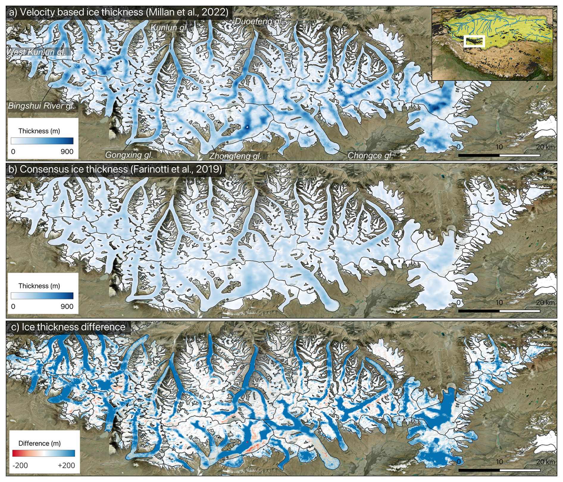
Figure 1 Map of the study region: (a) ice thickness from Millan et al. (2022) (with the location of the study set in the Himalayan area); (b) ice thickness from Farinotti et al. (2019a); and (c) difference between (a) and (b). Glacier boundaries are from the RGI v6 (RGI Consortium, 2017). Basemap is a mosaic of images from Copernicus Sentinel-2 data generated via sentinel-hub (Sinergise Solutions, 2025). Green area on the insert map corresponds to the Tarim Interior River Basin.

2.2 Ice thickness dataset

In this study, we compare the timing and magnitude of the peak water simulated using two existing global ice thickness datasets. The first is the consensus obtained in 2019 (abbreviated FARI19, Fig. 1b, Farinotti et al., 2019a), which provides a global estimate (except for the Greenland and Antarctic ice sheets) of ice volumes for individual glaciers using a combination of up to five different models selected from the Ice Thickness Inter-comparison Project (ITMIX, Farinotti et al., 2017). Inversion methods are based on the use of the principle of mass conservation (Huss and Farinotti, 2012; Maussion et al., 2019), empirical relationships between basal shear stress and glacier elevation change (Linsbauer et al., 2012), or the use of flux thickness inversion (Fürst et al., 2017). One common approach among these models (excepted for Fürst et al., 2017) is the use of flowline inversions “glacier by glacier”, based on elevation data from Digital Elevation Models (DEMs). The second ice thickness model used in this study (abbreviated MIL22, Fig. 1a, Millan et al., 2022) is based on the inversion using jointly surface ice flow velocity and surface slopes. This inversion makes use of a new global ice velocity product which provides measurements for 98 % of the world's glaciers in the years 2017–2018, at a sampling resolution of 50 m. Inversions are also based on the Shallow Ice Approximation (SIA) (Hutter, 1983), but are performed regionally and in two dimensions. This approach revealed a different picture of the distribution of ice thicknesses and the ice volume of some regions around the Earth (Millan et al., 2022; Hock et al., 2023; Frank and van Pelt, 2024), with notable differences specifically in the RGI region of this study. The Himalayan region is indeed one of the most uncertain in terms of ice thickness inversion, with very few direct field observations available to constrain the physical parameters of the inversion. In-situ measurements on fewer than 10 glaciers were available to calibrate the results of Millan et al. (2022) in the entire High Moutain Asia, and Farinotti et al. (2019a) used thickness measurements from the Glacier Thickness Database (GlaThiDa) v2 (WGMS, 2016), with less than 50 glaciers being covered within this RGI region.

In this paper, we focus on differences within a sub-region of the Western Kunlun Mountains. The consensus model corresponds approximately to the year 2000: the selected glaciers' RGI outlines are from 2010, but FARI19 used the 2000–2001 SRTM DEM for thickness inversions in this region. Since Millan et al. (2022) relies on ice velocities centered on 2017–2018, we corrected the MIL22 estimates to obtain thicknesses corresponding to the year 2000. As correction, we simply subtracted average glacier thickness changes of Hugonnet et al. (2021) between 2000 and 2019, which is obtained from DEM differencing, to MIL22 thicknesses. While solving temporal ambiguities of the thickness models is complicated, since DEM sources and in-situ data are not properly dated, this correction may be a step toward roughly matching the timing of the consensus estimate. After correction, differences in glacier mass change average about 6 km³ compared to the original MIL22 estimate, representing 1 % of the latter. Finally, the ice volume totals 345 km³ and 570 km³ for FARI19 and corrected MIL22 respectively (Fig. 1c). It is worth noting that in general, ice thickness is systematically higher for MIL22 than for Farinotti, both at low and high elevations (Fig. 1c), with differences reaching up to 200 m along glacier trunk.

2.3 Open Global Glacier Model (OGGM) – v1.6.2

OGGM is an open-source glacier evolution model that uses RGI outlines (RGI Consortium, 2017) and topographical data from various sources (NASADEM, COPDEM, GIMP, TANDEM or MAPZEN depending on the glacier location) to compute flowlines made of evenly distributed grid points, which are assigned geometrical cross-sections corrected in respect to the altitude-area distribution of the glacier (Maussion et al., 2019). Surface mass balance is calculated for each cross section according to a temperature-index model with a single temperature sensitivity factor for the entire glacier (Marzeion et al., 2012; Maussion et al., 2019). The monthly surface mass balance is calculated as the sum of accumulation and ablation on the glacier, which are a function of air temperature and precipitation. For this purpose, OGGM retrieves gridded climate data, that can be observational time series for historical runs as well as climate projections for future simulations. The surface mass balance model is calibrated on geodetic mass balance observations obtained from remote sensing (Hugonnet et al., 2021) for the 2000–2019 time period, using the W5E5v2.0 climate dataset as forcing (Lange et al., 2021). With these surface mass balance estimates as input, OGGM uses a flux-based ice flow model to solve a mass conservation equation along flowlines, under the SIA hypothesis, deriving ice thickness at each cross section. We also make use of a new feature of OGGMv1.6.2 which is a dynamic spin-up that can provide the glacier's initial state for the RGI inventory year by reconstructing its recent past while ensuring that modeled glacier area and observed one are matched within 1 % at the inventory date under historical climate forcing (Aguayo et al., 2024; Zekollari et al., 2024). Finally, the model gives as simulation outputs glacier volume, length and area, as well as glacier runoff. Considering a fixed initial glacier area including glacierized and increasingly non-glacierized terrain, the annual total runoff computed in OGGM is derived as the sum of snow melt on ice-free area, the ice and seasonal snow melt on glacier, the liquid precipitation on glacier, and the liquid precipitation on ice-free area (e.g. in Fig. S1).

2.4 Climate forcing

To compute monthly glacier surface mass balance, we use monthly temperature and precipitation time series as forcings. The W5E5 dataset (spatial resolution of 0.5°) is used by OGGM as the standard baseline climate for the period 1979–2019 during dynamical spin-up or historical runs. In order to perform projection runs extending from 2020 until 2300, we use General Circulation Models (GCM) climate data with resolution ranging 1.12–2.5° originating from the Coupled Model Intercomparison Project CMIP6 (Eyring et al., 2016), which employs Shared Socioeconomic Pathways (SSP) as scenario framework (Riahi et al., 2017). Out of the 6 different GCMs extending until 2300 available in OGGM, this study is carried out with 5 of them : MRI-ESM2-0, CESM2-WACCM, IPSL-CM6A-LR, ACCESS-CM2 , and ACCESS-ESM1-5. CanESM5 is omitted on the grounds of providing an unrealistic temperature increase in the region. The reanalysis data from 2000–2019 is used as reference climatology for bias correction of the 5 GCMs, following the anomaly method implemented in OGGM. Simulations are conducted with the “r1i1p1f1”-tagged ensemble member for each GCM under three different pathways: SSP1-2.6, SSP5-3.4-Overshoot (OS) (only 3 of the GCMs are forced under this scenario) and SSP5-8.5. It must be acknowledged that SSP5-3.4-OS is actually not an intermediate scenario since it explores the implications of a peak and decline in forcing during the 21st century (Lee et al., 2021). The choice to use a rather small number of GCMs would be inaccurate if we were trying to assess accurately and precisely the future evolution of glaciers, but here we are solely interested in the study of the impact of different ice thickness datasets on glacier evolution and their runoff.

2.5 Integration of ice thickness datasets into OGGM

Since OGGM is based on a flowline representation of glacier geometry, limitations can be found when incorporating large two dimensional datasets from remote sensing observations. Consequently, the assimilation of such thickness models into OGGM is not a trivial question. In this paper we have chosen to investigate the influence of the total ice volume on the glacier contribution to runoff, hence we do not explore spatial differences between ice thickness models. To integrate ice thickness inversions in OGGM, we first calculate from the different products the total ice volume for each glacier entity in the region of interest. Secondly, we invert ice thicknesses within the model framework (Sect. 2.3). Finally, the creep parameter A – that describes ice deformation – is calibrated in order to reach the total volume calculated with the observed datasets. If the model cannot converge on a consistent value of the creep parameter, a non-zero sliding parameter f_s is added, taking into account that it is normally set to zero for all glaciers (Maussion et al., 2019). This approach avoids model instabilities that can be found during spin-up processes, with the direct integration of ice thickness datasets in OGGM. Indeed, the latter could potentially disrupt the whole glacier dynamics, since the observed ice thicknesses might not be consistent with its modeled volume or its DEM, for example, which could lead to a numerical shock at the beginning of the simulation.

After performing the ice thickness inversions, we find a difference of 0.3 % ± 1.9 % with the volume derived from the ice thickness data calculated from Millan et al. (2022) and Farinotti et al. (2019a) (the error is the standard deviation of differences over the 160 glaciers). This is negligible compared to the difference between the two ice thickness datasets which is roughly 40 % (Millan et al., 2022; Farinotti et al., 2019a) in the study region. Once the ice thicknesses assimilation process is done, glaciers are initialized for the year 2020 by running the OGGM dynamic spin-up starting in 2000, setting up the initial conditions to be used for this study's simulations.

2.6 Peak water calculation

We assess the impact of initial ice thickness on glacier hydrological surface mass balance outputs, and more specifically on the timing and magnitude of the peak water. After performing simulations for all glaciers with different ice thicknesses, we consider the sum of all their annual runoff as the regional annual runoff, which is then averaged over a 11-year window in order to smooth inter-annual variability and highlight long-term trends. While the principle of peak water is often presented as a single maximum value (Huss and Hock, 2015), our simulations often reach a maximum regional runoff “plateau”, which can remain constant for several years or even decades. To measure the extent of this plateau, we empirically chose to define it as the top 5 % of simulated runoff values for SSP5-8.5 (and as the top 10 % for other SSPs). To pick one single date value for peak water timing, we selected the median date of the plateau's temporal extent. Similarly for the associated quantity of water runoff, we use the average of the plateau's values.

It is worth noting that, starting from glacier equilibrium and considering a climate that has warmed enough to cause substantial glacier retreat, peak water represents the tipping point beyond which any additional warming leads to a decline in glacier contribution to basin runoff (Huss and Hock, 2015). In other words, considering a moderate climate warming followed by a temperature decrease, we can reach a temporary maximum of glacier runoff that looks like an “apparent” peak water but is not a tipping point. To additionally investigate the initial ice volume influence on peak water, we design an ensemble of simulations multiplying this volume (using MIL22 initial ice thicknesses, see Sect. 2.5) by a coefficient ranging from 0.1 to 2 for all glaciers. We do not use the dynamical spin-up in this set up since it can not converge to match the RGI area with the amount of simulated reduced or increased ice volume. Instead, after ice thicknesses assimilation we simulate glaciers evolution from 2000 to 2020 simply using historical W5E5 data to initialize glaciers before future projections (see Sect. 2.4). Similarly, we examine the influence of air temperature on peak water. To this aim, we conceive an ensemble of projection runs (also using the MIL22 dataset) adding a uniform temperature bias (ranging −5 to 5 °C) over the full simulation period, meaning that this bias is added to the air temperature time series used by the model to calculate surface mass balance (additionally to any bias calculated for the mass balance calibration, see Sect. 2.3).

3 Results

3.1 Peak water sensitivity to initial volume and temperature

Our results clearly indicate that a smaller initial ice volume leads to an earlier occurrence of peak water (Fig. 2a). Glacier runoff curves for SSP1-2.5 and SSP5-8.5 follow a similar trend, with the latter being 10–20 years above the first for the same initial ice volume. Under both scenarios, multiplying this volume by a factor of two is delaying the timing of peak water by roughly 25 years (e.g., reaching after 2115 under SSP5-8.5). Similarly decreasing the initial ice volume by a factor of 0.1 will advance peak water by 25 and 20 years for SSP1-2.6 and SSP5-8.5, respectively. The magnitude of annual runoff at peak water also increases with initial ice volume but trends differ more between scenarios (Fig. 2b): for SSP1-2.6 it rises slightly from ∼ 100 to ∼ 125 m³ s⁻¹ going from a multiplying factor of 0.1 to 1.5, and then remains constant at this level for higher initial ice volumes. Regarding SSP5-8.5, runoff starts at 160 m³ s⁻¹ for a 0.1 factor and then constantly rises. Indeed, doubling the initial ice volume causes an increase of 45 % in annual runoff at peak water, reaching 380 m³ s⁻¹.

Under SSP5-8.5 temperature bias linearly influences peak water timing (Fig. 2c): being in average advanced by 12.5 years for each 1 °C increase in temperature bias. However, the magnitude of peak water does not change significantly with temperature bias, varying by roughly ±10 % compared to the magnitude without any temperature adjustment. This is not the case for the most optimistic scenario, where runoff at peak water linearly rises with positive temperature bias at a rate of 35 m³ s⁻¹ per added degree Celsius, reaching almost the same level as SSP5-8.5 with a 5 °C bias. Under SSP1-2.6, adding a lower negative bias is delaying peak water by no more than 10 years, until there is a sudden increase between −3.5 and −5 °C. Conversely, positive temperature bias almost linearly advances peak water timing, reaching the same year (i.e. 2030) as SSP5-8.5 for a 5 °C bias.

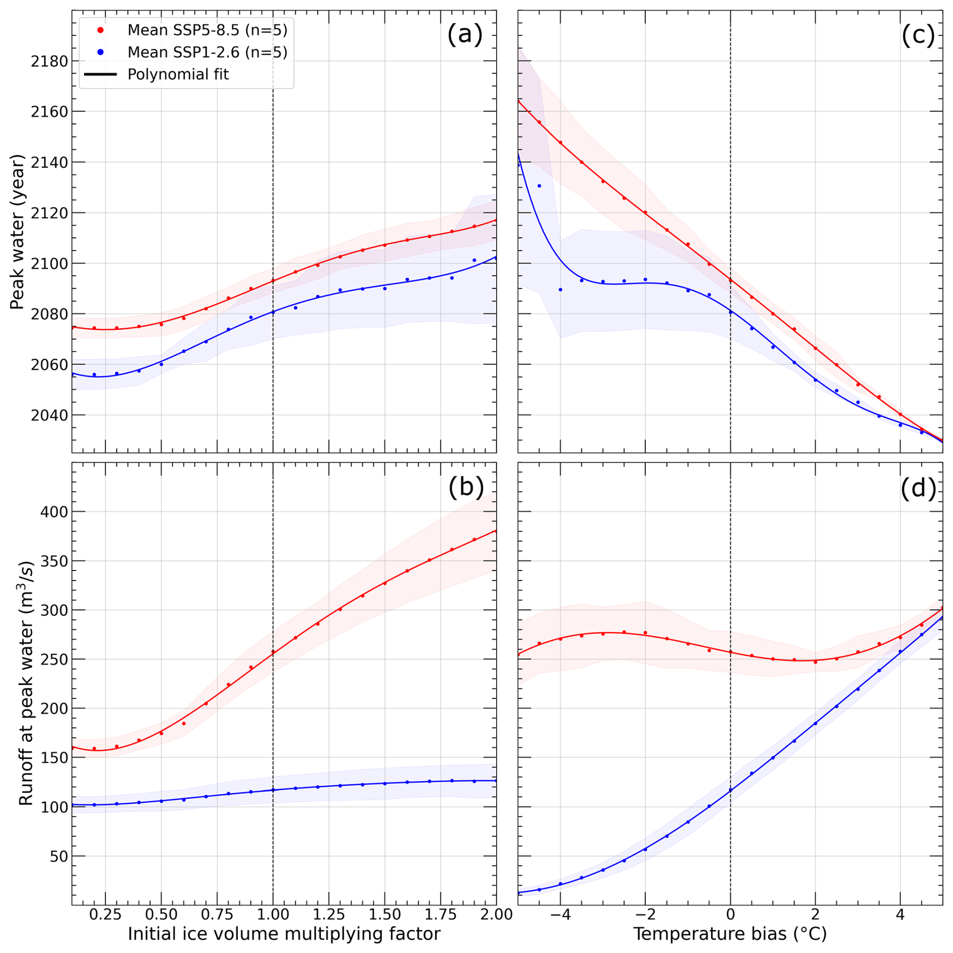
Figure 2 Timing and runoff at peak water for varying initial ice volume fractions (a–b) and temperature biases (c–d). All of these simulations have been carried out using ice thickness data from MIL22. Results are presented only for SSP-1.2.6 and SSP-5.8.5 (few differences are visible between SSP1.2.6 and SSP5.3.4-OS) with multi-GCM mean shown in bold and shading indicating the mean ±1 standard deviation of the GCM ensemble.

3.2 Future projections of evolution using existing ice thickness models

Monthly climate conditions (averaged over a 21-year window) in the region vary for the different GCMs (Fig. 3d). The standard deviation of the GCM ensemble increases along the decades after 2050, especially under SSP5-8.5, reaching approximately 4.5 °C and 0.12 mm d⁻¹ in 2300 for temperature and precipitation respectively. The forcing pathways begin to diverge notably around 2035 for mean temperature and precipitation. Regarding temperature, it slowly rises from lower than −6 °C, further continues increasing until around 2235 under the SSP5-8.5, and then stabilizes at 9 °C. Under scenario SSP1-2.6, temperature maintains constant at −4.5 °C for 2050–2100, declines until −5 °C throughout the next 50 years and remains nearly steady until 2300. Precipitation rises by almost 70 % between 2020 and 2300 for the SSP5-8.5. After an increase of less than 10 % during the 21st century, precipitation slightly declines from 2100 and then keeps roughly constant from 2150 below 0.14 mm d⁻¹ in SSP1-2.6. SSP5-3.4-OS mostly follows trends of SSP1-2.6 with a maximum deviation reaching 0.5 °C and less than 0.02 mm d⁻¹ in temperature and precipitation during the 2050–2120 period.

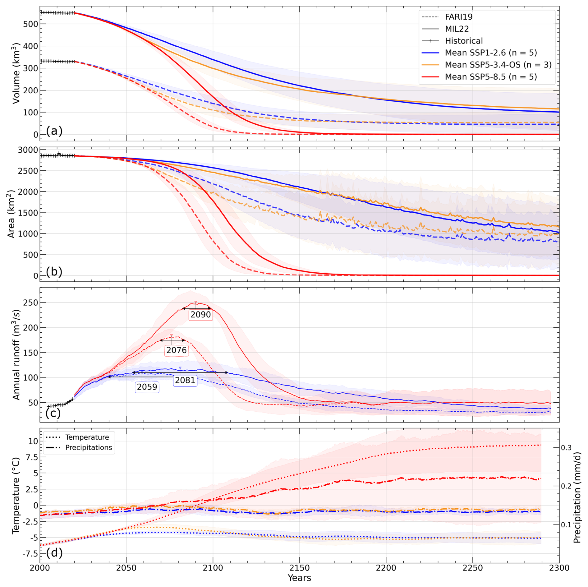
Figure 3 Projections of glacier evolution in the region of interest: the cumulative of all 160 glaciers (a) volumes, (b) areas and (c) annual runoffs, with an assessment of peak water timing, accompanied by (d) mean temperatures and precipitation projections under various SSPs (multi-GCM mean shown in bold, shading is the mean ±1 standard deviation of the GCM ensemble).

The significant differences between the two ice thickness datasets translate into an equally important one for glaciers ice volume loss (Fig. 3a). After the dynamic spin-up and before future projections simulations, regional volume calculated from FARI19 (∼ 330 km³) represents 60 % of that computed from MIL22 (∼ 550 km³) (Fig. 3a). We note that these ice volumes are lower than those computed in Sect. 2.2, both by roughly 4 %: this is a recognized weakness of OGGM's dynamical spin-up that glacier area and volume are not strictly the same at the glacier inventory date as after the inversion. Under SSP1-2.6, the total volume of ice equals ∼ 100 km³ and ∼ 25 km³ in 2300 for MIL22 and FARI19 respectively. This translates into a volume reduction of 92 % for FARI19 and 82 % for MIL22. Under SSP5-8.5, the volumes declines at a higher rate after 2040, so that very few ice volume is remaining from 2150 onwards (9 km³ and 0.7 km³ for MIL22 and FARI19 respectively). For both datasets, less than 1 km³ of ice persists at the end of the 23rd century. Trajectories under SSP5-3.4-OS follow the ones forced with SSP5-8.5 until after 2060; then volumes change trends to reach and overtake the ones of SSP1-2.6 in 2175.

As glaciers lose mass, we can also see their surface area receding. The regional glacierized surface area (∼ 2850 km² at the beginning of simulations) slowly decreases until trends start to differ between climate scenarios around 2045 (Fig. 3b). The glacierized area of the consensus decreases at a faster rate than the one of MIL22 for SSP1-2.6 with a loss of ∼ 13 km² yr⁻¹ against ∼ 7 km² yr⁻¹ in average for the 2050–2150 time period. Hence, in 2300 FARI19 and MIL22 areas have declined by 72 % and 63 % respectively. Curves based on the SSP 5-8.5 still stand out with a higher loss rate, which is very similar for FARI19 and MIL22, averaging ∼ 27 km² yr⁻¹ during 2040–2150, before most glaciers disappear completely. Indeed, while in 2150 there is still a total glacierized area equivalent to 114 and 12 km² for MIL22 and FARI19 respectively, less than 2 km² remain in 2300 for both datasets. As a brief aside, it should be noted that the visible increase in glacier area variability after 2160 reflects a known OGGM limitation, that arises from the use of a trapezoidal bed and the absence of a ice–snow distinction among others.

In response to such changes in glaciers characteristics, glacier hydrological contributions are also modified along the decades. Here, we present simulated annual runoff averaged over a 11-year window for better readability (Fig. 3c); for the same reason, we do not show simulations forced with SSP5-3.4-OS on this figure, but they are included in Fig. S2. Runoff starts at the same level for the two datasets, being around 45 m³ s⁻¹, since the initial glacier surface area is identical for all simulations. Under SSP1-2.6, after the first decades of simulation, FARI19 annual runoff goes from 45 to 105 m³ s⁻¹ in year 2059. The plateau around this “peak” lasts approximately 40 years before glaciers runoff slowly diminishes until reaching a runoff of 30 m³ s⁻¹ in 2240 and remaining constant for the last five decades of simulation. MIL22 runoff also rises from 45 to 115 m³ s⁻¹, with a peak located in year 2081 and a plateau of more than 50 years, and then declines during the following decades. In the year 2290, the runoff value is less than 40 m³ s⁻¹. Under SSP5-3.4-OS, FARI19 annual runoff reaches peak water at 125 m³ s⁻¹ in 2056, while it is assessed at 135 m³ s⁻¹ in 2061 using MIL22. In both cases, runoff declines after a plateau lasting 25–30 years depending on the dataset, before going below runoff levels of SSP1-2.6 (Fig. S2). Under SSP5-8.5, annual runoff increases steadily until reaching a peak of 180 m³ s⁻¹ in year 2076 for FARI19. For MIL22, runoff increases to a peak of almost 250 m³ s⁻¹ in 2090. In both cases, the plateau lasts 10–15 years (Fig. 3c). Then, the two annual runoff curves decline with an offset in time, and an average runoff difference of ∼ 40 %. This difference becomes smaller before fading away completely around 2190, when glaciers shrank so much that runoff is from now on almost entirely composed of snow melt and liquid precipitation on ice-free areas as indicates the evolution of annual runoff decomposed by its four different contributions (Fig. S1). The latter highlights that under SSP1-2.6 and after 2200, runoff is mostly sustained by snow melt of ice-free areas with FARI19, whereas ice melt on glacier remains the largest component with MIL22. Under SSP5-8.5 annual runoff is largely due to precipitation on ice-free areas with both datasets. Trends in runoff also highlights an abrupt change in the runoff component related to snow and ice melt on glacier around 2020 at the transition between historical and projection estimates (Figs. 3, S1), also reported in other studies (Aguayo et al., 2024). This is likely due to discrepancies in climate data between the historical and projections periods, and more specifically in the precipitations estimates (see Fig. S3). Because the mass-balance model parameters are calibrated on the historical period, substantial differences may prevent the model from being properly adjusted to future climate conditions. Glaciers runoff projections are indeed influenced by uncertainties in reference climate conditions and calibration choices (Schuster et al., 2023; Aguayo et al., 2024).

4 Discussion

4.1 Peak water dynamics and sensitivity

Our study reveals that the timing and magnitude of peak water are significantly influenced by the initial ice volume of glaciers under certain conditions. This sensitivity underscores the importance of accurate ice thickness estimations to predict future water availability (Fig. 2). Contrasting responses observed between emissions scenarios highlight the non-linear influence of climate forcing on glacier runoff. The analysis reveals a particular sensitivity of the study region to the ice thickness model under the SSP5-8.5 scenario, which presents conditions sufficient for glaciers to reach a peak water tipping point and toward an ineluctable decrease of their contribution to river runoff, unlike SSP-1.2.6 (see below). Differences in the initial ice volume also have a significant influence on the magnitude of peak water (Fig. 2). As shown in Figs. 2 and 3, a thicker glacier will at the same time provide more ice for runoff, but will also take longer to melt at lower elevations, keeping ice lower and more out of balance with the climate. This will translate into more negative surface mass balance rates, which in turn will produce increased runoff.

In the case of the SSP1-2.6 scenario, changes in the magnitude of peak water between the two datasets are not particularly significant (Figs. 2 and 3). This can be explained by the impact of the chosen climatic region for the simulations. Indeed, the projected climate under SSP1-2.6 is not warm enough to raise the equilibrium line to reach the conditions required for peak water. Thus, runoff evolution under the optimistic scenarios largely follows the temperature and precipitation trends, which in this case stabilizes after 2050 (Fig. 3d). Therefore, it is possible that in this specific case, peak water as a tipping point is never reached, and what we can see in the simulation results could more likely be identified as a melting peak, and the same applies to simulations conducted with SSP5-3.4 (Fig. S2). It is worth noting that the glacier volume and area continue to decrease during the entire time period, and that all results concern the average behavior of 160 different glaciers.

Within the temperature range explored in this study, it appears that peak water is more sensitive to temperature uncertainty than to differences in initial ice volume, in terms of peak water timing but also of peak water runoff under SSP1-2.6. The sudden increase in peak water timing under this scenario towards coldest bias is quite difficult to interpret and may be linked to the method we use to measure peak water as a plateau: the climate is so cold that actually peak water is not occurring, runoff is remaining constant at a low level, and this is largely delaying what is assessed as the peak water year. It should also be taken into account that extremely cold temperature bias put some glaciers so out of balance with the climate that they grow outside the model domain boundaries and then cannot be simulated further, which will cause variations in the regional runoff when compared with a no bias situation. There are also non-negligible uncertainties regarding the GCMs used as climate forcing, especially concerning peak water timing: differences across GCMs can reach 80 and 40 years for SSP1-2.6 and SSP5-8.5, respectively.

Regarding runoff values obtained with future projections, it is worth noting that previous work (Gao et al., 2010) estimated average annual glacier runoff in the Tarim River Basin, using observations of annual discharge of mountain river runoff from hydrological stations along with temperature and precipitation monthly time series from national meteorological stations. For the 1961–2006 period, the annual runoff was estimated to 144.16×10⁸ m³, i.e., a runoff of 457 m³ s⁻¹. Maximum annual runoff calculated in this study (Fig. 3c) ranges from 105 m³ s⁻¹ with FARI19 to 115 m³ s⁻¹ with MIL22 under SSP1-26. Hence, while the selected glaciers represent 14 %–24 % of the TIRB glacier ice volume (if we use volumes derived from FARI19 or MIL22), our runoff calculations seem to be realistic.

It should also be mentioned that other sources of uncertainties subsist regarding the assessment of peak water other than those explored in the sensitivity tests, such as the calibration of the surface mass balance and ice flow dynamics models (Huss and Hock, 2015), as well as precipitation projections. Indeed, as shown in Fig. 3d, precipitation standard deviation of the GCM ensemble is roughly equal to 50 % of the mean precipitation in 2300 under SSP5-8.5.

4.2 Influence of ice rheology on glacier dynamics and runoff

From a methodological point of view, we chose to adjust the creep parameter A to match external ice thicknesses products, which introduces an intrinsic ambiguity: to obtain thicker ice in an inversion, A is often reduced. It is worth noting that a stiffer ice will slow down glacier flow, therefore delaying ice transport toward the ablation area. This has the potential to further postpone the timing of peak water, compounding the delay already induced by the larger total ice volume. Despite this rheological adjustment, we posit that the timing of peak water is primarily controlled by the initial ice volume and hypsometry. Under the SIA, ice flux through a cross section roughly scales as q∼Ah⁵ for Glen's flow law with exponent n=3 if assuming that slope is unchanged, and a rectangular cross section depending on the thickness (Hutter, 1983; Maussion et al., 2019). Therefore, a simple scaling shows that changes in A affect the ice flux linearly, whereas variations in ice thickness have a much stronger, nonlinear impact on the flux. This suggests that initial geometry dominates the glacier response and sets the timing of peak water, while variations in A play a secondary role. Future work could explore the sensitivity of peak water to variations in ice rheology more quantitatively while keeping initial ice thicknesses fixed, in order to better isolate and understand the secondary influence of A on glacier runoff dynamics.

4.3 Uncertainties and limitations in ice thickness data

The improvement of global ice thickness models is a critical issue that depends on several factors. Ice thickness inversion models that rely on surface gradients are only using surface data that carries minimal information about glacier ice dynamics. The inclusion of ice surface velocities, and 2D inversions, introduces a strong constraint into glacier ice thickness inversions, which translates into a much realistic inverted ice thickness field (Millan et al., 2022; Cook et al., 2024). Ice surface velocity measurements must therefore be continued over time to provide repeated measurements that can be synchronized with other data, such as DEMs, surface mass balance or penetrating radar measurements (known limitations of the previous method).

Additionally, thickness estimates are highly dependent on the calibration of laws describing ice flow, particularly rheology (creep parameter) and others processes such as basal sliding. To calibrate these laws, models use in-situ ice thickness measurements, the spatial scarcity of which leads to significant volume differences, as is the case with glaciers in the high mountains of Asia (Millan et al., 2022; Farinotti et al., 2019a). Although advanced new approaches (Bolibar et al., 2023; Cook et al., 2024; Jouvet, 2023) can potentially better constrain these parameters, it is essential to obtain better spatial coverage of in-situ ice thickness in critical regions such as High Mountain Asia and the Andes. Synchronized planning of measurement campaigns with satellite missions is also crucial to minimize uncertainties related to temporal mismatches between observations, which are subsequently complex to quantify.

4.4 Model limitations and implication for large-scale simulations

Finally, this study shows the difficulty of accounting for the spatial distribution of ice thicknesses, derived from multi-source inversions, in large-scale glacier models. A major obstacle lies in the challenge of using 2D thickness inversions from external datasets as direct constraints in OGGM, which adjusts the bedrock depth to remain consistent with the simulated glacier dynamics. This critical aspect, which is key to the timing of future glacier evolution – and thus peak water – still remains to be explored. New approaches must be developed to incorporate multi-source thickness measurements as input constraints in large-scale models. New 2D or 3D models (Jouvet, 2023; Bolibar et al., 2023) have recently emerged and are therefore promising for better assimilating distributed observations to update this study. In a broader picture, this study highlights the importance of studying model uncertainty for glacier projections, especially the initial state of glaciers (Marzeion et al., 2020).

5 Conclusion

This study highlights the strong sensitivity of peak water timing and magnitude to uncertainties in initial glacier thickness and temperature biases in climate models. In regions where ice thicknesses are highly uncertain, such as the Western Kunlun mountains, peak water can be delayed by a decade, while its magnitude can change by up to 27 % depending on the data source used under SSP-5.8.5. With the same scenario, peak water date can be brought forward by roughly a decade for each degree of temperature bias in the climate forcing data used. Finally, our results emphasize that accurate estimates of glacier geometry are crucial for robust projections of future water availability.