Assessing the sensitivity of the Vanderford Glacier, East Antarctica, to basal melt and calving

Vanderford Glacier is the fastest-retreating glacier in East Antarctica; however, the driver of observed grounding line retreat remains unknown. The presence of warm modified Circumpolar Deep Water offshore of Vanderford Glacier suggests that grounding line retreat may be driven by sub-ice-shelf basal melt, similar to the neighbouring Totten Glacier. We use an ice sheet model to assess the sensitivity of mass loss and grounding line retreat at Vanderford Glacier to sub-ice-shelf basal melt and ice front retreat. We compare simulations forced by satellite-derived estimates of long-term mean annual basal melt and observed annual ice front retreat, as well as varying magnitudes of idealised basal melt and ice front retreat. Forcing the model with satellite-derived basal melt rates and observed ice front retreat results in minimal grounding line retreat, suggesting that these forcings cannot generate grounding line retreat of a similar magnitude to observations and that observed ice front retreat has removed only passive ice from the ice shelf. In our sensitivity experiments, ice front retreat > 80 % of the ice shelf length fails to produce grounding line retreat of a similar magnitude to observations. Instead, basal melt rates > 50 m yr⁻¹ at the grounding line – more than twice current estimates – are needed. Our results suggest that grounding line retreat and dynamic mass loss at Vanderford Glacier is likely to be dominated by basal melting higher than current satellite-derived estimates, highlighting the need for improved constraints on basal melt estimates in the Vincennes Bay region, and that ice front retreat has an almost negligible impact on sustained grounding line retreat.

1 Introduction

Vanderford Glacier (Fig. 1) is the dominant outlet glacier of the Vincennes Bay drainage basin, which contains approximately 0.67 m of global sea level equivalent (Morlighem et al., 2020) and is a sub-basin of the Aurora Subglacial Basin, East Antarctica. Vanderford Glacier has experienced approximately 18.6 km of grounding line retreat between 1996 and 2020 (∼ 0.8 km yr⁻¹) and is the fastest-retreating glacier in East Antarctica, dwarfing equivalent rates of 0.2 km yr⁻¹ for neighbouring glaciers within the Vincennes Bay drainage basin (Picton et al., 2023; Stokes et al., 2022). Vanderford Glacier retreat also exceeds that of the nearby major outlet glaciers of the Aurora Subglacial Basin – Totten and Moscow University – which have retreated 3.51 ± 0.49 and 13.85 ± 0.08 km, respectively, over the same period (Li et al., 2023b). The large spread in grounding line retreat rates between the Vincennes Bay glaciers (Picton et al., 2023) implies that localised conditions likely control Vanderford Glacier retreat.

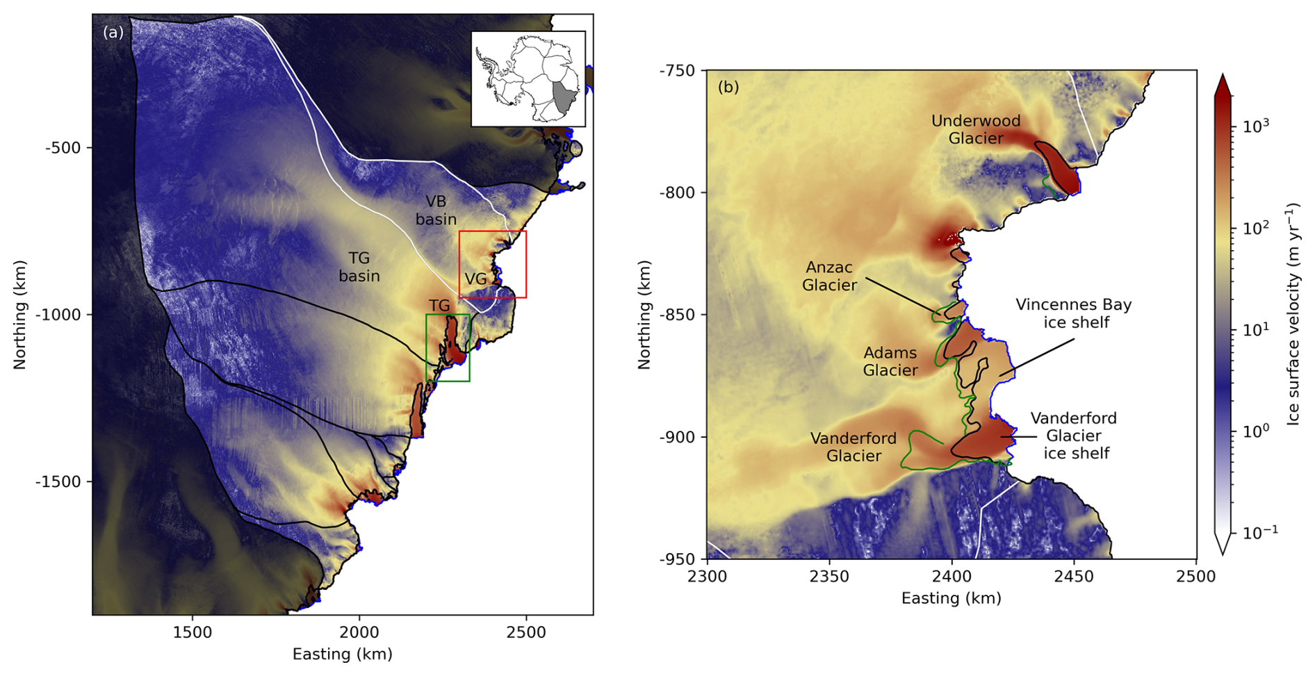
Figure 1 Overview of the Aurora Subglacial Basin, showing the Vincennes Bay drainage basin. (a) MEaSUREs v2 ice surface velocity (Rignot et al., 2017) for the Aurora Subglacial Basin. Black lines denote drainage divides and the MEaSUREs v2 grounding line from Mouginot et al. (2017). The model domain and Vincennes Bay drainage boundary are shown in white. Abbreviations are defined as follows: VG is Vanderford Glacier, TG is Totten Glacier, VB basin is Vincennes Bay drainage basin, and TG basin is Totten Glacier drainage basin. The red box indicates the extent shown in panel (b). The green box indicates the Totten Glacier extent shown in Fig. 2. (b) Vincennes Bay glaciers and ice shelves (Mouginot et al., 2017); all graphical components are consistent with panel (a). The Vanderford Glacier ice shelf is not explicitly defined by Mouginot et al. (2017); here we use “Vanderford Glacier ice shelf” to refer to the portion of the Vincennes Bay ice shelf that includes the main trunk of Vanderford Glacier. The 2020 grounding line is shown in green (Picton et al., 2023). The colour scale is consistent across panels (a) and (b).

Neighbouring the Vincennes Bay drainage basin, the Totten Glacier drainage basin is the largest catchment of the Aurora Subglacial Basin (Fig. 1). Totten Glacier has been losing mass at an increasing rate over recent decades and represents the largest East Antarctic contributor to sea level rise (Li et al., 2023a). McCormack et al. (2023) demonstrate the close relationship between Totten and Vanderford glaciers' flow configurations, suggesting that small changes to local ice geometry (e.g. potentially associated with changes in ice shelf buttressing at Vanderford Glacier due to ocean-driven thinning or calving) could result in the large-scale reconfiguration of ice flow and subglacial hydrology, having larger implications for ice dynamics across the Aurora Subglacial Basin. Vanderford Glacier appears to be currently grounded on a prograde bed slope limiting its retreat (Fig. 2c); however, bed topography in the region upstream of the grounding line is associated with > 500 m of uncertainty, which is some of the highest in East Antarctica (Morlighem et al., 2020). The region may be susceptible to marine ice sheet instability (MISI; Schoof, 2007; Weertman, 1974) under future warming conditions if extensive grounding line retreat into the upstream Aurora Subglacial Basin should occur.

Recent mass loss and grounding line retreat at Vanderford Glacier is believed to be linked to the intrusion of warm modified Circumpolar Deep Water (mCDW) into the ice shelf cavity via a deep marine trough offshore; however, high-resolution mapping of the trough extent across the continental shelf has not been conducted (Picton et al., 2023; McCormack et al., 2023). Basal melting in the region is likely dominated by mode-2 melting (Jacobs et al., 1992), where warm mCDW at depth drives melt close to the grounding line. This is consistent with the presence of the warmest recorded intrusions of mCDW in East Antarctica which have been observed in Vincennes Bay (Ribeiro et al., 2021; Herraiz-Borreguero and Naveira Garabato, 2022). The mCDW temperatures in Vincennes Bay are comparable to those at Totten Glacier, where mode-2 melting is dominant (Silvano et al., 2017, 2018; Ribeiro et al., 2021). However, recent satellite-derived basal melt estimates from Paolo et al. (2022) and Davison et al. (2023) show basal melt rates ranging from −9 to 34 m yr⁻¹ across the ice shelves within Vincennes Bay (Fig. 2a–b), compared to estimates of −8 to 67 m yr⁻¹ at Totten Glacier – up to twice those of Vincennes Bay, with high melt rates close to the grounding line (Fig. 2a–b). These disparate satellite-derived basal melt observations in neighbouring systems with similar offshore ocean properties suggest that basal melt rates in Vincennes Bay may be underestimated.

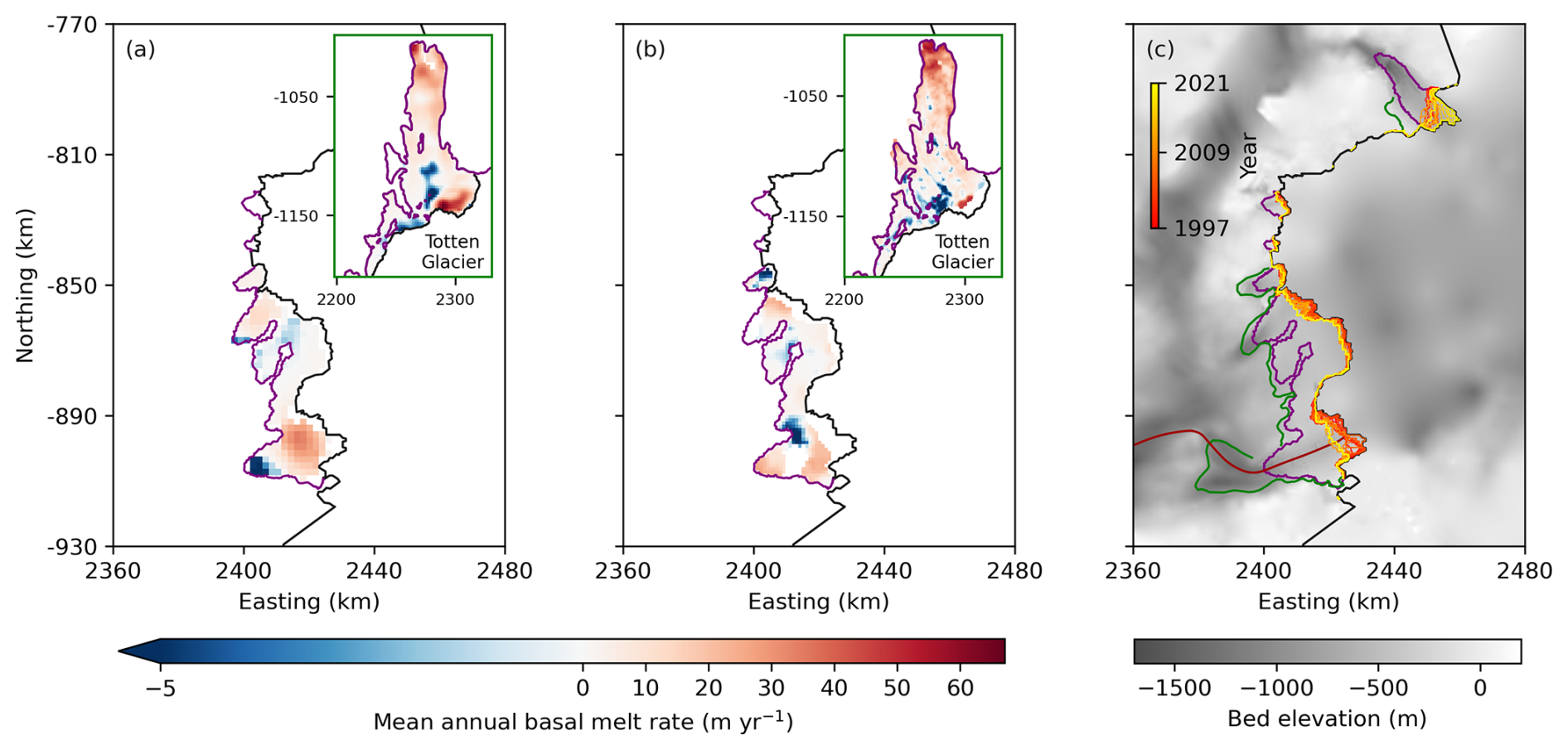
Figure 2 Sub-ice-shelf basal melt rates and ice front migration for Vincennes Bay. (a) Long-term mean annual basal melt rate derived from satellite altimetry (Paolo et al., 2022). (b) Long-term mean annual basal melt rate derived from satellite altimetry (Davison et al., 2023). (c) Ice shelf front positions from Greene et al. (2022), 2020 grounding line position (green line) from Picton et al. (2023), and Vanderford Glacier flowline along which grounding line retreat is measured (red line). Bed elevation is taken from BedMachine v3 (Morlighem et al., 2020). In all panels, the model domain extent is shown in black and the initial MEaSUREs v2 grounding line (Mouginot et al., 2017) in purple. The extent of the Totten Glacier inset in panels (a) and (b) is shown in Fig. 1a. No basal melt estimates are available for Underwood Glacier. For M_Paolo and M_Davison experiments, we interpolate these basal melt fields across the model mesh to ensure that basal melt rates are provided appropriately as grounding line migration occurs.

Recent work has also explored the influence of basal melt and calving on both the ice shelf mass budget (Davison et al., 2023) and changes in grounded ice discharge (Greene et al., 2022) for the Vincennes Bay region. Greene et al. (2022) model the instantaneous response to changes in floating ice geometry (calving and thinning) and show that changes in the ice front position account for approximately half of all Antarctic mass loss since 2007. For the Vincennes Bay region, Davison et al. (2023) show that calving dominated the freshwater fluxes (i.e. ice loss) from the ice shelf for the period of 1997 to 2021. However, to attribute relative contributions of basal melt and calving processes to mass loss relies on accurate predictions of basal melt. With no direct measurements of ice shelf melt in Vincennes Bay, basal melt estimates are derived at high resolution (i.e. 1 to 2 km) from satellite-altimetry-based methods; however, these methods require various simplifying assumptions that could lead to biases, particularly in small systems such as Vincennes Bay (Chartrand and Howat, 2023).

The sensitivity of Vanderford Glacier grounding line retreat and ice mass loss to different magnitudes of basal melt and calving perturbations has not been investigated, presenting a significant gap in our understanding of the region. Given the potential for broader implications across the Aurora Subglacial Basin arising from changes at Vanderford Glacier (McCormack et al., 2023), quantifying the relative contributions of these processes on grounding line retreat and mass loss is essential to better understanding the vulnerability of the region to a changing climate.

The aim of this study is to assess the sensitivity of mass loss and grounding line retreat at Vanderford Glacier to sub-ice-shelf basal melt and calving. We use time-evolving numerical ice sheet model simulations to address the following research questions: (1) can satellite-derived estimates of basal melt and ice front retreat generate the magnitude of observed grounding line retreat at Vanderford Glacier between 1996 and 2020; and, if not, (2) what magnitude of basal melt and/or calving is required to generate grounding line retreat of a similar magnitude to observations? Although the aim of this study is not to directly replicate recent trends at Vanderford Glacier, by addressing the above questions, we can infer the likely driver(s) of recent historical changes in mass loss and grounding line retreat at Vanderford Glacier.

This paper is structured as follows: in Sect. 2, we describe the ice sheet model set-up and initialisation process and provide an overview of our perturbation experiments. In Sect. 3, we present the results of our ice sheet model simulations, focusing on changes to key measures of mass loss and grounding line retreat; these results are discussed in Sect. 4. Finally, we provide a conclusion of this work in Sect. 5.

2 Data and methods

2.1 Ice sheet model set-up

We use the Ice-sheet and Sea-level System Model (ISSM; Larour et al., 2012) to run transient simulations of the Vincennes Bay drainage basin. The model domain (Fig. 1) covers the Vincennes Bay drainage basin from the MEaSUREs Antarctic Boundaries for International Polar Year (IPY) 2007–2009 v2 (Mouginot et al., 2017), extended to include the cumulative maximum ice shelf front extent from 1997 to 2021 from Greene et al. (2022). We use an anisotropic mesh comprising 95 156 elements with a variable resolution ranging from ∼ 150 m around the ice front of the Vincennes Bay ice shelf to a maximum resolution of ∼ 12 km in the interior of the basin, with a mean resolution of ∼ 590 m across the Vincennes Bay ice shelf and upstream of the grounding line. The initial grounding line is taken from the MEaSUREs Antarctic Boundaries for IPY 2007–2009 v2 (Mouginot et al., 2017). Bed topography and ice geometry are taken from BedMachine Antarctica v3 (Morlighem et al., 2020), and surface ice velocities are from MEaSUREs v2 (Fig. 1). We assume floating ice is in hydrostatic equilibrium. Due to the paucity of bathymetry estimates below floating ice, we adjust and smooth the bathymetry in the ice shelf cavity such that it deepens from the grounding line to the ice front, better reflecting the deep bathymetry offshore of the Vanderford ice front. The adjustment of the sub-ice-shelf bathymetry ensures that the ice shelf does not re-ground on unrealistic high points in the ice shelf cavity, introducing buttressing forces. We enforce a minimum water depth of 50 m below the ice shelf base and lower the bathymetry at the ice shelf front by 840 m, which is the mean difference between the BedMachine v3 bathymetry and multibeam swath bathymetry at the Vanderford Glacier ice front (Commonwealth of Australia, 2022). This approach may limit any grounding line advance across model simulations; however, the initial grounding line represents the most advanced grounding line since observations began; thus, we do not expect grounding line advance beyond this position. Furthermore, as the cavity geometry is not an explicit parameter in the basal melt parameterisation used here, deepening the bathymetry in the ice shelf cavity does not impact melt rates. For all model simulations, we use the two-dimensional shelfy-stream approximation (SSA) to the Stokes equations (MacAyeal, 1989).

Recognising the importance of the choice of basal friction law on ice mass loss estimates and grounding line dynamics (Brondex et al., 2017, 2019; Barnes and Gudmundsson, 2022), we consider different friction laws to account for the sensitivity of ice sheet models to different basal friction representations: Weertman (1974), Budd et al. (1979), and Schoof (2005), given respectively by

$$\begin{array}{}\text{(1)}& {\mathit{\tau }}_{\mathrm{b}}=C_{\mathrm{w}}^{\mathrm{2}}{\left|u_{\mathrm{b}}\right|}^{m-\mathrm{1}}{u}_{\mathrm{b}},\end{array}$$

$$\begin{array}{}\text{(2)}& {\mathit{\tau }}_{\mathrm{b}}=C_{\mathrm{b}}^{\mathrm{2}}N{u}_{\mathrm{b}}^{\mathrm{3}m},\end{array}$$

$$\begin{array}{}\text{(3)}& {\mathit{\tau }}_{\mathrm{b}}={\displaystyle \frac{C_{\mathrm{s}}^{\mathrm{2}}{\left|u_{\mathrm{b}}\right|}^{m-\mathrm{1}}}{{\left(\mathrm{1}+{\left(C_{\mathrm{s}}^{\mathrm{2}}/\left(C_{max}N\right)\right)}^{\mathrm{1}/m}\left|u_{\mathrm{b}}\right|\right)}^m}}{u}_{\mathrm{b}},\end{array}$$

where τ_b  (Pa)  is basal shear stress;  C_w  (kg${}^{\mathrm{1}/\mathrm{2}}$ m${}^{-\mathrm{2}/\mathrm{3}}$ s${}^{-\mathrm{5}/\mathrm{6}}$), C_b (s${}^{\mathrm{1}/\mathrm{2}}$ m${}^{-\mathrm{1}/\mathrm{2}}$), and C_s (kg${}^{\mathrm{1}/\mathrm{2}}$ m${}^{-\mathrm{2}/\mathrm{3}}$ s${}^{-\mathrm{5}/\mathrm{6}}$) are friction coefficients for the Weertman, Budd, and Schoof friction laws, respectively; u_b (m s⁻¹) is the basal velocity; m is a positive exponent set to $\mathrm{1}/\mathrm{3}$; and C_max is Iken's bound, set to 0.5 (Brondex et al., 2017). In Eqs. (2) and (3), N (Pa) relates to the effective pressure, calculated following Brondex et al. (2017), assuming a perfect hydrological connection between the subglacial hydrology system and the ocean, such that

$$\begin{array}{}\text{(4)}& N=\left\{\begin{array}{lcl}{\mathit{\rho }}_{\mathrm{i}}gH+{\mathit{\rho }}_{\mathrm{w}}g{z}_{\mathrm{b}}& \text{if}& z_{\mathrm{b}}<\mathrm{0},\\ {\mathit{\rho }}_{\mathrm{i}}gH& \text{if}& z_{\mathrm{b}}\ge \mathrm{0},\end{array}\right.\end{array}$$

where ρ_i is the ice density (917 kg m⁻³), g is the gravitational acceleration (9.81 m s⁻²), H is the ice thickness (m), ρ_w is the seawater density (1023 kg m⁻³), and z_b is the ice base elevation (m). We note that the system response to different friction laws is not the focus of this study; rather, we consider multiple friction laws to ensure that our findings are not dependent on a given representation of basal friction. We use a Glen-type flow relation (Glen, 1953) with a stress exponent of n = 3 and compute ice rigidity using inverse methods (Morlighem et al., 2013; Sect. 2.2). For all transient simulations, we use a 1-month time step, with sub-element grounding line (SEP1; Seroussi et al., 2014) and basal melt (SEM1; Seroussi and Morlighem, 2018) parameterisations. We provide constant surface mass balance forcing to the model using the 1991 to 2020 climate normal mean annual surface mass balance from RACMO2.3p2 reanalysis (van Wessem et al., 2018).

We limit our analysis to the region of the model domain that contributes to the Vincennes Bay and Anzac Glacier ice shelves (Fig. 1), principally for the purpose that this region is the primary focus of this study and these individual ice shelves become merged across all simulations. We quantify changes in grounding line position by measuring its migration along a central flowline in the main trunk of Vanderford Glacier (Fig. 2c). The Underwood Glacier to the west (Fig. 1) is outside of our area of interest and shows a relatively persistent grounding line location throughout all simulations. For this reason, we do not consider the response of Underwood Glacier in this study.

2.2 Ice sheet model initialisation

We invert ice rigidity and the basal friction coefficient for each friction law independently (Fig. 3), minimising a cost function which includes terms for the linear and logarithmic misfit between simulated and observed surface ice velocities (Morlighem et al., 2013). We first invert for ice rigidity over floating ice, selecting linear and logarithmic cost function coefficients such that the contributions to the total cost function are similar. For the basal friction inversion using the Budd friction law, we choose coefficients such that their contributions to the total cost function have the same order of magnitude (e.g. Morlighem et al., 2013). For the Schoof and Weertman friction laws, we choose cost function coefficients that yield similar area-weighted RMSE velocity misfits to the Budd friction law while minimising the velocity misfit across the domain. Finally, we invert for ice rigidity across the whole domain using consistent cost function coefficients across all friction laws such that the linear and logarithmic cost function contributions have the same order of magnitude. To penalise sharp gradients in the resultant fields, we add Tikhonov regularisation to all inversions, using L-curve analysis (Hansen, 2000) to determine the optimal regularisation parameters. Following the inversion process, the area-weighted RMSE velocity misfits for the Budd, Schoof, and Weertman friction laws are 8.2, 9.9, and 8.4 m yr⁻¹, respectively. All spatially varying basal friction and ice rigidity fields are held constant for the duration of all simulations.

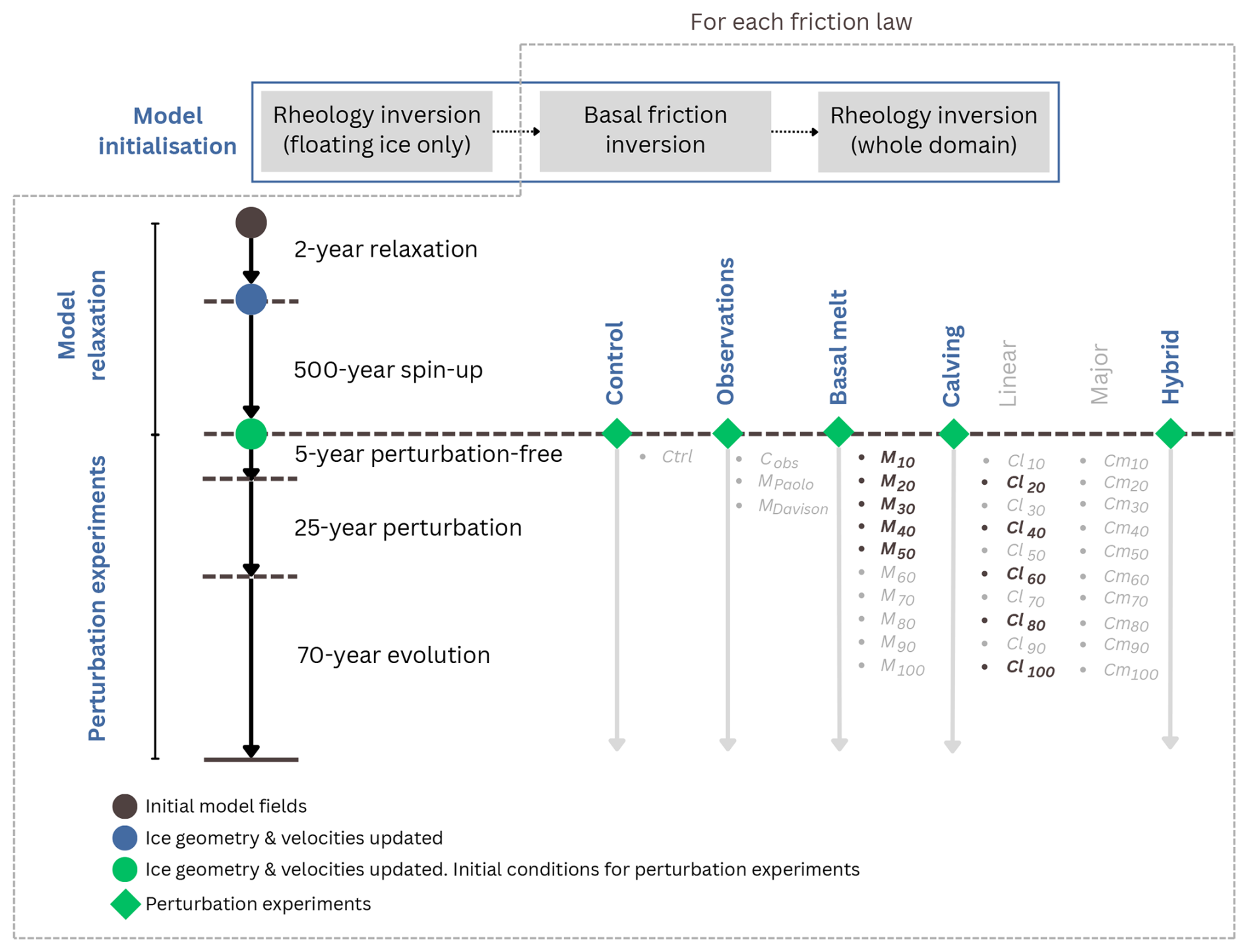
Figure 3 Overview of study methodology. Steps contained within the grey dotted boundary are completed independently for each friction law. Experiment names in bold indicate basal melt and calving processes combined in hybrid experiments.

Following model initialisation, we hold the grounding line fixed and perform an initial 2-year relaxation (Fig. 3) for each friction law to remove non-physical artefacts that result from observational uncertainties and discrepancies between data product epochs. Subsequently, we perform a 500-year spin-up simulation (Fig. 3) for each friction law where the grounding line is allowed to freely evolve. For this simulation, we prescribe a baseline basal melt rate (M) of 3 m yr⁻¹ across floating ice. We use 3 m yr⁻¹ as it is the median value of the two-dimensional long-term mean annual melt rate field across ice shelves within Vincennes Bay from Paolo et al. (2022). At the end of this 500-year simulation, ice velocities and geometry are in pseudo-steady state (Fig. S1 in the Supplement), and these fields are used as the initial conditions for all perturbation experiments (Sect. 2.3).

2.3 Perturbation experiments

To assess the sensitivity of Vanderford Glacier to sub-ice-shelf basal melt and calving, we perform a series of perturbation experiments, which run for 100 years, for each of the basal friction laws (Sect. 2.1). After an initial perturbation-free 5-year period using the same constant basal melt rates as in the spin-up, perturbations to either the basal melt rates or calving fronts are applied for 25 years, consistent with the time period over which recent grounding line retreat has been observed at Vanderford Glacier. At the end of the 25-year perturbation period, the model is allowed to evolve for an additional 70 years, again using the same constant forcings applied during the spin-up simulation. This approach allows us to quantify the instant and evolving ice sheet response to a perturbation. We also simulate a 100-year perturbation-free control simulation (Ctrl) where the forcings are consistent with the spin-up simulation. The system response to the control experiment is subsequently removed from all perturbation experiments to isolate the effect of each perturbation.

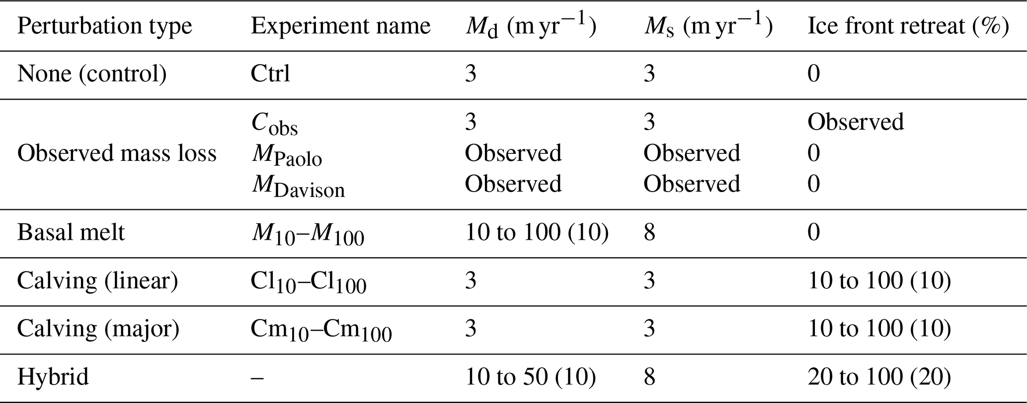
Beyond investigating the system response to observed conditions, we include basal melt and calving perturbation outside the observed range. These perturbation experiments are intended to capture the full range of plausible conditions, allowing us to assess the relative influence of varying magnitudes of perturbations of different mass loss drivers (i.e. basal melt and calving) on Vanderford Glacier. Perturbation experiments are broadly separated into four categories as follows and are summarised in Fig. 4 and Table 1:

• Observed mass loss experiments assess the response of the system to observed basal melt and calving (C_obs). To simulate the impact of observed basal melt, we use long-term mean annual basal melt rates (i.e. two-dimensional fields) derived from satellite altimetry for the period 1992 to 2017 from Paolo et al. (2022) (M_Paolo; Fig. 2a) and for the period 1997 to 2021 from Davison et al. (2023) (M_Davison; Fig. 2b). To simulate the impact of observed changes in the ice front, we use a time series of approximately annual ice front positions for the ice shelves across Vincennes Bay between 1997 and 2021 from Greene et al. (2022) (Fig. 2c). For M_Paolo and M_Davison experiments, we hold the ice front fixed and hold long-term mean annual melt rates constant across the perturbation period. For C_obs we include the baseline basal melt rate of 3 m yr⁻¹, consistent with the control simulation, and vary the ice front position using ice masks from Greene et al. (2022). We apply calving events annually on 1 January. There are only 24 ice masks included in the Greene et al. (2022) dataset, so we apply these annually from the beginning of the perturbation period and hold the ice front fixed following the final calving event. We note that the initial ice front extent used in C_obs simulations is the cumulative maximum ice front extent (consistent with the control simulation); thus, the magnitude of the initial calving event to reach the initial ice front extent from Greene et al. (2022) is likely larger than observed events.

• Basal melt perturbation experiments vary the magnitude of basal melt rates applied using a simple linear parameterisation, increasing melt rate with depth, such that

  $$\begin{array}{}\text{(5)}& M=\left\{\begin{array}{lcl}{M}_{\mathrm{s}}& \text{if}& z_{\mathrm{b}}\ge -\mathrm{300},\\ M_{\mathrm{d}}& \text{if}& z_{\mathrm{b}}\le -\mathrm{600},\end{array}\right.\end{array}$$

  where M_s is set to 8 m yr⁻¹ across all experiments and represents the area-weighted long-term mean annual melt rate from Paolo et al. (2022) and Davison et al. (2023) across regions with ice drafts ≥ −300 m. M_d varies between experiments by increments of 10 m yr⁻¹, from 10 to 100 m yr⁻¹, and the ice front is held fixed. Shallow and deep ice draft values (Eq. 5) are selected based on the depths of mCDW recorded within Vincennes Bay (Ribeiro et al., 2021). Basal melt rates applied to our simulations are shown in Fig. 4a.

• Calving experiments adjust the ice front to simulate calving processes. Two different mechanisms of ice front retreat (IFR) are tested, including continual linear retreat (Cl), intended to simulate edge wasting, and larger calving events occurring on a 12.5-year cycle (Cm) such that three large-scale calving events occur within the perturbation period. The choice of a 12.5-year calving cycle is arbitrary but is intended to represent larger discrete calving events. The final extent of IFR is consistent for Cl and Cm experiments and is determined as a percentage of the distance from the mean grounding line across all friction laws to the initial ice front in the along-flow direction. We vary the magnitude of IFR by increments of 10 %, from 10 % to 100 %. Baseline basal melt is included, consistent with the control simulation. We hold the ice front fixed at the final location following the perturbation period. Final ice front positions for each calving perturbation are shown in Fig. 4b.

• Hybrid experiments combine basal melt and calving processes, described above. We explore the combined effects of basal melt and calving to determine whether comparable system responses can be generated through multiple experimental set-ups. Here, we test a subset of basal melt and calving perturbations, including IFR values of 20 % to 100 % in increments of 20 % and M_d rates of 10 to 50 m yr⁻¹ in 10 m yr⁻¹ increments. We complete these hybrid experiments using only the linear calving mechanism (Cl). We compare the results against the corresponding basal melt perturbation without IFR to directly assess the effect of including IFR. We assess changes only at the end of the perturbation period.

For C_obs, Cl, and Cm experiments, we use the level-set method (Bondzio et al., 2016) to explicitly define ice front positions for each time step, based on observations for C_obs (Fig. 2c) and idealised ice front positions for Cl and Cm (Fig. 4b). The level-set method involves providing a two-dimensional field for each time step, defining regions of ice presence (negative values) and absence (positive values), where the zero contour defines the ice front. We assess the relative change in the perturbation experiments compared to the control experiment (Ctrl) for the following variables: grounding line flux (GL_flux), grounding line position, ice volume, and volume above floatation (VAF).

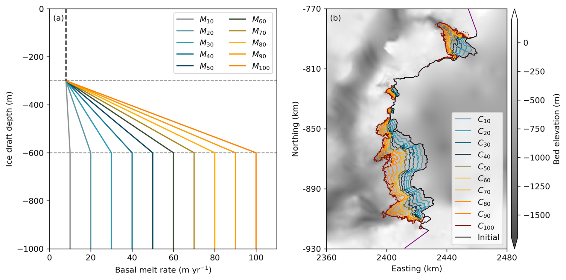
Figure 4 Overview of basal melt and calving perturbations. (a) Linear basal melt parameterisation. Vertical dashed black line represents constant M_s across all experiments. Horizontal dashed lines denote shallow (≥ −300 m) and deep (< −600 m) ice drafts where changes in M_d are applied. Note that the y axis is truncated at −1000 m for visualisation; however, basal melt rates are applied across all ice drafts. (b) Final ice front positions for all calving (Cl and Cm) perturbations. Note that final ice front positions are held constant following the perturbation period. The 100 % IFR perturbation varies depending on the friction law due to the specific grounding line location – Budd (solid), Schoof (dashed), and Weertman (dotted) – although differences are very minor and 100 % IFR lines plot on top of each other in panel (b). The purple outline denotes the model domain boundary. Ice front positions are plotted over bed elevation from BedMachine v3 (Morlighem et al., 2020).

Table 1 Overview of perturbation experiment forcings. Values in parentheses denote the increments of applied forcings across experiments. M_d is deep ice draft basal melt rate, and M_s is shallow ice draft basal melt rate. Subscripts used in experiment names for basal melt perturbations denote the corresponding M_d value. Subscripts used in experiment names for the calving perturbations denote the corresponding IFR percentage. No specific experiment names are assigned to hybrid experiments.

3 Results

We assess the results for each set of perturbation experiments individually. For each, we first consider the system response during the perturbation period and then the evolution following the perturbation period. We then consider the influence of the basal friction law during the perturbation period, followed by its influence on the evolution of the system after the perturbation period. The results of the observed mass loss perturbation experiments (M_Paolo, M_Davison, and C_obs) are presented in Sect. 3.1. Basal melt perturbation experiment results are shown in Sect. 3.2, calving perturbation experiments in Sect. 3.3, and hybrid experiments in Sect. 3.4.

3.1 Observed mass loss perturbations

None of the observed mass loss experiments results in marked changes in GL_flux, VAF, or grounding line position at any time throughout the simulations (Figs. 5a and e and 6a–c). The M_Davison experiment with the Weertman friction law shows rapid grounding line retreat of ∼ 2.5 km (Fig. 6b); however, this arises due to minimal ungrounding of a localised area and is not indicative of notable or widespread grounding line retreat. Ice re-grounds rapidly once the perturbation is removed (Fig. S2). Most mass loss occurs directly from the ice shelf rather than thinning or increased discharge of upstream grounded ice (Figs. 6c–d and S3). The C_obs experiment resulted in greater mass loss than both the M_Paolo and M_Davison experiments (Fig. 6d).

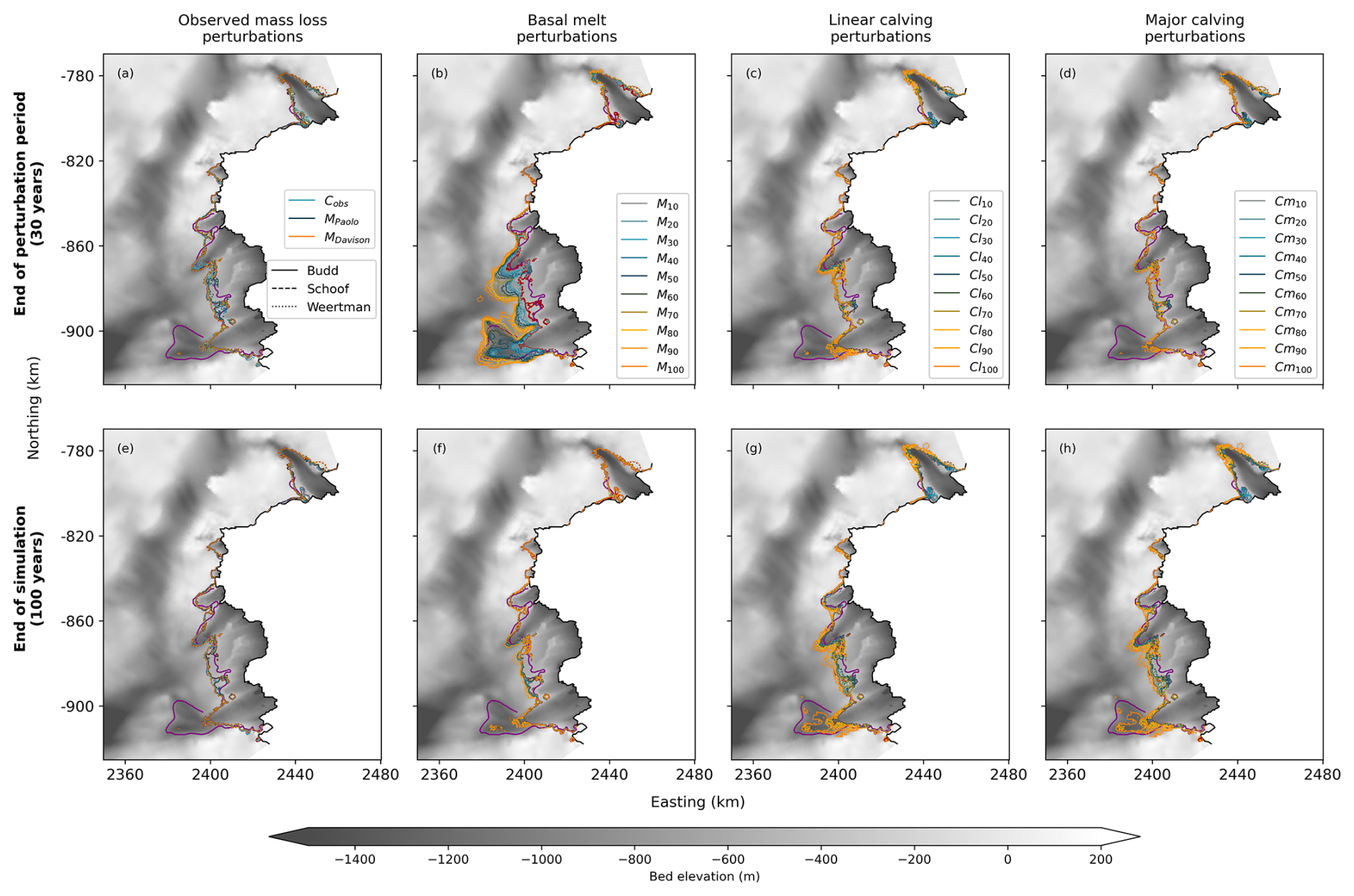
Figure 5 Grounding line positions across all perturbation experiments. (a–d) Grounding line positions at the end of the perturbation period (30 years). (e–h) Grounding line positions at the end of the simulation (100 years). Panels (a) and (e) show observed mass loss simulations, panels (b) and (f) show basal melt perturbations, panels (c) and (g) show linear calving (Cl) perturbations, and panels (d) and (h) show major calving (Cm) perturbations. Grounding lines in red show the initial grounding line for each simulation. The 2020 observed grounding line (Picton et al., 2023) is shown in purple. Bed elevation shows BedMachine v3 (Morlighem et al., 2020) bed topography and adjusted bathymetry below floating ice, used within our model. The black line is the initial ice front and the white line the domain boundary.

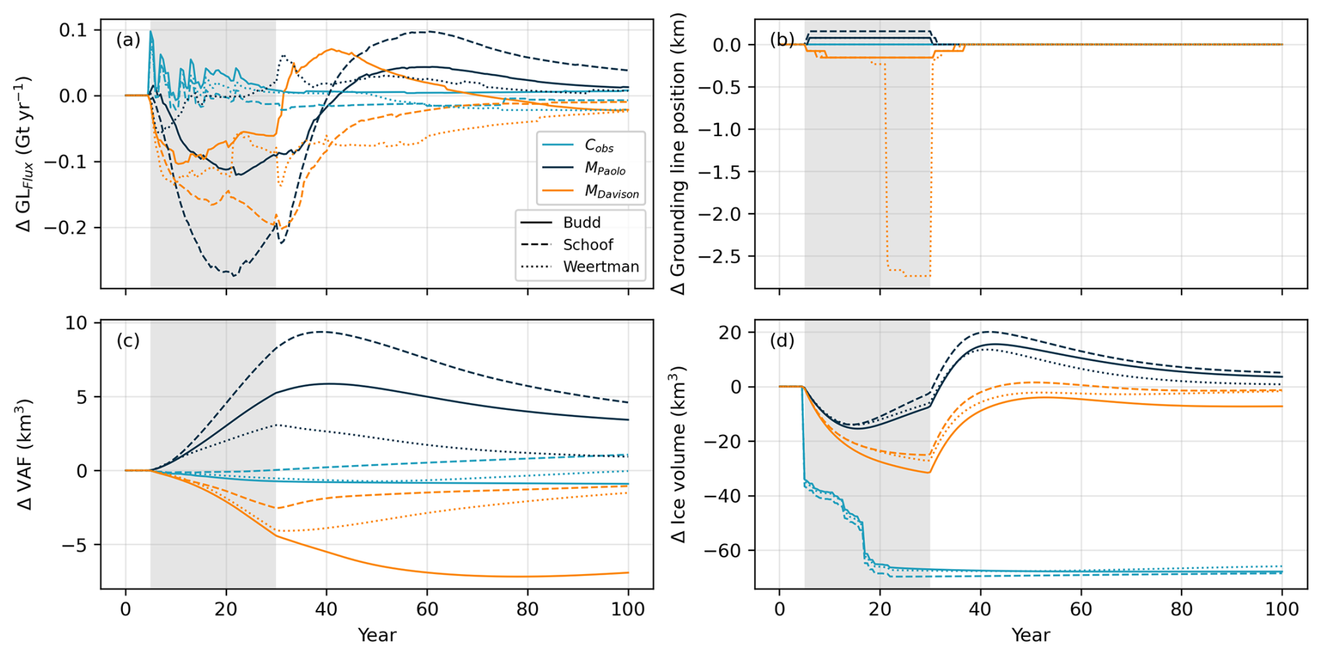
Figure 6 Results of observed mass loss perturbations. Relative change (compared to the Ctrl experiment for each friction law) of (a) grounding line flux and (b) grounding line retreat along the central flowline shown in Fig. 2c. Negative numbers represent grounding line retreat and positive numbers represent grounding line advance, relative to the Ctrl experiment. (c) Volume above floatation and (d) ice volume. Grey shaded area denotes the perturbation period.

During the perturbation period, the M_Paolo and M_Davison experiments show similar responses across all variables, except for VAF where the M_Paolo experiment shows an increase and the M_Davison experiment shows a decrease (Fig. 6c). Negative basal melt rates (i.e. ice accretion) in the M_Paolo experiment cause slight ice shelf thickening close to the Vanderford Glacier grounding line compared to widespread ice shelf thinning simulated in the M_Davison experiment (Fig. S3). Each experiment (C_obs, M_Paolo, and M_Davison) shows a pattern of change in VAF and ice volume that is generally consistent across friction laws, with differences in the magnitude of the change. For example, the M_Paolo experiment shows the largest range of VAF changes, from 3.0 to 8.3 km³ between the friction laws. Changes in GL_flux are negligible for all experiments (C_obs, M_Paolo, and M_Davison), but there are small variations in GL_flux (i.e. on the order of 0.2 Gt yr⁻¹) between the friction laws.

Following the perturbation period, all fields in the M_Paolo experiment trend towards their initial state, irrespective of the friction law. By the end of the simulation, VAF and ice volume remain elevated from their initial state due to thickening of grounded ice (Fig. S4). The M_Davison experiment with the Budd friction law shows continued mass loss, while the Schoof and Weertman friction laws show a tendency for ice volume to trend towards its initial state (Fig. 6c–d). The different response of the Budd friction law between M_Paolo and M_Davison is attributed to more widespread thinning of ice upstream of the grounding line (Fig. S4). The C_obs experiment shows no increase in ice volume due to the persistence of the final retreated ice front compared to the initial location (Fig. 6d).

Overall, the system shows a negligible response when perturbed with observed basal melt and calving events. There is minor variability between friction laws, and most notable changes in VAF and ice volume result from disparities in basal melt estimates, particularly close to the grounding line.

3.2 Basal melt perturbations

Over the perturbation period, all basal melt experiments yield an increase in GL_flux, ice volume loss, and grounding line retreat (Figs. 5b and 7). Grounding line retreat into regions of deeper bed topography, where increased ice velocities dominate over the general thinning of upstream ice, leads to increased GL_flux (Fig. 7a). Ice volume loss and GL_flux increase linearly with M_d values > 50 m yr⁻¹. All experiments show a decrease in VAF (Fig. 7g), consistent with dynamic thinning of grounded ice upstream of the grounding line (Figs. S5a and S6). For M_d values ≤ 50 m yr⁻¹, our experiments suggest maximum grounding line retreat of 9.7 km, while M_d values > 50 m yr⁻¹ lead to grounding line retreat within the range of observed retreat (15.2–21.7 km).

Following the perturbation period, all experiments show grounding line re-advance, with the final grounding line position close to the initial location (Figs. 5f and 7d). The VAF continues to reduce for a period of ∼ 30 years, consistent with continued thinning upstream of the grounding line (Fig. S5a). Total ice volume increases from the end of the perturbation period resulting from ice shelf thickening (Fig. S5d). The GL_flux reduces as a result of persistent thinning upstream of the grounding line which is not offset by sufficiently large and sustained magnitude changes in velocity (Figs. S5a and g).

During the perturbation period, the pattern of system response is similar for all friction laws, but the magnitude differs. The Weertman friction law generally yields the smallest change in GL_flux. For M_d values ≤ 50 m yr⁻¹, the Weertman friction law shows more extensive grounding line retreat than the other friction laws; however, for M_d values > 50 m yr⁻¹ the Budd friction law causes more extensive grounding line retreat. Ice volume at the end of the perturbation period does not show a clear relationship with the choice of friction law, with each yielding a similar response.

Following the perturbation period, the choice of friction law plays a key role in the rate and magnitude of ice volume evolution (Fig. 7g and j). The Budd friction law consistently yields the smallest rate of ice volume increase due to higher-magnitude dynamic thinning upstream of the grounding line following the perturbation period (Fig. S5a). The Weertman friction law consistently yields the highest rate of ice volume increase.

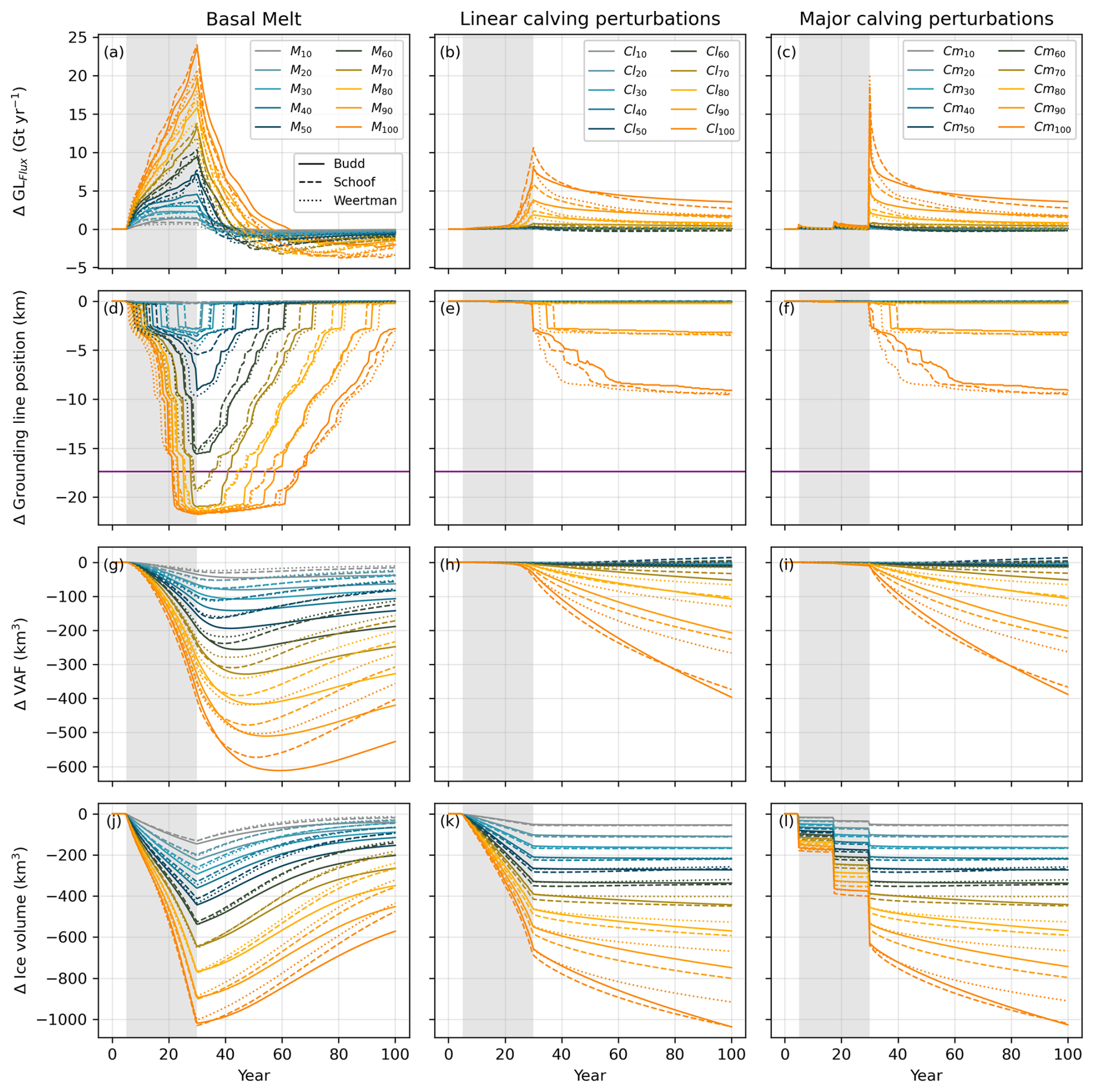
Figure 7 Results of basal melt and calving perturbations. Relative change (compared to the Ctrl experiment for each friction law) of (a–c) grounding line flux and (d–f) grounding line retreat along the central flowline shown in Fig. 2c. Negative numbers represent grounding line retreat and positive numbers represent grounding line advance, relative to the Ctrl experiment. (g–i) Volume above floatation and (j–l) ice volume. Basal melt (M) perturbations are shown in the first column, linear calving (Cl) perturbations in the second, and major calving (Cm) perturbations in the third. Grey shaded area denotes the perturbation period. The horizontal purple line in panels (d)–(f) shows the location of the 2020 grounding line (Picton et al., 2023), along the central flowline shown in Fig. 2c, relative to the mean grounding line location across all three basal friction Ctrl experiments.

Overall, the system shows a similar pattern of response to all basal melt perturbations and all friction laws, with an increased magnitude of response as M_d increases. Values of M_d > 50 m yr⁻¹ are required to generate grounding line retreat close to the observed grounding line location, which is much larger than current estimates of basal melt (Fig. 2a–b).

3.3 Calving perturbations

Over the perturbation period, all calving experiments yield an increase in GL_flux and ice volume loss, irrespective of the calving mechanism (Cl or Cm). Changes in VAF are minimal, highlighting that mass loss predominantly occurs from floating ice in both Cl and Cm experiments (Fig. 7h and i). Major calving (Cm) experiments show an instantaneous response in GL_flux (Fig. 7c) and ice volume (Fig. 7l) to calving events which occur at 12.5-year intervals (5, 17.5, and 30 years), while linear calving (Cl) experiments show a more gradual response (Fig. 7b and k). The magnitude of GL_flux increase is negligible, and no grounding line retreat occurs for all experiments with < 80 % IFR (i.e. Cl₁₀–Cl₇₀ and Cm₁₀–Cm₇₀; Figs. 5c–d and 7e–f). Notable grounding line retreat only occurs towards the end of the perturbation period for the experiments with 100 % IFR (i.e. ice shelf removal). The Cl experiments show slightly earlier onset and marginally larger magnitude grounding line retreat compared to the Cm experiments (Fig. 7e–f).

Following the perturbation period, GL_flux reduces but remains elevated from its initial state for all experiments with ≥ 80 % IFR due to increased velocities and dynamic thinning upstream of the grounding line (Fig. S5b–c and h–i). The Cl and Cm experiments with < 80 % IFR show negligible additional change in ice volume or VAF, while experiments with ≥ 80 % IFR show continued ice volume loss, consistent with the persistent increased GL_flux. Grounding line retreat continues for all experiments with ≥ 80 % IFR, with only minor retreat (< 1 km) for Cl₈₀ and Cm₈₀ and a maximum retreat of ∼ 9 km for the Cl₁₀₀ and Cm₁₀₀ experiments (Figs. 5g–h and 7e–f).

During the perturbation period, the pattern of the system response is similar for all friction laws, but the magnitude differs. The Schoof friction law consistently yields the largest mass loss (Fig. 7k–l). The magnitude of grounding line retreat is similar between all experiments, with the Weertman friction law leading to greater retreat for experiments with 90 % and 100 % IFR. For Cl and Cm experiments with ≥ 80 % IFR, the Schoof friction law yields a greater GL_flux.

Following the perturbation period, GL_flux reduces but remains elevated for all Budd friction law experiments and Schoof and Weertman friction law experiments with ≥ 80 % IFR (Fig. 7b–c). The Budd friction law consistently yields the highest GL_flux at the end of the simulation. The Weertman friction law generally yields the largest ice volume at the end of the simulation period, while the Budd and Schoof friction laws generate more varied results (Fig. 7k–l). Continued grounding line retreat is generally consistent between all experiments, with the Schoof friction law generating marginally larger retreat for experiments with ≥ 80 % IFR (Figs. 5g–h and 7e–f).

The mechanism of calving (i.e. Cl or Cm) primarily affects the response of the system over the perturbation period, particularly changes in GL_flux. We compare the absolute cumulative change in GL_flux between Cl and Cm experiments following large-scale calving events and at the end of the simulation period (i.e. at 5, 17.5, 30, and 100 years) to directly compare the influence of the calving mechanism on dynamic mass loss (Fig. 8). Figure 8 shows the similarity of the absolute cumulative change in GL_flux between Cl and Cm calving perturbations. After the initial major calving event (5 years), the mean (i.e. across all experiments and friction laws) absolute cumulative change in GL_flux from Cm experiments (0.14 ± 0.09 Gt yr⁻¹) is several magnitudes larger than Cl experiments ($\mathrm{3}\times {\mathrm{10}}^{-\mathrm{5}}$ ± $\mathrm{1}\times {\mathrm{10}}^{-\mathrm{5}}$), primarily due to negligible changes in GL_flux for Cl experiments and larger-magnitude instantaneous changes for Cm experiments. At the next major calving event (17.5 years), the mean absolute cumulative change in GL_flux from Cm experiments (2.35 ± 1.65 Gt yr⁻¹) is 14 % larger than from Cl experiments (2.06 ± 1.38 Gt yr⁻¹). Subsequently, at the next major calving event (30 years) Cl experiments yield a mean absolute cumulative change in GL_flux (14.66 ± 18.97 Gt yr⁻¹) that is 92 % larger compared to Cm experiments (7.64 ± 7.31 Gt yr⁻¹). At the end of the simulation period, the mean absolute cumulative change in GL_flux from Cl experiments (119 ± 196 Gt yr⁻¹) is < 1 % larger than that from Cm experiments (118 ± 195 Gt yr⁻¹).

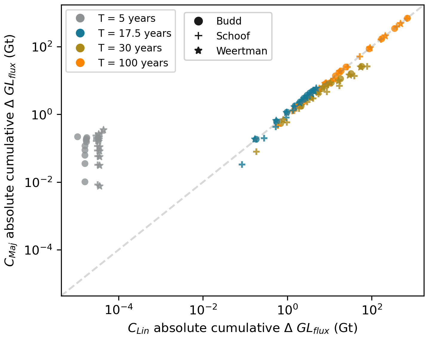
Figure 8 Comparison of absolute cumulative relative change (compared to the Ctrl experiment for each friction law) in grounding line flux between Cl and Cm experiments at select time steps throughout the simulation period.

Overall, while the calving mechanism (Cl or Cm) affects the instantaneous response of the system, there is a similar response across Cl and Cm experiments over the 100-year simulation period. IFR of ≥ 80 % is required to generate any notable system response which is much larger than observed IFR (Fig. 2c).

3.4 Hybrid experiments

Section 3.2 and 3.3 show that M_d values > 50 m yr⁻¹ are required to generate grounding line retreat close to the observed position and that calving processes yield negligible grounding line retreat until ≥ 80 % IFR occurs. Here, we explore whether combined lower-magnitude basal melt and calving perturbations can generate a comparable system response. The addition of IFR to low-magnitude basal melt processes has a negligible effect on GL_flux or grounding line position until ≥ 80 % IFR has occurred (Fig. 9), consistent with the effects shown in Sect. 3.3.

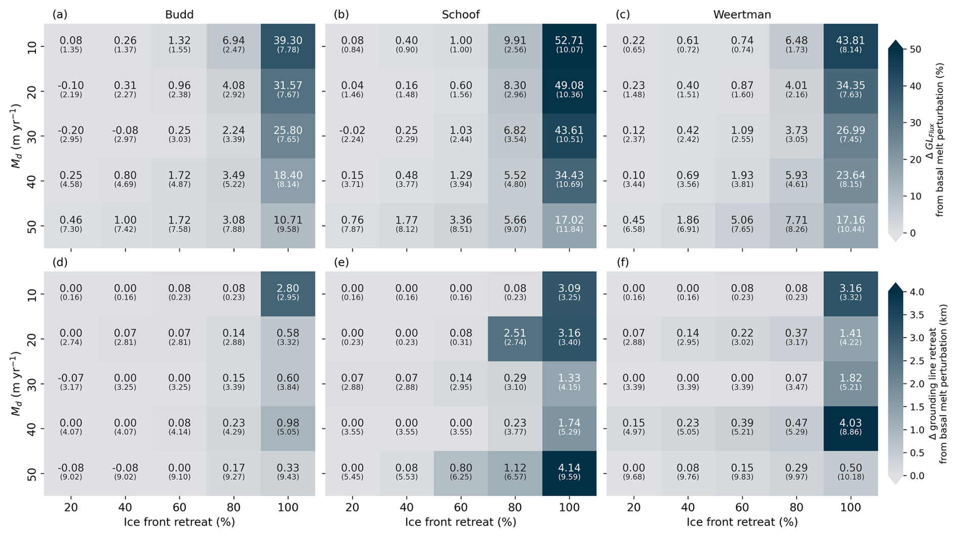
Figure 9 Influence of IFR on GL_flux and grounding line retreat when combined with basal melt. (a–c) Change in GL_flux and (d–f) change in grounding line retreat. The colour scale and large font numbers display changes relative to the corresponding basal melt perturbation for each friction law as per the colour-scale label. Values in parentheses show the absolute relative change in each variable compared to the control experiment. For example, the Budd friction law experiment with M_d = 40 m yr⁻¹ and 100 % IFR shows that including IFR produces an 18.40 % increase in GL_flux, compared to the M₄₀ basal melt perturbation, and the combined experiment yields an 8.14 Gt yr⁻¹ increase in GL_flux relative to the Budd control experiment.

The relative change in GL_flux due to IFR generally shows an inverse relationship with M_d for experiments with ≥ 80 % IFR (Fig. 9a–c). We attribute this to the relative increase in direct mass loss from the ice shelf decreasing with M_d, resulting in reduced buttressing forces; i.e. ice shelf thickness is generally inversely related to M_d such that less mass is removed over an equivalent area of calving as ice thickness decreases. For experiments with ≥ 80 % IFR, the Schoof friction law generally results in the largest increase in GL_flux, while the Budd friction law generally yields the smallest (Fig. 9a–c). For example, for the hybrid experiment with M_d = 50 m yr⁻¹ and 100 % IFR, the Schoof friction law results in a ∼ 6 % greater influence (17 % increase in GL_flux) compared to the Budd friction law (∼ 11 % increase in GL_flux).

The effect of including IFR on grounding line retreat shows no clear pattern, with the greatest retreat occurring for different M_d values across different friction laws. The Schoof friction law generally results in more consistent and larger-magnitude grounding line retreat across all experiments (Fig. 9d–f). However, none of the experiments yields grounding line positions close to the observed position by the end of the perturbation period (see absolute values shown in Fig. 9d–f).

While the addition of IFR to basal melt perturbations generally results in increased GL_flux and additional grounding line retreat, the influence is insufficient to generate sufficient additional grounding line retreat required to match the observed grounding line position. Thus, as in the standalone basal melt experiments, high basal melt rates at depth (i.e. M_d > 50 m yr⁻¹) are required to simulate grounding line retreat similar to that observed.

4 Discussion

This study examines the sensitivity of Vanderford Glacier to sub-ice-shelf basal melt and ice front retreat (IFR). When forced with current observational estimates of calving and basal melt, our simulations do not generate grounding line retreat close to the present-day location over the perturbation period. This suggests that estimates of sub-ice-shelf basal melt rates from satellite altimetry (Paolo et al., 2022; Davison et al., 2023) may substantially underestimate basal melt, particularly close to the grounding line. A possible cause of this underestimation is the assumption of hydrostatic equilibrium (i.e. that ice is freely floating across the entire ice shelf) in methods to derive basal melt from satellite altimetry. In regions with steep ice thickness gradients (i.e. conducive to regions of heavy crevassing) and at shear margins, the validity of this assumption is challenged due to high strain rates and associated bridging stresses (e.g. Wearing et al., 2021; Chartrand and Howat, 2020, 2023; Dow et al., 2024). Chartrand and Howat (2023) investigate the effects of uncertainties in estimates of hydrostatic thickness on basal mass balance estimates for Antarctica, finding that the Vincennes Bay and Underwood ice shelves have some of the largest uncertainties in hydrostatic-thickness-derived basal melt rates in East Antarctica. These hydrostatic thickness uncertainties result in large uncertainties in basal mass balance estimates (−0.8 ± 12.7 m w.e. yr⁻¹) across Vincennes Bay, influenced largely by spatial changes in the strain rate across the ice shelves (Chartrand and Howat, 2023). We note that when accounting for the upper range of basal mass balance uncertainty, satellite-derived estimates of basal melt rates across the Vanderford Glacier ice shelf (Fig. 2a–b) are always below 50 m yr⁻¹. This suggests that uncertainties in hydrostatic thickness alone cannot explain the elevated basal melt required to drive grounding line retreat at Vanderford Glacier in our sensitivity analyses. This highlights the need for improved estimates of basal melt across ice shelves within Vincennes Bay. While recent advances in satellite-derived basal melt estimates (e.g. Shean et al., 2019; Paolo et al., 2022; Davison et al., 2023; Zinck et al., 2023) allow for high-resolution estimates of sub-ice-shelf basal melt, some simplifying assumptions (e.g. hydrostatic equilibrium) have limited applicability in small dynamic systems such as those across Vincennes Bay, which highlights the ongoing need for direct observations (e.g. geophysical or oceanographic) to help constrain remotely sensed estimates (McCormack et al., 2024).

We show that basal melt rates > 50 m yr⁻¹ at depth are required to generate grounding line retreat close to the present-day location over the perturbation period – approximately twice those of Paolo et al. (2022) and Davison et al. (2023). Importantly, our simulations show that the observed grounding line retreat at Vanderford Glacier is unlikely to result from calving, since grounding line retreat only occurs with ≥ 80 % IFR – a much larger-magnitude IFR than has been observed. In the absence of basal melting > 50 m yr⁻¹ at depth, even when the entire ice shelf is removed (Cl₁₀₀ and Cm₁₀₀), the magnitude and rate of simulated grounding line retreat are not comparable to observations. For example, it takes more than 95 years for Cl₁₀₀ experiments to generate a maximum grounding line retreat of ∼ 9 km. It is possible that the observed grounding line retreat could be in response to a major calving event prior to the satellite observational era; however, we believe this is unlikely due to the scale of the event that would be required to generate the observed retreat, the absence of other evidence conducive to previous ice shelf collapse (e.g. rapid changes in ice thickness and ice velocity), and the size of observed calving events in recent decades being of much smaller magnitude. Our results indicate that basal melting is the likely driver of recent grounding line retreat at Vanderford Glacier.

The melt rate parameterisation used in this study is a highly simplified representation of basal melting. While it captures the depth dependence of melt rates consistent with mCDW-driven melt, it neglects the role of subglacial discharge and ocean dynamics which are known to impact melt rates in the neighbouring Totten Glacier ice shelf (Gwyther et al., 2023; Xia et al., 2023) and may also play an important role in ice shelves across Vincennes Bay (Jacobs et al., 1992; Silvano et al., 2016). Importantly, spatial and temporal variations in thermocline depth, which are known to have implications for mode-2 melting (e.g. De Rydt et al., 2014; Dutrieux et al., 2014; Hoffman et al., 2019), are not captured by this melt rate parameterisation. Here, we select a thermocline depth based on the depth at which mCDW is predominantly found in Vincennes Bay (Ribeiro et al., 2021). Previous studies have shown a dynamic subglacial hydrology network beneath the Totten Glacier drainage basin (Dow et al., 2020), and ocean modelling of Totten ice shelf cavity shows that subglacial freshwater discharge from this network can enhance basal melting by over 3 % across the ice shelf, with localised increases of 25 % to 30 % in regions close to the grounding line (Gwyther et al., 2023). Although Dow et al. (2020) do not include the whole Vincennes Bay hydrological catchment in their analysis, there is evidence for an extensive subglacial hydrology system across the Aurora Subglacial Basin (Wright et al., 2012), potentially with strong connectivity between the Totten and Vanderford upstream catchments. Hence, similar localised convective plumes resulting from buoyant discharge of freshwater that enhance basal melting in the Totten Glacier ice shelf cavity may also play a strong role in basal melting in the Vanderford Glacier ice shelf cavity.

More complex basal melt parameterisations (e.g. PICO/PICOP and the ISMIP6 protocol; Reese et al., 2018; Pelle et al., 2019; Jourdain et al., 2020) rely on temperature and salinity forcing from regional ocean model output. However, known disparities in offshore bathymetry in Vincennes Bay may limit the accuracy of regional ocean models here, since they may not correctly represent local ocean conditions that may arise from bathymetric features. Specifically, the presence of the deep marine trough mapped offshore of Vanderford Glacier (Commonwealth of Australia, 2022) is absent in continental bathymetry estimates (e.g. BedMachine v3; Morlighem et al., 2020) commonly used within ocean models. This bathymetric feature could have important implications for ocean dynamics, potentially providing a pathway for mCDW into the Vanderford Glacier ice shelf cavity. Thus, without this feature, ocean models may underestimate basal melt in the Vanderford Glacier ice shelf cavity. Similarly, uncertainties in bed topography upstream of the grounding line could have implications for our simulated grounding line retreat, with deeper bed topography potentially resulting in more rapid or extensive grounding line retreat occurring with lower basal melt rates. This highlights the need for improved bathymetric mapping across Vincennes Bay to support more reliable ocean modelling and basal melt rate estimates, as well as additional geophysical data acquisition over grounded ice to improve bed topography estimates.

One of the consequences of the simplification in our melt parameterisation is a potentially spurious reconfiguration of ice flow; i.e. local changes in ice velocity across Vanderford Glacier ice shelf show a decrease in the strength of the western shear margin (Fig. S7) indicative of ice-flow reconfiguration based on changes in the driving stress. While shear margin migration has been found to induce grounding line retreat and promote mass loss (Feldmann et al., 2022; Lhermitte et al., 2020), observational records of ice velocity at Vanderford Glacier do not show this migration. We attribute this to our simulated melt rates in the region to the west of Vanderford Glacier likely being too high. We note that the ice flow trends towards its original configuration once the basal melt perturbation is removed and the ice shelf re-thickens.

Joughin et al. (2021) show that simulated mass loss at Pine Island Glacier exhibits only minor sensitivity (< 6 %) to melt distribution and depends linearly on the total melt. We test whether this is also the case for Vincennes Bay by running four additional experiments with constant melt rates of 10, 20, 30, and 40 m yr⁻¹ across all floating ice. We find that notable grounding line retreat towards the observed location requires constant melt rates of ≥ 30 m yr⁻¹ (Fig. S8). However, for melt rates > 10 m yr⁻¹, large portions of the ice shelf are completely removed (Fig. S8). This behaviour is not supported by observations, which may suggest that Vanderford Glacier grounding line retreat is driven by elevated basal melt at depth, consistent with observed mCDW intrusions within Vincennes Bay primarily located at 300–600 m depth (Ribeiro et al., 2021; Herraiz-Borreguero and Naveira Garabato, 2022).

Ocean modelling of future ice shelf basal melt around Antarctica shows that basal mass loss could increase by 33 % to 83 % in the Australian sector of East Antarctica by the end of the century (Naughten et al., 2018), depending on the future climate forcing scenario. Increased future mass loss projections suggest that continued grounding line retreat from reduced buttressing forces may be observed at Vanderford Glacier over the coming decades, consistent with findings from Sun et al. (2016). The current dominance of mCDW-driven melt may be reduced as Antarctic Surface Water becomes more prevalent with a reduction in future sea ice cover (Naughten et al., 2018). In turn, this could lead to melting dominated by mode-3 (i.e. surface-dominated) in the region in the future. Our experiments with a constant melt rate across the entire ice shelf suggest that a regime shift towards mode-3-dominated melt could increase mass loss from Vanderford Glacier as large portions of the ice shelf are removed with elevated melting across shallow ice regions (Fig. S8). More widespread mass loss from the ice shelf, beyond the region of passive ice, may lead to reduced buttressing forces and accelerated grounding line retreat.

Given the negligible effects of observed calving on simulated ice dynamics and grounding line position (i.e. experiment C_obs), it is likely that observed calving events have only removed passive ice (Fürst et al., 2016) from the calving front of the Vincennes Bay ice shelf. To confirm this, we compute the maximum buttressing field following Fürst et al. (2016) using the initial velocities at the beginning of our experiments (Fig. 10). The observed calving extent (i.e. Greene et al., 2022) does not extend beyond the 0.4 passive-shelf-ice threshold (Fürst et al., 2016) for the Vincennes Bay ice shelf. Our calving perturbation experiments suggest IFR ≥ 80 % is required to initiate non-negligible changes in ice dynamics at Vanderford Glacier. This behaviour is generally consistent with findings from Mitcham et al. (2022), in which an equivalent of ∼ 90 % IFR of the Larsen C ice shelf is required to generate a ∼ 50 % increase in the grounding line flux in their idealised calving experiments. Along the main trunk of Vanderford Glacier where most ice discharge occurs, the extent of 80 % IFR is similar to the 0.8 instantaneous discharge threshold contour, as defined for Vanderford Glacier by Fürst et al. (2016) (Fig. 10).

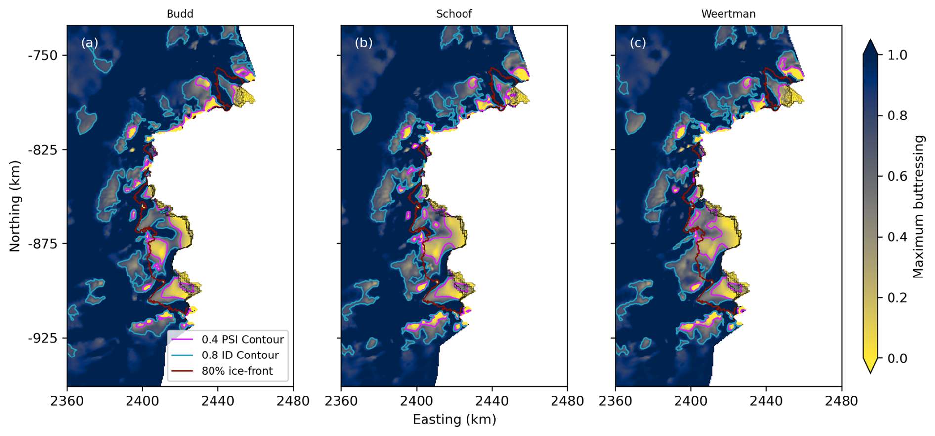
Figure 10 Maximum buttressing field calculated from initial velocities at the beginning of each perturbation experiment for each friction law: (a) Budd, (b) Schoof, and (c) Weertman. Black lines display the extent of the observed ice fronts from Greene et al. (2022). Maximum buttressing values are truncated between 0 and 1.

Our simulations show that the Vanderford Glacier system generally responds rapidly to calving events despite a more gradual response from Cl experiments and a more delayed response in grounding line retreat compared to basal melt experiments. The overall response is generally independent of the process by which calving occurs (i.e. edge wasting or major calving events). This may in part be due to the simplified implementation of calving used in our simulations; i.e. we have used a level-set method to prescribe the location of the ice front at each time step (Sect. 2.3), which does not capture the influence of transient changes in stress and strain fields across the ice shelf that may be better represented in more physically based calving laws (e.g. eigencalving or von Mises calving laws; Wilner et al., 2023). Furthermore, we hold the ice front at the final location (Fig. 4b) following the perturbation period, while in reality, additional re-advance of and calving from the ice front would occur. As such, our calving perturbations represent the worst-case impact of calving with a persistent retreated ice front such that the actual impacts of calving on grounding line retreat and mass loss are likely even smaller.

Our results show a varied response to different friction laws across the perturbation period and the whole simulation run, as well as between different variables we assess. In general, the Weertman friction law yields the smallest change in VAF across the simulation period, and the Budd friction law yields the largest changes. The magnitude and upstream extent of grounded ice thickness changes are largest for the Budd friction law (Fig. S6). The behaviour of the Budd friction law is attributed to the relationship between basal shear stress, effective pressure, and sliding velocities (Joughin et al., 2019; Brondex et al., 2017, 2019); i.e. in the Budd friction law, the basal shear stress is linearly proportional to the effective pressure such that as grounded ice thins, the effective pressure is lowered, basal shear stress is reduced, and sliding increases (Carr et al., 2024). This is not the case in either the Weertman friction law (where there is no explicit representation of basal water pressure) or the Schoof friction law (where effective pressure is controlled by cavitation) (Joughin et al., 2019).

Our finding of the Budd friction law yielding the largest changes in VAF is in agreement with previous studies for both idealised experiments (Brondex et al., 2017) and simulations of the Amundsen basin (Brondex et al., 2019). Despite variability in the magnitude of the response between different friction laws, our simulations show a similar response and trajectory throughout the simulation period. This is similar to findings from Barnes and Gudmundsson (2022), who show general consistency across their simulations of the Amundsen Sea Embayment for up to a century, suggesting that decadal- to centennial-scale simulations may be insensitive to the choice of friction law. We recognise that the choice of sliding law parameters is also shown to have important implications at similar timescales (Brondex et al., 2017, 2019; Barnes and Gudmundsson, 2022); however, assessing the sensitivity of the Vincennes Bay region to a full suite of basal friction representations is out of the scope of this study. Importantly, the presence of an active subglacial hydrology across the Aurora Subglacial Basin (Wright et al., 2012) likely means that these simple parameterisations of basal sliding will not represent the complex interactions at the ice–bed interface and that coupled subglacial hydrology and ice sheet model simulations are required to better understand the influence of basal sliding on the evolution of the Vincennes Bay region.

Our choice of model initialisation and spin-up to pseudo-steady state directly addresses the study aim and ensures that the system responds only to the instantaneous perturbation applied to the different forcings and is not influenced by any inertia or trends within the system. This approach allows us to untangle the changes in grounding line flux, grounding line migration, volume above floatation, and ice volume that arise from basal melt and ice front retreat, independently and in combination. Importantly, this approach limits our ability to comment on the current state of Vanderford Glacier (i.e. whether or not it may be undergoing irreversible grounding line retreat). To accurately assess the current state or to comment on potential future behaviours at Vanderford Glacier, additional modelling simulations which use a present-day model initialisation (i.e. to accurately match recent trends in mass loss and spatial patterns of ice thickness, ice velocity, and grounding line position) are recommended. Simulations of present-day behaviour require improved observations of basal melt, particularly close to the grounding line, and a more accurate representation of bathymetry in ocean models used to parameterise sub-ice-shelf basal melt is needed to support simulations of future behaviour.

5 Conclusions

In this study, we explore the relative importance of basal melt and calving on grounding line retreat at Vanderford Glacier and assess whether current estimates of mass loss can explain observed grounding line retreat. We found that basal melt rates > 50 m yr⁻¹ at depth are required to generate grounding line retreat close to observations over the 25-year perturbation period. Although this may be an overestimation of actual basal melt rates required to drive observed grounding line retreat (due to the simplified basal melt parameterisation used in this study), our findings show that it is likely ocean-driven melt that is responsible for recent observed grounding line retreat and not calving. Simulations using observational datasets of basal melt and calving do not result in grounding line retreat close to observations over the perturbation period, suggesting that satellite altimetry datasets may substantially underestimate melt at Vanderford Glacier. Our idealised calving experiments show that complete ice shelf removal is required to generate grounding line retreat similar to observations; however, ice shelf collapse has not been observed at Vanderford Glacier, indicating that calving is likely not responsible for observed grounding line retreat. By considering multiple friction laws, we show that the system response is not very sensitive to the choice of friction law over the 25-year perturbation period, but the subsequent evolution of the system is more dependent on the choice of friction law, highlighting the need for coupled subglacial hydrology and ice sheet model simulations to better understand changes at the ice–bed interface.

The findings of this study motivate further investigation into the use of satellite-derived basal melt rates (particularly close to the grounding line where the assumption of hydrostatic equilibrium may be challenged) to quantify mass loss and understand the relative importance of different mass loss drivers around Antarctica. Our study highlights the need for in situ measurements of basal melt to help constrain remotely sensed datasets, particularly for small dynamic systems such as Vanderford Glacier. Changes at Vanderford Glacier are known to have broader implications across the Aurora Subglacial Basin due to the close relationship between Totten and Vanderford glaciers' flow configurations. Therefore, our improved understanding of processes driving recent change at Vanderford Glacier promotes further consideration of potential large-scale changes across the Aurora Subglacial Basin in the coming decades to centuries.