Sensitivity of Totten Glacier dynamics to sliding parameterizations and ice shelf basal melt rates

Totten Glacier in East Antarctica holds a sea level potential of 3.85 m and is mostly grounded below sea level. It features very large discharge rates – among the highest for East Antarctic outlet glaciers – and has been losing mass over recent decades. Recent thinning of the Totten ice shelf is likely due to high basal melt rates driven by increasing intrusion of warm Circumpolar Deep Water. Here we simulate the evolution of the Totten Glacier subregion using a full-Stokes model with different basal sliding parameterizations (linear Weertman, nonlinear Weertman, and regularized Coulomb) and sub-shelf melt rates to quantify their effect on the projections. The modelled grounding line retreat and decline in ice volume above floatation using the linear Weertman and the regularized Coulomb sliding parameterizations are close and both larger than those using the nonlinear Weertman sliding parameterization. The simulated grounding line retreats mainly on the eastern and southern grounding zone of Totten Glacier. The change in sub-shelf cavity thickness is dominated by sub-shelf melt rates, yielding strong volume above floatation dependence on melting through the mechanism of reduced buttressing.

1 Introduction

Totten Glacier (TG), located in the Aurora Basin, contains 3.85 m of sea level change equivalent; had an annual ice discharge of 71.4 ± 2.6 Gt yr⁻¹ from the years 2009 to 2017, which is the third-highest ice discharge from the East Antarctic Ice Sheet (EAIS); and shows ongoing dynamic change (Rignot et al., 2019; Greenbaum et al., 2015). TG speed slowed down from 1989 to 2001, then accelerated and stayed at a relatively constant speed over the 2005–2015 period (Li et al., 2016). The rate of TG mass loss increased by 28 % to 7.3 Gt yr⁻¹ between 2003–2017 relative to its 1979–2003 rate (Rignot et al., 2019). Bedrock elevations in the TG subbasin are mostly below sea level, with the deepest region nearly 2000 m below sea level (Morlighem et al., 2020). The grounding line retreated by 1–3 km during the period 1996–2013, and the ice at the grounding line thinned by 0.7 ± 0.1 m (Li et al., 2015). Further grounding line retreat of 0.5–2 km along the ice plains beneath the glacier central trunk occurred from 2013 to 2021 (Li et al., 2023). The mass imbalance of TG and the existence of deepening topography extending far inland have raised concerns that this subbasin is threatened by notable future grounded ice loss caused by marine ice sheet instability if the grounding line were to continue retreating (Schoof, 2012; Li et al., 2016; Morlighem et al., 2020).

Warm modified Circumpolar Deep Water (mCDW) invades the Totten ice shelf cavity through a deep channel incised in the sea floor at a rate of 0.22 ± 0.07 Sv (Rintoul et al., 2016; Silvano et al., 2017). This inflow of heat induces rapid basal melting, which may thin the ice shelf, remove grounding on sea floor topographic high points, and hence reduce the ice shelf buttressing force on the grounded ice. Observations suggest that episodic grounding line retreats are coincident with high thinning rates and high ice velocities (Li et al., 2023) and that TG may be very sensitive to deep-ocean temperature (Li et al., 2016).

The future evolution of TG has been studied with various numerical ice sheet models employing different relationships between mass loss and ocean thermal forcing. Some studies used sub-shelf melt rate parameterizations (Sun et al., 2016; Pelle et al., 2021), and some used coupled ice–ocean modelling (McCormack et al., 2021; Pelle et al., 2021). These studies project that TG will experience continuous and notable retreat on its eastern sectors by 10 km in 2200 under the A1B scenario (Sun et al., 2016) and 10 km by 2100 under the SSP585 scenario (Pelle et al., 2021). Upstream of the grounding line, ice flow is mostly controlled by basal sliding and vertical shear stress. In contrast with the many studies on the impact of sub-shelf melt rates on TG dynamics, there has not been an investigation of TG dynamic sensitivity to basal sliding parameterization.

Several types of basal sliding parameterizations have been proposed and improved over the past 70 years (Weertman, 1957; Nye, 1970; Kamb, 1970; Fowler, 1981; Budd et al., 1979; Schoof, 2005; Gagliardini et al., 2007; Tsai et al., 2015). The Weertman sliding parameterization is formulated assuming that temperate ice slides perfectly on a hard bed, and the effective pressure (the difference between ice overburden pressure and basal water pressure) is sufficiently high that no cavities form as the ice flows over the bed, so the basal drag does not depend on effective pressure. The linear relation between basal friction and basal sliding velocity is only valid when regelation dominates or under the simplifying assumption that ice deforms like a Newtonian viscous material (Nye, 1970; Kamb, 1970; Cuffey and Paterson, 2010). But this linear Weertman sliding is used very widely in ice sheet dynamic simulations, mainly due to its simplicity (e.g. Sun et al., 2016; Nowicki et al., 2016; Pelle et al., 2020). If the obstacle size is not large enough to induce regelation processes, sliding is dominated by ice deformation on the largest occurring roughness features, and a nonlinear Weertman sliding parameterization with an exponent of $\mathrm{1}/\mathrm{3}$ applies (Fowler, 1981). In the case of fast sliding on a hard bed, cavity formation increases with sliding rate, and the basal drag attains a constant value or even decreases as sliding rate increases, showing a strong dependence on effective pressure (Cuffey and Paterson, 2010). Effective pressure has been included in several basal sliding parameterizations (Budd et al., 1979, 1984; Schoof, 2005; Tsai et al., 2015; Gagliardini et al., 2007). In the Budd sliding parameterization (Budd et al., 1979, 1984), basal drag is proportional to both basal sliding velocity and effective pressure and can reach arbitrarily high values. In the Coulomb sliding parameterization, basal drag is only proportional to effective pressure and thus has an upper limit; this Coulomb plastic rheology is able to describe sliding over tills (Iverson et al., 1998). Tsai et al. (2015) proposed a sliding parameterization which accommodates the Weertman-type friction and the Coulomb friction regimes, and the basal drag instantaneously switches from Coulomb friction at low effective pressure to Weertman-type friction at high effective pressure. Schoof (2005) and Gagliardini et al. (2007) developed a regularized Coulomb sliding parameterization, which naturally has a continuous transition between the Coulomb friction regime and Weertman-type friction regime. It has been suggested that regularized Coulomb sliding parameterization is better suited for fast-flowing areas such as Pine Island Glacier in the Amundsen Sea embayment (Joughin et al., 2019).

The choice of basal sliding parameterizations used by models can have an important impact on the simulated grounding line retreat rate and glacier mass loss (Gladstone et al., 2014, 2017; Brondex et al., 2017, 2019). Brondex et al. (2017) found that simulations on an idealized 2D ice sheet geometry with different basal sliding parameterizations (the nonlinear Weertman with an exponent of $\mathrm{1}/\mathrm{3}$, Schoof parameterization, and Budd sliding parameterization) show notably different transient behaviour, although they start from identical initial states, and the nonlinear Weertman sliding parameterization forecasts the least volume above floatation (VAF) loss, while the Budd sliding parameterization forecasts the most. Yu et al. (2018) showed that the use of the Budd sliding parameterization produces more grounding line retreat and more VAF loss than using the linear Weertman sliding parameterization, with the sub-shelf melt rate linearly dependent on ice shelf basal elevation and the maximum basal melt rate larger than 80 m yr⁻¹ in simulations of Thwaites Glacier. Brondex et al. (2019) simulated the evolution of the Amundsen Sea embayment for 100 years and found that grounding line retreat and VAF loss with the linear and nonlinear (with an exponent of $\mathrm{1}/\mathrm{3}$) Weertman sliding parameterizations are less than those with a regularized Coulomb sliding parameterization, which are less than those with Budd sliding parameterization. They also found that simulations using the nonlinear versions (with an exponent of $\mathrm{1}/\mathrm{3}$) of the Budd and Weertman sliding parameterizations produce more VAF losses than those using the linear versions, although they lead to similar or less grounded ice area losses.

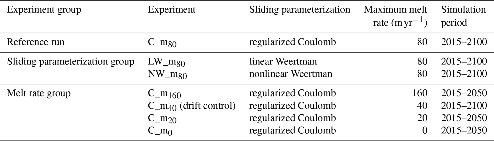
In this study, we conduct a series of simulations to assess the dynamic response of TG under different basal sliding parameterizations from the years 2015 to 2100 and sub-shelf melt rates from the years 2015 to 2050. We use the full-Stokes ice flow model, solved by Elmer/Ice (Gagliardini et al., 2013). Full-Stokes models consider all the components of the 3D deviatoric stress tensor. Furthermore, full-Stokes models have been suggested as essential for inferring a correct pattern of basal drag and for capturing all higher-order stresses near the grounding line of ice streams (Morlighem et al., 2010). Therefore, we expect to gain more insight into basal processes using a full-Stokes model. We specify three types of basal sliding parameterizations (linear and nonlinear Weertman and regularized Coulomb) and a range of sub-shelf melt rates with the same parameterization but different maximal basal melt rates of 0, 20, 40, 80, and 160 m yr⁻¹. We compare the results from the different simulations and investigate the impact of different basal sliding parameterizations and sub-shelf melt rates on TG evolution.

2 Data, model domain, and mesh refinement

2.1 Data

The Totten subregion is part of the Aurora Basin of the EAIS. We take its 2D domain boundary outline and ice front location from the MEaSUREs Antarctic Boundaries for IPY 2007–2009 from Satellite Radar version 2 dataset (Mouginot et al., 2017). The bed elevation, surface elevation (Fig. 1), and ice thickness are derived from MEaSUREs BedMachine Antarctica version 2 at a resolution of 500 m (Morlighem et al., 2020). The surface ice velocity data (Fig. 1), with a resolution of 450 m, are obtained from the MEaSUREs InSAR-based Antarctic ice velocity Map version 2 (Rignot et al., 2017).

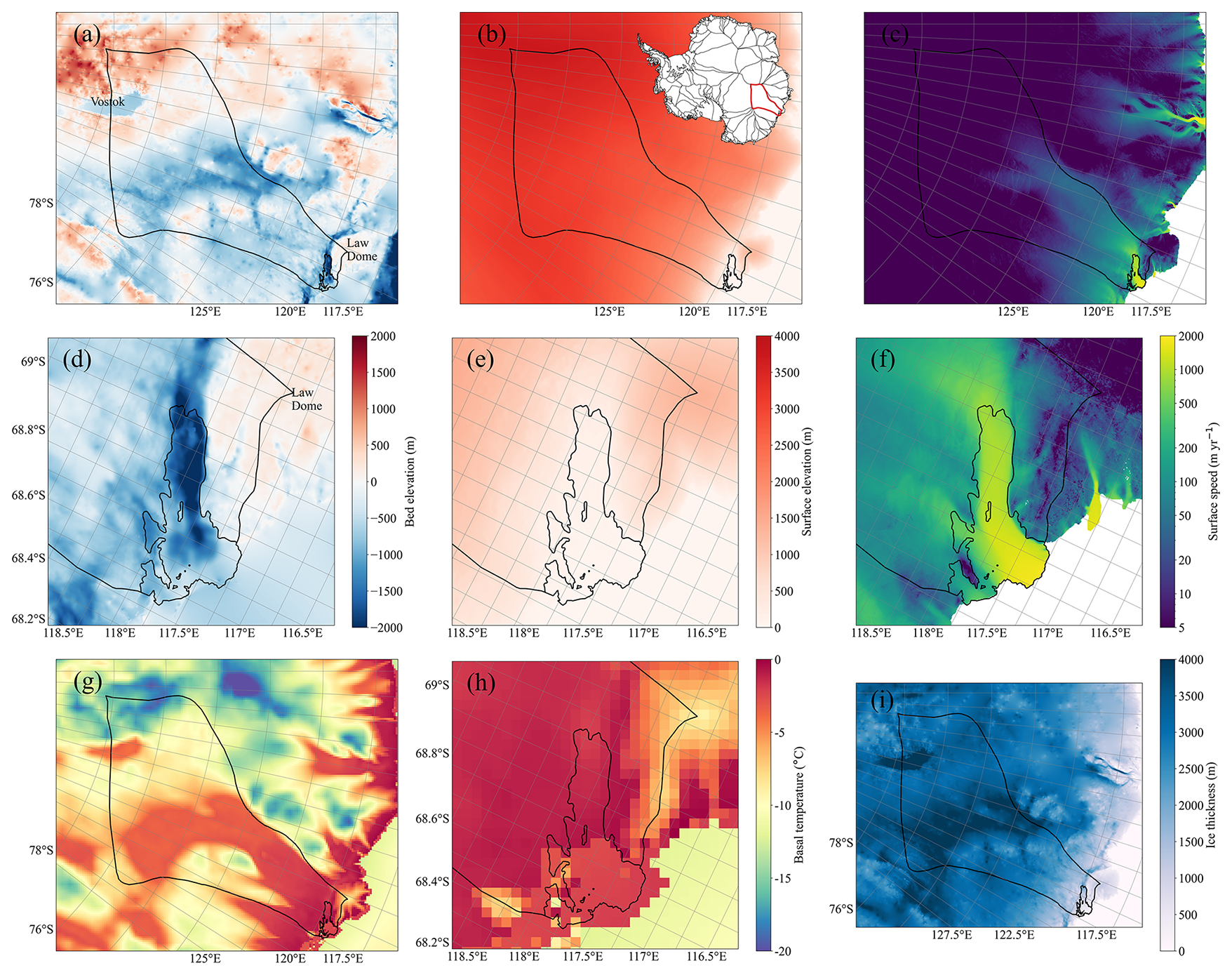
Figure 1 Bed elevation (a), surface elevation (b), surface ice flow speed (c), modelled basal temperature (g), and ice thickness (i) of the Totten subregion and its surroundings. The solid black curve is the outline of the Totten subregion, from the MEaSUREs Antarctic Boundaries for IPY 2007–2009 from Satellite Radar version 2 dataset (Mouginot et al., 2017). The inland black curve is the grounding line. The bed and surface elevations are from MEaSUREs BedMachine Antarctica version 2 (Morlighem et al., 2020). The surface ice flow speed is from the MEaSUREs InSAR-based Antarctic ice velocity Map version 2 (Rignot et al., 2017). The subglacial Lake Vostok and Law Dome are marked in plot (a). The inset plot in plot (b) shows drainage basin divisions and the location of our domain (red curve) in Antarctica. The prescribed ice temperatures are taken from the output of the ice sheet model SICOPOLIS (Greve et al., 2020). Panels (d)–(f) show the enlarged coastal region of (a)–(c), and (h) shows the enlarged coastal region of (g).

Ice sheet temperature data, at 8 km resolution (Fig. 1d), are sourced from the output files of the ice sheet model SICOPOLIS (Greve et al., 2020), which is initialized by a palaeoclimatic spin-up over 140 000 years until 1990, when the topography is nudged towards that of the present day (Greve et al., 2020). The geothermal heat flux applied in the study of Greve et al. (2020) is from Martos et al. (2017), at a resolution of 15 km. The surface mass balance (SMB) data applied for the period 2015–2100 consist of repeated 1995–2030 time-varying output of the Community Earth System Model version 2 (CESM2) of the Coupled Model Intercomparison Project Phase 6 (CMIP6) under the SSP5-8.5 scenario at 32 km resolution (Nowicki et al., 2016; Fig. S1 in the Supplement), which is close to the RACMO2.4p1 SMB data (Van Dalum et al., 2024). The ocean forcing is simplified to a parameterization scheme based on the Whole Antarctic Ocean Model (WAOM v1.0) output for modelling the basal melt rate of the ice shelves (see Sect. 3.3). See Table 1 for the dataset details.

Table 1 Datasets used in this study.

2.2 Mesh generation and refinement

We use Gmsh software (Geuzaine and Remacle, 2009) to generate an initial 2D horizontal footprint mesh within the domain boundary. The initial grid was then optimized by the anisotropic mesh adaptation code Mmg (Dapogny et al., 2014), which helps to refine the mesh where ice velocity and thickness gradients identify regions needing increased resolution. The resulting mesh is shown in Fig. 2 and has minimum and maximum element sizes of approximately 900 m and 20 km. The 2D mesh contains 31 434 elements and 15 996 nodes. It is then vertically extruded using 20 terrain-following layers, with a vertically refined mesh toward the base.

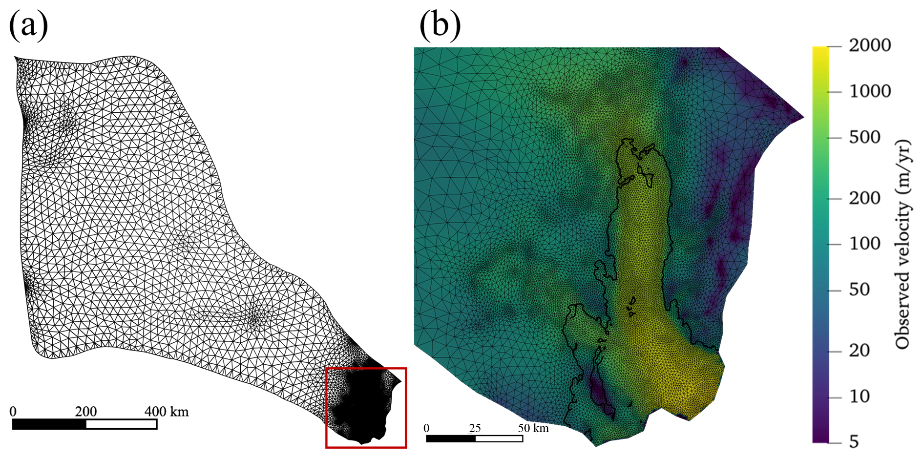
Figure 2 The refined 2D horizontal domain footprint mesh (a). The box outlined in panel (a) is shown in detail and overlain with surface ice velocity in panel (b). The solid black curves in (b) represent the positions of the grounding line.

3 Method

3.1 Ice flow model

We carried out all the simulations using the Elmer/Ice version 9.0 ice flow model (Gagliardini et al., 2013). We solve the Stokes equation and use a variational inverse method (Morlighem et al., 2010) as implemented in Elmer/Ice (Gagliardini et al., 2013; Gillet-Chaulet et al., 2012) to determine the basal friction coefficient in the linear Weertman sliding parameterization and a stress enhancement factor. The Stokes equation includes conservation equations for the momentum and mass:

$$\begin{array}{}\text{(1)}& {\displaystyle }\mathrm{\nabla }\cdot \mathit{\tau }-\mathrm{\nabla }p={\mathit{\rho }}_{\mathrm{i}}\mathit{g},\text{(2)}& {\displaystyle }\mathrm{\nabla }\cdot \mathit{v}=\mathrm{0},\end{array}$$

where τ is the deviatoric stress tensor, p is the isotropic pressure, ρ_i is the ice density, g is the acceleration due to gravity (0, 0, −9.81 m s⁻²), and v is ice velocity. The effective viscosity, η, or the ice rheology,

$$\begin{array}{}\text{(3)}& \mathit{\tau }=\mathrm{2}\mathit{\eta }\dot{\mathit{\epsilon }},\end{array}$$

given by Glen's flow law (Cuffey and Paterson, 2010),

$$\begin{array}{}\text{(4)}& \mathit{\eta }={\displaystyle \frac{\mathrm{1}}{\mathrm{2}}}(E\cdot A(T){)}^{-\frac{\mathrm{1}}{n}}{\dot{\mathit{\epsilon }}}_{\mathrm{e}}^{\frac{\mathrm{1}-n}{n}},\end{array}$$

is dependent on ice temperature via the flow rate factor A(T), defined by an Arrhenius equation. We use an exponent of n=3. $\dot{\mathit{\epsilon }}$ denotes the strain rate, and the term ${\dot{\mathit{\epsilon }}}_{\mathrm{e}}=\sqrt{\text{tr}\left({\dot{\mathit{\epsilon }}}^{\mathrm{2}}\right)/\mathrm{2}}$ is the effective strain rate. The ice temperature distribution comes from the output of the ice sheet model SICOPOLIS (Greve et al., 2020). We introduce $E_{\mathit{\eta }}=E^{-\mathrm{1}/\left(\mathrm{2}n\right)}$ to obtain

$$\begin{array}{}\text{(5)}& \mathit{\eta }={\displaystyle \frac{\mathrm{1}}{\mathrm{2}}}{E}_{\mathit{\eta }}^{\mathrm{2}}\cdot A(T{)}^{-\frac{\mathrm{1}}{n}}{\dot{\mathit{\epsilon }}}_{\mathrm{e}}^{\frac{\mathrm{1}-n}{n}},\end{array}$$

which ensures η>0 for any value of E_η. We refer to E_η as the 2D vertically constant stress enhancement factor, which is set initially to unity everywhere, indicating no stress enhancement, before performing the viscosity inversion. The enhancement factor is often used to account for anisotropy effects (Ma et al., 2010). Values of E_η<1 indicate softer and faster-deforming ice, whereas higher values, E_η>1, mean stiffer ice.

The ice surface is assumed to have a vanishing Cauchy stress vector. At the ice front below sea level and the bottom of the ice shelf, the normal Cauchy stress is set equal to the hydrostatic water pressure. The so-called sea spring (Gagliardini et al., 2013) stabilization method is applied to the bottom free surface in the case of a temporal evolution away from the hydrostatic equilibrium. On the lateral boundary, the normal stress is equal to the hydrostatic ice pressure, and the normal velocity is set to zero, while the ice is free to slip in the tangential direction. The bed for grounded ice is assumed to be rigid, impenetrable, and fixed over time since the ice sheet geometry change over decades is too small to affect lithosphere deformation (de Boer et al., 2014; Coulon et al., 2021). The normal component of the velocity is set to zero at the ice–bed interface. We implement alternative basal sliding relations (Sect. 3.2) for the grounded ice in Elmer/Ice. For transient simulations, we prescribe SMB at the ice surface (Sect. 2.1) and sub-shelf basal melt rate parameterization along the surface in contact with the ocean (Sect. 3.3).

3.2 Basal sliding parameterizations and conversion between them

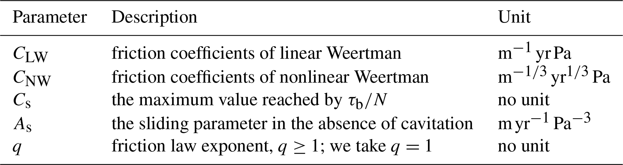
We use three basal sliding parameterizations in this study: linear Weertman sliding (Eq. 6), nonlinear Weertman sliding (Eq. 7; Weertman, 1957), and regularized Coulomb sliding parameterization (Eqs. 8 and 9; Schoof, 2005; Gagliardini et al., 2007) given by

$$\begin{array}{}\text{(6)}& {\displaystyle }{\mathit{\tau }}_{\mathrm{b}}=C_{\text{LW}}{\mathit{u}}_{\mathrm{b}},\text{(7)}& {\displaystyle }{\mathit{\tau }}_{\mathrm{b}}=C_{\text{NW}}{\mathit{u}}_{\mathrm{b}}^{\mathrm{1}/m},\text{(8)}& {\displaystyle }{\mathit{\tau }}_{\mathrm{b}}=C_{\mathrm{s}}N{\left[{\displaystyle \frac{\mathit{\chi }\cdot u_{\mathrm{b}}^{-m}}{\mathrm{1}+a\cdot {\mathit{\chi }}^q}}\right]}^{\frac{\mathrm{1}}{m}}{\mathit{u}}_{\mathrm{b}},\text{(9)}& {\displaystyle }\mathit{\chi }={\displaystyle \frac{u_{\mathrm{b}}}{C_{\mathrm{s}}^m{N}^m{A}_{\mathrm{s}}}},\end{array}$$

where τ_b is the basal shear stress, u_b is the vector of the basal sliding velocity, u_b is the basal sliding speed, and C_LW and C_NW are friction coefficients of the linear and nonlinear Weertman sliding parameterizations. We set m=3. The regularized Coulomb sliding parameterization considers the existence of water cavities which may be present between ice and soft sediment layers. The parameter A_s is the sliding parameter in the absence of cavitation, and C_s is the maximum value reached by ${\mathit{\tau }}_{\mathrm{b}}/N$ (Gagliardini et al., 2007). In Eq. (8), q is a post-peak exponent satisfying q≥1; $a=(q-\mathrm{1}{)}^{q-\mathrm{1}}/q^q$. We assume q=1, obtaining a=1. N represents the effective pressure on the ice bottom and is defined as $N={\mathit{\sigma }}_{\text{nn}}-p_{\mathrm{w}}$, where σ_nn is the normal stress at the bed, and p_w is the water pressure. The parameters and their units are listed in Table 2.

Table 2 List of parameters used in Sect. 3.2 and their units.

Lower effective pressure reduces the basal friction and enhances the basal sliding speed. This effect has been included in several sliding parameterizations (Budd et al., 1984; Schoof, 2005; Tsai et al., 2015). Hydrology models determining the effective pressure distribution rely on a set of poorly constrained parameters, such as sheet and channel conductivities and basal melt water input, which are hard to measure (Werder et al., 2013). Therefore, many authors take effective pressure as the hydrostatic pressure imposed by an assumed perfect connection between the subglacial drainage system and the ocean (Morlighem et al., 2010; Tsai et al., 2015; Gladstone et al., 2017). For TG, Dow et al. (2020) simulated the basal hydrology using the GlaDS subglacial hydrology model to best match the specularity content and found the modelled water pressure is ∼95 % of overburden in most of the region. Motivated by their findings, in this study, we take the effective pressure as 5 % of overburden. This assumption decreases the effective pressure by an order of magnitude in most inland regions and halves it near the GL, compared with that under the assumption of perfect hydrostatic connection (Fig. S2 in the Supplement).

We apply the basal shear stress and basal sliding velocity field obtained from the inversion with the linear Weertman sliding parameterization to the other two sliding parameterizations and estimate the sliding parameters there. In other words, we convert the local friction coefficient in the linear Weertman sliding parameterization to that in other sliding parameterizations (Brondex et al., 2017). In Eq. (6), we set C_LW=10^β to make sure C_LW is positive. The conversion from C_LW to C_NW is then trivially given by $C_{\text{NW}}={\mathrm{10}}^{\mathit{\beta }}{u}_{\mathrm{b}}^{\mathrm{1}-\mathrm{1}/m}$. To convert the friction coefficient from a linear Weertman to a regularized Coulomb sliding parameterization, as given in Eq. (8), we rearrange the latter:

$$\begin{array}{}\text{(10)}& {\left({\displaystyle \frac{{\mathit{\tau }}_{\mathrm{b}}}{C_{\mathrm{s}}N}}\right)}^m={\displaystyle \frac{\mathit{\chi }}{\mathrm{1}+\mathit{\chi }}}.\end{array}$$

The limit forms of Eq. (10) with small χ→0 or large χ>10 correspond to slow-flowing regimes with large effective pressure and fast-flowing regimes with small effective pressure, respectively.

In the limit of small χ, we recover a nonlinear Weertman law:

$$\begin{array}{}\text{(11)}& {\mathit{\tau }}_{\mathrm{b}}=A_{\mathrm{S}}^{-\mathrm{1}/m}{u}_{\mathrm{b}}^{\mathrm{1}/m}.\end{array}$$

Combining Eqs. (11) and (6) with C_LW=10^β, we get

$$\begin{array}{}\text{(12)}& A_{\mathrm{s}}=({\mathrm{10}}^{\mathit{\beta }}\cdot u_{\mathrm{b}}^{\mathrm{1}-\mathrm{1}/m}{)}^{-m}.\end{array}$$

In the limit of Eq. (10) for large χ (i.e. N is relatively small), we obtain a Coulomb type of friction:

$$\begin{array}{}\text{(13)}& {\mathit{\tau }}_{\mathrm{b}}=C_{\mathrm{s}}N.\end{array}$$

We modify Eq. (12) by multiplying a smooth transition term from a small-N region to a large-N region as below such that it can be applied to the whole region:

$$\begin{array}{}\text{(14)}& A_{\mathrm{s}}=\tanh \left(\mathrm{2}N\right)\cdot ({\mathrm{10}}^{\mathit{\beta }}\cdot u_{\mathrm{b}}^{\mathrm{1}-\mathrm{1}/m}{)}^{-m}.\end{array}$$

Combining Eqs. (6), (8), and (9) with C_LW=10^β, then using Eq. (14), we can get C_s in the regularized Coulomb sliding parameterization as

$$\begin{array}{}\text{(15)}& \begin{array}{rl}{C}_{\mathrm{s}}& ={\displaystyle \frac{{\mathrm{10}}^{\mathit{\beta }}\cdot u_{\mathrm{b}}}{N\cdot (\mathrm{1}-{\mathrm{10}}^{m\mathit{\beta }}\cdot A_{\mathrm{s}}\cdot u_{\mathrm{b}}^{m-\mathrm{1}}{)}^{\mathrm{1}/m}}}\\ & ={\displaystyle \frac{{\mathrm{10}}^{\mathit{\beta }}\cdot u_{\mathrm{b}}}{N\cdot (\mathrm{1}-\tanh (\mathrm{2}N){)}^{\mathrm{1}/m}}}.\end{array}\end{array}$$

Equations (14) and (15) determine the conversion of the inverted friction coefficients to the regularized Coulomb sliding parameterization. We keep the converted friction coefficients A_s and C_s fixed in all the prognostic simulations with the regularized Coulomb sliding parameterization.

Equation (10) is equivalent to Coulomb-type friction with a factor

$$\begin{array}{}\text{(16)}& {\mathit{\tau }}_{\mathrm{b}}={\left({\displaystyle \frac{\mathit{\chi }}{\mathrm{1}+\mathit{\chi }}}\right)}^{\mathrm{1}/m}{C}_{S}N.\end{array}$$

This factor $(\frac{\mathit{\chi }}{\mathrm{1}+\mathit{\chi }}{)}^{\mathrm{1}/m}$ is about 0.6 if χ=0.275, about 0.8 if χ=1, and about 0.97 if χ=10.

3.3 Ice shelf basal melt parameterization

Sub-shelf melting of TG is influenced by ocean heat intrusions imposed by mCDW, which may be modified by several processes, such as the Antarctic Slope Current and upstream coastal freshening (Nakayama et al., 2021). But we do not consider the complex ocean circulation here. Instead, we use a simplified parameterization to mimic the spatial pattern and magnitude inferred from satellites (Rignot et al., 2013; Depoorter et al., 2013; Liu et al., 2015; Adusumilli et al., 2020) and ocean model simulations (Richter et al., 2022). We consider sub-shelf melt as the sum of low melt, which plays a dominant role in the shallow water (<500 m), and high melt, which plays a dominant role in the deep water (>1000 m) near the grounding line. We express mass balance in ice equivalent units.

We parameterize the sub-shelf melt rate in the shallow water using ice shelf bottom depth and ice shelf basal melting rate as modelled by the 2 km spatial resolution, tide, and eddy-resolving Whole Antarctic Ocean Model (WAOM v1.0; Richter et al., 2022). We performed linear regression between the sub-shelf melt rate and $\mathrm{1}/(d+d_{\mathrm{0}})$, where d is the ice shelf bottom depth (unit: m), and d₀ is a tuned parameter. We found the best fit as follows with d₀=100 m (Fig. S3 in the Supplement):

$$\begin{array}{}\text{(17)}& M_{\mathrm{d}}=\mathrm{450.284}\times {\displaystyle \frac{\mathrm{1}}{d+d_{\mathrm{0}}}}+\mathrm{1.1917},\end{array}$$

where M_d represents the basal melting rate of the ice shelf (unit: m yr⁻¹).

The WAOM v1.0 estimates of Antarctic ice shelf basal mass loss agree with satellite observations in many regions (Richter et al., 2022). However, for the TG subregion, the satellite estimates (Rignot et al., 2013; Depoorter et al., 2013; Liu et al., 2015; Adusumilli et al., 2020) suggest higher basal melting (area average melt ≥10 m yr⁻¹) than that obtained with WAOM v1.0 (Richter et al., 2022). To account for the high melt rate in the deep water, we add an extra melt rate term as

$$\begin{array}{}\text{(18)}& M_{\mathrm{e}}=\left\{\begin{array}{ll}{M}_{max}\times \left(\frac{d}{\mathrm{2000}}\right),& d<\mathrm{2000}\mathrm{m};\\ M_{max},& d\ge \mathrm{2000}\mathrm{m},\end{array}\right.\end{array}$$

where M_max is the maximum basal melt rate, and d is the depth of the bottom surface of the ice shelf (unit: m).

In addition, we use two scaling factors, S_w and S_i, to reflect the influence of cavity geometry and avoid numerical instability caused by a vanishingly thin ice shelf, following Gladstone et al. (2017):

$$\begin{array}{}\text{(19)}& S_{\mathrm{w}}=\tanh \left(e{\displaystyle \frac{H_{\mathrm{w}}}{H_{\text{w0}}}}\right),\end{array}$$

where H_w is the water column thickness, given by $H_{\mathrm{w}}=z_{\mathrm{i}}-b$, where z_i is the ice shelf bottom elevation and b is the bed elevation. We set H_w0=200 m as a reference water column thickness. S_w approaches 1 with a thick water column (H_w>H_w0), and S_w approaches 0 when the water column thickness goes to 0 near the grounding line, capturing the influence of cavity geometry on melt rate as a very thin water column restricts circulation. A high step change in forcing across the grounding line (basal drag or ocean-induced melt) causes problems for stability (Gladstone et al., 2017). S_w prevents high melting right next to the grounding line, thus reducing that step change.

A vanishingly thin ice shelf causes the tetrahedral elements to have a very high horizontal to vertical length scale, which increases the likelihood of instability. S_i is an ice shelf depth-scaling parameter, used to prevent melting of the ice shelf once the draft passes $\left|z_{\text{i0}}\right|$, given by

$$\begin{array}{}\text{(20)}& S_{\mathrm{i}}=max\left[\tanh \left(e{\displaystyle \frac{z_{\text{i0}}-z_{\mathrm{i}}}{z_{\mathrm{s}}}}\right),\mathrm{0}\right],\end{array}$$

where we set $z_{\text{i0}}=-\mathrm{80}$ m as a reference ice base elevation relative to sea level (positive upwards) and z_S=100 m as a (directionless) scaling depth. The use of S_i gives zero melting for z_i>z_i0.

Combining Eqs. (17)–(20), the sub-shelf melt rate is then parameterized as

$$\begin{array}{}\text{(21)}& M=S_{\mathrm{w}}\cdot S_{\mathrm{i}}\left(M_{\mathrm{d}}+M_{\mathrm{e}}\right).\end{array}$$

The parameterizations of M_d and M_e with M_max=40 m yr⁻¹ and the total sub-shelf melt with water column thickness along a flowline are illustrated in Fig. S3. The spatial distributions of estimated sub-shelf melt rates using different values of M_max (0, 20, 40, 80, and 160 m yr⁻¹) are shown in Fig. 3. The modelled sub-shelf melt rates, with varying maximal values, cover most of the estimates from previous studies.

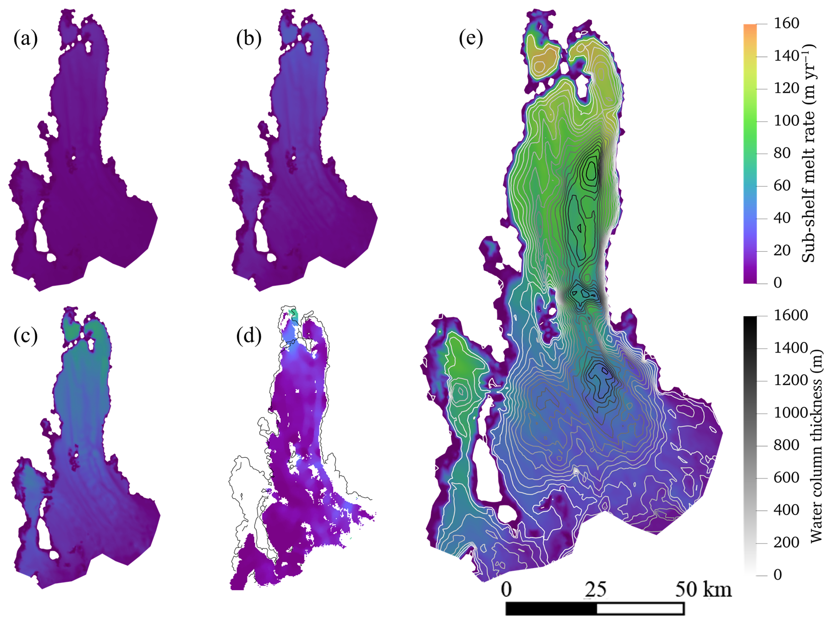
Figure 3 Spatial distribution of modelled sub-shelf melt rate with maximum values of (a) 20, (b) 40, (c) 80, and (e) 160 m yr⁻¹, with coloured contours indicating water column thickness under the ice shelf with 100 m intervals. Plot (d) shows the satellite-based estimates (Adusumilli et al., 2020).

Flux gate calculations using satellite data have reported steady-state area-averaged basal melt rates of 10.5 ± 0.7 m yr⁻¹ (2003–2008; Rignot et al., 2013), 9.89 ± 1.92 m yr⁻¹ (2003–2009; Depoorter et al., 2013), and 11.5 ± 2.0 m yr⁻¹ (2010–2018; Adusumilli et al., 2020). Notably, Liu et al. (2015) used a similar method without assuming a steady-state calving front and derived a higher melt rate of 17.9 ± 1.2 m yr⁻¹ during the period 2003–2011. This elevated value aligns better with Rintoul et al.'s (2016) synoptic cavity water exchange estimates. In situ measurements by Vaňková et al. (2023), using autonomous phase-sensitive radar along grounding lines, revealed large spatial melt variability, correlating with water column thickness gradients. Our model simulations for sub-shelf melt rate with maximum values of 20, 40, 80, and 160 m yr⁻¹ (Fig. 3) yield area-averaged melt rates of 7.8, 14.0, 26.6, and 51.6 m yr⁻¹, respectively, for the present-day ice shelf geometry.

3.4 Experiment design

The following simulations are carried out in series as part of the initialization procedure. We first do a steady-state simulation with E_η=1 and the linear Weertman sliding parameterization, expressing the sliding coefficient as C_LW=10^β, where β is from the output of a whole Antarctic Ice Sheet inversion for the year 2015 (Gladstone et al., 2019) and linearly interpolated from that mesh to the finer mesh in this study. We then relax the free surface of the domain by a short transient run of 1 year with a small time-step size of 0.1 year without any sub-shelf melt rate to reduce the non-physical spikes in the initial surface geometry (Zhao et al., 2018; Wang et al., 2022). Taking the results from surface relaxation, we use the variational inverse method (Morlighem et al., 2010) to adjust the spatial distribution of the basal friction coefficient and stress enhancement factor to minimize the mismatch between the magnitudes of the simulated and observed (Fig. 1c; Table 1) surface velocities, following the same approach as in Gladstone and Wang (2022) and Wang et al. (2022). The inversions make use of Tikhonov regularization (Gillet-Chaulet et al., 2012). Two separate regularization parameters, λ_β and λ_η, are used for the drag inversions and stress enhancement factor inversions. The total cost function, J_tot, is the sum of the misfit, J₀, and weighted regularization term for the drag inversion:

$$\begin{array}{}\text{(22)}& J_{\text{tot}}=J_{\mathrm{0}}+{\mathit{\lambda }}_{\mathit{\beta }}{J}_{\text{reg}}.\end{array}$$

λ_β would be replaced by λ_η for the viscosity enhancement factor inversion. We take λ_β=10³ and λ_η=10⁴. We first obtain the optimal spatial field of β, an updated modelled ice velocity field, and the stress field. We then perform a viscosity inversion to obtain the optimal spatial field of E_η and further updated modelled ice velocity and stress fields. We take this state as the one for the initial year 2015.

With the modelled basal shear stress and basal sliding velocity, we convert the basal drag coefficient from the linear Weertman parameterization to the basal drag coefficients representing nonlinear Weertman and regularized Coulomb parameterizations using the method described in Sect. 3.2. Using the three different sliding parameterizations and different sub-shelf melt rates, we carry out two sets of sensitivity tests (Table 3). We run simulations in the sliding parameterization group from 2015 to 2100 and melt rate group from 2015 to 2050, all with a time-step size of 0.1 years. A so-called “reference run” is chosen to illustrate a more dynamic process during the 85-year simulation. We chose regularized Coulomb parameterization as the basal sliding in the reference run because it is arguably the most physically sound (Tsai et al., 2015; Joughin et al., 2019). Given the expectation of a warming climate, we chose for our reference run a melt rate parameterization with a maximum melt that approximates to an estimate for the temporal maximum over recent decades (i.e. 80 m yr⁻¹; Adusumilli et al., 2020; Nakayama et al., 2021). We use maximum sub-shelf melt rates of 0, 20, 40, 80, and 160 m yr⁻¹ (Fig. 3) in the sensitivity tests. We did simulations of the melt rate group to the year 2050 because solving the Stokes equation for the Totten Glacier subregion is computationally expensive, and the sensitivity of Totten Glacier dynamics to the sub-shelf melt rate has been shown from 2015 to 2050. Since the modelled sub-shelf melt rate with the maximum value of 40 m yr⁻¹ is closest to the satellite-based estimates (Sect. 3.3), the experiment C_m₄₀ (which belongs to the melt rate group) was selected as the control experiment to evaluate the model drift and was done from 2015 to 2100. In the drift control experiment C_m₄₀, the modelled annual mean thinning rate from 2015 to 2020 is −0.03 m yr⁻¹, which is larger than the observed thinning rate of −0.02 m yr⁻¹ (Nilsson et al., 2023), indicating higher model sensitivity to the present-day climate forcing.

Table 3 Summary of sensitivity experiments.

4 Results

4.1 Initial state and reference run result

We obtain the inverted optimal spatial distribution of the basal sliding coefficient exponent β (Fig. 4a) in the linear Weertman parameterization and the stress enhancement factor (Fig. 4b) for the initial year 2015 and keep them fixed in all the prognostic simulations. The basal sliding coefficient exponent β is smaller in the fast-flow regions where ice speed >10 m yr⁻¹ and larger in the slow-ice-flow region. The inversion results show a rib-like pattern of the basal sliding coefficient and basal shear stress in the fast-flowing region (Fig. 4e and g). But it does not directly give us the cause. Ripples, oscillations, and ribs have been found in other inverse models of both Greenland and Antarctica (Sergienko and Hindmarsh, 2013; Sergienko et al., 2014; Wolovick et al., 2023). E_η remains at 1 over most of the grounded region; E_η>1 in the vicinity of the grounding line indicates relatively stiffer ice; and E_η<1 on the ice shelf indicates more rapid deformation, likely due to shear-band damage.

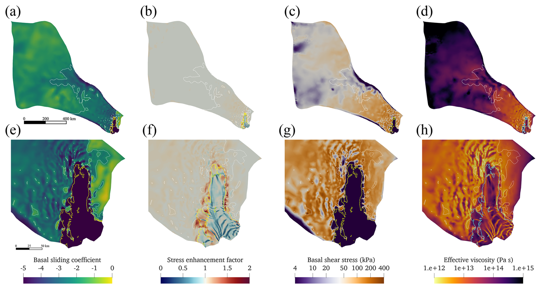
Figure 4 Spatial distribution of the modelled (a) basal sliding coefficient β, (b) stress enhancement factor E_η, (c) basal shear stress, (d) basal effective viscosity, and their corresponding enlarged details (e–h). The solid yellow (a–c, e–g) and cyan (d, h) curves represent the grounding line, and the solid white curves in (a)–(d) show modelled basal speed contours of 10 m yr⁻¹.

The converted friction coefficients A_s and C_s in the regularized Coulomb sliding parameterization are also kept fixed in the prognostic simulations. The value of χ (Eq. 9) in the initial year is from 0.3 to 0.5 near the grounding line with spatial variability, mainly on the eastern branch, which means that the basal friction in the fast-flowing region is 60 %–70 % of that in a true Coulomb regime (Eq. 16). As the effective pressure is reduced as the ice thins, χ increases and varies from 0.3 to 5 near the grounding line in the year 2100, which is closer to a true regularized Coulomb sliding parameterization (Fig. S4 in the Supplement).

For the initial year 2015, the basal shear stress (Fig. 4c) for the initial state is concentrated in the range of 4–400 kPa. The basal effective viscosity (Fig. 4d) is smaller in regions with relatively high ice temperature (Fig. 1) and fast flow speed (>10 m yr⁻¹) and larger in the upstream regions with low ice temperature and slow flow speed. Shear margins of lower viscosity exist on both sides of the TIS.

In the reference run (C_m₈₀), ice thickness upstream of the grounding line decreases notably, and the ice velocity speeds up upstream of the grounding line but decelerates near the ice front of the ice shelf over the 85-year simulation (Fig. 5). But there are large spatial differences in ice thickness change in the grounded ice. The fast-flowing regime in the grounded ice becomes larger, and the ice shows dynamic thinning at the eastern and southern grounding line (Fig. 5). The western side of TIS is grounded on Law Dome (Fig. 1). The grounding line retreats primarily along the southern and eastern grounding zones, which is consistent with previous studies (e.g. Pelle et al., 2021). We select two flowlines for analysis: FL1 along the main trunk and FL2 on the eastern branch (Fig. 5) of TG. The modelled annually averaged grounded ice thinning rate from 2015 to 2100, measured from the 2100 grounding line position and extending 20 km further upstream, is 2.14–2.35 m yr⁻¹ along FL1 and 2.88–5.06 m yr⁻¹ along FL2. The modelled grounding line retreats 12.20 km along FL1 and 23.29 km along FL2 by the year 2100. The basal topography along FL1 is a prograde-sloping bed with a large slope upstream of the grounding line, but the basal topography along FL2 has more variations in slope, and the slopes are smaller than those along FL1. Hence, the ice is more stable along FL1 than along FL2.

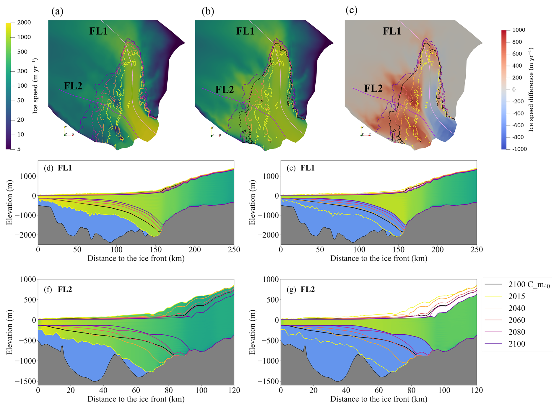
Figure 5 Surface velocity at the beginning of the initial year 2015 (a) and the end of the year 2100 (b) in the reference run. The surface velocity difference (2100 minus 2015) is shown in (c). The grounding line positions in the years 2015, 2040, 2060, 2080, and 2100 in the reference run C_m₈₀ are shown in (a)–(c). The grounding line position in the year 2100 in the drift control run C_m₄₀ is shown in (b)–(g) with black lines. The solid pink and purple lines in (a) and (b) represent flowlines FL1 and FL2 as labelled. The solid colour portions of the figures show the ice flow velocity (upper colour bar) profiles along FL1 (d, e) and FL2 (f, g) in the reference run in the initial year 2015 (d, f) and the end year 2050 (e, g), with bedrock in dark grey and seawater in blue. The geometry change in TG is marked with solid coloured lines for the years 2015, 2040, 2060, 2080, and 2100. The vertical elevations are exaggerated by a factor of 25.

4.2 Sensitivity experiment results

The grounding lines at the years 2050 and 2100 from the sliding parameterization and at the year 2050 from the melt rate groups are shown in Fig. 6. The grounding line mainly retreats in the southern and eastern grounding zones, and grounding line evolution is sensitive to both sliding parameterizations and sub-shelf melt rates (Fig. 6). The modelled grounding line retreats the most using the linear Weertman sliding parameterization, slightly less using the regularized Coulomb sliding parameterization, and the least using the nonlinear Weertman sliding parameterization (Fig. 6). The grounding line retreats more using the regularized Coulomb sliding parameterization than with the nonlinear Weertman sliding parameterization, which might be because the effective pressure used in the regularized Coulomb is reduced as the ice thins, leading to more basal sliding and faster ice speed. Moreover, the value of χ (Eq. 9) is below 1 in the fast-flowing region from our posterior estimate, showing a reduced basal friction and enhanced basal sliding (Eq. 16) compared with a true regularized Coulomb sliding parameterization.

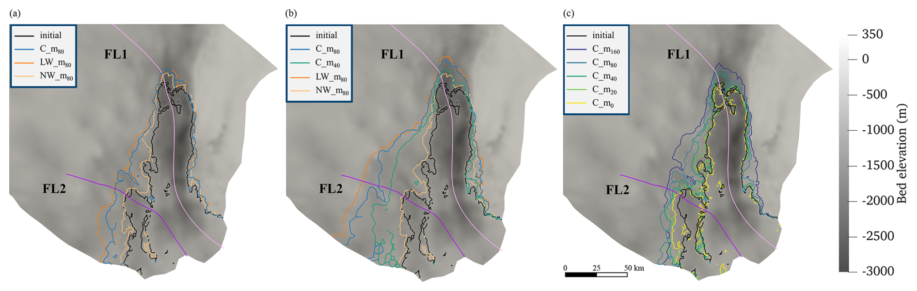
Figure 6 Grounding line positions (coloured curves) at the year 2050 from experiments in the sliding parameterization group (a), at the year 2100 from experiments in the sliding parameterization group and drift control experiment (b), and at the year 2050 from experiments in the melt rate group (c). The solid black line represents the initial grounding line position in the year 2015. The solid pink and purple lines are FL1 and FL2, respectively. The grey background shows the bed elevation.

Along the main trunk FL1, both the regularized Coulomb (C_m₈₀) and the linear Weertman (LW_m₈₀) sliding parameterizations produce comparable grounding line retreat rates of 0.14 km yr⁻¹ over 2015–2100 (Fig. 7). These rates correspond to retreats of 8.08 km by 2050 and 12.20 km by 2100. In contrast, with the nonlinear Weertman sliding, retreats are 5.94 km by 2050 along FL1, followed by stabilization (Fig. 6). Meanwhile, the drift control experiment (C_m₄₀) shows a grounding line retreat of 8.08 km along FL1 by 2100. Along FL2, the grounding line retreats 12.09 km by 2050 and 35.85 km by 2100 (∼0.42 km yr⁻¹) using linear Weertman, 10.83 km by 2050 and 23.29 km by 2100 (∼0.27 km yr⁻¹) using regularized Coulomb, and only 1.32 km by 2050 (∼0.04 km yr⁻¹) followed by near stabilization using nonlinear Weertman sliding parameterizations (Fig. 6). Meanwhile, the drift control experiment (C_m₄₀) shows a grounding line retreat of 12.33 km along FL2 by 2100.

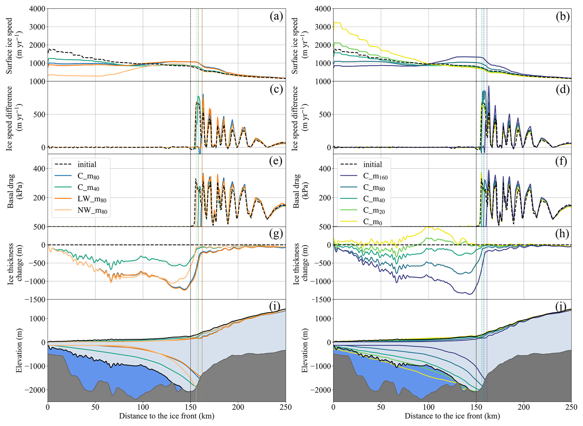
Figure 7 Surface ice speed (a, b), ice speed difference (c, d; surface minus basal), basal drag (e, f), ice thickness change (g, h), and ice sheet profiles (i, j) along FL1 in the initial year 2015 (solid black line) and the year 2100 (solid coloured line) from experiments (Table 3) in the sliding parameterization group and drift control experiment (a, c, e, g, i) and the year 2050 (solid coloured line) in the melt rate group (b, d, f, h, j). Grounding line positions are marked with the vertical dashed black line for the year 2015 and vertical dashed coloured line for the year 2100 in the sliding parameterization group (a, c, e, g, i) and the year 2050 (solid coloured line) in the melt rate group (b, d, f, h, j). The figure is shaded to show the geometry of the TG along the flowline in 2015, where dark grey is the bedrock, light blue is the ice shelf, and dark blue is seawater. The elevations are exaggerated by a factor of 25.

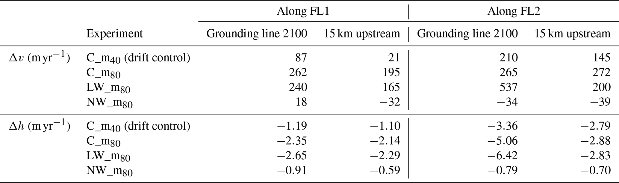
Between 2015 and 2100, when applying the regularized Coulomb and linear Weertman sliding parameterizations, the surface ice flow speed exhibits an acceleration upstream of the grounding line, and the ice thickness upstream of the grounding line experiences a gradual decrease. The ice flow speed acceleration and ice thinning are more pronounced in the eastern grounding zones compared to the southern ones (Figs. S5 and S6 in the Supplement). Conversely, when the nonlinear Weertman sliding parameterization is employed, the surface ice flow velocity undergoes a slight deceleration in the vicinity of the grounding line, while it experiences a slight acceleration at locations further upstream (Fig. S5). The surface lowering is much smaller using the nonlinear Weertman sliding parameterization than that using the regularized Coulomb and linear Weertman sliding parameterizations. The modelled grounded ice thinning rate in the reference run (C_m₈₀) near the projected 2100 grounding line is double that of the drift control run (C_m₄₀). Furthermore, surface ice velocity acceleration in C_m₈₀ at the projected 2100 grounding line position along the main trunk FL1 exceeds that in the drift control run by a factor of 3 over the 2015–2100 period (Table 4). More specifically, the surface ice speed change and ice thickness change along FL1 and FL2 from experiments in the sliding parameterization group and the drift control experiment are shown in Table 4 and Figs. 7 and 8.

Table 4 Surface ice speed change, Δv, and ice thickness change rate, Δh, from the years 2015 to 2100 (2100 minus 2015) at the projected 2100 grounding line position and 15 km further upstream, along FL1 and FL2 from the drift control experiment and experiments in the sliding parameterization group.

Figure 8 The same as Fig. 7 but for FL2.

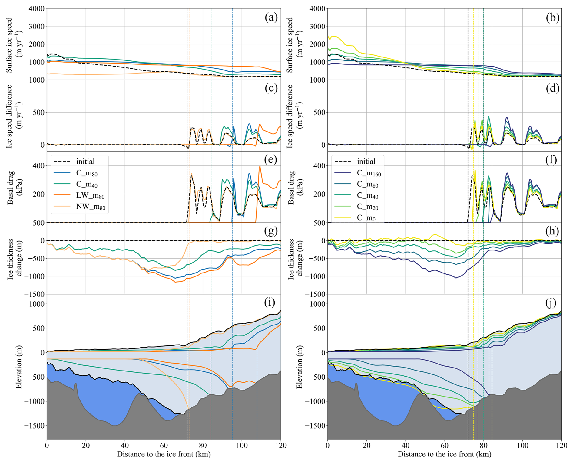
The oscillations in the difference between the surface and basal ice speeds near the grounding line and upstream are caused by the rib-like pattern of basal friction and basal velocity. The difference between surface and basal speeds drops to zero, which means the basal friction approaches zero in the fast-flowing trunks upstream of the grounding line (Figs. 7 and 8). The fast-flowing ice streams are supported by shear margins or isolated sticky regions through long-distance stress transmission (Wolovick et al., 2023).

The simulation grounded area loss rates between 2015 and 2100 from the sliding parameterization group experiments are heterogeneous in both time and space (Figs. 5, 6, and 9a). The grounded area loss is 3149, 2611, and 1105 km² by the year 2050 and 6582, 5601, and 1360 km² by the year 2100 with linear Weertman (LW_m₈₀), regularized Coulomb (C_m₈₀), and nonlinear Weertman (NW_m₈₀) sliding parameterizations, respectively (Fig. 9a). The grounded area losses in the LW_m₈₀ and C_m₈₀ experiments by 2100 significantly exceed the 3413 km² from the drift control experiment. The modelled grounded area loss using nonlinear Weertman after the year 2050 is much less than that before 2050. The modelled grounded area loss rate using regularized Coulomb (C_m₈₀) becomes slower from 2050 to 2075, while the glacier retreats over rumpled terrain and re-accelerates after the year 2075. The modelled grounded area using linear Weertman decreases at a nearly constant rate, becoming gradually slower in the last 2 decades.

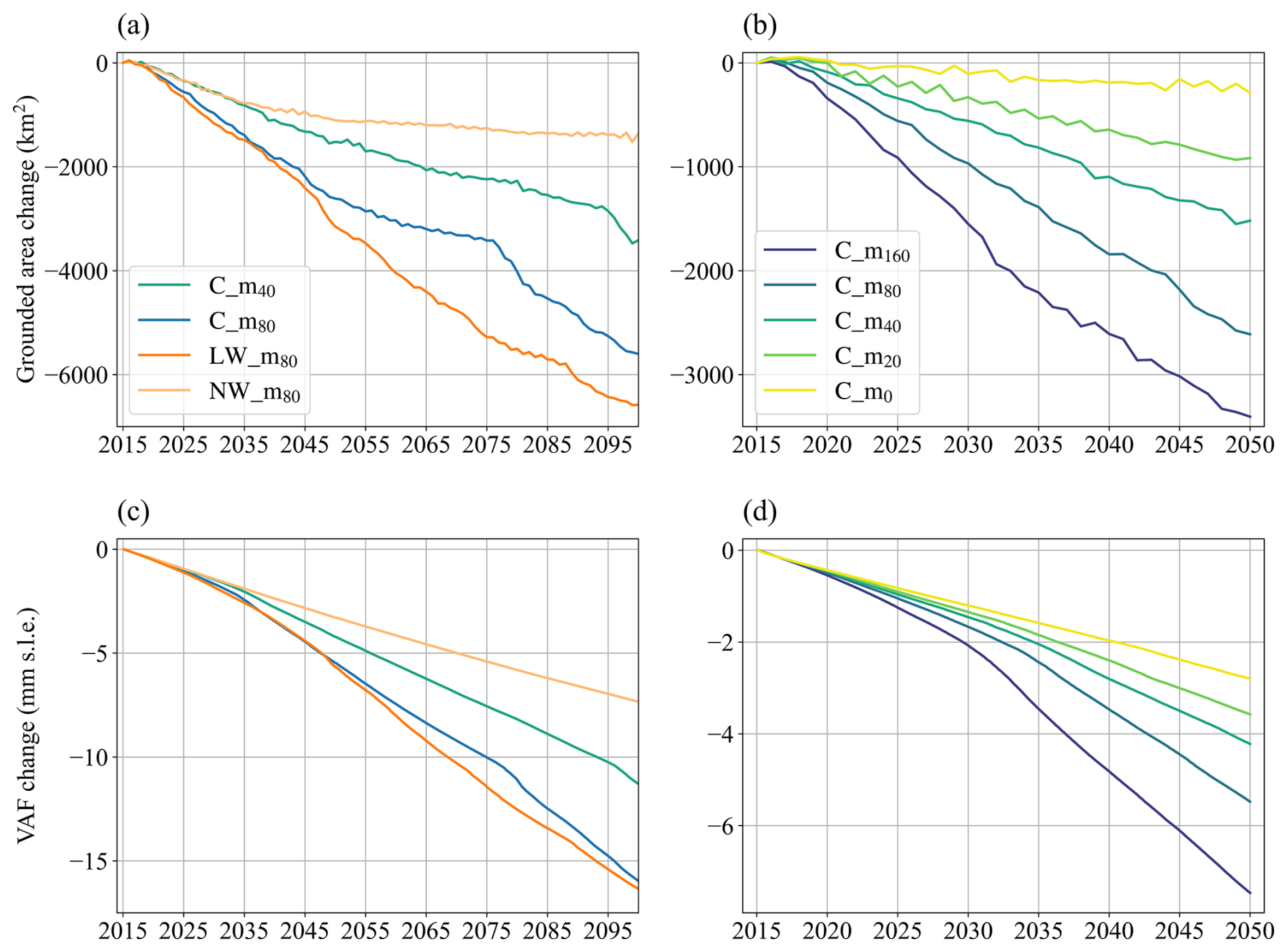
Figure 9 Grounded area change (a, b) and VAF change (c, d) of the sliding parameterization group experiments and drift control experiment (a, c) over the period 2015–2100 and melt rate group experiments (b, d) over the period 2015–2050.

However, the modelled VAF using the three basal sliding parameterizations decreases almost linearly over time (Fig. 9c), due mainly to the dynamic ice flow. The modelled VAF loss of the TG subbasin from the sliding parameterization group experiments is equivalent to global sea level rise of 5.67, 5.48, and 3.29 mm over the period 2015–2050 and 16.35, 15.97, and 7.34 mm over the period 2015–2100 using linear Weertman, regularized Coulomb, and nonlinear Weertman sliding parameterizations, respectively, compared with 11.29 mm in the drift control experiment (Fig. 9c).

In the melt rate group of experiments (Table 3), higher basal melt rates lead to more grounding line retreat, thinner ice in both the ice shelf and the grounded ice near the grounding line (Fig. S7 in the Supplement), smaller effective pressure and hence faster ice flow speeds, and larger basal drag (Figs. 7 and 8). The ice thickness change in the ice shelf near the grounding line is highly dependent on basal melt rates. The ice becomes thicker using a maximal basal melt rate smaller than 40 m yr⁻¹ and thinner when basal melt exceeds that value (Fig. S7).

The experiments C_m₁₆₀, C_m₈₀, and C_m₄₀ in the melt rate group (Table 3) show that the glacier grounding line retreats 11.29, 8.08, and 5.94 km over the period 2015–2050 along FL1, while C_m₂₀ and C_m₀ do not yield any retreat. The experiments C_m₁₆₀, C_m₈₀, C_m₄₀, C_m₂₀, and C_m₀ result in grounding line retreat of 12.33, 10.83, 7.89, 5.14, and 2.83 km along FL2 by the end of the year 2050, and the grounded area is reduced by about 3405, 2612, 1519, 916, and 289 km², respectively (Fig. 8).

The change in sub-shelf cavity thickness is dominated by sub-shelf melt rates (Figs. 7 and 8), although different basal sliding parameterizations could yield different grounding line position retreats and hence different sub-shelf cavity thicknesses near the grounding line. The influence of different basal sliding parameterizations on sub-shelf cavity thickness is negligible in a prograde-sloping bed, with a large slope upstream of the grounding line, such as FL1 (Fig. 7), and obvious at locations with a relatively small and variable slope, such as FL2 (Fig. 8). The ice speed near the grounding line is slower with the nonlinear Weertman sliding parameterization than with the other two parameterizations. This causes less grounding line retreat and hence a thicker ice shelf near the grounding line (Fig. 8).

VAF change is sensitive to the choice of both the basal sliding parameterizations and the sub-shelf melt rates. The modelled VAF loss of the TG subbasin from the melt rate group experiments over the period 2015–2050 is equivalent to global sea level rise of 2.8, 3.58, 4.22, 5.48, and 7.47 mm, using sub-shelf melt rate parameterizations with maximum values of 0, 20, 40, 80, and 160 m yr⁻¹ (Fig. 9d).

5 Discussion

The effect of the exponent value, m in Eq. (2), in the Weertman sliding parameterization has been investigated in the literature (Brondex et al., 2017, 2019; Nias et al., 2018). However, the relationship between the value of m and the rates of retreat and ice loss is unclear. Some simulations using the nonlinear Weertman sliding parameterization with m=3 respond faster to the changes in forcing (Sun et al., 2016) or lead to more loss of VAF (Brondex et al., 2019) compared to using the linear Weertman sliding parameterization. For Pine Island Glacier, Nias et al. (2018) show that m=3 can produce higher or lower changes in VAF depending on the bathymetry product being used. Barnes and Gudmundsson (2022) claimed that this relationship contains complexities and can be affected by regional differences, so there is no general statement to be made about what the general effect of increasing m will be on a system. In our study, the nonlinear Weertman sliding parameterization yields generally less grounding line retreat and less ice loss than the linear Weertman in the western side of TIS, and the effect of larger m has regional differences.

We ran a steady-state simulation using the Blatter–Pattyn model, restarting from the steady-state result of the reference run using the full-Stokes model and using the same basal sliding parameterization as in the reference run. We found that both models reveal similar surface velocity patterns (Fig. S8 in the Supplement). The ice speed simulated using Blatter–Pattyn is several hundred metres per year faster than that simulated using full Stokes near the grounding line, but it is several hundred metres per year slower at the ice shelf, especially near the ice front. This is consistent with the finding in Rückamp et al. (2022), which compares the full-Stokes and Blatter–Pattyn models applied to the Northeast Greenland Ice Stream. They also found that the discrepancies between full Stokes and Blatter–Pattyn increase with higher velocities and are stronger when using a power law friction than a linear friction law. The speed difference in the vicinity of the grounding line is significant because marine ice sheet behaviour is largely controlled by feedbacks (involving both ocean-induced melt and basal resistance) close to the grounding line. The Blatter–Pattyn simulation predicting faster flow speed in this region would cause differences in the evolution of the system over time; hence we chose to focus on full-Stokes simulations for the current study. A comprehensive investigation into the time-evolving impacts of the various approximations to the Stokes equations on the evolution of Totten Glacier would be valuable but is not the focus of the current study, where we use a complete representation of stresses. Restarting from the steady-state result using the full-Stokes model in the reference run, the steady-state simulation using the Blatter–Pattyn model is 5 times faster than a one time-step forward iteration using the full-Stokes model with the linear Weertman sliding parameterization.

Rib-like patterns in basal friction have been found in inversions in both Antarctica and Greenland (Sergienko and Hindmarsh, 2013; Sergienko et al., 2014; Wolovick et al., 2023). These ribs in the basal friction mimic, but do not exactly follow, similar rib-like patterns in the gravitational driving stress (Wolovick et al., 2023). Sergienko and Hindmarsh (2013) posited that basal traction ribs form from coupled instabilities in the till–water–ice system, and they supported that supposition with process modelling, which produced broadly similar rib-like patterns to those seen in their inverse model. The rib-like pattern may also arise as compensating errors for other missing processes or uncertainties in datasets (Berends et al., 2023). However, strictly speaking, an inversion cannot tell us the definitive cause of any given structure in the inverted field; it can only inform us that the structure exists. Wolovick et al. (2023) found that the rib-like structure in the basal drag was sensitive to the choice of regularization in the inversion, which should be expected for short-wavelength features. However, they also found that the ribs were present in both their base case inversion with the best optimal corner lambda value and their best combined basal drag map. We did not perform a full L-curve analysis (Hansen, 2001) in this paper, but we did test values of 10³, 10⁴, 10⁵, 10⁶, 10⁸, and 10¹⁰ for the regularization parameter λ_β in the inversion, choosing 10³, which is relatively small and hence amenable to more variable basal friction fields. If we had chosen a larger lambda value, it is likely that we would have seen fewer ribs in our inverted result. However, the fact that a similar ribbed structure has been seen in many different inverse models applied to many different geographic regions – and that the ribbed structure is also seen in the gravitational driving stress, which does not depend on any inverse model results – suggests that at least some of this structure must be genuine.

The sub-shelf melt parameterization used here is mainly controlled by the maximum melt rate near the grounding line. We do not consider the circulation processes such as plumes that occur in the ice shelf cavity, especially the invasion process of mCDW and changes in ocean temperature and salinity, and their variability after the expansion of the ice shelf cavity. Some studies obtain the distribution of the sub-shelf melt rate by coupling an ice sheet with ocean models. Pelle et al. (2021) used an asynchronously coupled ice–ocean model to project the evolution of TG to 2100. The maximum in their modelled sub-shelf melt rate is along the western TIS and exceeds 80 m yr⁻¹ under the SSP5-8.5 scenario. They also projected patent retreat on TG's eastern and southern sectors. McCormack et al. (2021) investigate Totten's response to variable ocean forcing, using the Ice-sheet and Sea-level System Model (ISSM; Larour et al., 2012) coupled to the Potsdam Ice-shelf Cavity mOdel combined with a Plume model (PICOP; Lazeroms et al., 2018). They found that the grounding line is steady and close to the present day only for current ocean temperatures and retreats for temperature increases ≥0.2 °C, mainly on the eastern and southern sectors. Both ocean temperature variability and topography control grounding line stability. Our modelled grounding line retreat occurs with a relatively higher basal melt rate (≥40 m yr⁻¹) – mainly on the eastern and southern grounding zones – and is qualitatively consistent with these previous studies (Pelle et al., 2021; McCormack et al., 2021), though the magnitude and spatial pattern differ from ours.

We compared the modelled surface velocity and grounding line position after 35 years of simulation using two choices of effective pressures: (1) assuming 5 % of the overburden and (2) assuming perfect hydrostatic connection (Fig. S9 in the Supplement). The surface speed differs by ±400 m yr⁻¹ mainly on the ice shelf and near the grounding line (Fig. S9). There are significant differences in grounding line position after 35 years. The grounding line retreats faster assuming perfect hydrostatic connection. This grounding line position difference (Fig. S9) is similar to that between the use of the regularized Coulomb sliding law and the use of the linear Weertman sliding law after 35 years (Fig. 6).

Effective pressure has been included in several basal sliding parameterizations (e.g. Budd et al., 1984; Schoof, 2005; Tsai et al., 2015; Brondex et al., 2017, 2019) to represent the effect of water at the ice–bed interface. These studies with effective pressure-dependent basal sliding parameterizations usually adopt the assumption of perfect hydrological connectivity to the ocean (Morlighem et al., 2010; Tsai et al., 2015; Gladstone et al., 2017; Brondex et al., 2017, 2019). Reducing the effective pressure allows more water to flow through the basal network and enhances basal slip (Zwally et al., 2002; Stearns et al., 2008). Simulations using the Weertman sliding parameterization produce less VAF loss than those using effective pressure-dependent laws, like the Budd and regularized Coulomb sliding parameterizations, assuming a perfect hydrological connection between the subglacial drainage system and the ocean (Brondex et al., 2017, 2019). Therefore, the choice of effective pressure in basal sliding parameterizations has a marked effect on the modelled ice dynamic evolution. In this study, we take the effective pressure as 5 % of the overburden pressure from subglacial hydrology modelling (Dow et al., 2020). The regularized Coulomb sliding parameterization yields more VAF loss than the nonlinear Weertman sliding parameterization. This is consistent with previous studies (Brondex et al., 2017, 2019), despite the fact that our effective pressure values, taken from subglacial hydrology modelling, are less responsive to ice thickness changes than those based on the widely used assumption of perfect hydrological connection to the ocean. Leguy et al. (2014) proposed a function for the effective pressure, N(p), depending on a parameter p, which accounts for connectivity between the subglacial drainage system and the ocean. It could produce a smooth transition between finite basal friction in the ice sheet and zero basal friction in the ice shelf, but it faces a key challenge of choosing realistic values of p for the study domain.

6 Conclusions

We convert the friction coefficient from the linear Weertman sliding parameterization to the regularized Coulomb sliding parameterization and prescribe the two parameters used in the regularized Coulomb sliding parameterization with spatial variability and smooth transitions from slow-flowing to fast-flowing regions. The defect in the method is that the resulting basal friction in the fast-flowing region is only 60 %–80 % of a true regularized Coulomb sliding parameterization. We find that our simulated grounding line retreat and VAF loss of Totten Glacier using the regularized Coulomb sliding parameterization are less than those using the linear Weertman sliding parameterization and more than those using the nonlinear Weertman sliding parameterization. This agrees with previous findings in the literature that effective pressure-dependent sliding parameterizations usually produce more VAF loss than nonlinear Weertman-type sliding parameterizations. This is despite the fact that our effective pressure parameterization is only 5 % as responsive to ice thickness change as the widely used assumption of perfect hydrological connection to the ocean. There are no general statements to be made about the effect of different exponents used in Weertman sliding parameterizations because regional bathymetry and basal velocity play large roles in addition to the sliding parameterization.

The modelled grounding line retreats when the maximal basal melt rates are ≥40 m yr⁻¹ and mainly along the eastern and southern grounding zones. This is consistent with previous studies, although with large differences in the local retreat pattern and magnitude. The differences in the pattern are mainly due to the differences in ocean thermal forcing and hence the details of the basal melt rate parameterizations and model setup. More long-term ocean state observations would reduce the uncertainty in future projections by allowing both spatially and temporally realistic variability in sub-ice-shelf melt rates. It seems that TG does not face the risk of marine ice sheet instability in the near future because of the prograde slope in the first tens of kilometres inland of the grounding line. Our simulations do not retreat past this slope before the year 2100. Once the grounding line retreats further onto the retrograde bed slope, we would expect much faster grounding line retreats in the long term. The change in sub-shelf cavity thickness is dominated by sub-shelf melt rates, although different basal sliding parameterizations could yield different retreats of the grounding line position and hence a different sub-shelf cavity thickness near the grounding line. This indicates the need to consider geometry changes in sub-shelf cavities and water circulation inside the sub-shelf cavity when using an ocean model or plume model for long-term projections.