Alps-wide high-resolution 3D modelling reconstruction of glacier geometry and climatic conditions for the Little Ice Age

Glaciers are crucial indicators of climate change, and reconstructing their past geometries helps to understand past climate fluctuations. Various methods exist for reconstructing past glaciers, including simple power-law scaling and advanced GIS-based techniques that incorporate glacier outlines or surface hypsometry. However, these methods have limitations, such as not explicitly accounting for the physics of ice flow or mass conservation. Numerical glacier models, such as the Instructed Glacier Model (IGM), can overcome these limitations by incorporating ice-flow dynamics and mass conservation. This study presents the first Alps-wide, three-dimensional, model-derived reconstruction of glacier surfaces during the Little Ice Age in the European Alps, a period crucial for understanding pre-industrial natural climate variability. We simulate glaciers to match the empirically mapped Little Ice Age maximum extent at a resolution of 50 m. The simulation of the geometry of all glaciers of the European Alps resulted in a total ice volume of 283±42 km³. The reconstruction reveals regional and local patterns of equilibrium line altitudes derived separately for each glacier. These spatial patterns are influenced by factors such as air temperature, precipitation and shortwave radiation, highlighting the complex interplay of climatic and topographic factors in reconstructing these glaciers and their mass fluxes. A sensitivity analysis indicates an uncertainty of up to 14 % in the total ice volume and minimal sensitivity to parameter modifications for the equilibrium line altitude. Future work could include more sophisticated surface mass balance implementations to better understand the equilibrium line altitude patterns.

1 Introduction

Glaciers play a crucial role in the Earth's climate system and serve as sensitive indicators of past and current climate fluctuations. Changing climatic conditions have a direct impact on glacier extent and thus shape the landscape. By interpreting these geomorphological traces on Earth's surface, the glacier geometry of the past can be reconstructed and inferences made on the related climate (e.g. Carr and Coleman, 2007; Pellitero et al., 2015; Reinthaler and Paul, 2024). Such reconstructions of glacier geometry are useful for the contextualisation of future glacier fluctuations (e.g. Cook et al., 2023), but also for the characterisation of past glacier change and climate proxies (e.g. Ivy-Ochs et al., 1996; Le Roy et al., 2024; Rettig et al., 2024).

Based on theoretical considerations and observations, simple power-law scaling relationships have been proposed that allow to estimate glacier volume from glacier area or even length (Chen and Ohmura, 1990; Bahr et al., 1997; Lüthi et al., 2010; Radić et al., 2008; Hock et al., 2019). This enables a first-order assessment of past glacier volumes from mapped glacier outlines, and without any knowledge of subglacial topography.

Similar simple methods also exist for inferring basic glaciological proxies such as the equilibrium line altitude (ELA). From knowledge of the lowest and highest elevations of a glacier, the ELA is calculated by assuming a fixed ratio (toe-to-headwall ratio (THAR), e.g. in Meierding, 1982; Benn et al., 2005; Rea, 2009). For a ratio of 0.5 this is also known as “mid elevation” approach. However, both of these simple approaches for volume and past climate neglect the effects of glacier hypsometry and related feedbacks with mass balance.

More advanced methods of inferring past climate from glacier extents take glacier outlines or even surface hypsometry into account. From a glacier outline, an ELA can be reconstructed by calculating the accumulation area ratio (AAR, e.g. in Boxleitner et al., 2019; Oien et al., 2022). Hypsometry can be used to calculate an area altitude balance ratio (AABR, e.g. in Furbish and Andrews, 1984; Rea, 2009; Rea et al., 2020; Oien et al., 2022; Rettig et al., 2024), but only with prior reconstruction of the entire surface by using for example GIS-based surface interpolation of geomorphological observations (Pellitero et al., 2015, 2016; Reinthaler and Paul, 2024). However, these estimations depend on known glacier outlines and the reconstructed glacier surfaces are not explicitly consistent with the physics of ice flow or with mass conservation. In addition, complete outlines are challenging to obtain, especially in the accumulation area (Reinthaler and Paul, 2024).

To overcome limitations of GIS-based glacier surface reconstruction, we capitalize the known physics of ice flow by using numerical glacier modelling which accounts for ice-flow dynamics and mass conservation. Recently, the highly efficient Instructed Glacier Model (IGM) has been developed which is capable of modelling the glaciers of the entire Alps in 3D and at high resolution (Jouvet et al., 2023, 2024). IGM is using a physics-informed neural network (PINN), which enables modelling at high resolution over large spatial and temporal scales, and, therefore, allows to efficiently explore parameter sensitivities (Cook et al., 2023; Leger et al., 2025). The PINN solves higher-order ice flow equations (Blatter, 1995) with efficient GPU (graphics processing unit) parallelisation, as opposed to the more traditional CPU-based numerical solvers.

In addition to the new modelling capabilities, Reinthaler and Paul (2025) recently compiled and completed comprehensive Alps-wide mapping of glacier outlines during the maximum extent in the Little Ice Age (LIA). Using these new outlines as target, we model and match mapped ice extents to reconstruct the LIA glacier surfaces that are consistent with ice flow physics. In addition, we can infer the corresponding spatial pattern of ELAs in the Alps.

The LIA (1260 to 1860 CE, Wanner et al., 2022; Le Roy et al., 2024) is characterised by the largest glacier coverage of the Late Holocene in most regions of the Northern Hemisphere, likely marking the coldest period of the last 8000 years (Grove, 2001; Solomina et al., 2015; Affolter et al., 2019; Wanner et al., 2022). Therefore, the LIA is a key period for studying natural climate fluctuations and glacier response before the onset of distinctive anthropogenic climate change, and also as a baseline for assessing current and expected future glacier retreat (e.g. Carrivick et al., 2020; Lee et al., 2021; Cook et al., 2023; Reinthaler and Paul, 2025). In addition, ELAs of the LIA are also an often-used baseline for comparing pre-LIA glacier fluctuations and past climate conditions (e.g. Ivy-Ochs et al., 2006; Schimmelpfennig et al., 2014; Boxleitner et al., 2019; Rettig et al., 2024).

In this study, we present the first Alps-wide, three-dimensional reconstruction of glacier geometry that is consistent with the physics of ice flow. We use a dynamical, higher-order ice flow model to analyse the implications of inferred mass balances for regional climate variations in the past. Firstly, a comprehensive 3D-geometry (and volume) estimate for more than 4000 glaciers based on high-resolution 50 m ice flow model results is derived using LIA glacier extents as target. The related volume reconstruction is then compared to other methods, including alternative geometry reconstruction approaches by Reinthaler and Paul (2024) and area-volume up-scaling techniques by Bahr et al. (2015). Secondly, the spatial patterns of the derived ELA values are examined in relation to independent climate variables and topographic factors as well as simple ELA reconstructions. This comparison enables to explain inter-glacier ELA variability from a local scale to an Alps-wide scale. The results are complemented by a sensitivity analysis to quantify uncertainties.

2 Methods

The general approach to reconstruct the glacier surfaces is to run the IGM ice-flow model using LIA glacier outlines as a target and a simple elevation dependent mass balance approach. Besides the glacier surface geometries, we also obtain ELA estimates for all glaciers over the European Alps.

2.1 The ice-flow model

For modelling ice flow and glacier evolution, the 3-dimensional Instructed Glacier Model (IGM, https://github.com/instructed-glacier-model/igm, last access: 10 May 2025) is used. IGM's specificity is that it models ice flow using a convolutional neural network that is trained frequently over the simulation to satisfy the higher-order Blatter-Pattyn ice flow model (Jouvet et al., 2023, 2024). Important numerical parameters here are the frequency and the strength of retraining, which require careful adjustment: Too light retraining can lead to an inaccurate model and artefacts in the output velocities when spatial model resolution is increased relative to the pre-training. Very frequent and strong retraining can lead to convergence issues. IGM can run parallel computations on the GPU, and is therefore computationally highly efficient. The Blatter-Pattyn equations (Blatter, 1995; Pattyn, 2003) are suitable to describe complex 3D ice flow of mountain glaciers, especially in steeper terrain and narrower valleys, as they incorporate higher-order terms as opposed to the widely-used shallow-ice approximation (Maussion et al., 2019; Hartl et al., 2025).

For this study, a grid resolution of 50 m is chosen in order to resolve the small Alpine glaciers. Glacier flow is calculated under isothermal conditions and with a rate factor (ice softness factor) corresponding to zero degrees Celsius ice temperatures (all ice at pressure melting point) (Glen, 1955). For the lower boundary condition we use the Weertmann friction condition (e.g. Schoof and Hewitt, 2013). The full parameter configurations is provided in Table B1 and also given along with the specific IGM code used. For selected, less-well constrained parameters, we explore the sensitivity of the results by varying these parameters over a realistic range (see section about sensitivity analysis and Table 1).

2.2 Surface mass-balance

For surface mass balance, we use a simple elevation dependent mass balance parametrisation. This mass balance model requires an input ELA and two linear but separate mass balance gradients ($\mathrm{d}b/\mathrm{d}z$) for the accumulation and ablation area. For the default simulation, mass balance gradients of 0.005 yr⁻¹ for accumulation and 0.009 yr⁻¹ for ablation were chosen, similar to values observed for specific glaciers in the Alps (Chen and Funk, 1990; Rabatel et al., 2005; Huss et al., 2008). The ratio between these two gradients is also in the range of mass-balance ratios found by other studies for Alpine glaciers, namely that the ablation mass-balance gradient is about 1.5–3.5 times higher than the accumulation gradient (Furbish and Andrews, 1984; Carr and Coleman, 2007; Osmaston, 2005). A fixed maximum accumulation of 2 m was set in the default simulation to compensate for flattening of the mass accumulation gradient at high elevation, which is observed in many mass balance profiles on Alpine glaciers (e.g. Oerlemans and Hoogendoorn, 1989; GLAMOS, 2024). The same mass-balance gradients are used over the entire model domain.

The surface mass balance is calculated for each grid point once every five years, using the elevation difference dz to the ELA and the mass balance gradients $\mathrm{d}b/\mathrm{d}z$ for ablation or accumulation. In an additional sensitivity analysis, we also consider the effects of incoming shortwave radiation. For this purpose, we correct the ELA for each individual grid cell by adjusting the ELA based on the summer incoming shortwave radiation (details in Appendix C).

We chose this simple ELA and mass balance gradient parametrisation over a positive-degree-day or energy-balance approach as it requires only minimal input data for the mass balance. This approach has for this reason also been widely used in simple palaeo climate reconstructions from mapped glaciers and makes our proposed reconstruction framework compatible therewith and flexible in application (e.g. Ivy-Ochs et al., 2006; Schimmelpfennig et al., 2014; Boxleitner et al., 2019; Rettig et al., 2024). Transient distributed climate data, as required for the positive-degree-day or energy balance approaches, is for the past often not available or only in coarse resolution, as in the case of the LIA in the Alps with a minimum spatial resolution of 150 km for transient approaches (e.g. Otto-Bliesner et al., 2016; Reichen et al., 2022; Chan et al., 2024; Valler et al., 2024) or higher resolution (up to 1 km) but non-transient one hundred year snapshots (Karger et al., 2020). The coarse spatial resolution is not considered sufficient for capturing the orographic precipitation patterns needed for modelling glaciers during the LIA at 50 m resolution. Instead, we opted to reconstruct non-transient 3D surfaces independently. This approach allows us to use higher-resolution (2 km) climate modelling data at the time snapshot of the LIA over the Alps (Russo et al., 2024) for an independent comparison to the simple ELA derivation from our method, which can prove useful for establishing a relationship between ELA and climate.

2.3 Model input data

Subglacial topography data and glacier outlines are required as input for IGM and the experiment setup of this study. The input surface topography is obtained from the ALOS World 3D 30 m (AW3D30) digital elevation model (Japan Aerospace Exploration Agency, 2021). For currently glaciated areas, the present-day glacier thickness from Cook et al. (2023) is deducted to obtain the topography of the glacier bed using IGM inversion scheme (Jouvet et al., 2023). The resulting ice-free topography is resampled using cubic convolution and reprojected to Universal Transverse Mercator (UTM) zone 32N (EPSG:32632). The empirically reconstructed LIA glacier outlines of the Alps from Reinthaler and Paul (2025) are used as the target for modelling the LIA glacier lengths and infering ELAs. Given the outlines, flow lines are calculated for each glacier using the centre lines tutorial script (after Kienholz et al., 2014) from the Open Global Glacier Model (OGGM, Maussion et al., 2019).

2.4 Experiment design

IGM is initialised with the ice free bedrock topography (see data section) and an ELA at Alpine maximum elevations to mimic a non-glaciated initial state. Then, the surface mass balance is forced with a very slow ELA lowering rate so that all glaciers grow slowly and are able to keep up with the climate forcing (quasi steady-state). We apply ELA lowering rates of −0.25 and −0.125 m per year above and below 3000 m a.s.l., respectively. For ELAs above 3000 m a.s.l., glaciers are smaller and therefore faster in reacting to the continuously cooling climate. Below 3000 m a.s.l. some glaciers are getting bigger explaining why we slow down with the climate forcing to keep them near their equilibrated state. The applied lowering rate are between 12.5 and 25 m per century, which is similar to a temperature change of 0.075 °C respectively 0.15 °C per century when assuming a temperature lapse-rate of 0.6 °C per 100 m and no change in precipiation or other factors. Therefore, this ELA lowering rate is much smaller than what actual climate data would suggest for LIA cooling rates (Lüthi, 2014; Wanner et al., 2022). It is important to note that we do not use the mapped glacier outlines during the forward flow modelling. These empirical glacier area reconstructions are only used in a post-processing step to extract the ELAs, calculate glacier statistics (area, volume) and produce the resulting ELA maps. No geometrical constraints (masking surface mass balance) are applied to the model during simulations.

In a post-processing step, the model output is analysed for all empirical glaciers outlines present in the dataset from Reinthaler (2024). For each individual glacier we then obtain the time in the model at which the simulated glacier has reached its LIA length. This is the case when the glacier tongue (non-zero ice thickness) has reached the lower end of the outline, which is given by the reaching the end of the flow line calculated from these empirical outlines. We then extract at this model-time the ELA and ice thickness for the entire glacier using a glacier mask corresponding to the outline. At the boundary of the glacier mask we weight the ice thickness with the fraction of the grid-cell inside the glacier mask to account for possible neighbouring glaciers that have ice volume in the same grid cell. In this way, we ensure that each grid cell only adds the ice volume fraction (ice thickness) originating from the respective glacier.

Also in this post-processing step, we extract the glacier specific precipitation, surface air temperatures and temperatures at the ELA using the simulation-independent climate model data set described in Sect. 2.6 as well as other topographic factors such as mean surface slope and aspect. Additionally, using assumed values for THAR, AAR and AABR, we calculate the hypothetical ELA from these alternative methods using our modelled glacier geometry.

Given the high spatial resolution (50 m) and the large modelling domain (the entire Alps), the domain is divided into 14 subregions following the division of Marazzi (2004). Without this division, there would not be enough memory space available on the GPU (Nvidia GeForce RTX™ 3090 with 24 GB memory). Note that the splitting does not affect results since the different regions have no connecting glacier systems.

2.5 Sensitivity analysis

We perturb several key parameters to evaluate their impact on the modelled volume and ELA for simulated glacier extents that match the mapped LIA outline reconstruction. These sensitivity simulations are run at 100 m resolution since the computational time is much faster and no large differences to model runs at 50 m resolution are observed (<1 %, see results). A complete list of values used in the sensitivity study is provided in Table 1.

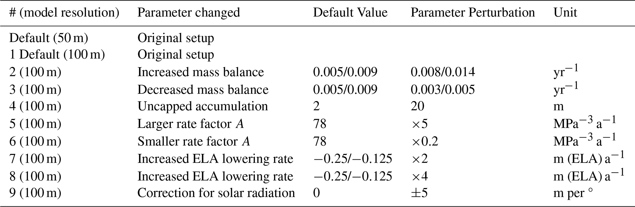
The choice of parameters is intended to give a broad picture of the uncertainties associated with our assumptions. These assumptions mainly concern the assumed linear SMB gradient, maximum accumulation, ice rigidity due to isothermal ice, and steady-state glacier geometry (simulations 2–9, Table 1). As the same mass-balance gradients are used over the whole Alps, variations of these gradients are applied to capture the full range of uncertainty they may introduce (simulations 2 and 3). Additionally, a scenario without the maximum accumulation at 2 m is included to test the effect of unrestricted ice accumulation in high elevations (simulation 4). Ice rheology and the basal boundary conditions were identified as additional uncertainties affecting ice volume estimates, especially given the assumption of isothermal ice rigidity. The analysis focuses on varying the rate factor A (simulations 5 and 6, Table 1), although various other parameters, such as for sliding conditions, could impact ice flow. The glaciers during the maximum extent of the LIA have probably not been in steady-state, so the effects of faster change in ELA are tested (simulations 7 and 8, Table 1). Finally, and in response to a modelled difference in the standard run between north and south exposed glaciers, we test a newly proposed correction for the exposure of the glacier surface to solar radiation, which includes aspect and slope in relation to latitude (also added as simulation 9 in Table 1).

Table 1 Parameter perturbations for the sensitivity analysis. Apart from the parameters listed, the simulation parameters do not differ between the simulations. The mass-balance gradients are specified with accumulation and ablation gradients. The simulation with uncapped accumulation is capped at 20 m, a value that is not reached in the Alps. The ice softness factor A is used as a rate factor in the Glen's flow law equations in Blatter (1995); Glen (1955). The ELA-lowering rates (for simulations 7 and 8) are given for intervals between 4000 and 3000 and 3000 to 1750 m a.s.l. The correction factor of the sun incidence angle (simulation 9) was only determined after evaluating the default simulations and corrects the ELA directly per grid cell relative to their surface angle deviation compared to a flat surface. The complete parameter settings can be found in the appendix (Table B1). Note that mass-balance gradients have the additional unit of m (ice accumulation/ablation) per m (elevation deviation from ELA) per year.

2.6 Climate data for further analysis

For evaluation purposes only, we use temperature and precipitation of the gridded pre-industrial climate snapshot simulation at 2 km resolution performed by Russo et al. (2024) using the Weather Research and Forecasting (WRF) regional climate model (Skamarock et al., 2008; Powers et al., 2017). The WRF pre-industrial climate snapshot is assumed to be suitable for comparison with the ELAs from the LIA, as this climate represents the mean climatic conditions.

The climate data is interpolated to the grid resolution of IGM (50 and 100 m resolution). The air temperature is adjusted to the actual surface using the elevation difference between the climate model surface and the glacier model surface, applying a lapse rate of 6 °C per kilometres (similar to Rabatel et al., 2013, and also supported by climate-model snapshot from Russo et al., 2024). No correction for precipitation with changing elevation is made. Using the empirical glacier outlines as a mask, we extract the annual precipitation by taking the median over all grid cells inside the glacier mask, or only the precipitation in the accumulation area when we mask for cells higher than the ELA. Additionally, the temperature at the ELA is obtained from the median of grid cells within the ±100 m elevation band bracketing the ELA. This ELA temperature is determined for annual and summer temperatures, with the latter using only June, July, and August data.

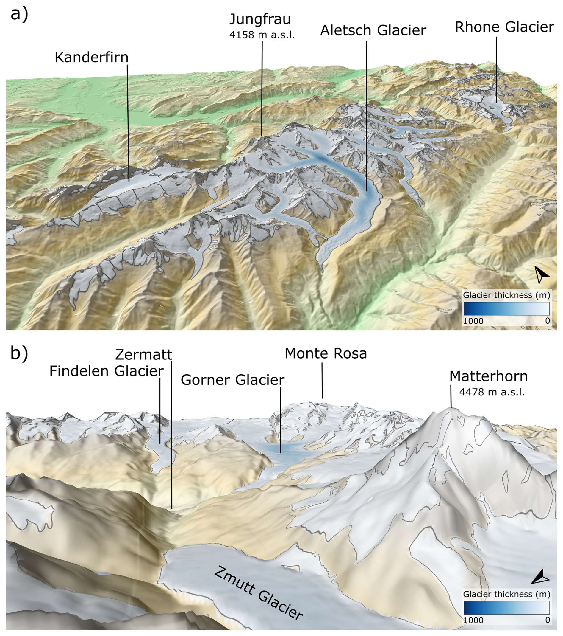
Figure 1 Two example 3D-scenes showing modelled glacier surfaces (white) and modelled thickness (blue shading), along with their empirical corresponding LIA-outlines (black lines, Reinthaler, 2024), which are used as target for the model output. The surface reconstruction is a mosaic of time-independent LIA maximum extent. (a) Central part of region 6 (Bernese Alps, Switzerland). (b) South-eastern part of region 5 (Pennine Alps, Switzerland/Italy). DEM modified after Japan Aerospace Exploration Agency (2021), Cook et al. (2023).

3 Results

3.1 Reconstructed glacier geometry

The main result of the study is a reconstruction of glacier surface geometries over the entire Alps that match the LIA terminus extents as given by the empirically mapped outlines (Reinthaler, 2024). An example of 3-dimensional views on such glacier surfaces are shown for the Aletsch region and the Matter valley in Fig. 1. The entire reconstruction represents a mosaic of 4094 individual glaciers (100 % of all mapped glaciers of the Alps) longer than 50 m during the LIA. Since the empirical outlines were used as model targets, the glacier areas between this study and that of Reinthaler and Paul (2025) are identical. In regard to volume, therefore, the critical variable is the ice thickness. Our physics-based model approach results in an Alps-wide glacier volume of 283±42 km³ during the LIA, while Reinthaler and Paul (2025) arrive at 280±43 km³. While overall volumes converge, regional variations persist, which are addressed in the Discussion.

The obtained volume for each glacier in the Alps shows a clear log-log relationship to both length and volume, respectively (Fig. 2). A total of 193 glaciers (<5 %) of all mapped glaciers could not be modelled as they were too small (not covering one complete grid cell of 50 m lateral length) and hence no volume or ELA estimate could be produced. The summed area of these not reconstructed glaciers is 1.2 km², corresponding to 0.03 % of the total glaciated area of 4203 km² estimated by Reinthaler and Paul (2025) for the LIA in the Alps. Among those successfully modelled, 854 glaciers (21 %) have areas larger than 1 km². 422 glaciers (10 %) have volumes greater than 0.1 km³. These 10 % of the largest glaciers make up 80 % of the total ice volume (283±42 km³) during the LIA.

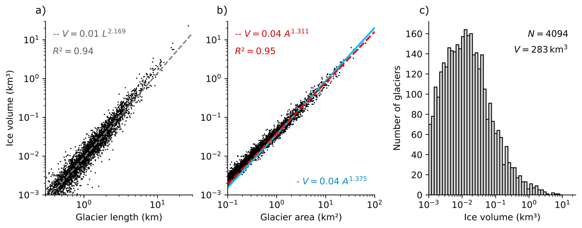
Figure 2 Power-law relationships between modelled ice volume V and (a) glacier flow line length L and (b) empirically mapped glacier area A (Reinthaler and Paul, 2025). Glaciers with areas smaller than 0.1 km² are excluded and not shown or used in the regression. The red dashed line represents a direct linear fit to the data, while the blue line represents a fit using a fixed exponent λ=1.375, following Bahr et al. (2015). (c) Histogram of the modelled LIA glacier volume distribution with total number of N=4094 glaciers and a total volume V=283 km³. Note that volumes below 0.01 km³ (generally corresponding to areas below 0.3 km²) are slightly overestimated due to the model's 50 m grid resolution. (A list with the ice volumes of the 60 largest glaciers is presented in Table , the full list is available with the data given in the data availability section.)

3.2 Alps-wide ELA per glacier

Our Alps-wide ELA reconstruction reveals both regional (between mountain ranges and valleys) and local patterns (between adjacent glaciers) (Fig. 3). As noted earlier, our modelling approach involved simulating each glacier's response to the ELA change until it matched its documented maximum length during the LIA. Regionally, ELA values are lower (average <2700 m a.s.l.) in the north-western Alps (northern part of region 3 and region 4), in the north (regions 6, 7) and north-eastern Alps (regions 12, 14, Fig. 3). On the other hand, ELA values are higher (average >2700 m a.s.l.) in the south-western Alps (regions 1, 2 and southern part of 3), the southern Alps (regions 5, 11) and in the inner-alpine valleys (regions 9, 10). Comparing regionally, median ELA values can differ up to 500 m (e.g. region 5 to region 4 or 14, Fig. 4). On a local scale, south- and north-facing glaciers have distinctly different ELA values (ca. 200–300 m difference, Fig. A1). In addition, we find individual glaciers that deviate from regional median ELA with more than 600 m difference to neighbouring glaciers which will be discussed later (e.g. very high or low ELA values, see inset region 5 Fig. 3, lower right corner).

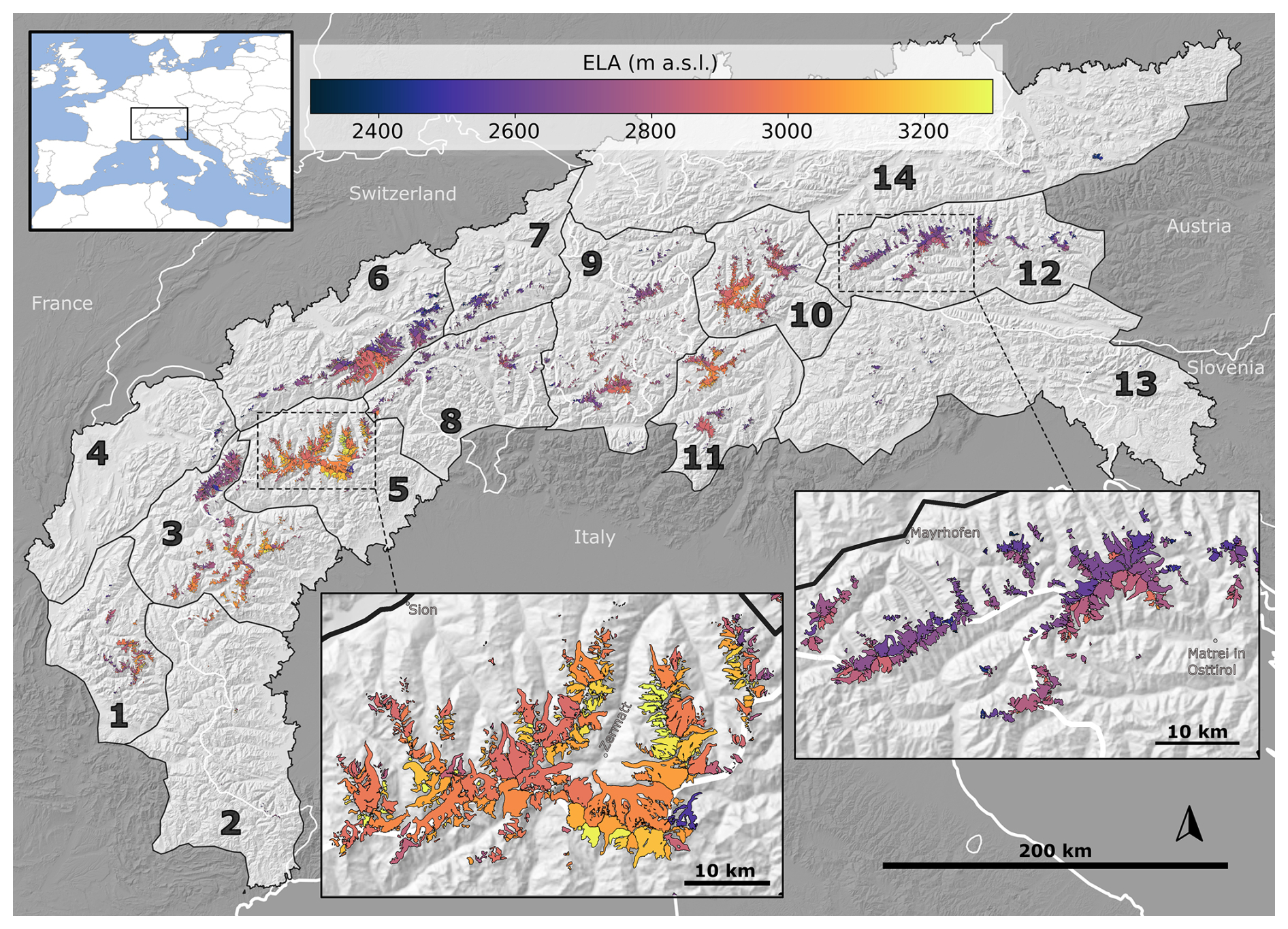
Figure 3 Map of the entire Alps with all model-derived ELAs using the outlines from the LIA (Reinthaler, 2024). The 14 regions are taken from the International Standardised Mountain Subdivision of the Alps (Marazzi, 2004), also used for comparisons by Sommer et al. (2020) and Reinthaler and Paul (2025); for region names see Table B2. The background map shows the shaded relief optained from the 30 m resolution AW3D30 DEM (Japan Aerospace Exploration Agency, 2021) with present-day glacier removed using the contemporary ice thickness reconstruction by Cook et al. (2023). (A list with the ELA values of the 60 largest glaciers is presented in Table , the full list is available with the data given in the data availability section and a version of the map in high resolution is available in the Supplement (see Fig. S1).)

3.3 Parameter sensitivity analysis

Additional simulations with variable ice-flow and climate parameters were performed to assess the sensitivity of the resulting glacier-specific volumes and ELAs. While the resulting volumes proved sensitive to these parameter changes, the glacier-wise ELAs remained largely stable across all sensitivity runs. The additional sensitivity simulations are illustrated using box plots showing the range of ELAs per region that can be compared with the default simulations (Fig. 4). The ELA differences between the regions are higher than the differences observed between the sensitivity simulations with almost identical medians and inter-quartile ranges (Fig. 4).

The sensitivity analysis indicates an uncertainty of up to 14 % of the total ice volume compared to the 283 km³ from the default run (Fig. 5). A volume change of +0.7 % is observed when reducing the model resolution to 100 m. Note that an additional run performed with even lower 200 m resolution gave a volume of 305 km³ which is about +8 % compared to 50 m resolution and could indicate a threshold of required minimum resolution to accurately resolve Alpine valley glaciers. Higher total ice volumes are associated with configurations featuring increased mass balance (+9 %), unrestricted maximum accumulation (+3 %), decreased rate factor (A×0.2, +12 %), and non-steady-state advance conditions where glaciers are in less equilibrated state in respect to the ELA change (Fig. 5). In contrast, lower volume estimates result from decreased mass balance (−11 %) and increased rate factor (−14 %).

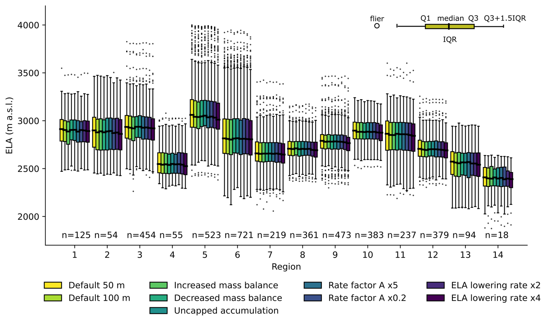
Figure 4 Box plots of the regional range of ELA values, showing also all distributions from the sensitivity analysis (simulations 1–9, see Table 1). The boxplot visually summarizes data distribution, with the box spanning the interquartile range (IQR) between the first (Q1) and third quartiles (Q3), the line inside the box marking the median, whiskers extending to 1.5 times the IQR to indicate variability, and individual points (fliers) representing possible outliers beyond the whiskers.

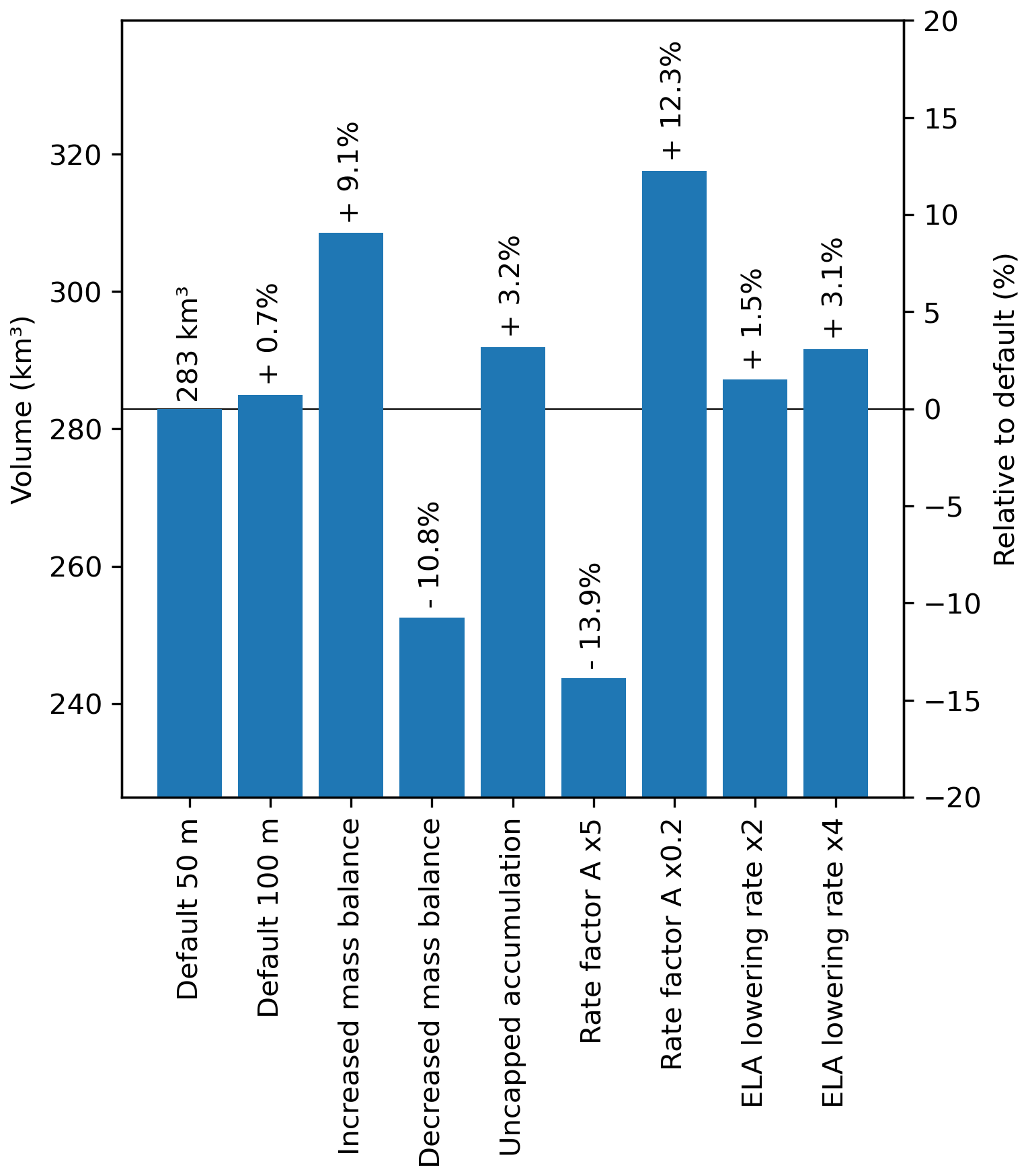
Figure 5 Total LIA glacier volumes and percentage deviation for the different sensitivity simulations relative to the default 50 m simulation (horizontal line). The volume difference to 100 m resolution is small (+0.7 %), volume differences for increased mass balance gradients and uncapped accumulation are positive and for decreased mass balance gradients are negative. Total volumes are negative for the increased rate factor A (increased ice softness) ×5 and positive for the decreased rate factor A×0.2, resembling stiffer ice rheology. Volume differences for the two faster ELA lowering rates are smaller than for other settings. Cf. Alps-wide glacier volume in 2015 and 2020 estimated at approximately 100 km³ (Cook et al., 2023; Reinthaler and Paul, 2025).

The ELAs computed with 50 m resolution do not significantly differ from the the same default model run at 100 m resolution (p value >0.05 for all regions). For the additional sensitivity runs, only the fastest tested ELA lowering rate (1 and 0.5 m a⁻¹) is significantly lower than the 100 m default simulation (p value <0.01). In the regional comparison, the significant difference of this fastest ELA lowering rate to the default 100 m simulation is given in regions 9 and 10 (p value <0.05).

4 Discussion

4.1 Reconstruction of 3D glacier geometry with a high-resolution ice-flow model

In our study, we simulate glacier flow in 3D using higher-order ice-flow physics at a resolution of 50 m. We perform in total ten simulations including two default simulations at 50 and 100 m resolution, seven sensitivity simulations for testing different parameters and one additional simulation with a newly proposed correction for aspect. For each simulation, we divide the European Alps in 14 subregions, to avoid exceeding the GPU memory limit (24 GB). Nevertheless, the regions still cover between 500 000 and 6.6 million grid cells. Comparable large-scale, 3D simulations and with such a fine resolution were previously considered unachievable (Zekollari et al., 2022).

Our estimate of modelled glacier volumes during the LIA across all regions of the Alps (283±42 km³) is similar to the GIS-based reconstruction of 280±43 km³ by Reinthaler and Paul (2025). There is a large interregional variability with respect to ice volume. Hence, average glacier thickness per region is used for comparison, which is the modelled ice volume divided by the empirically mapped glacier areas (Fig. 6). The regional average glacier thickness can be compared with results of Reinthaler and Paul (2025). In regions with glaciated area larger than 10 km², differences in mean average ice thickness are smaller than 6 m ($<\pm \mathrm{10}$ %). However, in regions with small glaciated area (<10 km²) differences in mean average ice thickness can be bigger (up to 14 m or +30 %) compared to Reinthaler and Paul (2025). Regions with small glaciated area have more smaller glaciers in which ice thickness is often exaggerated. The only few grid cells of a small glacier impedes realistic ice dynamics between adjacent cells, artificially inflating the simulated ice thickness in these areas. Taking all regions together, the IGM modelling approach allows an Alps-wide 3D glacier reconstruction at a resolution of 50 m, with results that are consistent with reconstructions not based on flow modelling (Reinthaler and Paul, 2025).

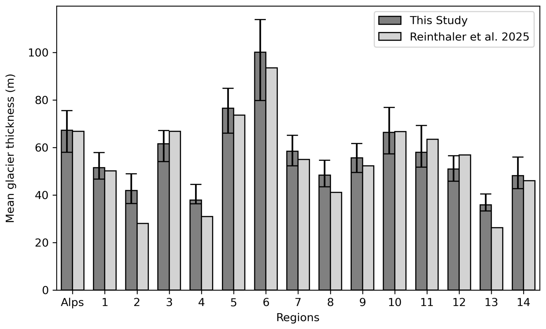
Figure 6 Modelled mean glacier thickness for the entire Alps and for each region at the LIA maximum glacier position, compared to the GIS-based reconstruction of Reinthaler and Paul (2025). Thickness is calculated as the model-obtained volume divided by the area for each region, as defined by the glacier outlines. The error bars show the maximum and minimum values of all the different sensitivity runs. Full details on volumes and thicknesses for each region are provided in Table B2.

4.2 Power-law relationship for glacier size

Volume-area scaling methods are used, mainly due to the better availability of area data compared to volume measurements. This approach, which is supported by the mathematical framework of Bahr et al. (1997, 2015), expects an exponent of 1.375 and corresponds to the linear slope in a log-log plot. Our modelling result and linear interpolation comes to a slightly lower value of 1.311. Our slope would be even lower if we were to consider glaciers below 0.1 km² surface area in the curve fitting. Ice volume of such small glaciers is mainly overestimated in modelling, as we have already seen in the regional thickness comparison (Fig. 6). The limited number of grid cells hinders adequate ice flow between the cells, leading to thicker ice coverage in these areas. This behaviour has also been observed at other spatial scales and with other glacier models (Seguinot et al., 2018; Jouvet et al., 2023; Leger et al., 2025).

In conclusion, area-volume scaling is in good agreement with our 3D ice-flow model and the fit with Bahr's exponent would give a total volume of 287 km³ (+1.3 %). However, just a volume reconstruction falls short of the detailed insights provided by this study. Here, each glacier is modelled individually in 3D at 50 m resolution, producing also surface geomteries and related mass balances that go beyond standard volume estimates (Fig. 1).

4.3 Climatic and topographic impacts on ELA pattern

In addition to LIA glacier surface reconstruction, our model enables the corresponding ELAs to be inferred for each glacier. These ELAs are compatible with the glacier geometry at the point at which the modelled glacier length matches the empirical LIA lengths. As no climate forcing dataset was used, our model-derived ELA values can be compared with independent snapshot model data, as presented in Russo et al. (2024). This provides valuable insights into spatial variability of glacier ELAs and its potential drivers (Fig. 7 and Table B4 for all regression parameters).

4.3.1 Air surface temperature at the ELA

The mean annual air temperature at the ELA serves as an indicator of the general climatic conditions at the glacier (Ahlmann, 1924; Ohmura and Boettcher, 2018). A wide range of summer temperatures from −1 to 4 °C and is observed at the ELA, obtained from the LIA climate snapshot (Russo et al., 2024) in combination with our glacier surface elevation and modelled-derived ELAs. There is a clear trend (p value ≪0.01) towards lower temperatures at higher ELA, suggesting a similar vertical temperature profile at equivalent altitudes in all regions (Fig. 7). Since temperatures at the ELA are still quite variable, there must be other important factors influencing the glacier-specific ELA.

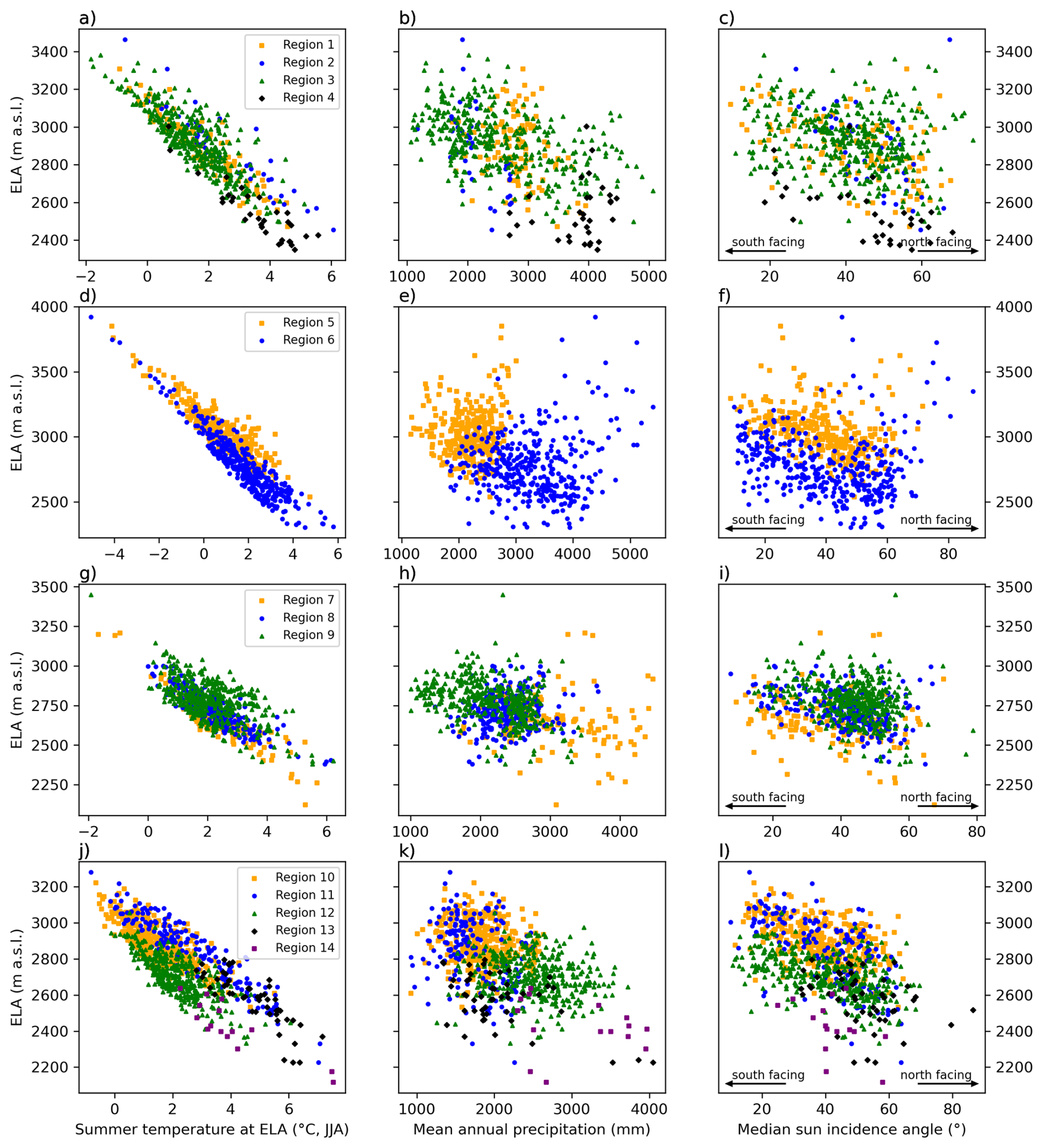
Figure 7 Climatic relationship with modelled ELA for the LIA in all regions for each glacier larger than 0.1 km². Climate data from pre-industrial climate snapshot (Russo et al., 2024). First column (a, d, g, j): ELA against mean summer temperature (June, July, August) at the level of the ELA. Second column (b, e, h, k): ELA against annual precipitation averaged over the whole glacier area and third column (c, f, i, l): ELA against glacier-averaged angle of solar incidence (median sun incidence angle). The median sun incidence angle serves as a proxy for incoming shortwave radiation, with the advantage of being straightforward and easy to calculate. With higher ELAs the mean annual temperature is lower (significant in all regions, p value <0.01). With higher precipitation, the ELA is lower (significant in all regions, p value <0.01, except regions 4, 7, and 14). ELAs are lower in more north facing glaciers (significant in all regions, except 13 and 14). We refer to Table B4 in the Appendix for linear regression parameters, p values and RMSEs for every region and all parameters shown here.

4.3.2 Precipitation and regional ELA patterns

Precipitation (data from Russo et al., 2024) over the glacier surface varies significantly, e.g. between the adjacent regions 5 and 6 (Pennine and Bernese Alps, p value ≪0.01) (Fig. 7e). Our reconstruction suggests that more precipitation allows for warmer ELA temperatures due to increased accumulation, a relationship recognised in previous studies (Ahlmann, 1922; Ohmura et al., 1992; Shi et al., 1992; Benn and Lehmkuhl, 2000). Thus, precipitation defines the temperature that can occur at the ELA. This is verifiable irrespective of considering annual or winter precipitation, or only precipitation in the accumulation area (Fig. A2). This consistency is likely due to the relatively uniform distribution of precipitation between seasons in the Alps that is measured in the 20th century (Isotta et al., 2014) and also modelled for the LIA by Russo et al. (2024). In conclusion, precipitation is a key factor in defining the broad regional ELA patterns observable in Fig. 3, but it alone cannot account for local variations between adjacent glaciers.

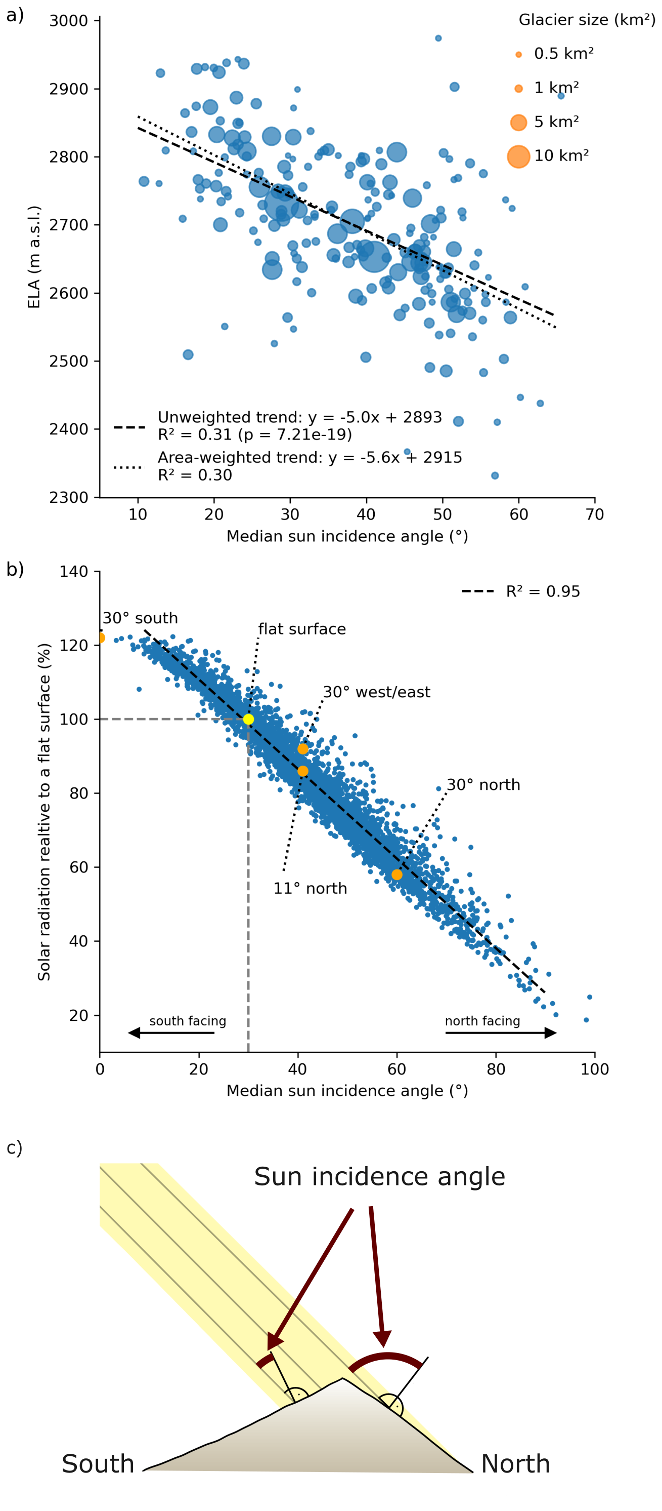
Figure 8 (a) Modelled ELAs against median sun incidence angle per glacier at midday in midsummer for region 12 (Tauern Alps West). The area of each glacier is indicated by the size of the marker. Trend lines are calculated using unweighted and area-weighted linear fits. (b) Median sun incidence angle against the total shortwave radiation, in relation to a horizontal surface for each glacier in the Alps (R²=0.95). The horizontal surface should by definition have an angle of 30° (grey vertical and horizontal lines, see Appendix C for explanation). Some distinct combinations of slope and aspect are shown as orange dots. (c) Sketch illustrating how the sun's incidence angle is defined. The actual calculation of the angle is performed in three dimensions. The median sun incidence angle is taken from the median of all grid cells of a glacier. An incidence angle of more than 90° means that this surface is in the shadow of its own surface during the highest position of the midsummer sun. Nevertheless, it is valuable to derive a value for steeply north-facing areas that receive only indirect solar radiation, as the insolation never reaches zero. Note that total solar radiation integrates every half an hour of sun radiation over a full year, which explains why east/west exposed surfaces have a higher total solar radiation than a surface with north aspect even with the same median sun incidence angle in (b).

4.3.3 Solar radiation and local ELA differences

On a local level, a pattern of ELAs becomes apparent, when comparing directly adjacent glaciers (Insets in Fig. 3). South-facing glaciers have significantly higher ELAs than north-facing glaciers (Regionally all p values <0.01 besides regions 13 and 14 with small sample sizes). This pattern can also be seen across the entire Alps (p≪0.01), although the influence of precipitation, temperature, and likely other factors, may account for the increased scatter of data points around the regression line (Figs. 8 and A1).

The effect of mean annual solar radiation is here approximated by calculating the angle of incidence of the sun ray at midsummer and midday averaged over the whole glacier surface (called the median sun incidence angle). This is a new proposed approach in this study, which yields an R² value of 0.95 and an RMSE of 4 % in a linear regression comparing to a full shortwave radiation calculation (Fig. 8b). Smaller solar incidence angles (more vertical sun rays towards the average glacier surface) generally lead to higher ELAs, a trend that, although not perfectly correlated, intuitively aligns with expectations from previous studies (Ahlmann, 1922; Ohmura and Boettcher, 2018). Thus, the median sun incidence angle per glacier can be seen as an approximation of the incoming shortwave radiation.

Our measure of the median sun incidence is more advanced than just using the aspect of the surface and is also better suited for almost flat surfaces. For two nearly flat surfaces tilted slightly to the south or north, the difference in the angle of incidence is small but the difference in aspect is large and therefore misleading. However, calculating the median sun incidence angle just requires simple trigonometric functions and the applied corrections is therefore as efficient as calculating aspect (see Appendix C for more details). This is in contrast to the more complex and computationally expensive determination of the total incoming shortwave radiation integrated over a full year.

The observed trend in ELA with the median sun incidence angle provides an opportunity for correcting the effect solar radiation in a mass balance model. For the example of the Tauern Alps West (Region 12) shown in Fig. 8 a we obtain 5 m ELA change per degree of sun angle. We apply such a correction in our surface mass balance parametrisation and re-run the entire modelling reconstruction (simulation 9 in the sensitivity analysis). We then find that the aspect related local variations in particular within a single mountain massif are reduced to have no statistical significance (Fig. A3). However, while the general trend from the incident angle is removed with this ELA correction, substantial glacier to glacier variations up to several hundred metres elevation remain due to other local factors such as avalanching, relief shading, calving or wind erosion and deposition of snow.

4.4 Model sensitivity is dominated by ice thickness

The sensitivity analysis in this study reveals no significant sensitivity for the ELA reconstruction and an uncertainty of up to 14 % for the ice volume estimate. We tested for a wide range of plausible perturbation values like ice softness (rate factors), different mass balance gradients, and faster non-steady state glacier advances.

Since the glaciers are modelled to have a length corresponding to the empirical outlines by Reinthaler and Paul (2025), the different volume estimates arise from different mean ice thicknesses. Therefore, a larger volume in the sensitivity analysis is observed where the glaciers are thicker which explains why volume estimates are higher for more rigid ice (small rate factor A×0.2 or increased accumulation). Here we chose a rate factor for ice that is five times more rigid (A×0.2) likely representing the upper bound of this range (corresponding to an ice temperature of approximately −10 °C; Cuffey and Paterson, 2010). Increased accumulation (due to increased mass balance or uncapped accumulation) has the effect that more mass turn over occurs, which in itself can only be done by increasing the glacier thickness, i.e. the ice discharge, under otherwise identical conditions. Conversely, there are various factors that result in thinner ice. This can be on one hand a more deformable ice (5×A). On the other hand, less accumulation and ablation also means that less mass has to be transferred over the whole glacier, which is associated with thinner ice. Various factors lead to thicker or thinner glaciers, which determines the volume estimation. Thus, experiments that change ice rheology or basal sliding would have similar effects on the modelled ice volume. With this reasoning, the number of sensitivity simulations for ice volume could be reduced, as less basal sliding or more rigid ice would lead to the similar results, namely more volume and vice versa for more sliding and softer ice.

The non-steady-state sensitivity simulations (ELA lowering rate ×2 and ×4) provide additional insights into glacier behaviour under transient conditions (+1.4 % and +3.1 % ice volume). Specifically, these simulations model less equilibrated glacier geometries, reflecting a delayed response of glacier tongues to increased mass (thickness) in the upper regions driven by the ELA lowering (Fig. 5). In these non-steady-state simulations, the higher mass in the glacier's upper part has not yet propagated to the glacier tongue. Since the target in the modelling approach is to match glacier length, this results in slightly higher modelled ice volumes and slightly lower ELA values (Figs. 5 and 9). The ELA values remain insignificantly lowered across all regions in the sensitivity run with two times faster ELA lowering (p>0.05, Fig. 9) and appear significantly lower for ELA lowering rate ×4. In conclusion, transient non-steady-state simulations may affect the reconstructed glacier geometry, as advancing glaciers tend to have a greater volume than stable or retreating glaciers of the same length. This effect is probably more pronounced for larger glaciers, which have longer response times. Moreover, our steady-state ELAs for the LIA are most likely higher in elevation than a specific short-term excursion during the LIA maximum could have been. However, it is worth noting that in reality the LIA spanned over 500 years, and not all glaciers reached their maximum extent simultaneously, nor did they all do so at the end of the LIA. The reconstructed geometries shown here depict an approximate maximum configuration around 1850, but this may not apply to all glaciers (Holzhauser et al., 2005; Nicolussi et al., 2022).

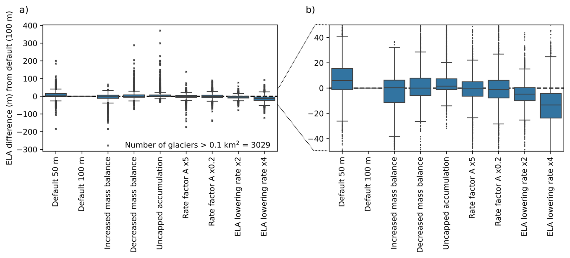
Figure 9 Deviation of ELA values from the standard 100 m resolution run for the different sensitivity experiments for all glaciers larger than 0.1 km². The first box plot reveals insignificant higher ELAs with higher 50 m model resolution and differences on average of less than 30 m in ELA (p value >0.05). Between all model runs with 100 m resolution, only ELAs with ELA lowering rate ×4 shows a significant deviation from Alps-wide ELA values (p value <0.01). (a) The full range box plots showing all outliers. (b) Zoomed version. Each boxplot visually summarizes data distribution, with the box spanning the interquartile range (IQR) between the first (Q1) and third quartiles (Q3), the line inside the box marking the median, whiskers extending to 1.5 times the IQR to indicate variability, and individual points (fliers) representing possible outliers beyond the whiskers.

4.5 Outliers in the ELA reconstruction: avalanche-fed glaciers and high-altitude ice patches

Outliers in this context are defined as glaciers with ELAs that deviate substantially (>200–600 m) from their adjacent glaciers or exhibit unusually high ELAs (above 3500 m a.s.l.). These outliers are notable on the ELA map, such as very high ELA points next to larger glaciers with lower ELAs (Fig. 3). Factors contributing to these outliers include physical model limitations, particularly in areas with debris cover, steep rock walls, or high-altitude glacier fields like hanging glaciers, where accumulation and ablation mechanisms differ from typical melt-driven processes. Therefore, the outliers represent physically atypical glacier configurations rather than genuine model errors.

Debris cover is a key factor that significantly alters ablation patterns, but was neglected in this study. In future work, debris cover could be integrated by modifying surface melt parameters according to assumed debris abundance and thickness – an aspect currently under development for IGM (Hardmeier et al., 2025). We assume that debris cover is of minor importance for the Alps-wide results presented in this study because not many glaciers in the Alps are covered by debris today and even less so during the LIA (D'Agata and Zanutta, 2007; Kirkbride and Deline, 2013; Mölg et al., 2019; Kropáček et al., 2024). However, we observe some prominent unexpected low ELAs of present-day debris-covered glaciers. A notable example is Ghiacciaio del Belvedere (Belvedere Glacier), which has a modelled ELA of 2540 m a.s.l. during the LIA and therefore a much lower ELA than all nearby glaciers (LIA ELA >3000 m a.s.l. Fig. 3 inset region 5, lower right corner). Ghiacciaio del Belvedere is known to have been less debris-covered during the LIA than it is today (Kropáček et al., 2024), an observation that argues against lack of debris cover parameterisation as a reason for the exceptionally low ELA. Yet, Ghiacciaio del Belvedere has head walls with more than 30° slopes (for more than 1000 m elevation difference) with possible strong avalanche influence, which could lead to an underestimation of accumulation in the lower regions of the glacier (Kropáček et al., 2024). It is rather complicated to disentangle the dominant influence of high relief, which causes potential debris cover (through increased rockfall) and avalanche-fed additional snow accumulation, the two of which potentially go hand in hand anyway. In addition, Ghiacciaio del Belvedere shows surge-like behaviour (Haeberli et al., 2002; Brodský et al., 2024), a process not accounted for in our modelling.

In addition to neglected accumulation processes, our model also likely misses some ablation processes, particularly for small glacier patches and firn fields near mountain peaks with very high modelled ELAs (>3500 m a.s.l.). These patches experience additional ice loss mechanisms in nature, such as ice break-off (dry calving) or wind erosion. Ice break-off and wind erosion reduce accumulation or exhibit additional ablation that is not accounted for in our surface mass balance parametrisation. Other outliers in the ELA reconstruction come from the automatically generated flow line that does not extend to the glacier's lowest elevation. This is partly because some glacier outlines are delineated as separate units, despite the ice merging with neighbouring or downstream glaciers.

In summary, our modelling experiment is likely to underestimate ELAs for debris-covered and avalanche-fed glaciers during the LIA and overestimate them for small ice and firn patches in high-altitude regions or some glaciers with confluences. More generally, such local deviations in modelled ELAs from the regional signal could potentially be further explored to provide information about processes that are neglected in our simple elevation dependent surface mass balance parametrisation. However, the surface reconstruction and resulting volumes are not much affected by this, as these glaciers are rare or very small and, therefore, contribute little to the overall volume.

4.6 Comparison to palaeo-glacier ELAs

We compare our approach of optained ELA values, that are 3D-modelled and ice-physics consistent matching empirical glacier outlines, with the well-established palaeo-ELA reconstruction methods that only require minimal data or GIS based approaches (Fig. 10). These methods can be broadly categorised into three groups with different data input requirements.

Firstly, models that do not require knowledge of the detailed former shape of the glacier include THAR (toe-to-headwall ratio, e.g. in Meierding, 1982; Benn et al., 2005; Rea, 2009). Based on the literature we use here a THAR of 0.5 (mid-elevation). The THAR ELA calculation generally has a good fit (linear regression R²=0.89) to our glacier model ELA, but some larger glaciers result in up to 500 m different ELA values (positive and negative) than the model derived ELAs (Fig. 10a). This discrepancy is probably due to the hypsometry and definition of mass balance gradients for our ELA model, where the accumulation area is usually larger than the ablation area (Benn and Lehmkuhl, 2000). Notable examples include the relatively large glaciers with high relief in the Mont Blanc region (Glacier de la Brenva, Glacier du Miage) and Monte-Rosa region (Ghiacciaio del Belvedere). These glaciers often extend to very high elevations and have glaciated head walls, leading to higher THAR ELAs when the elevations are derived from the empirical outlines used in this study (Reinthaler and Paul, 2025). A ratio lower than 0.5 is also suggested by Meierding (1982), which could lower the THAR ELAs. In summary our analysis shows that the THAR ELA is highly dependent on the shape of the glacier, and is less appropriate for high reliefs (similar to Porter, 1977; Benn et al., 2005).

Secondly, models that require some knowledge of glacier geometry (at least outlines) include the AAR (accumulation-area ratio). The AAR value chosen here is 0.67. Comparison of AAR ELAs and modelled ELAs shows some differences, but similar fit is obtained (linear regression R²=0.91) than for the THAR. Nevertheless, glaciers originating from high elevations in the Mont Blanc region (e.g. Glacier des Bossons) are deviating from model-derived ELAs by more than 300 m (Fig. 10b). Similar to THAR ELAs, high relief can be problematic for calculating AAR ELAs. Some processes are not taken into account when using these ratios, such as reduced accumulation on high mountain peaks due to wind and high melt due to very low lying steep tongues.

Lastly, methods like AABR (area-altitude balance ratio) need full knowledge of the glacier hypsometry and hence surface geometry. The here chosen AABR for the Alps is 1.29 (Oien et al., 2022). The AABR, which estimates ELAs iteratively based on elevation bands of the glacier surface, does not reduce the scatter to our modelled ELAs more than the less elaborate methods above (Fig. 10c, R²=0.90). The general slight positive offset (above the 1:1 line, Fig. 10) is probably due to the capped 2 m accumulation in our modelling approach resulting in lower ELA values. AABR does not rely on this assumption of maximum accumulation.

In summary, results from simple ELA reconstruction methods for glaciers generally agree well with those from our physically based approach. For some larger glaciers with high relief, THAR, AAR, and AABR can lead to unrealistically high ELA values. However, smaller glaciers also show deviations if the hypsometry is complicated, meaning no clear size threshold can be seen, at which point a certain method works better. For small, mostly regenerated disconnected glacier patches, the ratio-based ELA naturally falls between the highest and lowest elevation of the outline in all ELA calculation methods. This is not the case in the ice-flow model, where small glacier patches at low elevations are fed by ice from higher elevations (small glaciers below the 1:1 line, Fig. 10). In conclusion, these primary elevation or area-based relationships are less applicable to complex hypsometry, with e.g. ice-covered head walls and high relief. On the other hand, estimated ELAs from these methods also depend on the chosen ratio numbers.

The resulting Alps-wide ELA dataset for the LIA can prove useful for the larger palaeo-glaciolocial community by providing consistent physical ELA values for over 4000 (100 % of all mapped >50 m long) glaciers of the Alps for the pre-industrial LIA. Our physics-based results largely agree with simple, elevation-dependent ELA estimations but our model also shows robust estimates for complex, high-relief glaciers. The correlation between ELA and mean temperature or precipitation, which is both regional and Alps-wide (see Fig. 7), allows useful calculations to be made in the context of (palaeo)climate change (numbers for regression given in Table B4). The ELAs of larger glaciers are provided in Table  and data of all glaciers are provided as an attribute table in the shapefiles in the data availability section.

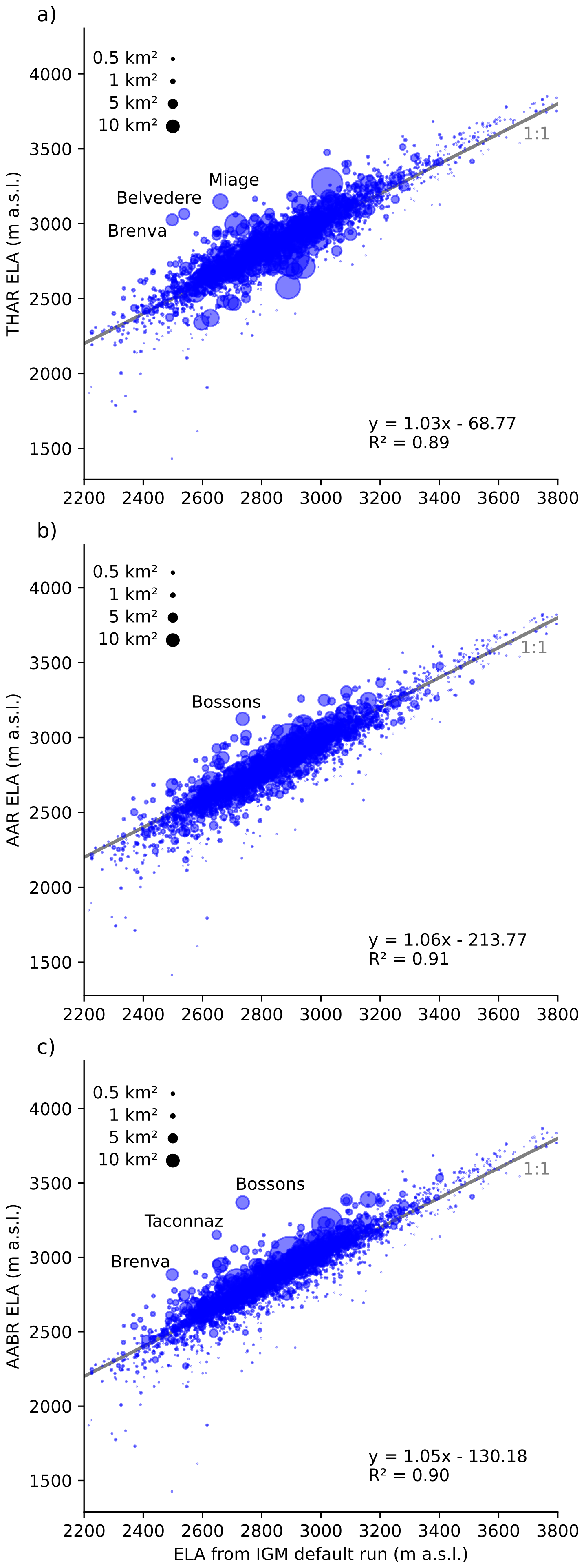
Figure 10 Comparison of modelled ELA using IGM to different palaeo-ELA reconstruction methods for the LIA glacier extent. Different methods for palaeo-glacier ELA reconstructions are tested here which are: THAR (toe-to-headwall altitude ratio, here THAR = 0.5), AAR (accumulation altitude ratio, here AAR = 0.67), and AABR (area-altitude balance ratio, here AABR = 1.29 (Oien et al., 2022)). Some glaciers mentioned in the text are labeled such as the glaciers in the high Western Alps (Region 3): Glacier de la Brenva, Glacier du Miage, Glacier des Bossons, Glacier de Taconnaz; and the glaciers in the high Pennine Alps (Region 6): Ghiacciaio del Belvedere. The gray line is the 1:1 line for orientation.

5 Conclusions

In this study, we employ the Instructed Glacier Model (IGM) to derive a new high-resolution (50 m) 3D representation of the geometry of Alpine glaciers at their maximum extent during the Little Ice Age (LIA). Our glacier surface and equilibrium line altitude (ELA) reconstruction is consistent with the physics of ice flow and with the principles of mass conservation and mass balance. ELAs are determined for each single glacier over the entire Alps (N=4094 glaciers). Thanks to the high spatial resolution, even small glaciers with an area of less than 1 km² (N=3218) are resolved. The total volume for all glaciers associated with our new glacier surface reconstruction amounts to 283±43 km³.

Results were achieved with an elevation-dependent mass balance model with separate linear mass-balance gradients for the accumulation and ablation areas, respectively. The ELAs obtained reveal regional and local spatial patterns that show clear correlations with climatic and topographic parameters. Regions with simulated depressed ELAs clearly match regions with increased precipitation. For north-facing glaciers, we obtain ELA values that are up to 500 m lower than for their south-facing neighbours. For correcting this effect of solar radiation, we propose a new approach by directly correcting the ELA by a factor based on the sun ray incidence angle at midsummer and midday. Nevertheless, the complex interplay between regional climate variables and local topographic factors warrants further investigation and highlights the challenge of modelling glaciers over entire mountain regions with a single-parameter configuration. Our new LIA ELA data provide valuable insights for future palaeo-glaciological studies. Furthermore, the modelling of glaciers constrained by geologically reconstructed palaeo-glacier lengths, as applied in this study, represents an improved and efficient method for reconstructing glacier surfaces of entire mountain regions that is fully consistent with the principles of glacier physics.

While we apply a strong reasoning for including climatic as well as topographic variables in surface mass-balance modelling, the applied model set-up has revealed challenges in explaining all observed spatial patterns in the ELA reconstruction results. Uncertainties exist due to poorly resolved climate parameters as well as general constraints of our approach, such as spatially non-variant model parameters. Simultaneous 3D modelling of all Alpine glaciers to their empirically reconstructed LIA maximum extent, driven by the same transient climate forcing, remains a goal for future studies. To achieve this, a dynamic, transient modelling approach would be required. This approach would involve a glacier-specific and highly detailed transient mass balance forcing including a spin-up, beginning several hundred years before the LIA. In this context, it is important to note that the outlines themselves do not represent a single, simultaneous maximum position for all glaciers (Reinthaler and Paul, 2025). Glaciers in different regions did not always reach their most advanced positions at the same time, and they re-advanced at different periods during the LIA (Holzhauser et al., 2005; Nicolussi et al., 2022).

A future approach to improve our modelling reconstruction framework could employ a more sophisticated surface mass balance implementation that directly incorporates precipitation and temperature inputs and more factors such as wind, avalanching, shortwave radiation or relief shading and debris cover. Although more complex mass balance scheme is already available in IGM, in the context of palaeoglaciology prior to the LIA, uncertainties in simple climate inputs such as precipitation and temperature may introduce more uncertainty.

Appendix A: Appendix figures

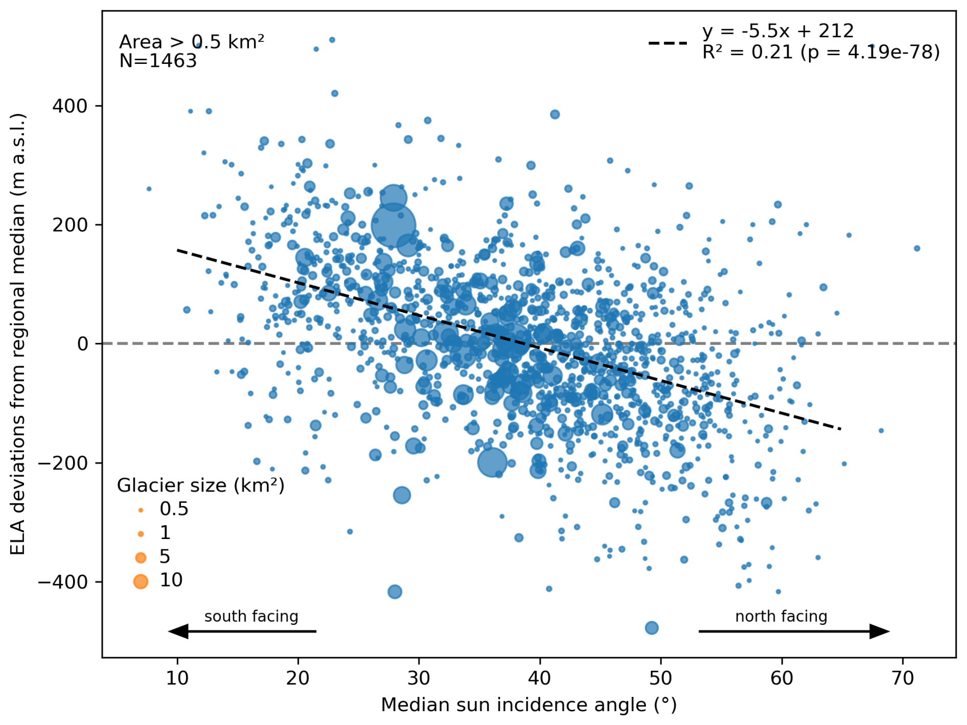
Figure A1 Modelled Alps-wide ELAs (difference to regional median) versus median solar angle per glacier at midday in midsummer (“median sun incidence angle”). The area of each glacier is indicated by the size of the marker. Although the linear regression trend is significant (p value ≪0.01), there is a rather large scatter. This is due to other factors such as precipitation, temperature, shading, avalanching etc. that affect the ELAs for each glacier differently. For better readability, only glaciers with areas larger than 0.5 km² are shown (N=1463). The trend with all glacier larger than 0.1 km² would result in a less steep slope (−4.63) but still significant trend (p value ≪0.01).

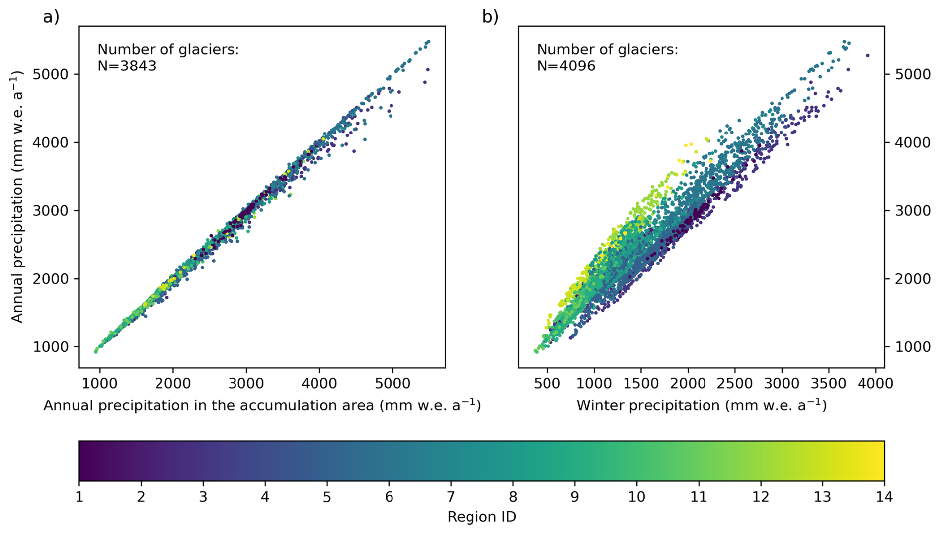
Figure A2 Comparison of mean annual precipitation versus (a) precipitation only in the accumulation area and (b) precipitation during the winter half-year from November to April. Each dot represents a glacier, coloured by region. All data are derived from climate simulations by Russo et al. (2024) and are given in mm water equivalent (w.e.) per year. (a) The resolution of the climate model is 2 km, which likely explains the minimal difference between the precipitation in the specific areas. More precipitation in the upper glacier area would have been expected. (b) Slightly less winter precipitation is observed in the north-eastern regions (12–14) compared to the south-western regions (1–3). However, the differences are not substantial, indicating that precipitation is relatively well-distributed seasonally across the Alps. The lower number of glaciers in (a) can be explained that not all glaciers have a dedicated accumulation area inside their empirically mapped outline. This is the case when the outlines have no elevation up to the ELA, as e.g. low regenerated glaciers were separately mapped but gain ice from higher elevations. Note that the modelled precipitation in this LIA snapshot simulation is likely to be higher than expected for areas at a higher elevation when the dataset is compared to today's expected annual precipitation.

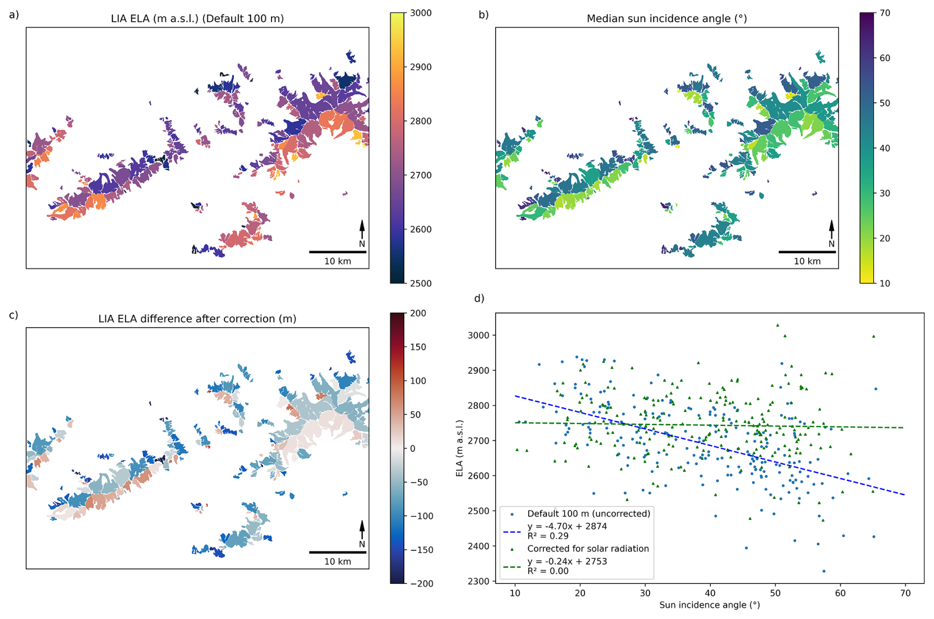
Figure A3 The test case of LIA ELA correction in region 12 (Tauern Alps West). (a) Uncorrected ELA map (default simulation at 100 m resolution) and mean sun angle (b) as initial data. Correction with 5 m ELA decrease per degree of sun angle increase, leaving flat surfaces at zero ELA correction. (c) Resulting ELA map differences between radiation-corrected forcing ELA and forcing ELA of default simulation and (d) ELA vs. sun incidence angle. The trend of higher ELA at lower sun angles has been corrected. Note that the forcing ELA is not the same as the effective ELA of the glacier once the ELA is corrected for the different incidence angles per grid cell.

Appendix B: Appendix tables

Table B1 Example parameter file for region 1 in the default 50 m simulation. Names for the input files and parameters to coarsen the input topography change when using other regions or resolutions. We reduced the learning rate of retraining and the frequency of retraining for the 50 and 100 m resolution by half (retraining the emulator slower and more often), which in our case means about 25 % more computation time compared to default values in IGM v 2.2.2. Full details about the model can be seen in the code-supplement and Jouvet and Cordonnier (2023), Jouvet et al. (2024).

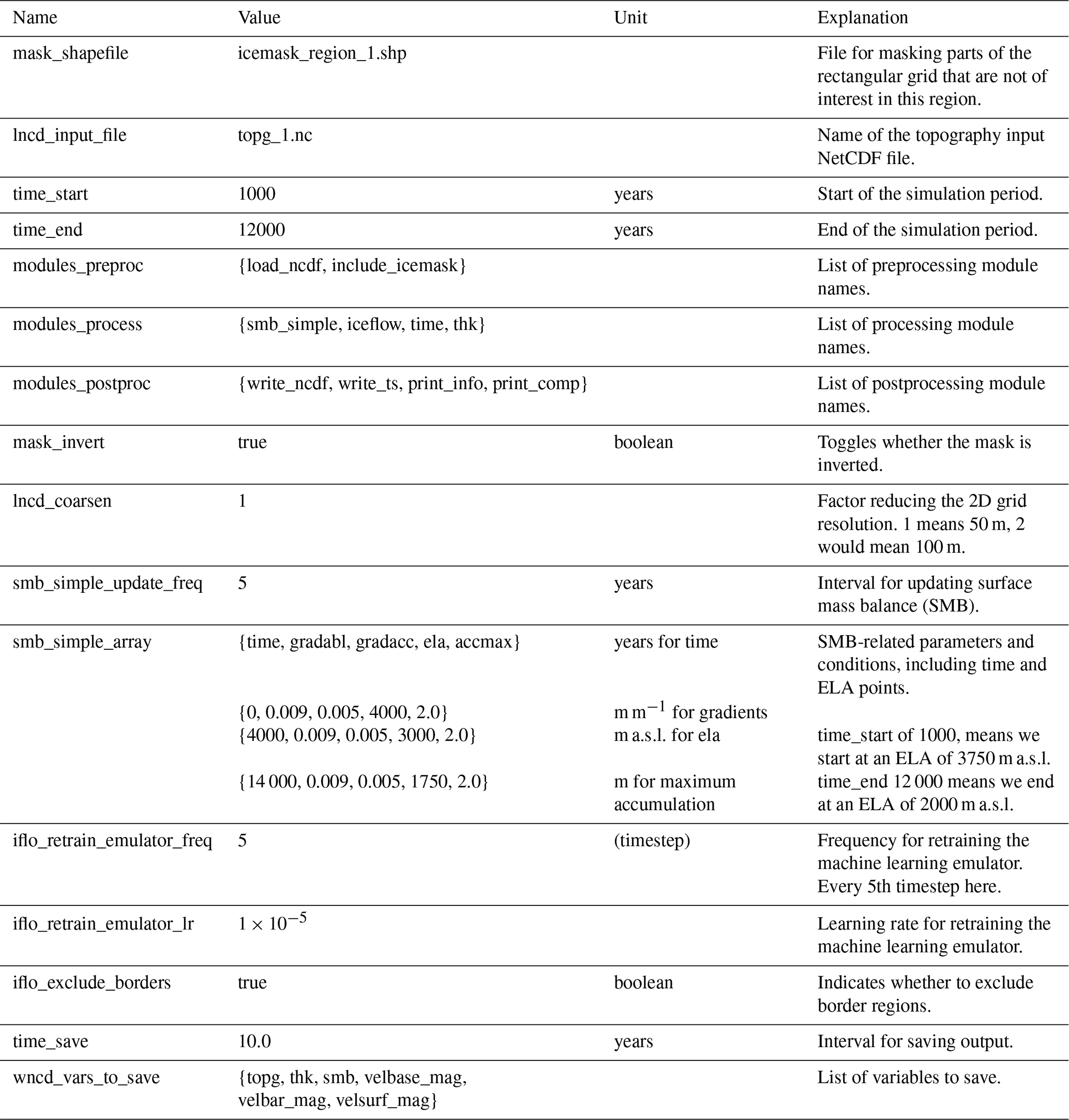
Table B2 Glacier volume and mean ice thickness (in brackets) for each region and Alps-wide, obtained from the modelled results of this study. First three columns are given by the dataset by Reinthaler (2024) and therefore the same for all simulations. The table presents the modelled LIA ice volume in cubic kilometers (km³) and the mean ice thickness in metres (m) for all sensitivity simulations, including default settings at 50 m and 100 m resolutions. All sensitivity simulations are done with 100 m model resolution (see Table 1).

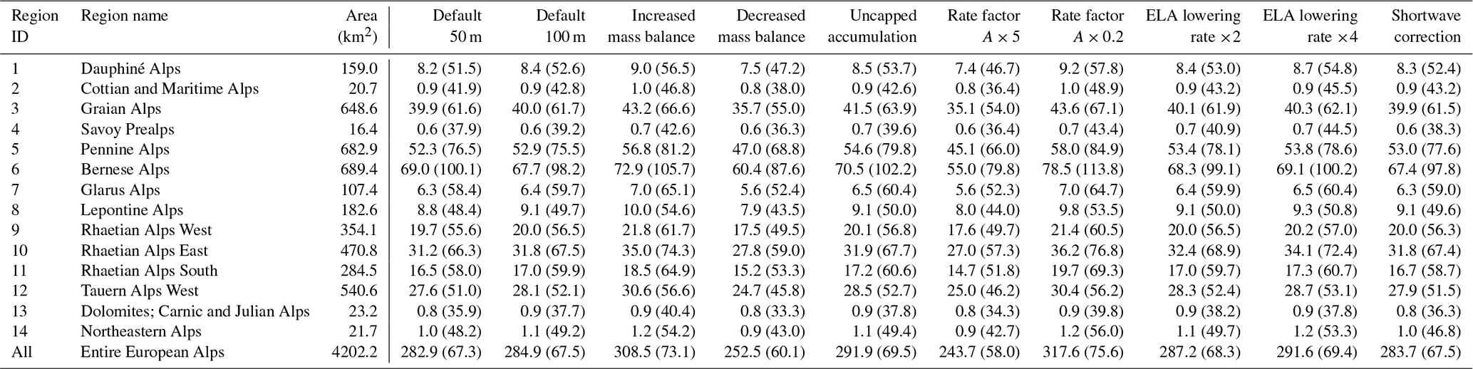
Table B3 Table of the 60 biggest LIA glaciers of the Alps by area (Area >10 km²). Note that, due to ongoing ice melt and glacier tongue disintegration, deviations between names of LIA glaciers and present day glaciers exist. Where applicable, we list present-day and former LIA main tributary glaciers. IDs, citation, LIA lengths and LIA areas are taken from Reinthaler (2024), LIA ice volume and LIA ELA added from this study.

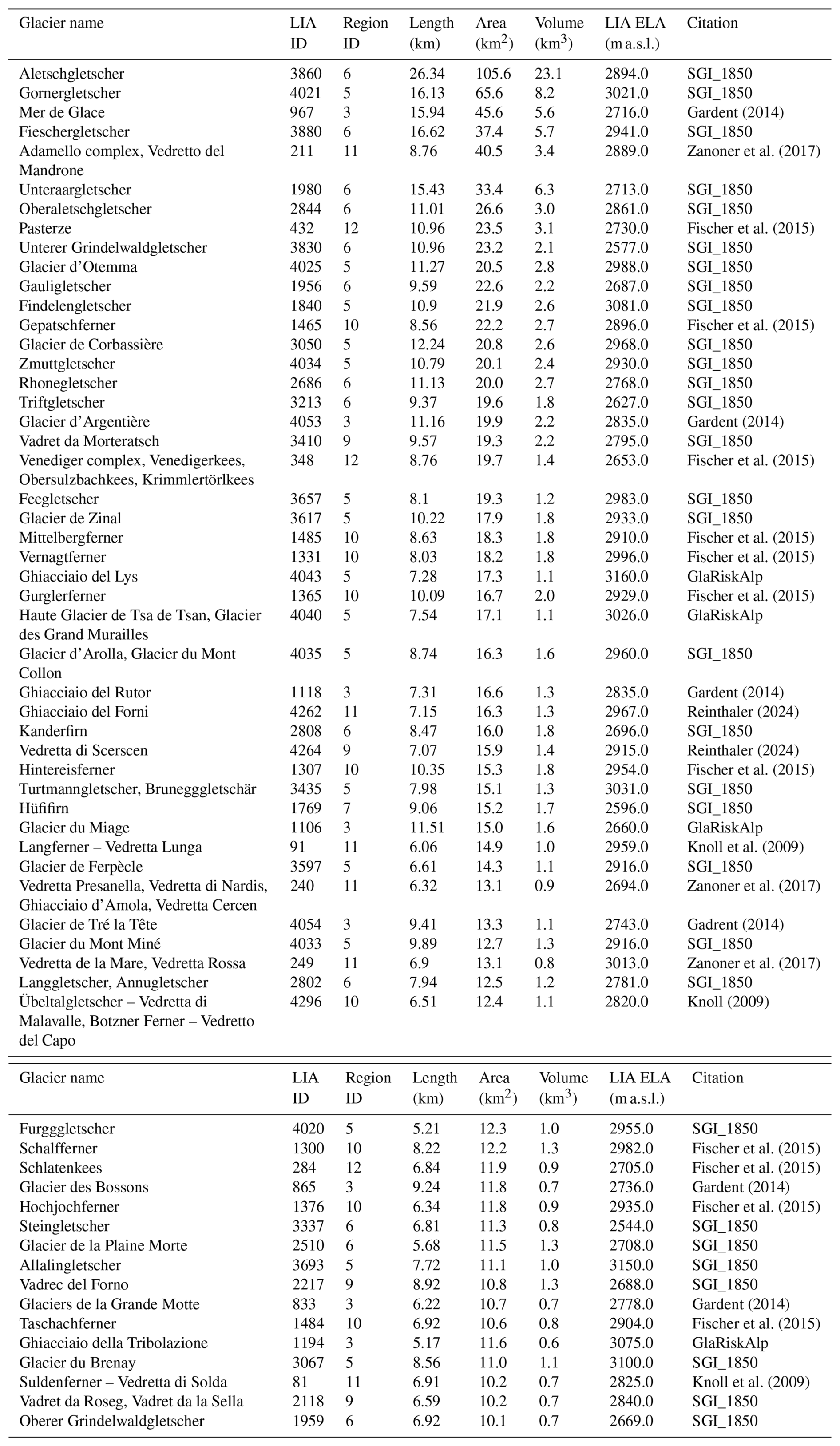
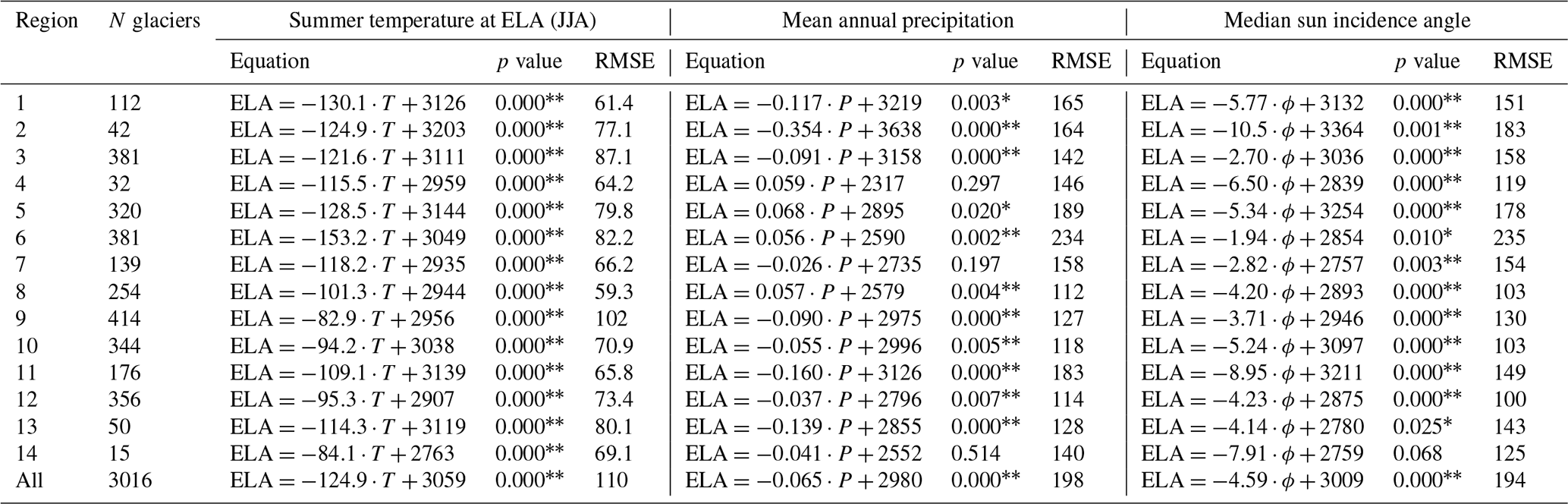
Table B4 Regression results for the climatic ELA relationship, by region and overall. The analysis only includes glaciers with an area larger than 0.1 km², corresponding to the data shown in the scatter plots of Fig. 7. The temperature data (refering to summer temperatures of June, July, August) and precipitation data are sourced from Russo et al. (2024). The median sun incidence angle is derived from the calculations in this study. The Alps-wide regression y intercept may be misleading due to significant regional variability. Where possible, preference should be given to regional regression y intercepts for more reliable insights. Note that the precipitation data from the climate model runs by Russo et al. (2024) are likely to be overestimated for most higher-elevation grid cells. * represents the significance level p<0.05; ** represents the significance level p<0.01.

Appendix C: Correction for solar irradiance

Cumulative shortwave radiation (clear sky radiation) integrated over a year shows good correlation (R²=0.95) to the sun incidence angle of midsummer sun (Fig. 8b). However, incoming shortwave radiation of all possible sun positions over a year is computationally intense. This is true particularly where the glacier surface may change and the incoming radiation needs to be recalculated after a period (updating frequency of the surface mass balance). On the other hand, sun incidence angle of midsummer sun is quick to compute using a few trigonometric functions which are given below. Thus, we replace the computationally intensive correction of the cumulative shortwave radiation by a simpler approach that relies on surface slope and aspect (angle of sun incidence) and assumes one single sun position: at mid June (midsummer) at midday. Midsummer and midday in the European Alps corresponds to a sun position in the south and 60° above the horizon. Angles of incidence are defined to the surface normal, which gives 90° − 60° = 30° sun incidence angle for a flat surface by definition (see also sketch in Fig. 8c). In the following we calculate the glacier-wide median of this incidence angle using every grid cell inside the glacier outline and refer to it as “median sun incidence angle”.

Our surface mass balance model is adapted in simulation 9 by this ELA correction based on this sun incidence angle (Table 1). When forcing the single global ELA, a hypothetical ELA is calculated from this radiation correction for every grid cell which is then (as usual) taken into the mass balance model that calculates the mass balance depending on the elevation difference of the surface to the ELA (using the mass balance gradients). To not change any ELA value for flat (horizontal) surfaces, we account for the deviation angle of the incoming sun ray vector.

The angle deviation dϕ is calculated as the difference in the sun incidence angle ϕ compared to a flat surface

$$\begin{array}{}\text{(C1)}& \mathrm{d}\mathit{\varphi }={\mathit{\varphi }}_{\text{flat\_surface}}-\mathit{\varphi }.\end{array}$$

This deviation is used to calculate the ELA correction, accounting for variations in solar radiation due to topography. The ELA correction (x, y) is then calculated as

$$\begin{array}{}\text{(C2)}& \begin{array}{rl}& \text{ela\_correction}=\mathrm{d}\mathit{\varphi }\\ & \times \text{ela\_correction\_per\_degree\_sun\_incidence}\end{array}\end{array}$$

The sun incidence angle ϕ is the angle between the normal vector of the surface n and the incoming sun ray vector s. It is calculated using the dot product of these vectors, normalized by their magnitudes

$$\begin{array}{}\text{(C3)}& \cos \left(\mathit{\varphi }\right)={\displaystyle \frac{\mathit{n}\cdot \mathit{s}}{\Vert \mathit{n}\Vert \Vert \mathit{s}\Vert }}.\end{array}$$

The normal vector n for a surface is derived from the gradients of the surface elevation array in the x and y directions. The components of the normal vector in the $(x,y,z)$ directions are given by

$$\begin{array}{}\text{(C4)}& \mathit{n}=\left(-{\displaystyle \frac{\partial z}{\partial x}},-{\displaystyle \frac{\partial z}{\partial y}},\mathrm{1}\right).\end{array}$$

The incoming sun ray vector s is determined by the solar elevation and azimuth angles. In our case, the sun is positioned perfectly in the south with an azimuth angle β of 180° and an elevation angle α of 60° above the horizon, which is typical for Central Europe in June. The components of the sun vector in the $(x,y,z)$ directions are

$$\begin{array}{}\text{(C5)}& \mathit{s}=\left(\cos \left(\mathit{\alpha }\right)\sin \left(\mathit{\beta }\right),\cos \left(\mathit{\alpha }\right)\cos \left(\mathit{\beta }\right),\sin \left(\mathit{\alpha }\right)\right).\end{array}$$

Given α=60° and β=180°, the components simplify to

$$\begin{array}{}\text{(C6)}& \mathit{s}=\left(\mathrm{0},-\mathrm{0.5},{\displaystyle \frac{\sqrt{\mathrm{3}}}{\mathrm{2}}}\right).\end{array}$$

For calculating the cumulative clear sky radiation we adapted the script from Felix Hebeler (2008, unpublished) based on the approach of Kumar et al. (1997). This calculation corrects for the incident angle (self-shading), and includes diffuse and reflected radiation. Insolation depends on the time of year, latitude, elevation, slope, and aspect. Relief shading is not considered in both approaches but could be important for flat glaciers with high relief to the South. The script is also available together along rest of the code at https://doi.org/10.5281/zenodo.17037246 (Henz, 2025).