Stratified suppression of turbulence in an ice shelf basal melt parameterisation

Ocean-driven basal melting of Antarctic ice shelves is an important process that affects the Antarctic Ice Sheet, global climate and sea level. Basal melting is controlled by small-scale processes; therefore ice shelf–ocean models rely on parameterisations to predict basal melt. However, most currently used basal melt parameterisations represent melting as a shear-driven process and do not adequately include the effects of stratification by accumulation of buoyant meltwater beneath flat and weakly sloped ice interfaces. We implement an improved three-equation melt parameterisation that accounts for the stratified suppression of turbulence into two ocean models. This stratification feedback parameterisation is based on the results of large eddy simulation (LES) studies, which suggest a functional dependence of heat and salt transfer coefficients on the viscous Obukhov scale. Changes in melting and circulation due to the stratification feedback are regime-dependent: melt rates in idealised, quiescent simulations decrease by 80 % under warm-cavity conditions and 50 % under cold conditions. The stratification feedback also modifies melt rate patterns in a high-resolution regional Pine Island Glacier simulation. However, unconstrained boundary layer parameters, inter-model differences and unresolved processes continue to present challenges for accurately modelling basal melt in ocean models.

1 Introduction

Ice loss from the Antarctic Ice Sheet will have profound effects on global sea level (Fretwell et al., 2013; Seroussi et al., 2020), the global thermohaline circulation (Jacobs, 2004; Li et al., 2023) and therefore global climate. Antarctic ice shelves are the floating extensions of the Antarctic Ice Sheet and therefore have already displaced sea level. However, they buttress the ice sheet and slow its flow towards the ocean. Ice shelves melt from underneath, where they are in contact with the ocean; this basal melting contributes half of Antarctica's total mass loss (Rignot et al., 2013) and has been accelerating in recent decades (Rignot and Jacobs, 2002; Pritchard et al., 2012; Rignot et al., 2013, 2014, 2019; Paolo et al., 2015). A lack of observations beneath ice shelves (Malyarenko et al., 2020; Rosevear et al., 2022a) has led to a reliance on ocean models to understand ice–ocean interactions and predict future Antarctic melt (Dinniman et al., 2016). However, there remain large uncertainties in melt rate projections and feedback mechanisms within the ice–ocean system, associated with poorly understood and insufficiently constrained physical processes in the ocean models that produce melt rate projections (IPCC, 2023; Bennetts et al., 2024).

Antarctic ice shelf melting is controlled by ice shelf–ocean boundary layer processes, which occur on scales that are too small to resolve in regional and global ocean, climate and earth system models (Rosevear et al., 2025). We thus rely on basal melt parameterisations designed to represent the observed melting process (e.g. Hellmer and Olbers, 1989; Holland and Jenkins, 1999). However, existing parameterisations tend to overestimate melt when applied to under-ice-shelf ocean data compared with co-located radar-based melt observations in Antarctica (Kimura et al., 2015; Begeman et al., 2018; Middleton et al., 2022; Rosevear et al., 2022a; Schmidt et al., 2023; Davis et al., 2023) and Greenland (Washam et al., 2020). This overestimation can be attributed to an oversimplification of the processes that drive ice shelf melt. A basal melt parameterisation that better represents these processes is critical for accurate sea level and climate projections (Rosevear et al., 2025). The strong coupling between melting and buoyancy-generated ice shelf cavity circulation (e.g. MacAyeal, 1984; Jenkins, 1991; Jacobs et al., 1992; Jourdain et al., 2017) further motivates an improved parameterisation. Feedbacks between melt and circulation are seen both within ice shelf cavities and on the Antarctic margins (Little et al., 2009; Jacobs et al., 2011; Mathiot et al., 2017; Jourdain et al., 2017; Si et al., 2024).

The ice shelf–ocean boundary layer is typically defined as the boundary layer formed by friction of a mean ocean flow against the ice shelf. Within this layer, there is a viscous sublayer closest to the ice, which is on the order of millimetres thick and where flow is laminar (Pope, 2001). Further away from the ice, a “log” sublayer forms, within which turbulence is affected by the wall boundary, and velocities scale logarithmically with distance from the ice (Pope, 2001; McPhee, 2008). Outside of this surface sublayer is the turbulent outer sublayer. The ice shelf–ocean boundary layer is affected by earth's rotation, which sets the boundary layer depth (McPhee, 2008; Jenkins, 2016). Multiple physical processes in the ice shelf–ocean boundary layer contribute to melting beneath ice shelves. These include the molecular diffusion of heat and salt, turbulence generated by ocean currents interacting with the ice, and convective flows driven by buoyant meltwater (Malyarenko et al., 2020; Jenkins, 2021; Rosevear et al., 2025). Various parameterisations (e.g. McPhee et al., 1987; Hellmer and Olbers, 1989; Holland and Jenkins, 1999; Kerr and McConnochie, 2015; McConnochie and Kerr, 2017; Schulz et al., 2022; Zhao et al., 2024) exist to account for these processes where they cannot be resolved.

Typically used basal melt parameterisations quantify heat and salt fluxes across the ice shelf–ocean boundary layer (McPhee et al., 1987; Holland and Jenkins, 1999). In ocean models, this heat flux is often assumed to be proportional to a constant transfer coefficient multiplied by the velocity of the far-field flow below the outer ice–ocean boundary layer (e.g. Asay-Davis et al., 2016). This functional form assumes a current-driven shear that creates turbulent mixing and transports heat and salt across the boundary layer. This assumption is reasonable in some ice shelf cavity conditions, such as the tidally driven, cold Filchner–Ronne Ice Shelf cavity (Jenkins et al., 2010). In such cold cavities, temperatures are generally less than 0.5 °C warmer than the local freezing point (Jenkins et al., 2010). However, in some ice shelf cavities (such as in the Amundsen Sea; e.g. Jacobs et al., 2012), ocean temperatures can be greater than 2 °C warmer than the local freezing point. In these warmer conditions, and beneath flat and weakly sloping ice shelves, the ice shelf–ocean boundary layer is stratified by buoyant meltwater. The stratification suppresses turbulence and creates a feedback on heat and salt transport, but this feedback is not captured by a constant transfer coefficient (Vreugdenhil and Taylor, 2019; Rosevear et al., 2022b). These parameterisations also do not account for buoyancy-driven convection that may enhance melt along sloped ice bases (e.g. McConnochie and Kerr, 2017), with significant ice base slopes recently observed beneath Antarctic ice shelves (e.g. Schmidt et al., 2023; Washam et al., 2023; Wåhlin et al., 2024), or the effect of diffusive convection (e.g. Rosevear et al., 2021). All of these additional processes are expected to be relevant beneath Antarctic ice shelves (Rosevear et al., 2022b).

Ocean model simulations can address the challenge of inaccurate basal melting parameterisations using model tuning (Asay-Davis et al., 2016). By tuning the transfer or drag coefficients in the melt parameterisation (e.g. Nakayama et al., 2017, 2018; Hoffman et al., 2024), area-integrated melt rates that match satellite-derived estimates (e.g. Depoorter et al., 2013; Rignot et al., 2013; Liu et al., 2015; Adusumilli et al., 2020a) can be achieved. Other simulations use various choices of basal melt parameterisations (e.g. the forms of Jenkins, 1991; Holland and Jenkins, 1999; Jenkins et al., 2010, used directly from the references or with some tuning). These studies note biases in ice-shelf-cavity-integrated melt rates, which are often attributed to biases in water masses (possibly due to low horizontal resolution and a lack of associated eddy transport onto the continental shelf), biased forcing products or the absence of tides in the simulation (e.g. Timmermann et al., 2012; Kusahara and Hasumi, 2013; Nakayama et al., 2014; Schodlok et al., 2016; Mathiot et al., 2017; Jourdain et al., 2017; Naughten et al., 2018; Nakayama et al., 2019; Richter et al., 2022; Hyogo et al., 2024). The biases could also be related to choices made in the vertical discretisation of the basal melt parameterisation (Gwyther et al., 2020), such as the sampling distance of the far-field flow conditions. However, it is difficult to determine sources of biases given the lack of observational constraints. Even when area-integrated model melt rates agree with satellite observations, compensating biases cannot be ruled out: ocean model biases may mask biases associated with the melt parameterisation. The spatial variation in melt rate within each ice shelf is both significant (Adusumilli et al., 2020a; Vaňková and Nicholls, 2022; Vaňková et al., 2023; Zinck et al., 2024a) and important to ice shelf stability (Goldberg et al., 2019). A basal melt parameterisation that can accurately model melt processes across a broad range of ocean conditions and that captures the spatial distribution of melt is needed. This parameterisation will be particularly important when considering possible future cold–warm ice shelf regime shifts (Hellmer et al., 2012; Naughten et al., 2021; Nakayama et al., 2022; Mathiot and Jourdain, 2023; Haid et al., 2023; Hoffman et al., 2024) and future sea level contributions (Goldberg et al., 2019; Morlighem et al., 2021).

Large eddy simulations (LES), direct numerical simulations and laboratory studies have been used to model and understand small-scale turbulent processes that control basal melting of ice shelves. For instance, studies have used idealised simulations and laboratory setups to explore melt-induced convective plumes (Gayen et al., 2016; Mondal et al., 2019; Zhao et al., 2024; Anselin et al., 2024; Kerr and McConnochie, 2015; McConnochie and Kerr, 2018). Idealised studies have also demonstrated the possibility of double-diffusive convection (Rosevear et al., 2021; Middleton et al., 2021), including the feedback of double-diffusive layers on ice shape (Wilson et al., 2023; Sweetman et al., 2024; Guo and Yang, 2025). Other LES studies demonstrate the effect of stratification on melting (Vreugdenhil and Taylor, 2019; Rosevear et al., 2022b; Begeman et al., 2022). The effect of vertical resolution on boundary layer structure in turbulence-permitting ice–ocean melt simulations has also been studied (Patmore et al., 2023; Burchard et al., 2022). Many of these idealised studies propose modifications or alternatives to existing melt parameterisations to account for the physical processes occurring in the more quiescent and warmer ice shelf cavity conditions where presently used parameterisations do poorly (Rosevear et al., 2022a, b). Some of these parameterisations match well with in situ observations, such as the Kerr and McConnochie (2015) parameterisation, which captures convective melt rates at vertical ice faces in Greenland (Schulz et al., 2022; Zhao et al., 2024) and beneath the Ross Ice Shelf (Malyarenko et al., 2020). The latter is notable since the Kerr and McConnochie (2015) laboratory study uses vertical ice faces, whereas the studied region of the Ross Ice Shelf is weakly sloped (<1°) from the horizontal (Stewart, 2018; Malyarenko et al., 2020). However, thus far, these parameterisations have not been implemented or tested in realistic ocean models. In this work, we aim to bridge this gap between the insights created by idealised process studies and the large-scale regional and global ocean models used in climate and sea level projections.

It is important to highlight the many spatial scales involved in ice shelf basal melting. Considering vertical resolution, the processes within the ice shelf ocean boundary layer can be less than 𝒪(10⁻³) m in size, hence the need for basal melt parameterisations in ocean models. Horizontally, the ice shelf base and bottom topography have significant spatial variability on scales between $\mathcal{O}({\mathrm{10}}^{-\mathrm{1}}-{\mathrm{10}}^{\mathrm{3}})$ m, with melt rate varying correspondingly (Nicholls et al., 2006; Dutrieux et al., 2014; Alley et al., 2016; Watkins et al., 2021; Schmidt et al., 2023; Washam et al., 2023; Wåhlin et al., 2024). For example, in an ice base crevasse, melt rates can be enhanced at the terrace side walls, while the top of the crevasse experiences freezing due to the accumulation of buoyant, supercooled water (Schmidt et al., 2023; Washam et al., 2023), indicating multiple physical drivers of melt within a small distance. A variety of ice features such as scallops and terraces can form depending on the ice melt regime (Schmidt et al., 2023; Washam et al., 2023; Wåhlin et al., 2024). Idealised and process models have simulated some of these small-scale features (Jordan et al., 2014; Zhou and Hattermann, 2020; Couston et al., 2021; Wilson et al., 2023; Guo and Yang, 2025), and some high-resolution regional models may capture part of the spatial variability (Nakayama et al., 2019, 2021; Shrestha et al., 2024). However, regional ocean models generally have horizontal grid sizes greater than 𝒪(10³) m (and global models are even coarser) and vertical resolutions of order 𝒪(10¹) m and cannot resolve ice base variability at the required scales, nor can commonly used bathymetry and ice base forcing products (Morlighem et al., 2020). Quantifying the effect of small-scale ice shelf base variation on large-scale melt and optimising their representation in ocean model melt rate parameterisations requires ongoing observational and modelling work.

In this paper, we focus on incorporating the effect of stratification due to meltwater on ice shelf–ocean boundary layer turbulence in basal melt parameterisations for Antarctic ice shelves in ocean models. The importance of stratification near the ice–ocean boundary has been known for decades: McPhee (1981) proposed an analytic theory derived from Monin–Obukhov boundary layer theory (Monin and Obukhov, 1954) to explain how stabilising surface buoyancy fluxes, such as the melting of sea ice, impact the structure of the water column. McPhee (1981) defined a stability parameter, η_*, that scales as a function of the boundary layer depth, velocity and eddy diffusivity. Holland and Jenkins (1999) formalised this stability parameter in the three-equation melt parameterisation to account for the feedback of stratification suppressing turbulence and therefore melt. However, in ocean models, this stability parameter is often ignored (and set to 1 for simplicity, representing neutral conditions; e.g. Losch, 2008; Dansereau et al., 2014). Furthermore, the stability parameter relies on the assumption of the Monin–Obukhov similarity scaling, which has been shown to break down in strongly stratified conditions (Vreugdenhil and Taylor, 2019). Recent LES studies have enabled insights into an improved functional form for the stratification feedback on basal melt (Vreugdenhil and Taylor, 2019; Rosevear et al., 2022b). Transfer coefficients, representing the efficiency of heat and salt transport by turbulence across the ice–ocean boundary layer, decrease as the ice shelf cavity conditions become warmer and more quiescent. The commonly used three-equation parameterisation (Jenkins et al., 2010) can therefore be modified to empirically account for the unresolved feedback between stratification and basal melting in large-scale ocean models.

In this study, we present a modified basal melt parameterisation which we then implement into two ocean models, MOM6 and MITgcm. The parameterisation incorporates the feedback effect of stratification on shear-driven melting based on LES experiments. We use the ocean models in idealised ice shelf cavity configurations, spanning a spread of ice shelf cavity regimes, to determine how the stratification feedback affects melt rates and ice shelf cavity ocean circulation compared to the existing constant transfer coefficient parameterisation. We also employ a high-resolution MITgcm simulation of Pine Island Glacier to assess the parameterisation in a realistic configuration. Section 2 describes the parameterisation and its implementation. Section 3 describes the ocean models and the idealised and realistic model configurations. We present the ocean model results in Sect. 4 before summarising the results and discussing the ongoing challenges in parameterising and predicting basal melt in Sect. 5 and providing concluding remarks in Sect. 6.

2 Melt parameterisation design and validation

2.1 The three-equation melt parameterisation and transfer coefficients

Ice-shelf-cavity-scale ocean models cannot resolve the turbulent fluxes within the ice shelf–ocean boundary layer. To address this issue, models generally employ the three-equation basal melt parameterisation (Hellmer and Olbers, 1989; Holland and Jenkins, 1999). This parameterisation consists of three equations solved at the ice shelf–ocean interface. The linear freezing point equation of state,

$$\begin{array}{}\text{(1)}& T_{\mathrm{b}}={\mathit{\lambda }}_{\mathrm{1}}{S}_{\mathrm{b}}+{\mathit{\lambda }}_{\mathrm{2}}+{\mathit{\lambda }}_{\mathrm{3}}{p}_{\mathrm{b}},\end{array}$$

describes the variation in the temperature T_b at the ice–ocean interface with pressure p_b and salinity S_b, where subscript “b” indicates the ice–ocean boundary, and the values of constants λ₁, λ₂ and λ₃ are presented in Table 1. The heat conservation equation,

$$\begin{array}{}\text{(2)}& {\mathit{\rho }}_{\mathrm{I}}{L}_{\mathrm{f}}m=-{\mathit{\rho }}_{\mathrm{I}}{c}_{p,\mathrm{I}}{\mathit{\kappa }}_{\mathrm{I}}^T{\displaystyle \frac{\partial T_{\mathrm{I}}}{\partial z}}{|}_{\mathrm{b}}+{\mathit{\rho }}_{\mathrm{M}}{c}_{p,\mathrm{M}}{\mathit{\gamma }}_{\mathrm{T}}(T_{\mathrm{M}}-T_{\mathrm{b}}),\end{array}$$

describes the balance of heat transport between the ocean below the ice–ocean boundary layer (referred to as the far field, denoted M), ice–ocean boundary (b) and ice (I) and the latent heat required by melting, with m the melt rate. Parameters and constants are presented in Table 1. The key unconstrained parameter here that must be chosen according to empirical values or theory is the transfer velocity for heat, γ_T, describing the efficiency of heat transport within the boundary layer. The salt conservation equation,

$$\begin{array}{}\text{(3)}& {\mathit{\rho }}_{\mathrm{I}}m{S}_{\mathrm{b}}={\mathit{\rho }}_M{\mathit{\gamma }}_{\mathrm{S}}(S_{\mathrm{M}}-S_{\mathrm{b}}),\end{array}$$

is similar to the heat equation, where γ_S is the transfer velocity for salt. We assume there is no salt flux within the ice and that the salinity of the ice is zero. Equations (1)–(3) are solved to obtain the three unknowns: the salinity S_b and temperature T_b at the ice–ocean interface and the melt rate m. Assuming the transfer coefficient is constant or only depends on known values, this system of equations reduces to a quadratic equation.

Within the three-equation parameterisation (Eqs. 1–3), different parameter choices can be made. Firstly, the transfer velocities γ_T and γ_S are important controls of the melt rate. Typically, these transfer velocities are assumed to be proportional to the friction velocity u_*, which is a measure of the shear stress on the boundary. In ocean models, u_* is usually taken to be linearly proportional to a far-field velocity as $u_{*}=C_{\mathrm{d}}^{\mathrm{1}/\mathrm{2}}{U}_{\mathrm{M}}$, with C_d the drag coefficient. Typical far-field velocities in ice shelves are 0.01 to 0.1 m s⁻¹ (Table B1), corresponding to friction velocities of 10⁻⁴ to 10⁻³ m s⁻¹. Proportionality constants Γ_T and Γ_S are called transfer coefficients, defined by

$$\begin{array}{}\text{(4)}& {\mathit{\gamma }}_{\mathrm{T}}={\mathrm{\Gamma }}_{\mathrm{T}}{u}_{*},{\mathit{\gamma }}_{\mathrm{S}}={\mathrm{\Gamma }}_{\mathrm{S}}{u}_{*}.\end{array}$$

The values of these transfer coefficients are not well known: they can be tuned to observed estimates, as Jenkins et al. (2010) (hereafter J10) did at the Filchner–Ronne Ice Shelf using co-located borehole ocean measurements and radar-derived melt rates (and as others have done elsewhere, e.g.  Davis and Nicholls, 2019; Washam et al., 2020; Rosevear et al., 2022a; Davis et al., 2023) or tuned in an ocean model to give a desired melt rate (Asay-Davis et al., 2016; Nakayama et al., 2018; Hyogo et al., 2024). Alternatively, transfer coefficients could vary according to theoretical scaling (Kader and Yaglom, 1972; McPhee et al., 1987; Jenkins, 1991) and may also include a Monin–Obukhov scaling in the case of stabilising buoyancy forcing (McPhee, 1981; McPhee et al., 1987; Holland and Jenkins, 1999) (hereafter the HJ99-M81 formulation, Appendix A1; see Eq. A5 for the stability parameter definition). Malyarenko et al. (2020) review ocean-driven ice ablation and the development of these parameterisations. Note that the thermal (${\mathrm{\Gamma }}_{\mathrm{T}}{C}_{\mathrm{d}}^{\mathrm{1}/\mathrm{2}}$) and haline (${\mathrm{\Gamma }}_{\mathrm{S}}{C}_{\mathrm{d}}^{\mathrm{1}/\mathrm{2}}$) Stanton numbers are often used to describe the combined effect of the transfer and drag coefficients.

However, the J10 and HJ99-M81 parameterisations overestimate melt in many Antarctic ice shelves, particularly warmer and quiescent ice shelves (Rosevear et al., 2022a). Here, co-located borehole and radar-derived melt rates suggest different, smaller transfer coefficient values than J10. Rosevear et al. (2022b) explain how the J10 and HJ99-M81 parameterisations only do well in specific ice shelf regimes that align with the well-mixed, shear-driven flow. At warmer and more quiescent conditions, stratification and diffusive–convective physics become more relevant. Even though HJ99-M81 is designed to account for stabilisation due to stratification, its effect on melting in the parameterisation is modest (Appendix A1, Fig. A1) and does not capture the observed response to stratification (Begeman et al., 2018; Washam et al., 2020; Rosevear et al., 2022a; Davis et al., 2023). Significant basal slopes, such as those observed by Schmidt et al. (2023), are also expected to contribute to deviations from the shear-driven J10 and HJ99-M81 parameterisations (McConnochie and Kerr, 2017, 2018).

Our approach in this study is to develop an alternative parameterisation for the transfer coefficients Γ_T and Γ_S which better represents melting across Antarctic ice shelf regimes whilst treating the drag coefficient as a tunable constant (see Sect. 2.3 for further details). However, the drag coefficient, representing the scales of turbulent velocities compared to far-field flow speeds, is also a large factor in the uncertainty in basal melt predictions (e.g. Dansereau et al., 2014; Walker et al., 2013; Gwyther et al., 2015; Jourdain et al., 2017; Zhao et al., 2024). Most suggested values range from 0.0015 (Holland and Jenkins, 1999) to 0.0097 (Jenkins et al., 2010), with a value of 0.0022 estimated from turbulence measurements beneath the smooth underside of Larsen C Ice Shelf (Davis and Nicholls, 2019) and values between 0.0023 and 0.0068 estimated from basal ice morphology beneath the crevassed Ross Ice Shelf grounding zone (Lawrence et al., 2023; Washam et al., 2023). However, the drag coefficient beneath ice is expected to vary spatially: sea ice studies suggest dependence on ice roughness (Robinson et al., 2017) and stratification (Kawaguchi et al., 2024), and the vertical profile of water speed has also been shown to affect the drag coefficient at vertical glacial ice faces (Zhao et al., 2024). The drag coefficient may also vary in time with the flow (Rosevear et al., 2022b). Additionally, Washam et al. (2023) find an order of magnitude of spatial variation in drag coefficient within a single ice shelf basal crevasse. In ocean models, the drag coefficient has often been used in conjunction with the transfer coefficients as tuning factors to obtain desired melt rates (via the product ${\mathrm{\Gamma }}_{\mathrm{T}}\sqrt{C_{\mathrm{d}}}$, the thermal Stanton number; e.g. Jourdain et al., 2017), though modifying the drag coefficient in an ocean model may also affect the simulated upper-layer velocity.

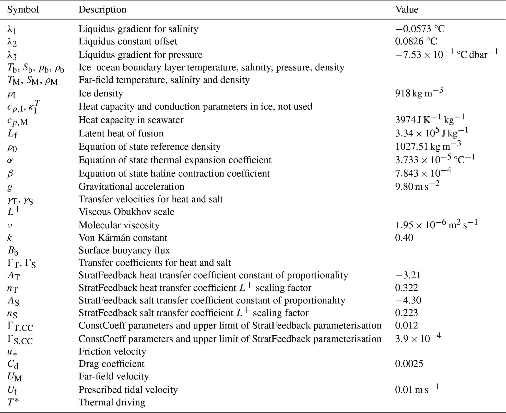
Table 1 Table of constants, variables and parameters in the basal melt parameterisations.

2.2 Stratification feedback on turbulence – insights from large eddy simulations

Stratification due to buoyant meltwater has two distinct effects on the melt rate. One is the effect of meltwater to cool and freshen the surface boundary layer, which decreases the relevance of the far-field temperature that parameterisations generally consider to be a heat source for melting (Rosevear et al., 2022b). The other is the ability of stratification to suppress boundary layer turbulence beneath horizontal or gently sloping ice shelves (noting that the same turbulence feedback may not apply beneath steeply sloped ice bases where meltwater can drive buoyant flow up-slope, generating turbulence). It is this second effect that we focus on. The stratification within Antarctic ice shelf cavities is dominated by salinity variation. Meltwater, which is relatively fresh and therefore buoyant, tends to stratify the water column.

Vreugdenhil and Taylor (2019) and Rosevear et al. (2022b) use LES beneath horizontal and weakly sloped ice bases to diagnose regimes of Antarctic ice shelf melt based on the viscous Obukhov scale L⁺, a non-dimensional variable defined as the ratio of the Obukhov length L and a viscous length scale δ_ν:

$$\begin{array}{}\text{(5)}& L^{+}={\displaystyle \frac{L}{{\mathit{\delta }}_{\mathit{\nu }}}}={\displaystyle \frac{\frac{-u_{*}^{\mathrm{3}}}{k{B}_{\mathrm{b}}}}{\mathit{\nu }/u_{*}}}={\displaystyle \frac{-u_{*}^{\mathrm{4}}}{\mathit{\nu }k{B}_{\mathrm{b}}}},\end{array}$$

where ν is the molecular viscosity, k the von Kármán constant (Table 1) and B_b the surface buoyancy flux. Assuming transfer velocities given by the three-equation melt parameterisation (Eqs. 1–4), the surface buoyancy flux can be written as

$$\begin{array}{}\text{(6)}& B_{\mathrm{b}}=-g\left(\mathit{\beta }(S_{\mathrm{M}}-S_{\mathrm{b}})u_{*}{\mathrm{\Gamma }}_{\mathrm{S}}-\mathit{\alpha }(T_{\mathrm{M}}-T_{\mathrm{b}})u_{*}{\mathrm{\Gamma }}_{\mathrm{T}}\right),\end{array}$$

with α and β the linear thermal expansion and haline contraction coefficients and g the gravitational acceleration (Table 1). We focus only on positive values of L⁺, indicating a stabilising (negative sign) buoyancy flux; the LESs do not explore freezing and destabilising conditions. Note $\mathit{\beta }/\mathit{\alpha }\sim \mathrm{20}$ °C under ice shelf cavity conditions (Asay-Davis et al., 2016), so salinity changes dominate the buoyancy flux. A small L⁺ means the flow is affected everywhere by either stratification or molecular viscosity, which both suppress turbulence. Alternatively, L⁺ can be thought of as measuring the relative importance of shear currents (represented by u_*) to buoyancy and stratification on the flow.

L⁺ can be used to distinguish regimes of ice shelf melting. Rosevear et al. (2022a) and Vreugdenhil and Taylor (2019) use LES beneath horizontal ice and find that at large $L^{+}\ge \mathcal{O}\left({\mathrm{10}}^{\mathrm{4}}\right)$, corresponding to low temperatures (small T_M−T_b) and fast flows (large u_*), the ice shelf cavity is in a well-mixed regime. In this regime, melting is controlled by velocity shear, and the transfer coefficients are similar to J10 and HJ99-M81; therefore existing parameterisations perform well (Rosevear et al., 2022a) (Fig. 1a, b). At smaller viscous Obukhov scales, $\mathcal{O}\left({\mathrm{10}}^{\mathrm{4}}\right)>L^{+}>\mathcal{O}\left({\mathrm{10}}^{\mathrm{3}}\right)$, corresponding to warmer and more quiescent flows, the ice shelf cavity enters a stratified regime where buoyant meltwater acts to suppress turbulence, but melting is still shear-driven, thus effectively decreasing the transfer coefficients. Finally, at low $L^{+}<\mathcal{O}\left({\mathrm{10}}^{\mathrm{3}}\right)$ (we use $L^{+}<\mathrm{2500}$ as the cut-off, following Rosevear et al., 2022b), corresponding to the warmest and most quiescent flows, the ice shelf cavity enters the diffusive–convective regime, where the difference between the salt and heat diffusivities results in diffusive convection, and melt rates are transient and dependent on a diffusive–convective timescale (Rosevear et al., 2022b; Middleton et al., 2021). Due to its transient nature, this regime is inherently difficult to parameterise and is not the focus of our work. Note that these ice shelf cavity regime definitions, defined by L⁺ values, differ slightly from Rosevear et al. (2022b). Here, we describe the stratified regime as the ice shelf cavity conditions where stratification suppresses turbulence. In contrast, the Rosevear et al. (2022b) stratified regime definition includes the effect of stratified meltwater to cool the boundary layer relative to the far-field temperature as mentioned earlier, which is not captured by L⁺.

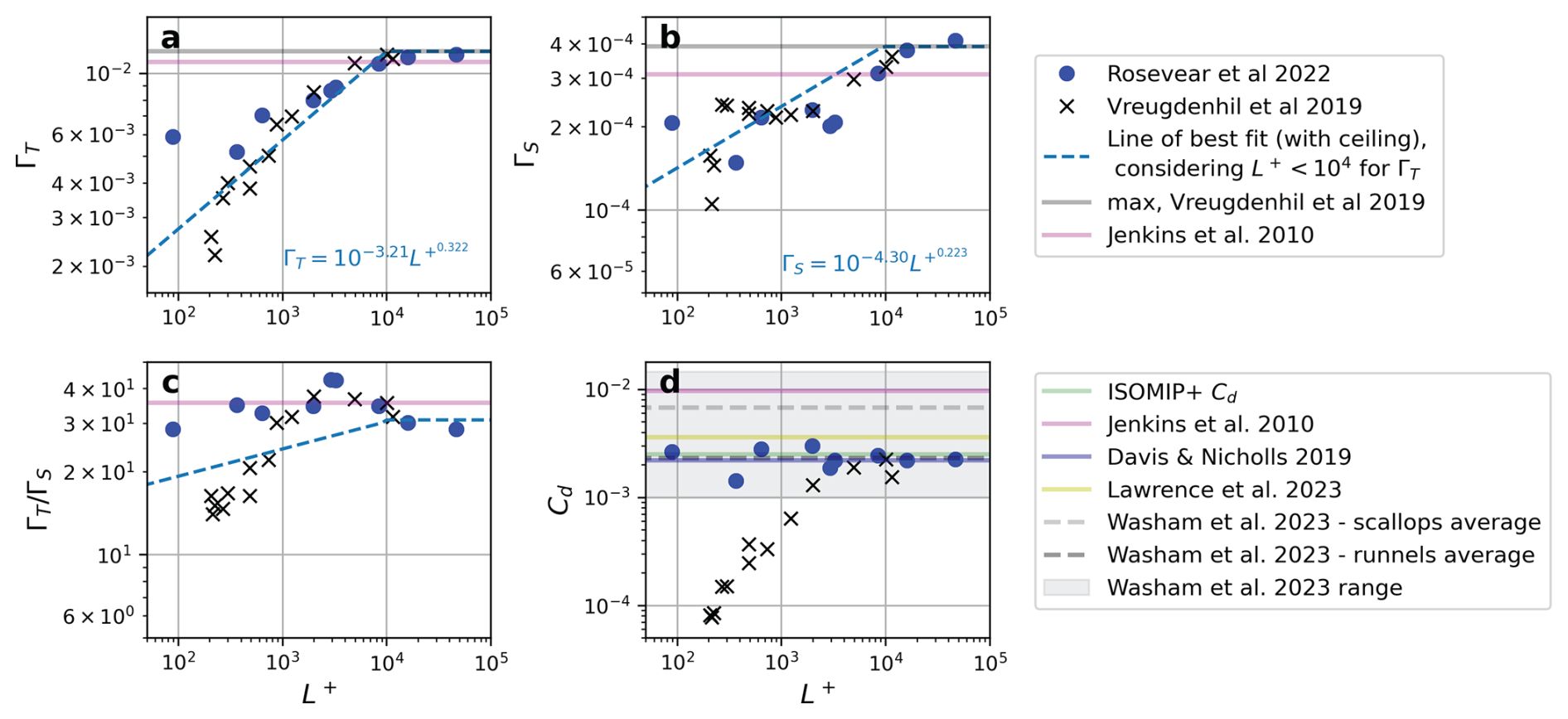
Figure 1 LES data, with Vreugdenhil and Taylor (2019) in the black crosses and Rosevear et al. (2022b) in blue dots, indicating the relationship between transfer coefficients (a) Γ_T and (b) Γ_S, their ratio (c) ${\mathrm{\Gamma }}_{\mathrm{T}}/{\mathrm{\Gamma }}_{\mathrm{S}}$, and (d) drag coefficient C_d against viscous Obhukov scale L⁺. The maximum Vreugdenhil and Taylor (2019) (ConstCoeff) values of the transfer coefficients are included (grey lines), which are similar to the Jenkins et al. (2010) values (pink lines). The dashed blue line indicates the choice of fit of transfer coefficients as a function of viscous Obukhov scale for our stratification feedback parameterisation. Drag coefficients inferred from observations of Jenkins et al. (2010), Davis and Nicholls (2019), Lawrence et al. (2023) and Washam et al. (2023) are also included.

2.3 Stratification feedback parameterisation design

The stratification feedback (StratFeedback) basal melt parameterisation explored in this study is based on the results of Rosevear et al. (2022b) and Vreugdenhil and Taylor (2019) to incorporate the unresolved suppression of turbulence by buoyant meltwater along horizontal or gently sloping ice. Both studies suggest an increase in heat and salt transfer coefficients (calculated from heat and salt gradients) with the viscous Obukhov scale up to a constant value (Fig. 1a, b). Assuming a power law relationship, we calculate a line of best fit through the log–log representation of the Γ–L⁺ data where $L^{+}<\mathrm{1}\times {\mathrm{10}}^{\mathrm{4}}$ but enforce a maximum of Γ_T and Γ_S to be the maximal limits from Vreugdenhil and Taylor (2019) (which is slightly greater than J10). The Vreugdenhil and Taylor (2019) maxima are also our “control” parameterisation with constant transfer coefficients (ConstCoeff or CC in Eq. 4). We force the line to reach these ConstCoeff parameters at $L^{+}=\mathrm{1}\times {\mathrm{10}}^{\mathrm{4}}$ so that the transition point from the well-mixed to stratified regimes is the same for both temperature and salinity, and the ratio ${\mathrm{\Gamma }}_{\mathrm{T}}/{\mathrm{\Gamma }}_{\mathrm{S}}$ is monotonic. This fit is chosen for simplicity since it is not possible to determine from the data (Fig. 1) at exactly which L⁺ the regime transitions for heat and salt transport occur. We also include data points in the diffusive–convective regime ($L^{+}<\mathrm{2500}$) since the same relationship between transfer coefficients and L⁺ tends to hold as in the stratified regime (except for $L^{+}<\mathrm{500}$), providing more data. In this way, our parameterisation intended for the stratified regime also reasonably represents melt rates for part of the diffusive–convective regime. If $L^{+}>\mathrm{0}$, the resultant StratFeedback parameterisation is

$$\begin{array}{}\text{(7)}& {\displaystyle }{\mathrm{\Gamma }}_{\mathrm{T}}=\text{min}\left\{{\mathrm{10}}^{A_{\mathrm{T}}}(L^{+}{)}^{n_{\mathrm{T}}},{\mathrm{\Gamma }}_{\mathrm{T},\mathrm{CC}}\right\},\text{(8)}& {\displaystyle }{\mathrm{\Gamma }}_{\mathrm{S}}=\text{min}\left\{{\mathrm{10}}^{A_{\mathrm{S}}}(L^{+}{)}^{n_{\mathrm{S}}},{\mathrm{\Gamma }}_{\mathrm{S},\mathrm{CC}}\right\},\end{array}$$

where the values of the constants are presented in Table 1. If $L^{+}<\mathrm{0}$, the viscous Obukhov scale and melt rate are negative, that is, the ice–ocean boundary layer is freezing. Since the LES studies we follow do not explore freezing conditions, we use the ConstCoeff (CC) transfer coefficients Γ_T,CC and Γ_S,CC when $L^{+}<\mathrm{0}$. Note that we also neglect the conductive heat flux term of Eq. (2). The conductive heat flux may be an important term under some ice shelf cavity conditions (Holland and Jenkins, 1999; Arzeno et al., 2014; Washam et al., 2020; Schmidt et al., 2023; Washam et al., 2023; Wiskandt and Jourdain, 2025), but melt rates are not expected to decrease by more than a value on the order of 10 % (Holland and Jenkins, 1999). Thus, we do not expect qualitatively different conclusions in the comparison of transfer coefficient parameterisations when we omit the conductive heat flux term. Since the transfer coefficients depend on L⁺, which in turn depends on melt rate via surface buoyancy forcing, iteration is required for convergence of the three-equation parameterisation solution. We note that other functional forms of a variable transfer coefficient would fit the data of Fig. 1a, b (e.g. Rosevear et al., 2022b consider a logarithmic fit). To briefly explore the sensitivity to our choice, we also tested steeper and shallower gradient power laws (Appendix A2).

We could also consider an alternative parameterisation where the drag coefficient, as well as the transfer coefficients, is varied. Monin–Obukhov theory expects that under a stabilising buoyancy flux, the drag coefficient is also reduced as the friction velocity is suppressed relative to a fixed far-field velocity (the drag coefficient is defined as the ratio of these speeds). Indeed, Vreugdenhil and Taylor (2019) find a reduction in the drag coefficient in LES experiments with smaller L⁺. However, Rosevear et al. (2022b) do not see a systematic variation in drag coefficient with L⁺ (Fig. 1d). The difference in the behaviour of the drag coefficients between the LES studies, which otherwise agree strongly, is likely due to the different methods of forcing the current beneath the ice. We assume the approach of Rosevear et al. (2022b), which involves forcing the model domain with a steady, far-field flow in geostrophic balance and allowing an Ekman boundary layer to form, to be somewhat more realistic. We therefore choose to follow the data of Rosevear et al. (2022b) in Fig. 1d and keep the drag coefficient constant in our study. Note that changing C_d would also change the surface boundary drag law parameterisation in some ocean models.

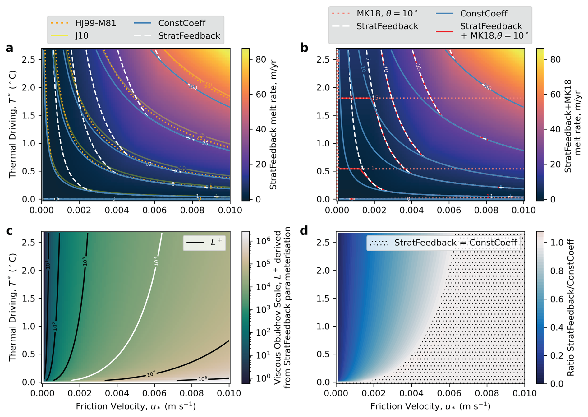
Figure 2 Thermal driving–friction velocity parameter space diagram indicating melt rates calculated as a function of far-field temperature, salinity and pressure (which are set to S=34.5 psu and p=500 dbar) and friction velocity. The melt rates are solved for a variety of parameterisation options in (a) and (b). The dotted orange lines in panel (a) are the Holland and Jenkins (1999) formulation with the η_* stratification parameter (McPhee, 1981). A constant transfer coefficient formulation (ConstCoeff) is shown by the solid blue lines (using the maximal values of Vreugdenhil and Taylor (2019), which are similar to Jenkins et al. (2010) shown by the solid light-yellow lines), and the stratification feedback (StratFeedback) parameterisation we develop here is shown by dashed white lines. In panel (b), we add in the velocity-independent melt rates obtained from McConnochie and Kerr (2018) with a slope angle of $\mathit{\theta }={\mathrm{10}}^{\circ }$ from the horizontal shown by the dotted pink line and the combination of the StratFeedback + MK18 limit shown by the dash-dot red line. Panel (c) shows the viscous Obukhov scale L⁺ derived from the stratification feedback parameterisation. The white $L^{+}=\mathrm{1}\times {\mathrm{10}}^{\mathrm{4}}$ indicates where the dashed white lines (StratFeedback) and the blue line (ConstCoeff) transition from having the same melt rate to the right and a different melt rate to the left. Panel (d) also shows this with the ratio of the StratFeedback to ConstCoeff melt rates, with stippling indicating where they are equal.

To illustrate the effect of the StratFeedback parameterisation, we solve the three-equation parameterisation (Eqs. 1–3) with several transfer coefficient parameterisations across different ice shelf cavity regimes. We vary the far-field temperature T_M and friction velocity u_* and compute melt rates across this parameter space with the StratFeedback, ConstCoeff, J10 and HJ99-M81 transfer coefficients, assuming S_M=34.5 psu and a pressure p_b of 500 dbar (∼ 500 m depth). Rather than plot the far-field temperature on the y axis, we instead plot the corresponding thermal driving,

$$\begin{array}{}\text{(9)}& T^{*}=T_{\mathrm{M}}-T_{\mathrm{fr}}\left(S_{\mathrm{M}}\right),\end{array}$$

which quantifies the maximum heat available for melting (where $T_{\mathrm{fr}}\left(S\right)={\mathit{\lambda }}_{\mathrm{1}}S+{\mathit{\lambda }}_{\mathrm{2}}+{\mathit{\lambda }}_{\mathrm{3}}{p}_{\mathrm{b}}$ is the local freezing point as in Eq. 1). Note this thermal driving is larger than the actual temperature difference between the far-field ocean and ice–ocean interface, which is computed using the three-equation parameterisation (T_M−T_b in Eq. 2), as observed under stratified conditions (Schmidt et al., 2023; Washam et al., 2023). However, this thermal driving definition is independent of transfer coefficient parameterisations and therefore more appropriate when comparing parameterisations.

Figure 2a demonstrates that the ConstCoeff, J10 and HJ99-M81 transfer coefficients have similar melt rate contours in the thermal driving–friction velocity parameter space. The ratio of HJ99-M81 and ConstCoeff is relatively uniform except at very low velocities, where the McPhee (1981) stability parameter becomes relevant (Fig. A1c; and recall that many ocean models set ${\mathit{\eta }}_{*}=\mathrm{1}$ for simplicity and therefore do not account for this stratification parameter. Melt rates under this “HJ99-neutral” parameterisation are greater than HJ99-M81; see Fig. A1b). However, the magnitude of the ratio to ConstCoeff is closer to 1 than for the StratFeedback parameterisation, indicating that the McPhee (1981) η_* term does not capture the full extent of the stratification feedback on melt seen in the LES studies. StratFeedback limits to ConstCoeff at high friction velocities and lower thermal driving ($L^{+}>{\mathrm{10}}^{\mathrm{4}}$; Fig. 2c) but changes gradient and has relatively less melting in warmer and more quiescent conditions (the diffusive–convective and stratified regimes), also indicated by the melt rate ratio (Fig. 2d). At a thermal driving of $T^{*}=\mathrm{2}$ °C and $u_{*}=\mathrm{0.001}$ m s⁻¹ (far-field velocities of ∼2 cm s⁻¹, on the lower end of observed speeds; Table B1), StratFeedback predicts 30 % of the ConstCoeff melt, indicating that the StratFeedback parameterisation significantly modifies melt rates in some ice shelf cavity regimes. Figure 2b uses alternative parameterisation choices in this low-velocity regime that are explained in Sect. 2.5.

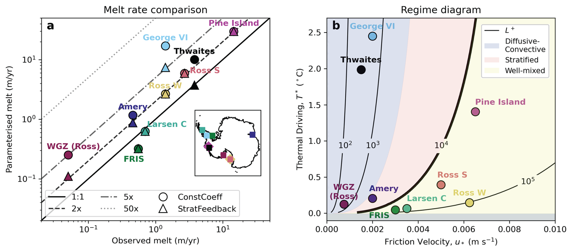
Figure 3 Parameterised melt against observed melt rate (a) for borehole observational data updated from Rosevear et al. (2022a), with the ConstCoeff parameterisation in circles and StratFeedback in triangles. Thermal driving T^* (Eq. 9)–friction velocity regime (b) updated from Rosevear et al. (2022b), where the thick L⁺ line of 1×10⁴ divides where the StratFeedback parameterisation diverges (to the left) and where the transfer coefficients are constant and equal to ConstCoeff (to the right). The diffusive–convective ($L^{+}<\mathrm{2500}$), stratified ($\mathrm{2500}<L^{+}<{\mathrm{10}}^{\mathrm{4}}$) and well-mixed–shear-driven ($L^{+}>{\mathrm{10}}^{\mathrm{4}}$) regimes are shaded. Data are obtained from the Filchner–Ronne Ice Shelf (FRIS; Jenkins et al., 2010), Larsen C Ice Shelf (Davis and Nicholls, 2019), Amery Ice Shelf (Rosevear et al., 2022a), Ross Ice Shelf (Ross S for summer and Ross W for winter data; Stewart, 2018), WISSARD grounding zone of the Ross Ice Shelf (WGZ (Ross); Begeman et al., 2018), George VI Ice Shelf (Kimura et al., 2015; Middleton et al., 2022), Pine Island Glacier (Stanton et al., 2013) and Thwaites Glacier (Davis et al., 2023). Further computation details are supplied in Table B1.

2.4 Comparison with observations

Following Rosevear et al. (2022a), we compare the melt rate produced by the StratFeedback and ConstCoeff three-equation melt parameterisations using limited direct observations of borehole ocean conditions and co-located, direct melt rate measurements in Antarctic ice shelves (Fig. 3; data presented in Appendix B). If the parameterisations accurately predicted melt from temperature, salinity, pressure and velocity observations, we would expect the points to lie on the solid 1:1 line of Fig. 3a. However, we find that in general, the ConstCoeff parameterisation overestimates the melt, except for at the Larsen C Ice Shelf and Filchner–Ronne Ice Shelf (FRIS). Note that the studies that originally presented this data may have used slightly different melt parameterisations in their comparisons (e.g. Jenkins et al., 2010; Davis and Nicholls, 2019, where different drag coefficients and transfer coefficients were used), and recall that we ignore heat conduction into the ice. Additionally, the studies may use different thermodynamic variables. Here we use conservative temperature and absolute salinity with conversions performed using the Gibbs Seawater Oceanographic Toolbox (McDougall and Barker, 2011, Appendix B). However, these choices are not expected to qualitatively change the overestimation of melt rates. The original studies may also classify their ice shelf regimes differently; for example, Davis et al. (2023) categorise their observed Thwaites Ice Shelf conditions as stratified turbulence, whereas our definitions place it in the diffusive–convective regime (Fig. 3).

For five of the ice shelf borehole locations, the melt rate does not change between the ConstCoeff and StratFeedback parameterisations (Fig. 3a, co-located circles and triangles). This is because the viscous Obukhov scale L⁺ is greater than 1×10⁴, indicating these ice shelves are in the well-mixed melt regime (Fig. 3b). However, several of these high-L⁺ locations still have overestimated parameterised melt by a factor of ∼2 for both the ConstCoeff and StratFeedback parameterisations. A likely explanation is a second impact of stratification on melt rate: even under high-L⁺ conditions, the development of a cold meltwater layer can decrease the thermal driving relative to that expected by the far-field temperature, which our StratFeedback parameterisation does not address. However, parameterised melt rates decrease when using the StratFeedback rather than ConstCoeff parameterisation for the borehole observations at Amery, George VI and Thwaites ice shelves and the grounding zone of the Ross Ice Shelf (WGZ) (Fig. 3a, triangles lower than circles; therefore parameterised melt is closer to matching observed melt rates at the 1:1 line). Of these locations, George VI, Thwaites and WGZ have small L⁺ (Fig. 3b), suggesting they may be in the diffusive–convective melt regime and that the StratFeedback parameterisation is still missing physics for these ice shelves. We discuss a possible approach for bridging the transition between stratified and diffusive–convective regimes in Sect. 2.5. Nevertheless, the improvement in overestimation of melt rates for the ice shelves in the stratified regime, such as Amery Ice Shelf (as well as the benefit seen in the diffusive–convective regime), motivates us to implement and test the StratFeedback parameterisation in ocean models.

2.5 Limiting to a velocity-independent parameterisation

There are both numerical and physical reasons for the low-velocity ice shelf cavity regime to be specially treated with the three-equation parameterisation. The low-velocity regime is characterised by low velocities, here taken as far-field flows of 1 cm s⁻¹ or smaller, but has considerable overlap with the $L^{+}<\mathrm{2500}$ diffusive–convective regime. Numerically, a friction velocity of zero (perhaps created by initialising the model at rest) will result in identically zero melt according to Eqs. (2)–(4), which would be inconsistent with the presence of heat available for melting and may also lead to numerical problems while solving for the melt rate. Physically, in the diffusive–convective regime with $L^{+}<\mathcal{O}\left({\mathrm{10}}^{\mathrm{3}}\right)$, the StratFeedback parameterisation is an extrapolation. When the friction velocity is $\mathrm{5}\times {\mathrm{10}}^{-\mathrm{4}}$ m s⁻¹, Fig. 2d shows that the StratFeedback parameterisation can have 10 times less melt than the ConstCoeff formulation. Indeed, at very low velocities the melt rate with the stratification feedback could become arbitrarily small, when in reality we always expect some melt in the presence of a thermal or haline driving even without far-field currents, as a result of the effect of diffusive convection beneath horizontal ice (Rosevear et al., 2021; Middleton et al., 2021) or buoyant convection beneath sloping ice (McConnochie and Kerr, 2018; Mondal et al., 2019).

To address this limit, we also implement a transition from the shear-driven parameterisation to a convective, free-stream velocity-independent parameterisation based on laboratory studies of sloped ice (McConnochie and Kerr, 2018, hereafter MK18) and similar direct numerical simulations (Mondal et al., 2019). Velocity-independent refers to the velocity of the free-stream flow as captured by the ocean model, which does not appear in the convective melt equations. We note, however, that melting of a sloping ice face produces a buoyant plume with its own velocity, which is implicitly included in the convective parameterisation. Similarly to the methods of Schulz et al. (2022) and Zhao et al. (2024) for vertical ice melt parameterisations, we transition to alternative transfer velocities for heat and salt at low velocities. The effective transfer velocities are determined by the slope of the ice base, θ from the horizontal, and other thermodynamic variables (derivation in Appendix A3):

$$\begin{array}{}\text{(10)}& {\displaystyle }\begin{array}{rl}{\mathit{\gamma }}_{\mathrm{T},\mathrm{eff}}=& \mathit{\chi }{\sin }^{\mathrm{2}/\mathrm{3}}\mathit{\theta }\\ & {\left({\displaystyle \frac{g\left(\mathit{\beta }\left(S_{\mathrm{M}}-S_{\mathrm{b}}\right)-\mathit{\alpha }\left(T_{\mathrm{M}}-T_{\mathrm{b}}\right)\right)}{\mathit{\nu }}}\right)}^{\mathrm{1}/\mathrm{3}}\\ & {\mathit{\kappa }}_{\mathrm{s}}^{\mathrm{1}/\mathrm{6}}{\mathit{\kappa }}_{\mathrm{T}}^{\mathrm{1}/\mathrm{2}},\end{array}\text{(11)}& {\displaystyle }{\mathit{\gamma }}_{\mathrm{S},\mathrm{eff}}={\mathit{\gamma }}_{\mathrm{T},\mathrm{eff}}{\displaystyle \frac{{\mathit{\rho }}_{\mathrm{I}}{S}_{\mathrm{b}}}{{\mathit{\rho }}_{\mathrm{0}}{S}_{\mathrm{M}}}}\sqrt{{\displaystyle \frac{{\mathit{\kappa }}_{\mathrm{S}}}{{\mathit{\kappa }}_{\mathrm{T}}}}},\end{array}$$

with χ an experimentally derived non-dimensional constant and other parameters defined in Appendix A3 and Table A1. We choose to transition between regimes by computing the maximum of the velocity-dependent (Eq. 4) and MK18 velocity-independent transfer velocities (Fig. 2b; red line connects the dashed white line, the StratFeedback shear-driven parameterisation, and the dotted orange line, the MK18 limit at a given ice base angle of 10°, a value within the limits of those observed by Wåhlin et al., 2024, though equivalent plots with different angles are provided in Fig. A2). That is,

$$\begin{array}{}\text{(12)}& {\displaystyle }{\mathit{\gamma }}_{\mathrm{T}}=\text{max}\left({\mathrm{\Gamma }}_T{u}_{*},{\mathit{\gamma }}_{\mathrm{T},\mathrm{eff}}\right),\text{(13)}& {\displaystyle }{\mathit{\gamma }}_{\mathrm{S}}=\text{max}\left({\mathrm{\Gamma }}_S{u}_{*},{\mathit{\gamma }}_{\mathrm{S},\mathrm{eff}}\right).\end{array}$$

Therefore, at low velocities, the melt rate is independent of far-field velocity U_M. This formulation differs from McConnochie and Kerr (2017), who propose a transition between shear-driven and convective melt regimes at a critical velocity, noting that the transition conditions are still poorly constrained (Rosevear et al., 2025). The dependence on ice base slope means that beneath horizontal ice shelves (θ=0°) the MK18 melt rate will still be zero. MK18 and Mondal et al. (2019) do not recommend using this parameterisation on gently sloped ice with angles less than 2°; therefore, the MK18 limit applied to gently sloped Antarctic ice shelves is still an extrapolation into a poorly explored ice shelf regime. Additionally, local slope calculations are horizontal-resolution-dependent. Alternative formulations not explored here could account for the melting of unresolved steeper slopes using an enhancement factor based on the expected distribution of small-scale features.

We also explore other alternatives for a velocity-independent parameterisation under quiescent conditions: a minimum friction velocity and a prescribed tidal velocity, created by altering the definition of the friction velocity. The minimum friction velocity method is expressed as

$$\begin{array}{}\text{(14)}& u_{*}=max\left\{C_{\mathrm{d}}^{\mathrm{1}/\mathrm{2}}{U}_{\mathrm{M}},u_{*,\text{min}}\right\},\end{array}$$

where the minimum velocity is intended to represent heat transport occurring through molecular diffusion even at very low current speeds (Gwyther et al., 2016). Using a minimum velocity is a simplification for models that do not resolve the boundary layer, and this velocity does not account for the true viscous sublayer thermodynamics. Alternatively, one could consider unresolved, high-frequency tidal velocities that increase the mean friction velocity. The ISOMIP+ (Asay-Davis et al., 2016) protocol calculates friction velocity by adding a tidal velocity U_t in quadrature with the far-field velocity U_M, scaled by the square root of the drag coefficient:

$$\begin{array}{}\text{(15)}& u_{*}=C_{\mathrm{d}}^{\mathrm{1}/\mathrm{2}}\sqrt{U_{\mathrm{M}}^{\mathrm{2}}+U_{\mathrm{t}}^{\mathrm{2}}}.\end{array}$$

This formulation also enforces a minimum friction velocity.

The different transfer coefficient parameterisations and low-velocity limits used in the three-equation basal melt parameterisations that are discussed in this study are summarised in Table 2. Each choice of transfer and drag coefficient can be combined with each choice of low-velocity limit. In particular, the StratFeedback + MK18 parameterisation is intended to best represent real ice shelf–ocean regimes, since it encompasses the commonly used shear-driven melt parameterisation under well-mixed, shear-driven conditions, the stratified suppression of turbulence observed and suggested by LESs, and a lab-based velocity-independent convective parameterisation when far-field flows are weak. In this study, we assess the sensitivity to the choice of low-velocity limits with the transfer coefficient parameterisation choices, ConstCoeff and StratFeedback.

Jenkins et al. (2010)Holland and Jenkins (1999)McPhee (1981)Holland and Jenkins (1999)Vreugdenhil and Taylor (2019)Vreugdenhil and Taylor (2019)Rosevear et al. (2022b)Asay-Davis et al. (2016)McConnochie and Kerr (2018)Mondal et al. (2019)Adusumilli et al. (2020a)

Table 2 Summary of three-equation basal melt parameterisation transfer coefficients Γ_T and Γ_S used in this study. The five transfer coefficient parameterisations assume a friction velocity calculated from the drag coefficient C_d. When implemented in the idealised models, we also explore alternative low-velocity limit choices combined with the ConstCoeff and StratFeedback transfer coefficients, which modify the parameterisation at low friction velocities. The tuned Pine Island Glacier simulation method is explained in Sect. 3.2.

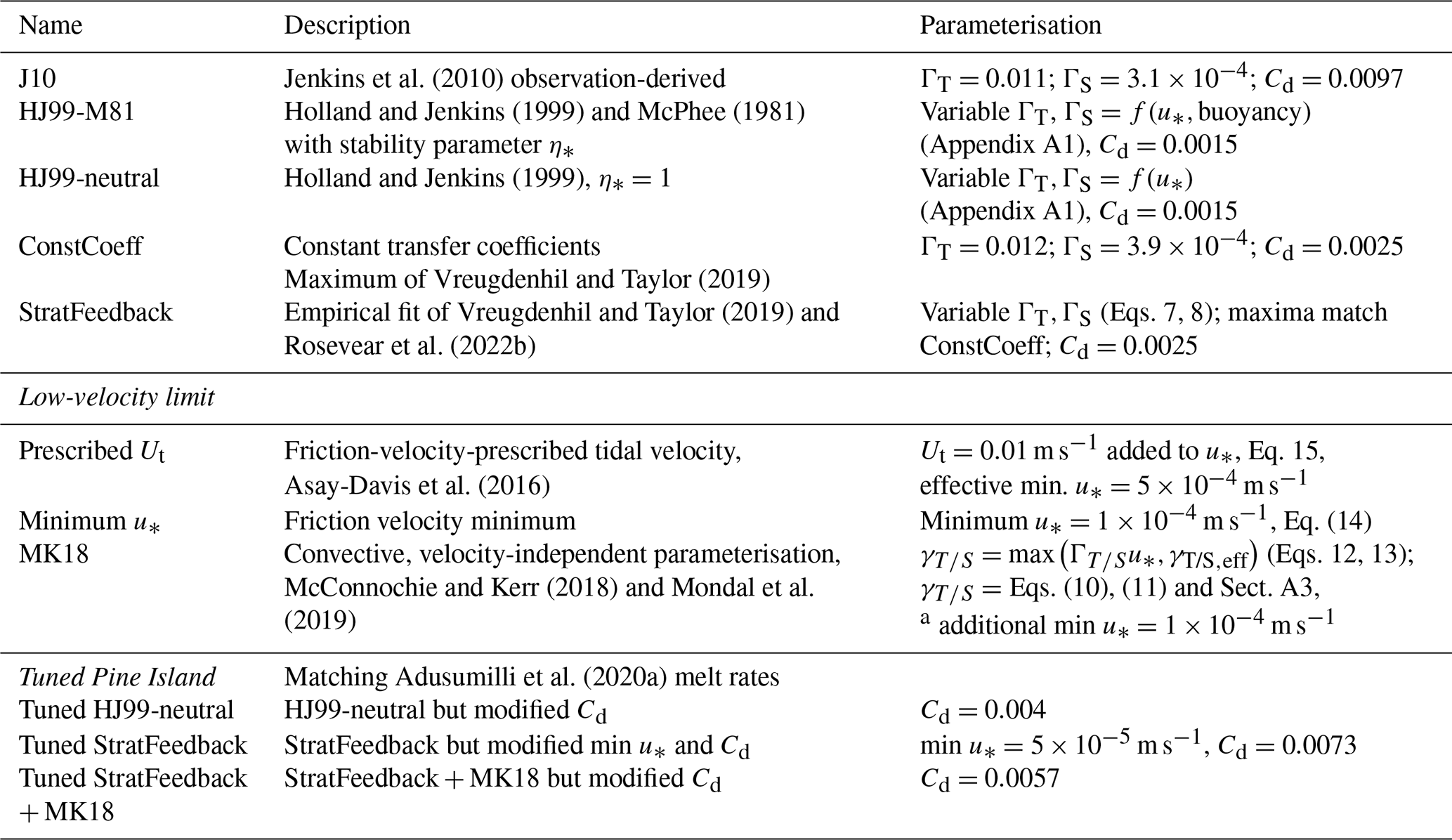
^a Required for numerical stability to avoid zero transfer velocities in the case of horizontal slopes (0°) and no flow, with little effect on the results as the MK18 effective transfer velocities are generally larger than ${\mathrm{\Gamma }}_{\text{T,S}}{u}_{*,\text{min}}$, except when θ<0.05°, and $u_{*}<\mathrm{1}\times {\mathrm{10}}^{-\mathrm{4}}$ m s⁻¹.

3 Model configurations

To test the performance of the stratification feedback parameterisation in a three-dimensional ice-shelf-cavity-scale model, we implement the parameterisation in two widely used ocean models, MOM6 and MITgcm. We use the Second Ice Shelf-Ocean Model Intercomparison Project (ISOMIP+) configuration (Asay-Davis et al., 2016) to assess the effect of the parameterisation in an idealised configuration. Then, to explore different regimes of Antarctic ice shelf cavities, the MOM6 ISOMIP+ experiments are modified to include idealised barotropic tides of varying amplitude. Finally, the parameterisation is tested in a high-resolution simulation of Pine Island Glacier (Nakayama et al., 2021) in the Amundsen Sea. In this section, we briefly describe the ISOMIP+ experiment (and refer the reader to Asay-Davis et al., 2016, for further details) followed by each of the ocean models used in this study.

3.1 ISOMIP+ setup and modifications

We use the idealised ISOMIP+ Ocean0 model configuration (Asay-Davis et al., 2016) in both MOM6 and MITgcm, which are also submissions to the ISOMIP+ intercomparison project (Yung et al., 2025a). The Ocean0 ice shelf draft and bathymetry represent an idealised ice shelf cavity with walls at either side and a grounding line. To assess different regimes of ice shelf cavities, we use both the warm and cold ISOMIP+ potential temperature and salinity distributions as initial conditions and restoring boundary forcing, all linear as a function of depth. In this way, our warm test case is effectively the Ocean0 experiment of ISOMIP+, and our cold test case is a static, cold version of Ocean1, also used in Gwyther et al. (2020). The warm configuration has a temperature of 1 °C and salinity of 34.55 psu at the bottom of the cavity, aiming to simulate the presence of warm water intrusions, varying linearly to −1.9 °C and 33.8 psu at the surface. The cold configuration has a spatially uniform temperature of −1.9 °C and a salinity range of 33.8 to 34.7 psu. The salinity, temperature and layer interfaces are restored at the northern boundary using a sponge with a restoring timescale of 0.1 d. Note these temperature and salinity profiles are highly idealised, and the cold configuration is unrealistically fresh compared to the conditions within and outside the Ross and Weddell Sea ice shelves (Orsi and Wiederwohl, 2009; Nicholls et al., 2004; Darelius et al., 2014). We use 36 vertical layers, though we note the difference in vertical coordinates between MOM6 and MITgcm described below. Unless specified, we follow the mixing, viscosity and equation of state protocols of ISOMIP+ (Asay-Davis et al., 2016). This protocol includes the f-plane approximation with a latitude of 75° S.

To simulate basal melt, we use the three-equation parameterisation (Eqs. 1–3) without the ice heat conduction term (noting melt rates would decrease by ∼ 10 % if this term were to be included). We perform experiments with the StratFeedback and ConstCoeff transfer coefficients and each of the three low-velocity limit choices (Sect. 2; summarised in Table 2). In all ISOMIP+ simulations, the drag coefficient C_d=0.0025 is used for the melt parameterisation and top and bottom boundary conditions for momentum, consistent with Asay-Davis et al. (2016) and Gwyther et al. (2020).

All idealised experiments are run for 730 d. By this time, models are spun up to an equilibrium state.

3.1.1 Idealised MOM6 configuration

The Modular Ocean Model 6 (MOM6; Adcroft et al., 2019) is a finite-volume, hydrostatic ocean model which has been used for idealised simulations of ice shelf cavities (Stern et al., 2019). MOM6 is configured on an Arakawa C grid with a generalised vertical coordinate, though here we employ the isopycnal layered version of the model rather than its Arbitrary Lagrangian–Eulerian vertical coordinate capabilities (Griffies et al., 2020). We use a Kraus and Turner (1967)- and Niiler and Kraus (1977)-like bulk mixed layer parameterisation for the surface boundary layer (Hallberg, 2003), which energetically constrains the boundary layer depth, and the Jackson et al. (2008) vertical mixing parameterisation with a critical Richardson number of 0.25.

The MOM6 ice shelf thermodynamics code numerically solves the three-equation parameterisation using an iterative loop, and both a constant transfer coefficient (e.g. Jenkins et al., 2010) and the variable formulation (Holland and Jenkins, 1999; McPhee et al., 1987) can be used. The new stratification feedback parameterisation is implemented with an additional iterative loop to solve for the melt rate, buoyancy forcing and viscous Obukhov scale as described in Sect. 2. The model samples temperature, salinity and velocity over the bulk mixed layer (approximately 10 m thick) in the melt parameterisation, then inserts freshwater in the bulk mixed layer as a volume flux (which can later be entrained in the interior ocean layers; Hallberg, 2003). The magnitude of melting is likely to be sensitive to these choices, as well as to the vertical resolution (Gwyther et al., 2020). Melting is set to zero when the ocean column is less than 10 m thick. The friction velocity u_* is calculated from the velocities in the uppermost model layer (the top half of the bulk mixed layer, approximately 5 m thick). This vertical resolution is insufficient to resolve the structure of the ice shelf–ocean boundary layer, though the uppermost layers exhibit cooling and freshening in response to melting.

3.1.2 Idealised MITgcm configuration

The Massachusetts Institute of Technology general circulation model (MITgcm; Marshall et al., 1997) is a finite-volume ocean model that can simulate ice shelf cavities (Losch, 2008). MITgcm uses z (depth) coordinates and is built on an Arakawa C grid. Partial cells are included, with a minimum thickness of 25 % of the normal cell thickness of 20 m. Melt rate is calculated using a quadratic equation (Losch, 2008). Therefore, we implement an additional iterative loop that solves the three-equation system with the modified and varying transfer coefficients until the solution converges. Tracers and the velocities for the friction velocity and melt parameterisation are sampled over the uppermost 20 m layer (Losch, 2008), which generally covers more than one vertical grid cell. Meltwater is represented as a virtual salt flux rather than a volume flux, distributed over the same 20 m layer. As in MOM6, this vertical resolution is insufficient to resolve the structure of the ice shelf–ocean boundary layer. Unstable vertical mixing is parameterised with a convection scheme (Cessi and Young, 1996).

3.1.3 Idealised explicit tidal forcing

In addition to the ISOMIP+ experiments, we run an additional MOM6 case where we add an idealised barotropic tide as an open boundary condition to inject more kinetic energy into the otherwise relatively quiescent cavity. This method differs from the prescribed tidal forcing in the melt parameterisation, where the effect of tides is artificially added to the friction velocity (Sect. 2.5). By forcing tides explicitly, we capture the direct effect of tides on melting and also the indirect effects due to tidal advection, mixing and residual circulation within the cavity. Here, the sponge boundary is replaced by a Flather–Orlanski (Flather, 1976; Orlanski, 1976) open boundary, nudged to the values of the sponge configuration output, with an additional sinusoidal tidal velocity and sea surface height forcing at the M2 frequency of two cycles per 24 h and 50 min. Since the ISOMIP+ simulations are on an f plane with latitude 75° S (Asay-Davis et al., 2016), the whole domain is effectively south of the M2 critical latitude (Makinson et al., 2006). The amplitude of the tidal velocity and sea surface height are calculated by considering the volume change within the cavity as a result of the tides (with an assumption of linearity, as MOM6 permits grounding line movement), with velocity amplitudes of 0.2, 0.1, 0.05 and 0.01 m s⁻¹ matching sea surface height amplitudes at the boundary of 6.4, 3.2, 1.6 and 0.32 m, respectively. However, the resulting tidal velocity at the ice–ocean interface is lower near the grounding line compared to the ice front (Fig. S1), as seen in other modelling studies (Mueller et al., 2012; Gwyther et al., 2016; Jourdain et al., 2019). Note we use the minimum friction velocity limit of $u_{*}=\mathrm{1}\times {\mathrm{10}}^{-\mathrm{4}}$ m s⁻¹ discussed in Sect. 2.5 for numerical stability.

3.2 Pine Island Glacier configuration

For our realistic test, we use the Nakayama et al. (2021) MITgcm Pine Island Glacier configuration. This model configuration uses MITgcm with the hydrostatic approximation and has a high spatial resolution of 200 m in the horizontal and 10 m in the vertical, and has been evaluated against satellite observations (Shean et al., 2019; Adusumilli et al., 2020a) to have a realistic representation of melt (Nakayama et al., 2019). Although the model can include subglacial discharge, it is used here without this additional flux, noting that the changes in melt rate seen by adding realistic subglacial discharge are modest compared with that expected by adding the StratFeedback parameterisation (Nakayama et al., 2021). However, subglacial discharge could modify the ice shelf–ocean boundary layer, thereby altering the effect of the StratFeedback parameterisation. Dynamic and thermodynamic sea ice is included (Losch et al., 2010). The density equation of state is from Jackett and Mcdougall (1995), and the same linear freezing point equation of state as ISOMIP+ is used.

The ocean bathymetry and static ice draft are based on BedMachine-Antarctica (Morlighem et al., 2020). Tides are not included. The model is forced at the boundaries by the bias-corrected version of Nakayama et al. (2019) model output, which is in turn forced by a regional downscaling of ECCO LLC270 (Nakayama et al., 2018).

Nakayama et al. (2021) use the Holland and Jenkins (1999) velocity-dependent parameterisation with transfer coefficients dependent on the Prandtl and Schmidt numbers but where the McPhee (1981) η_* stability parameter is set to 1, and a drag coefficient C_d=0.0015 is used (i.e. the MITgcm default values and parameterisation; Losch, 2008; named HJ99-neutral in Table 2). Here, we modify the drag coefficient to achieve a tuned melt rate that matches the Adusumilli et al. (2020a) satellite-derived melt rate. We only consider latitudes south of 74.8°S due to large disagreement between models and observations in the northern region of the ice shelf (see Sect. 4.4), yielding an average melt rate of 15.1 m yr⁻¹. When tuning the MITgcm results, we mask out regions of the simulated ice shelf where Adusumilli et al. (2020a) data are unavailable (Fig. D1b). To compare the spatial distributions of melt rates for the StratFeedback and StratFeedback + MK18 parameterisations, we perform a similar tuning, requiring different drag coefficients for each parameterisation (Table 2). We run the Pine Island simulation for 50 d, starting from 30 January 2010 conditions, for each basal melt parameterisation.

4 Results

4.1 Idealised ISOMIP+ results

We compare the effect of the stratification feedback (StratFeedback) parameterisation against the more commonly used constant transfer coefficient (ConstCoeff) method using the ISOMIP+ Ocean0 warm and cold experiments in both MOM6 and MITgcm (the latter's results are presented in Appendix C). In this first section, we follow the ISOMIP+ protocol and use the low-velocity limit with a prescribed tidal contribution of U_t=0.01 m s⁻¹ to the friction velocity (Table 2). Here, the simulations do not include explicit tides. The StratFeedback parameterisation greatly affects the melt rate, boundary layer temperature, and salinity and circulation within the idealised MOM6 ice shelf cavity. Figure 4a–d demonstrate that the temperature stratification is markedly different in the warm experiments compared with the cold experiments. All simulations have lower temperatures near the ice–ocean boundary layer due to the presence of cold meltwater, but this layer is less visible in the StratFeedback experiments. The salinity stratification, which dominates the density, is similar between warm and cold experiments, with a fresh meltwater layer most prominent in the warm ConstCoeff simulation (thin blue layer at the surface of Fig. 4e), though the warm experiment has saltier deep water following the ISOMIP+ protocol. Melt rates are significantly greater in the MOM6 experiments with constant transfer coefficients compared with the same experiments using the StratFeedback parameterisation (note the different colourmap axes between the warm and cold simulations; Fig. 4i–l). Indeed, the warm experiment with the StratFeedback parameterisation (Fig. 4j) has melt rates more similar to the cold experiments (Fig. 4k–l) than its warm, constant-coefficient counterpart (Fig. 4i). Comparing MOM6 and MITgcm (see Fig. C1), we see that MITgcm has similar temperature and salinity profiles, though thicker cold, fresh meltwater layers and larger melt rates, particularly in the warm experiments, which have approximately twice the melt of MOM6 (Fig. C1; compare also centre columns in Fig. 5). Stronger melting may be associated with the z-level coordinates in MITgcm versus the higher-resolution-layer coordinate below the ice shelf in MOM6 and the different choices of thermal driving sampling depth (Gwyther et al., 2020).

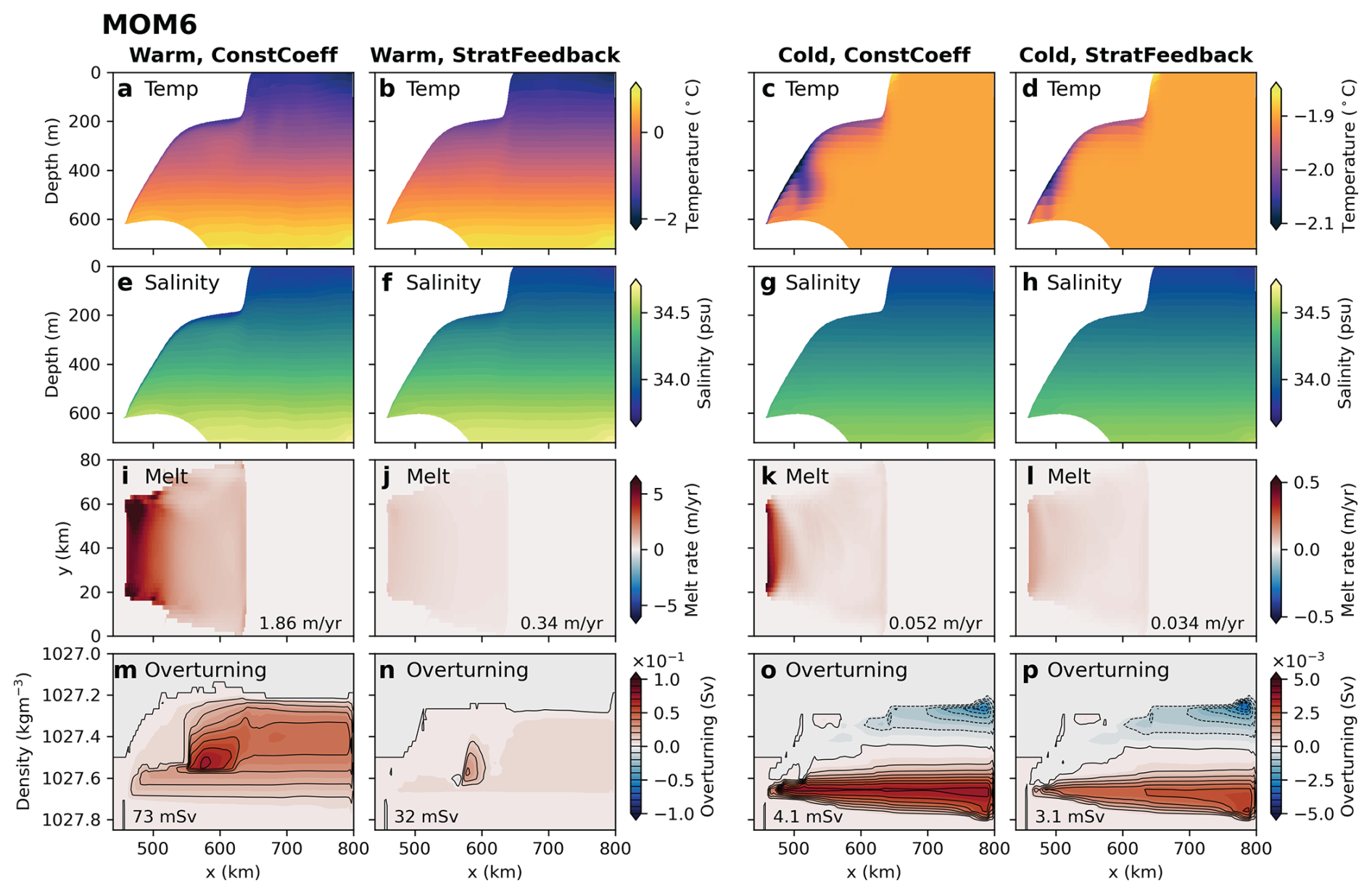
Figure 4 Temperature (a–d) and salinity (e–h) transects, melt rate distribution (i–l), and zonally averaged overturning streamfunction in density coordinates (m–p) for MOM6 simulations. All experiments use the ISOMIP+ protocol-specified tidal velocity U_t=0.01 m s⁻¹ as the low-velocity limit in the melt rate parameterisation. Variables are averaged over the last 180 d of the simulation, with the temperature and salinity profiles taken at the y=40 km transect. Warm experiments are in columns 1 and 2, cold in 3 and 4. Columns 1 and 3 show the constant-coefficient melt parameterisation results, and columns 2 and 4 contain the stratification feedback parameterisation. Melt rates averaged over the ice shelf are listed in panels (i)–(l). Black contours in (m)–(p) are spaced by 10 mSv (m–n) and 0.5 mSv (o–p), and the text lists the maximum value of the overturning streamfunction in the domain. Note the different colourbar ranges between the warm and cold simulations. Equivalent results for MITgcm are in Appendix C.

The strong reduction in melt when the StratFeedback parameterisation is included corresponds to the design of the parameterisation, which suppresses the transfer coefficients in response to a low viscous Obukhov scale, L⁺ (Sect. 2.2). L⁺ is smaller in the warm experiments due to greater thermal driving; therefore the transfer coefficients are more reduced in the warm experiments than the cold. This explains why the decrease in melt rate from the constant transfer coefficient experiments to the StratFeedback parameterisation experiments is far greater for the warm experiments than the cold, where L⁺ is larger. Still, L⁺ is not large enough in the cold experiments for the cavity to be entirely in the shear-driven regime, where $L^{+}>\mathrm{1}\times {\mathrm{10}}^{\mathrm{4}}$; otherwise, the parameterisations would have identical melt rates.

The melt rate reduction due to the stratification feedback leads to a change in ice shelf cavity circulation. Figure 4m–p shows the MOM6 overturning streamfunction (calculated in density space, where streamlines indicate the overturning circulation). In all experiments, there is an overturning circulation with buoyant water travelling up the ice–ocean boundary. In the cold experiments, there is an opposing overturning cell at lower densities, created by the conservation of volume as the lower overturning water reaches its neutral density and flows toward the boundary at x=800 km. There is a clear relationship between the magnitude of the melt rates in Fig. 4i–l and the magnitude of the overturning circulation (m–p), which are both weaker in the cold experiments than the warm (note the different colourbar scales) and weaker in the StratFeedback parameterisation experiments compared with the constant-coefficient experiments. This relationship is expected, since buoyant meltwater is the main driver of cavity circulation, which positively feeds back on melting by increasing current speeds (e.g. Holland et al., 2008; Jourdain et al., 2017).

MITgcm simulations see the same reduction in melt rate and circulation with the StratFeedback parameterisation (Fig. C1) as MOM6. Additionally, the overturning circulation is greater in MITgcm than in MOM6 for most experiments (Fig. 4 vs. Fig. C1). This can be explained by greater melt rates and therefore a stronger buoyant meltwater flow. Model choices thus affect both the magnitude of melt and the resultant ice shelf cavity circulation.

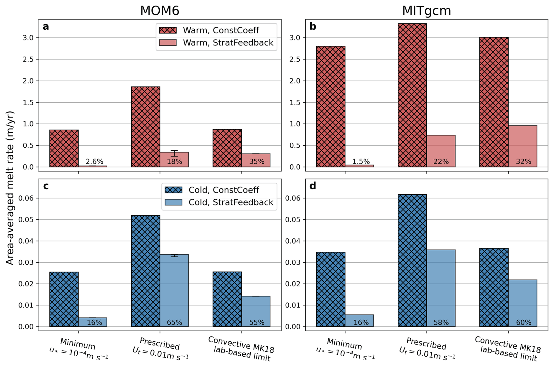
Figure 5 Area-averaged melt rates in the final 180 d of the ISOMIP+ simulations for MOM6 (a, c) and MITgcm (b, d). Warm experiments are in the top row, and cold experiments are in the bottom. Hatched bars are experiments with a constant transfer coefficient, solid colours are with the stratification feedback parameterisation, and percentages indicate the ratios of the StratFeedback to ConstCoeff melt rates. Each of the three columns within panels show the results for different choices of low-velocity limit, either a minimum friction velocity of $u_{*,\min }={\mathrm{10}}^{-\mathrm{4}}$ m s⁻¹, a prescribed tidal velocity of U_t=0.01 m s⁻¹ (which implies a minimum friction velocity of $u_{*,\min }=\mathrm{5}\times {\mathrm{10}}^{-\mathrm{4}}$ m s⁻¹) or a smooth transition to the McConnochie and Kerr (2018) parameterisation with the local basal slope angle θ (which for ISOMIP+ ranges between 0 and 2°).

4.2 Sensitivity to the low-velocity limit

Thus far, we have investigated the hydrography, melt rate and circulation for the ISOMIP+ warm and cold experiments using a prescribed, additional tidal velocity in the calculation of friction velocity for the melt parameterisation. Melt rates strongly decrease with the incorporation of the StratFeedback parameterisation. However, the extent of this reduction is sensitive to the choice of the prescribed, additional tidal velocity in the low-velocity limit of the melt parameterisation (Sect. 2.5). In this section, we explore this sensitivity, noting, as in Sect. 4.1, that the simulations analysed do not include explicit tides.

We compare the ice shelf cavity averaged melt rates for each of the three low-velocity limits in the melt parameterisation in both MOM6 and MITgcm (Fig. 5; compare the three columns in each panel), noting that the optimal choice for these is unknown. MOM6 and MITgcm results are consistent, demonstrating that different low-velocity limit choices lead to different melt rates. The prescribed tidal velocity choice has the largest melt rates, followed by the convective McConnochie and Kerr (2018) parameterisation (Sect. 2.5) and then the minimum friction velocity choice. This sensitivity to the low-velocity limit indicates that some or all of the ISOMIP+ ice shelf is in this low-velocity regime.

Thermal driving–friction velocity regime diagrams explain why the choice of low-velocity limit affects the results (Fig. 6). Almost all grid boxes in the ice shelf cavity for the prescribed tidal velocity experiments shown previously in Fig. 4 (purple colours) have their friction velocity approximately equal to $C_{\mathrm{d}}^{\mathrm{1}/\mathrm{2}}{U}_{\mathrm{t}}=\mathrm{5}\times {\mathrm{10}}^{-\mathrm{4}}$ m s⁻¹, that is, the minimum value of Eq. (15), indicating that model velocities are too weak to contribute significantly to the melting and therefore that melt is determined by this arbitrary tidal velocity. Low velocities in the idealised configuration can be explained by the smooth topography and ice draft and the lack of a boundary forcing that produces momentum: circulation in the cavity is driven entirely by meltwater buoyancy (apart from restoring at the open boundary).

Removing the prescribed tidal velocity and replacing it with a smaller minimum friction velocity (blue colours in Fig. 6) significantly decreases melt in warm and cold experiments with the StratFeedback parameterisation (leftmost columns in Fig. 5). Small friction velocities at initialisation (due to the zero flow initial conditions) lead to positive feedback between weak melting and weak cavity circulation (Fig. 4).

The other approach explored, transitioning to the McConnochie and Kerr (2018) melt rates at low velocities, resulted in similar melt rates to the minimum friction velocity experiment with the ConstCoeff parameterisation (compare first and third hatched columns in Fig. 5), but larger with the StratFeedback parameterisation (rightmost solid coloured columns in Fig. 5). This increase for the StratFeedback cases occurs because the MK18 limit enforces a larger minimum melt rate than that created by the minimum friction velocity. However, the shallow slopes of the ISOMIP+ experiment limit the reliability of the MK18 parameterisation.

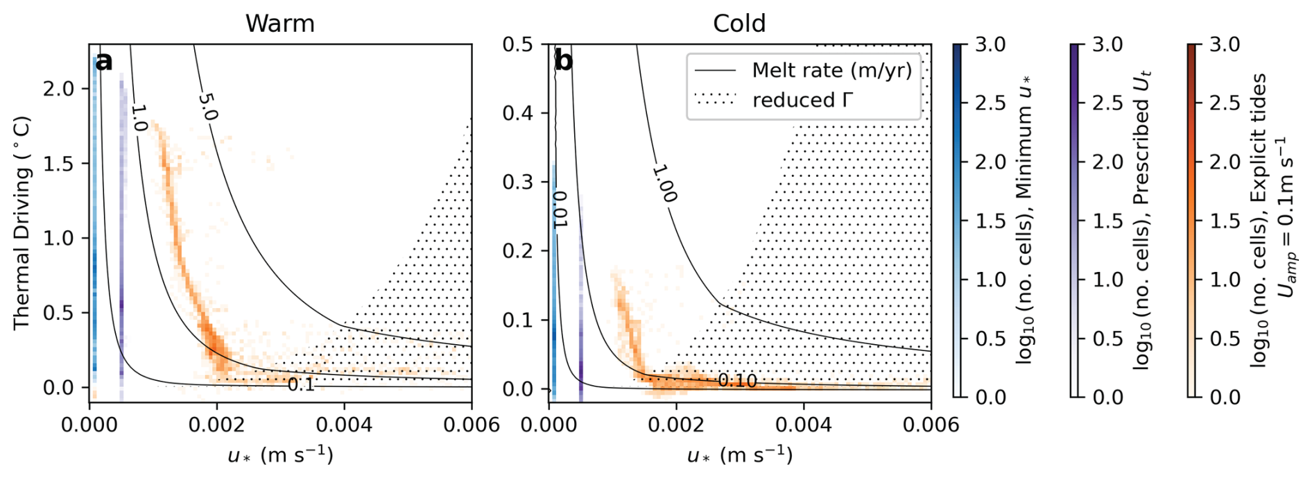
Figure 6 Thermal driving–friction velocity regime diagrams for selected MOM6 StratFeedback experiments, indicating the number of grid cells in each regime time-averaged over the final 180 d of the simulation. Panel (a) shows warm experiments, and panel (b) shows cold experiments. The minimum friction velocity $\mathrm{1}\times {\mathrm{10}}^{-\mathrm{4}}$ m s⁻¹ experiments are shown in blue (leftmost vertical line), prescribed tidal velocity U_t=0.01 m s⁻¹ in purple (middle vertical line) and explicit tidal forcing with amplitude 0.1 m s⁻¹ in orange colours to the right. StratFeedback melt rates are shown by the solid contours, and stippling shows where transfer coefficients are equal to the ConstCoeff values, both calculated assuming a salinity S_M=34.05 psu and pressure 300 dbar, which are representative values for the ISOMIP+ cavity. Note the difference in y-axis extent between panels.

Between MOM6 and MITgcm, the behaviour of the StratFeedback parameterisation under each of the warm, cold and alternative low-velocity limits is consistent, despite melt rates being larger in MITgcm. There are similar percentage decreases in melt rate between the ConstCoeff and StratFeedback experiments despite the variation in the magnitude of melt (Fig. 5). The different magnitude of melt between models may be explained chiefly by the different vertical coordinates (Gwyther et al., 2020), where the z-level coordinates of MITgcm result in a coarser vertical resolution near the ice and therefore a stronger thermal driving since the far-field temperature is sampled at a greater depth but may also be associated with other model choices such as the vertical mixing scheme. Nonetheless, the similar behaviour of the two models demonstrates a consistent response by the new parameterisation on simulated melt rates, circulation and their feedback.

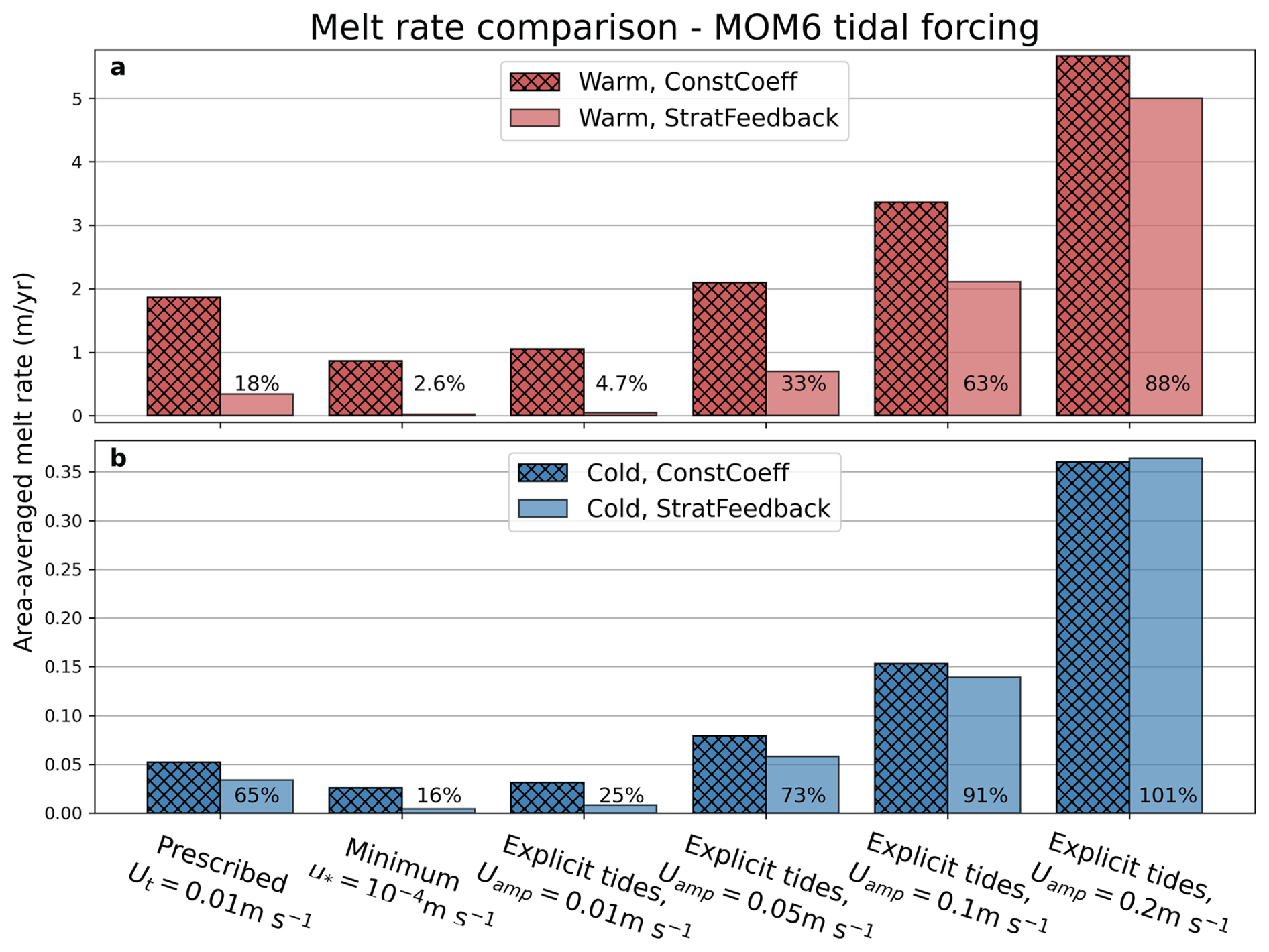
Figure 7 Area-averaged melt rates for MOM6 experiments averaged over the last 180 d of the simulation, with either a prescribed tidal velocity of 0.01 m s⁻¹, a minimum friction velocity of $\mathrm{1}\times {\mathrm{10}}^{-\mathrm{4}}$ m s⁻¹, or both the minimum friction velocity and idealised barotropic tides applied at the open-ocean boundary with velocity amplitudes of 0.01, 0.05, 0.1 and 0.2 m s⁻¹. Warm experiments are shown in panel (a), and cold experiments are shown in panel (b). Hatched bars are experiments with a constant transfer coefficient, and solid colours are with the stratification feedback parameterisation.

4.3 Simulating tides to explore energetic ice shelf cavity regimes

Motivated by the low melt rates in the idealised ISOMIP+ test cases, we replace the prescribed tidal velocities in Fig. 4 with explicit simulation of idealised tides in MOM6. Explicit tides move the experiments to more energetic (and realistic) ice shelf cavity regimes (from the blue and purple to the orange colours in Fig. 6). The cavity circulation is therefore no longer only driven by meltwater buoyancy, and this results in increased melting in both the cold and warm experiments relative to the minimum u_* experiment, which is the control for the tide experiments (Fig. 7, second columns from the left). The magnitude of melting depends on the amplitude of the tidal forcing (Fig. 7). We see that a 0.05 m s⁻¹ amplitude tide gives similar melt rates (within a factor of 1–2) to the prescribed tidal velocity experiment despite the tide amplitude at the boundary being 5 times greater. This occurs because the tidal velocity amplitude adjacent to the ice–ocean interface is smaller than the forced tide at the open boundary (Fig. S1). In this experiment, the root mean square tidal velocity simulated within the cavity is approximately 0.02 m s⁻¹ (see e.g. Anselin et al., 2023, for a derivation of the tidal velocity contribution to u_*), similar to the 0.01 m s⁻¹ prescribed tidal velocity.

The largest warm and cold tidal amplitude ConstCoeff experiments (0.2 m s⁻¹) have at least 3 and 7 times the magnitude of melt, respectively, compared with the warm and cold control cases with prescribed tidal velocity (Fig. 7; compare leftmost and rightmost hatched columns). The proportional increase in melt rate is even greater for the StratFeedback experiments. This can be explained by a shift in the ice shelf cavity regime with the addition of a strong external velocity. Figure 6 shows a shift towards higher friction velocities in the explicit tide experiments (compare the purple and orange colours, the latter of which is the 0.1 m s⁻¹ experiment) and a shift out of the stratified regime and into the well-mixed region of $T^{*}-u^{*}$ parameter space, where the StratFeedback and ConstCoeff parameterisations are equal (indicated by the stippling in Fig. 6, assuming a salinity of S=34.05, and also shown in Fig. 2d). Increased melt in the highest-tide-amplitude experiment also leads to cooling and weaker thermal driving (Fig. 6), further shifting the cavity regime to well-mixed conditions.

The behaviour of the StratFeedback parameterisation as the cavity environment becomes progressively more energetic is shown in Fig. 8. With low or no tidal forcing, much of the cavity sits within the diffusive–convective melt regime (purple colours in Fig. 8). As the tidal amplitude is increased, the stratified (orange colours) and well-mixed (yellow colours) shear-driven melt regimes begin to dominate. For the experiment with the largest tidal forcing, only small regions of the ice shelf cavity are within the stratified or diffusive–convective regimes, and the StratFeedback and ConstCoeff parameterisations give similar melt rates (Fig. 7).

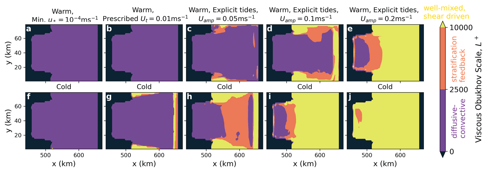
Figure 8 Viscous Obukhov scale, L⁺, regimes for the MOM6 ice shelf region averaged over the last 180 d of the StratFeedback simulations. For each experiment, the diffusive–convective regime is shown in purple and corresponds to $L^{+}<\mathrm{2500}$. The stratification feedback regime is shown in orange, with $\mathrm{2500}<L^{+}<\mathrm{1}\times {\mathrm{10}}^{\mathrm{4}}$, indicating the region where melting is expected to be steady, but the transfer coefficients are suppressed due to the effect of stratification. The well-mixed, shear-driven regime with $L^{+}>\mathrm{1}\times {\mathrm{10}}^{\mathrm{4}}$ and constant (maximal) transfer coefficients is indicated in yellow. Warm experiments are shown in the top row, and cold experiments are shown in the bottom row.

There are additional rectified tidal flows affecting the circulation and hydrography, a discussion of which is beyond the scope of this paper. However, the idealised tidal simulations demonstrate the difficulty in achieving realistic ice shelf cavity regimes in idealised models. Even with a large tidal forcing of 0.2 m s⁻¹ amplitude velocity (corresponding to a 6.4 m sea level anomaly forcing in this idealised cavity), the warm cavity is not entirely in the well-mixed regime, possibly associated with the smoothness of the geometry and insufficient spatial resolution.

4.4 Realistic Pine Island Glacier simulation

To assess the parameterisation in a realistic situation where circulation is more complex, and the results can be compared with observations, we use the MITgcm Pine Island Glacier setup of Nakayama et al. (2021) (model details in Sect. 3.2). We tune the drag coefficient to achieve melt rates similar to the Adusumilli et al. (2020a) satellite melt rate product, though we acknowledge that satellite melt rates contain uncertainties and can differ from in situ ApRES measurements (Vaňková and Nicholls, 2022; Lindbäck et al., 2025). After 20 d of simulation, area-averaged melt rates are approximately equilibrated and of a similar magnitude of ∼17 m yr⁻¹ (as a result of the tuning (Table 2), noting that this rate refers to the whole simulated cavity average rather than the masked area over which melt rates were tuned in Sect. 3.2). We compare the melt rate distributions for three different parameterisation choices averaged over days 20–50. The simulation run with the Holland and Jenkins (1999) parameterisation and McPhee (1981) η_* stability parameter set to 1, hereafter HJ99-neutral, requires the lowest tuned drag coefficient (C_d=0.004), corresponding to the largest average melt rate if tuning is not performed (i.e. using C_d=0.0015 gives an average melt rate of 11.3 m yr⁻¹; Fig. S2a in the Supplement). The StratFeedback parameterisation without tuning yielded a melt rate of 4 m yr⁻¹ (Fig. S2b) and required a larger tuned drag coefficient of C_d=0.0073. This implies that much of the Pine Island Glacier ice shelf is in the stratified regime. Furthermore, when we include the MK18 low-velocity limit in the untuned simulations, the melt rates increase to an average of 8 m yr⁻¹ (Fig. S2c). This melt rate is larger than the untuned StratFeedback simulation because the relatively large ice base slopes (up to 30°) contribute substantial melting via the MK18 parameterisation. Because the untuned StratFeedback simulation has the weakest melting, the tuned StratFeedback simulation has the largest drag coefficient of the three tuned simulations so that the same mean melt rate is achieved. By using the tuned simulations, we can more easily compare spatial distributions of melt rate and the parameterisation's effect on ocean properties. Note the tuned drag coefficients (C_d=0.004 for tuned HJ99-neutral, 0.0073 for tuned StratFeedback and 0.0057 for tuned StratFeedback + MK18) all lie between the value C_d=0.0015 used in the original simulation and the value C_d=0.0097 suggested by Jenkins et al. (2010) (see Sect. 2.1 for more observational estimates of drag coefficients).

In the tuned HJ99-neutral simulation, melt is enhanced near the grounding line (Fig. 9a) and reaches the observed melt rates of up to 200 m yr⁻¹ in this region (Shean et al., 2019; Zinck et al., 2024a, see probability distribution in Fig. D1). Melt is also enhanced at the ice shelf keels (Fig. 9a), as in Shean et al. (2019). Unlike observations which suggest low melt rates in the northern part of the ice shelf, simulated melt rates reach ∼ 50 m yr⁻¹ in this region (compare Figs. 9a and D1b, c). The difference suggests there may be differences between the simulated and real pathways of water masses into the northern section of the Pine Island Glacier ice shelf cavity.

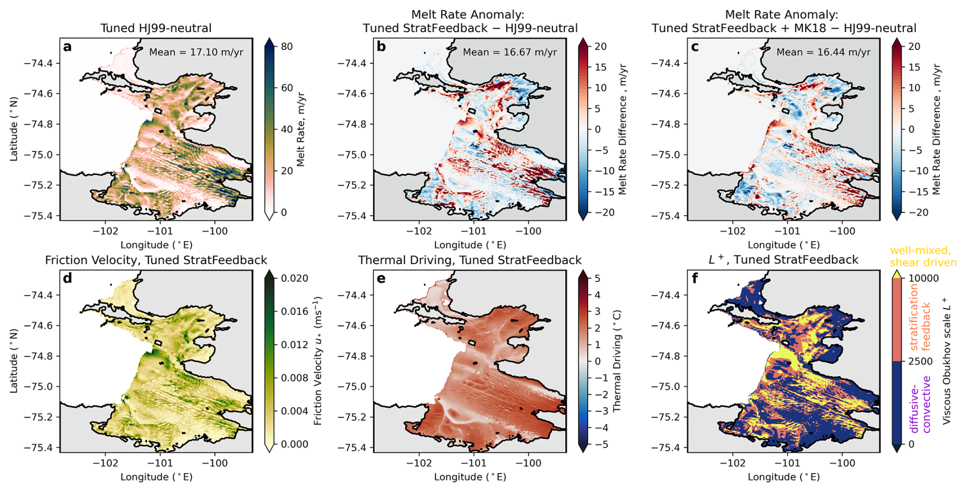
Figure 9 MITgcm Pine Island Glacier melt rates averaged over days 20–50 of the simulation for (a) the tuned HJ99-neutral basal melt parameterisation used in Nakayama et al. (2021) (with a drag coefficient of C_d=0.004), (b) the anomaly of the tuned stratification feedback (StratFeedback) parameterisation (with a drag coefficient of C_d=0.0073) and (c) the anomaly of the tuned stratification feedback parameterisation with MK18 limit (with a drag coefficient of C_d=0.0057). Both anomalies in (b) and (c) are with respect to (a). The melt rates quoted are calculated over the whole simulated ice shelf area and differ from the tuning melt rate, which was only over the region where Adusumilli et al. (2020a) data are present (Fig. D1b) and only south of 74.8°S. The friction velocity, thermal driving and viscous Obukhov scales of the stratification feedback parameterisation with tuned drag coefficient (b) are shown in panels (d), (e) and (f).

In the tuned StratFeedback simulation, the melt rates are increased relative to the tuned HJ99-neutral simulation in some regions, such as near the Pine Island Glacier grounding line and in the ice shelf keels (and some channels with high velocities), and decreased elsewhere (Fig. 9b). The regions where the tuned StratFeedback simulation enhances melt correspond to regions with large friction velocities (Fig. 9d), and melt decreases in regions with low friction velocities, including some regions near the grounding line. In the large-friction-velocity regions, L⁺ is also large (Fig. 9f), indicating melting in the well-mixed regime, whereas regions with lower friction velocities have lower L⁺ and are simulated to be in the stratified and diffusive–convective regimes. The StratFeedback parameterisation therefore enhances the spatial variability in melt beneath Pine Island Glacier. Ocean properties and circulation respond to this modified melt rate, leading to fresher, colder water in regions with more melting (see Supplement Figs. S3, S4, S5).

The tuned StratFeedback + MK18 simulation has a similar melt rate anomaly pattern to the tuned StratFeedback simulation. However, in addition to having enhanced melt in regions with large friction velocity compared to the HJ99-neutral experiment, melt is also enhanced at the sloped ice shelf front and near the grounding line, the latter where the thermal driving is large (Fig. 9e). Both the tuned StratFeedback and StratFeedback + MK18 experiments have a larger area of the ice shelf with melting greater than 50 m yr⁻¹ compared with the tuned HJ99-neutral simulation (Fig. D1) and align better with the melt rates on the order of 100 m yr⁻¹ seen in high-resolution observational products near the grounding line (Zinck et al., 2024a; Shean et al., 2019). This improvement is demonstrated by the upper tail of the melt rate statistical distribution (Fig. D1) increasing in area with the StratFeedback parameterisation, bringing the distribution closer to the Zinck et al. (2024a) product. The missing data and coarser resolution of Adusumilli et al. (2020a) make quantitative comparison challenging. The general similarity between StratFeedback and StratFeedback + MK18 also indicates that large parts of the tuned Pine Island Glacier simulations are not in the low-velocity regime (with the diffusive–convective regime as a guide in Fig. 9f).

The difference in the spatial distribution of melt rates between the original simulation and that with the StratFeedback parameterisation highlights the spatial heterogeneity in melt rate regimes within individual ice shelves. All three regimes – well-mixed–shear-driven, stratified and diffusive–convective – were observed in the tuned simulations (Fig. 9f). Analysis of borehole observations from Pine Island Glacier yielded a shear-driven L⁺ of 1.1×10⁴ (Fig. 3b), which was taken in one of the channels approximately halfway between the ice front and grounding zone (Stanton et al., 2013). Without the precise location on the ice shelf (and noting differences in the time of simulation and observation), it is difficult to determine if the simulated channels' L⁺ agree with the observation. However, keels and some channels are generally simulated to be in the shear-driven regime, potentially in agreement with Stanton et al. (2013). Nevertheless, the need for significantly different drag coefficients between tuned simulations demonstrates the sensitivity of regional ice shelf models' basal melting and melt regimes to parameterisations.

5 Discussion

In this study, we describe the development and implementation of a basal melt parameterisation that includes the feedback effect of stratification suppressing turbulence at the ice–ocean boundary layer in ocean models. Our transfer coefficients use empirical functional forms based on large eddy simulations (Vreugdenhil and Taylor, 2019; Rosevear et al., 2022b, Fig. 1). Compared with a constant transfer coefficient formulation, predicted melt rates are suppressed under low-velocity and warm-ice-shelf-cavity conditions (Fig. 2), where stratification feedback effects on melt are expected to be stronger, due to the relatively higher melt (strengthening the stratification). This results in improved melt rates compared to observations for ice shelf cavities in the stratified but still shear-driven or diffusive–convective ice shelf cavity regimes, particularly the Amery Ice Shelf (Fig. 3). The parameterisation therefore decreases the disagreement between direct melt rate observations and parameterisations in some ice shelf cavity regimes and leaves them unchanged in others.

We tested the stratification feedback melt parameterisation in model configurations of varying complexity and ice shelf cavity regimes. Compared with the constant-coefficient formulation, idealised ISOMIP+ experiments in MOM6 and MITgcm saw significant reductions in melt and circulation strength in both the warm and cold simulations (Fig. 5). The melt rate reduction demonstrated that the ISOMIP+ experiments are simulated to be in a quiescent, warm regime with a low viscous Obukhov scale (Figs. 6, 8), with the stratification feedback parameterisation suppressing melt as a result. This can be explained by the buoyancy-only ISOMIP+ setup, where there are no external forcings (except for a restoring sponge layer), and therefore the circulation is driven only by the buoyant meltwater plume. When an idealised external forcing was applied, with a barotropic tidal forcing in MOM6, melt rates increased as in Gwyther et al. (2016), and regions of the ice shelf cavity moved into the more energetic, shear-driven regime (Figs. 6, 7, 8) where the stratification feedback was less pronounced. However, even with explicit tides, our ISOMIP+ experiments could not achieve the thermal driving and friction velocity conditions observed at George VI and Pine Island Glacier ice shelves, nor could the summer Ross Ice Shelf observations of Stewart (2018) (compare Figs. 3 and 6). This result suggests that idealised ocean models should be used with caution when assessing melt parameterisations or other ice shelf boundary layer physics or indeed other aspects of ice shelf cavity circulation.

The melt rate (and therefore ocean circulation) is sensitive to melt parameterisation choices at the low-velocity limit, primarily because of the low velocities (and L⁺) in the smooth, idealised ISOMIP+ cavity. The StratFeedback parameterisation, though designed for the stratified regime, suppresses melt rates in the diffusive–convective regime and better matches observations and simulations in this regime (Fig. 3; Begeman et al., 2018) but is still an extrapolation in these low-velocity conditions. Attempts to connect the shear-driven melt parameterisation (with StratFeedback or ConstCoeff transfer coefficients) and previously suggested free-stream velocity-independent convective melt scaling (Kerr and McConnochie, 2015; McConnochie and Kerr, 2018; Mondal et al., 2019; Schulz et al., 2022) led to higher melt rates (Fig. 5) than with the chosen minimum friction velocity, but the idealised model framework made assessing the accuracy of the parameterisation in the context of realistic observations and models difficult. The optimum low-velocity limit for melt parameterisations is still unknown, and awareness of this sensitivity to parameterisation choices is important when simulating cavities with low velocities.

A realistic simulation of Pine Island Glacier compared the stratification feedback parameterisation and HJ99-neutral parameterisation, with both tuned to area-averaged satellite-derived melt rates (Fig. 9), requiring large modifications to the drag coefficient, a significant unconstrained parameter. The StratFeedback and StratFeedback + MK18 parameterisations had stronger peaks of melt rates in the Pine Island keels and near the grounding line, moving the simulated melt rate pattern closer to observations (Shean et al., 2019; Adusumilli et al., 2020a; Zinck et al., 2024a), though a lack of satellite melt rate estimates near the grounding line makes quantitative comparison difficult. The MK18 version has more consistent melt rate intensification near the grounding line than StratFeedback alone, but further work is required to evaluate these parameterisations in other ice shelf cavities and with more observations.

Our results demonstrate the importance of testing basal melt parameterisations across various ice shelf cavity regimes. The basal melt–ocean circulation positive feedback makes idealised models extremely sensitive to specific choices in the parameterisation, possibly more so than realistic models. Still, achieving the expected L⁺ suggested by in situ borehole observations, where many locations had conditions with $L^{+}>{\mathrm{10}}^{\mathrm{4}}$ (Fig. 3b), required large drag coefficients in the Pine Island Glacier experiment, despite the relatively high model resolution. Ocean models, particularly coarse-resolution models, may lack the small-scale flow variability observed at high frequencies beneath ice shelves, either through not resolving these scales of motion (through both horizontal and vertical resolution), not simulating tidal motion, or having anomalously smooth bathymetry and ice base shape. Our results suggest that one reason current parameterisations in ocean models do achieve relatively good agreement with satellite-derived melt rates (Richter et al., 2022; Galton-Fenzi et al., 2025) might be a compensation of biases: if simulated velocities are weaker than reality and constant transfer coefficients larger than reality, the ConstCoeff basal melt transfer velocities might be of the correct magnitude. This compensation, however, would be expected to depend on resolution; future research should investigate the model grid resolution dependence of simulated ice shelf regimes. Understanding this dependence is particularly important for the MK18 parameterisation, which is based on local slope and is therefore resolution-dependent. Unravelling this compensation led to low melt rates in our StratFeedback parameterisation before drag coefficient tuning, highlighting the need for more high-resolution ice shelf cavity simulations.

Furthermore, the difference between MOM6 and MITgcm ISOMIP+ experiments demonstrates the ongoing challenge in unifying parameterisations when ocean models simulate the ice shelf ocean boundary layer differently. Specifically, the vertical resolution and coordinate are important factors, where appropriate choices (using high vertical resolution and appropriately sampling the far-field ocean properties and distributing meltwater) can reduce the sensitivity of simulated melt to model choices (Gwyther et al., 2020; Scott et al., 2023).

There remain questions around formulating a regime-aware, physically accurate basal melt parameterisation. Future work should further explore the transition between the shear-controlled stratified regime and the transient diffusive–convective regime (e.g. Rosevear et al., 2022b). We have proposed one option for a transition to a velocity-independent convective parameterisation at low velocities, where the McConnochie and Kerr (2018) parameterisation increases melt rates near sloped ice bases (and therefore better matches satellite-derived melt rates at the Pine Island Glacier grounding line). However, this parameterisation's applicability to weakly sloped ice bases remains unknown, and the representation of sloping or featured topography depends on the resolution of ice draft products and the resolution at which the model is run. Prescribed tidal velocities and minimum friction velocities are also easily implemented low-velocity limit options, which could be tuned in realistic experiments. However, both melting and circulation are likely to be sensitive to these unconstrained parameters. Furthermore, other physical processes such as diffusive convection are currently not included. Developing a truly regime-aware parameterisation likely requires further understanding of the physics governing each regime and the transitions, through more high-resolution numerical simulations, laboratory experiments and in situ ice shelf–ocean boundary layer observations. For example, conducting similar experiments to Rosevear et al. (2022b) that resolve the boundary layer with shallow ice slopes would fill a currently undersampled regime. Davis et al. (2025) also recently demonstrated the importance of lateral processes within the ice–ocean boundary layer of warm-cavity ice shelves, which ice shelf basal melt parameterisations do not include.

The Pine Island Glacier simulation experiments highlight an outstanding unknown in basal melt parameterisations: the drag coefficient. Further work is required to understand the spatial distribution of drag coefficients around Antarctic ice shelves and how we can model the momentum boundary layer and its effect on melting in ocean models with varying vertical resolution and coordinates rather than treating it as a tuning coefficient. Additionally, the transfer and drag coefficients for refreezing (Galton-Fenzi et al., 2012; Gwyther et al., 2016; McPhee et al., 2016) and the effect of heat conduction into the ice shelf (Holland and Jenkins, 1999; Wiskandt and Jourdain, 2025) are also important data-poor factors we have not explored.

This work has focused on basal melt parameterisations in ocean models, but there is also scope to translate the effect of stratified melt rate feedbacks into basal melt parameterisations for stand-alone ice sheet models, where ice shelf basal melt parameterisations tend to be even further simplified than in ocean models (e.g. Burgard et al., 2022). Improving the accuracy of our climate and earth system models will require ongoing development of regime-aware basal melt parameterisations and implementation in large-scale models.

6 Conclusions

We implemented a basal melt parameterisation which accounts for turbulence suppression due to stratification in the ice shelf-ocean boundary layer in two ocean models. Our main findings discussed in this article are that

• the stratification feedback suppresses melt rates in the idealised ISOMIP+ model experiments compared with the control, constant-coefficient melt parameterisation;

• the change in melt rate between the constant-coefficient and stratification feedback parameterisations depends on the cavity conditions, including the temperature and presence of external tidal forcing, as well as the choice of low-velocity limit in the melt parameterisation, and is sensitive to the strong feedback with ice shelf cavity circulation;

• when tested in a Pine Island Glacier simulation, the spatial distribution of melt was modified by the stratification feedback parameterisation, and the melt rate was decreased to 40 % of the original parameterisation without further tuning of the drag coefficient; with drag coefficient tuning, the melt rate becomes intensified at glacial keels and near the grounding line, with higher peak melt rates moving closer to satellite observational estimates.

Accurate simulation of Antarctic ice shelf basal melting will require further work to optimise basal melt parameterisations across ice shelf cavities in different thermal and energetic conditions. This will be particularly important in warm cavities with weak flows, where there are large uncertainties in the transitions between ice shelf cavity regimes. Future work should also aim to identify biases in ice shelf cavity regimes in realistic ocean model simulations and explore how the effect of these biases on melt rate may be addressed.

Appendix A: Melt rate parameterisation design

Here, we provide further details on the melt parameterisation formulations. Table A1 presents relevant constants, variables and parameters in addition to Table 1.

McConnochie and Kerr (2018)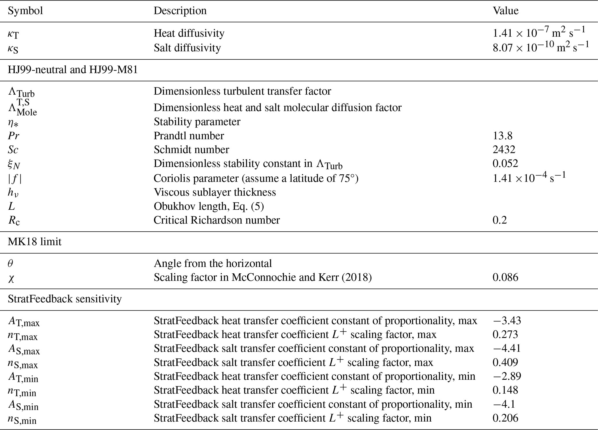

Table A1 Table of constants, variables and parameters for Appendix A, in addition to Table 1.

A1 Holland and Jenkins (1999) parameterisation and McPhee (1981) stability parameter

We review the Holland and Jenkins (1999) (HJ99) parameterisation and McPhee (1981) stability parameter, referred to in this study as HJ99-M81. These studies use both thermodynamics and Monin–Obukhov boundary layer scalings (Monin and Obukhov, 1954) to quantify momentum as well as salt and heat transport over the boundary layer. Building on Kader and Yaglom (1972), McPhee et al. (1987), and others, HJ99 express the transfer velocities used in the three-equation parameterisation (Eqs. 1–3) as

$$\begin{array}{}\text{(A1)}& {\mathit{\gamma }}_{T,S}={\displaystyle \frac{u_{*}}{{\mathrm{\Lambda }}_{\text{Turb}}+{\mathrm{\Lambda }}_{\text{Mole}}^{T,S}}},\end{array}$$

where we use Λ to denote the dimensionless factors rather than the original HJ99 Γ notation to avoid confusion with Eq. (4). Here, ${\mathrm{\Lambda }}_{\text{Mole}}^{T,S}$ represents heat and salt transfer associated with molecular diffusion,

$$\begin{array}{}\text{(A2)}& {\displaystyle }{\mathrm{\Lambda }}_{\text{Mole}}^T=\mathrm{12.5}(\mathit{Pr}{)}^{\mathrm{2}/\mathrm{3}}-\mathrm{6},\text{(A3)}& {\displaystyle }{\mathrm{\Lambda }}_{\text{Mole}}^S=\mathrm{12.5}(\mathit{Sc}{)}^{\mathrm{2}/\mathrm{3}}-\mathrm{6},\end{array}$$

with Pr the Prandtl number $\mathit{\nu }/{\mathit{\kappa }}_{\mathrm{T}}$ and Sc the Schmidt number $\mathit{\nu }/{\mathit{\kappa }}_{\mathrm{S}}$ (refer to Table A1 for constants and values). Λ_Turb represents transfer associated with turbulence,

$$\begin{array}{}\text{(A4)}& {\mathrm{\Lambda }}_{\text{Turb}}={\displaystyle \frac{\mathrm{1}}{k}}\ln \left({\displaystyle \frac{u_{*}{\mathit{\xi }}_N{\mathit{\eta }}_{*}^{\mathrm{2}}}{f{h}_{\mathit{\nu }}}}\right)+{\displaystyle \frac{\mathrm{1}}{\mathrm{2}{\mathit{\xi }}_N{\mathit{\eta }}_{*}}}-{\displaystyle \frac{\mathrm{1}}{k}}.\end{array}$$

Here, ξ_N is a dimensionless constant; h_ν is the viscous sublayer thickness, estimated as $h_{\mathit{\nu }}=\mathrm{5}\mathit{\nu }/u_{*}$; and η_* is the McPhee (1981) stability parameter designed to account for stabilising buoyancy fluxes

$$\begin{array}{}\text{(A5)}& {\mathit{\eta }}_{*}={\left(\mathrm{1}+{\displaystyle \frac{{\mathit{\xi }}_N{u}_{*}}{\left|f\right|L{R}_c}}\right)}^{-\mathrm{1}/\mathrm{2}}.\end{array}$$

Refer to Table A1 for definitions. The melt parameterisation contains constant parameters, η_* (a function of friction velocity and buoyancy) and the friction velocity, so it is a variable transfer coefficient. In most ocean models that use the HJ99 parameterisation (Losch, 2008; Dansereau et al., 2014), η_* is set to 1, representing neutral conditions (which we refer to as HJ99-neutral parameterisation). HJ99-neutral has varying transfer coefficients due to the dependence on friction velocity, but with much less variability than the StratFeedback parameterisation (within 10 % of ConstCoeff melt rates under most relevant conditions). Figure A1a shows this reduced variability by plotting the ratio of melt rate calculated with HJ99-neutral under different thermal driving and friction velocity conditions with that from the ConstCoeff parameterisation, as a comparison with Fig. 2d. If we allow η_* to vary (the HJ99-M81 form) and compare melt rates with those from the ConstCoeff parameterisation (Fig. A1c), we can see that melting is suppressed under very low-friction-velocity and high-thermal-driving conditions (also shown in Fig. A1b, comparing with HJ99-neutral). However, this suppression is less extreme and far less extensive in regime space than the empirically derived StratFeedback parameterisation (Fig. 2d).

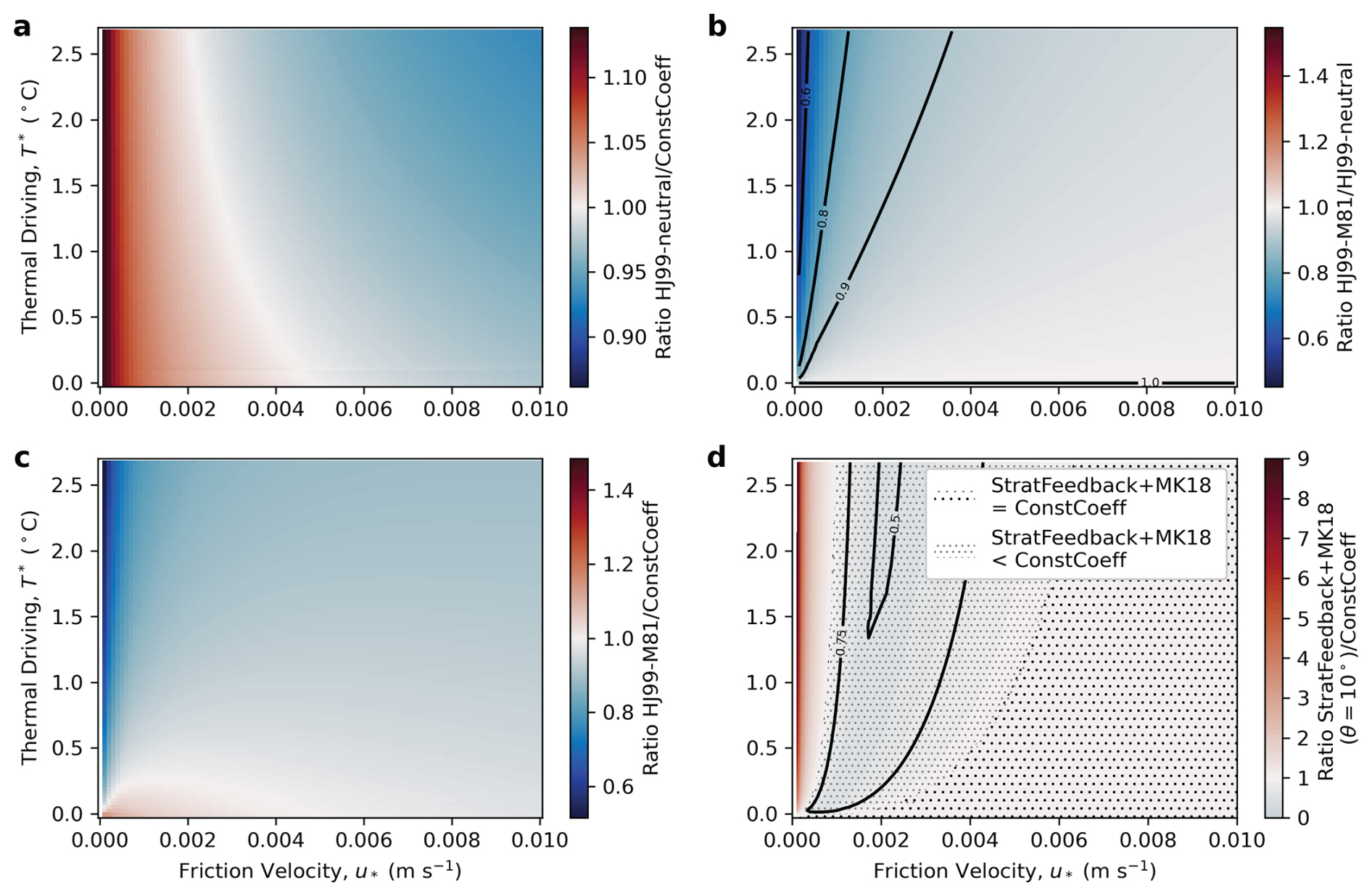
Figure A1 Ratio of melt rate calculated from varying transfer coefficient methods to the constant-coefficient parameterisation used in this study, presented in thermal driving–friction velocity regime space, assuming S_M=34.5 and a pressure of 500 dbar (∼ 500 m depth). Panel (a) shows the Holland and Jenkins (1999) parameterisation with the McPhee (1981) stability parameter (Appendix A1) set to 1 (neutral conditions), and panel (c) shows it with the McPhee (1981) stability parameter varying. The difference between HJ99-M81 and HJ99-neutral is shown in panel (c). Panel (d) shows the combined stratification feedback and McConnochie and Kerr (2018) low-velocity limit with $\mathit{\theta }={\mathrm{10}}^{\circ }$ (Sect. 2.5, Appendix A3) compared to ConstCoeff. Contours at ratios 0.5 and 0.75 are provided.

A2 StratFeedback parameterisation sensitivity

There is considerable uncertainty in fitting to the LES results of Fig. 1. To test the sensitivity of the choice of parameterisation fit to the modelled melt rates, we ran sensitivity experiments with a steeper (max) and shallower (min) line of best fit, where the max and min versions were obtained by changing the critical L⁺ from 1×10⁴ to 5×10³ and 5×10⁴, respectively. The corresponding fit parameters for the StratFeedback transfer coefficients are presented in Table A1. The results of this uncertainty in melt rate for the ISOMIP+ style experiments with a prescribed tidal velocity in MOM6 are presented as uncertainty bars in Fig. 5, indicating that the qualitative results are not sensitive to the exact values of the empirical fit of LES results.

A3 Transition to McConnochie and Kerr (2018) parameterisation

To transition smoothly between the shear-driven three-equation parameterisation and a velocity-independent melt parameterisation of McConnochie and Kerr (2018) (MK18) and Mondal et al. (2019), we reformulate the MK18 melt rate in terms of an effective transfer velocity that depends on temperature, salinity, ice base slope and constants.

Using laboratory experiments and theoretical models, MK18 and Kerr and McConnochie (2015) estimate the difference in temperature of the far-field T_M and interface T_b to be

$$\begin{array}{}\text{(A6)}& T_{\mathrm{M}}-T_{\mathrm{b}}={\displaystyle \frac{{\mathit{\rho }}_{\mathrm{I}}L+{\mathit{\rho }}_{\mathrm{I}}{c}_{p,\mathrm{I}}(T_{\mathrm{b}}-T_{\mathrm{I}})}{{\mathit{\rho }}_{\mathrm{M}}{c}_{p,\mathrm{M}}}}{\left({\displaystyle \frac{{\mathit{\kappa }}_{\mathrm{s}}}{{\mathit{\kappa }}_{\mathrm{T}}}}\right)}^{\mathrm{1}/\mathrm{2}}\left({\displaystyle \frac{S_{\mathrm{M}}-S_{\mathrm{b}}}{S_{\mathrm{M}}-S_{\mathrm{I}}}}\right),\end{array}$$

where we modify the notation to match Sect. 2.1, so subscripts b, M and I are the boundary, far-field and ice. κ_s is the compositional diffusivity (salt), whilst κ_T is the heat diffusivity.

The ice ablation velocity, or melt rate, is

$$\begin{array}{}\text{(A7)}& m=\mathit{\chi }{\sin }^{\mathrm{2}/\mathrm{3}}\mathit{\theta }{\left({\displaystyle \frac{g({\mathit{\rho }}_{\mathrm{M}}-{\mathit{\rho }}_{\mathrm{b}}){\mathit{\kappa }}_{\mathrm{s}}^{\mathrm{2}}}{\mathit{\mu }}}\right)}^{\mathrm{1}/\mathrm{3}}\left({\displaystyle \frac{S_{\mathrm{M}}-S_{\mathrm{b}}}{S_{\mathrm{M}}-S_{\mathrm{I}}}}\right),\end{array}$$

where χ is a non-dimensional constant from the laboratory experiments of McConnochie and Kerr (2018), θ is the angle of the base measured from the horizontal and μ=νρ₀ the dynamic viscosity (Table A1). Note that McConnochie and Kerr (2018) do not test shallow slope angles and that with very low slope angles the ice ablation is more likely to be dominated by current shear than buoyant convection since buoyancy forces decrease as slope angles become lower (Rosevear et al., 2025). However, Mondal et al. (2019) also suggest a ${\sin }^{\mathrm{2}/\mathrm{3}}\mathit{\theta }$ scaling for turbulent boundary layer flows (and a ${\sin }^{\mathrm{1}/\mathrm{4}}\mathit{\theta }$ scaling for laminar flows) for a wider range of slope angles (2–90° from the horizontal).

We can approximate the density change in Eq. (A7) with a linear equation of state:

$$\begin{array}{}\text{(A8)}& {\mathit{\rho }}_{\mathrm{M}}-{\mathit{\rho }}_{\mathrm{b}}\approx \mathit{\beta }{\mathit{\rho }}_{\mathrm{0}}\left(S_{\mathrm{M}}-S_{\mathrm{b}}\right)-\mathit{\alpha }{\mathit{\rho }}_{\mathrm{0}}\left(T_{\mathrm{M}}-T_{\mathrm{b}}\right).\end{array}$$

Equation (A7) can then be rearranged as

$$\begin{array}{}\text{(A9)}& \begin{array}{rl}{\mathit{\rho }}_{\mathrm{I}}{S}_{\mathrm{b}}m& =\mathit{\chi }{\sin }^{\mathrm{2}/\mathrm{3}}\mathit{\theta }{\left({\displaystyle \frac{\begin{array}{c}g{\mathit{\rho }}_{\mathrm{0}}(\mathit{\beta }\left(S_{\mathrm{M}}-S_{\mathrm{b}}\right)-\\ \mathit{\alpha }\left(T_{\mathrm{M}}-T_{\mathrm{b}}\right)){\mathit{\kappa }}_{\mathrm{s}}^{\mathrm{2}}\end{array}}{\mathit{\nu }{\mathit{\rho }}_{\mathrm{0}}}}\right)}^{\mathrm{1}/\mathrm{3}}\left({\displaystyle \frac{S_{\mathrm{M}}-S_{\mathrm{b}}}{S_{\mathrm{M}}-S_{\mathrm{I}}}}\right){\mathit{\rho }}_{\mathrm{I}}{S}_{\mathrm{b}}\\ & =\underset{{\mathit{\gamma }}_{\mathrm{S}},\text{eff}}{\underbrace{\mathit{\chi }{\sin }^{\mathrm{2}/\mathrm{3}}\mathit{\theta }{\left({\displaystyle \frac{\begin{array}{c}g(\mathit{\beta }\left(S_{\mathrm{M}}-S_{\mathrm{b}}\right)-\\ \mathit{\alpha }\left(T_{\mathrm{M}}-T_{\mathrm{b}}\right)){\mathit{\kappa }}_{\mathrm{s}}^{\mathrm{2}}\end{array}}{\mathit{\nu }}}\right)}^{\mathrm{1}/\mathrm{3}}\left({\displaystyle \frac{{\mathit{\rho }}_{\mathrm{I}}{S}_{\mathrm{b}}}{{\mathit{\rho }}_{\mathrm{0}}\left(S_{\mathrm{M}}-S_{\mathrm{I}}\right)}}\right)}}{\mathit{\rho }}_{\mathrm{0}}\left(S_{\mathrm{M}}-S_{\mathrm{b}}\right).\end{array}\end{array}$$

We also neglect the heat capacity term with the ice conduction, as we have done with the shear-driven parameterisation (Sect. 2.3), as it is unlikely to qualitatively change the results when comparing melt parameterisations. Combining Eqs. (A6) and (A7), we can rewrite the melt rate as a function of the temperature difference term:

$$\begin{array}{}\text{(A10)}& \begin{array}{rl}m& =\mathit{\chi }{\sin }^{\mathrm{2}/\mathrm{3}}\mathit{\theta }{\left({\displaystyle \frac{g\left({\mathit{\rho }}_{\mathrm{M}}-{\mathit{\rho }}_{\mathrm{b}}\right){\mathit{\kappa }}_{\mathrm{s}}^{\mathrm{2}}}{\mathit{\nu }{\mathit{\rho }}_{\mathrm{0}}}}\right)}^{\mathrm{1}/\mathrm{3}}\left(T_{\mathrm{M}}-T_{\mathrm{b}}\right)\\ & {\displaystyle \frac{\mathrm{1}}{\frac{{\mathit{\rho }}_{\mathrm{I}}L+{\mathit{\rho }}_{\mathrm{I}}{c}_{p,\mathrm{I}}\left(T_{\mathrm{b}}-T_{\mathrm{I}}\right)}{{\mathit{\rho }}_{\mathrm{M}}{c}_{p,\mathrm{M}}}{\left(\frac{{\mathit{\kappa }}_{\mathrm{s}}}{{\mathit{\kappa }}_{\mathrm{T}}}\right)}^{\mathrm{1}/\mathrm{2}}}}\\ & ={\displaystyle \frac{c_{p,\mathrm{M}}{\mathit{\rho }}_{\mathrm{M}}}{L{\mathit{\rho }}_{\mathrm{I}}}}\left(T_{\mathrm{M}}-T_{\mathrm{b}}\right)\\ & \underset{{\mathit{\gamma }}_{\text{T,eff}}}{\underbrace{\mathit{\chi }{\sin }^{\mathrm{2}/\mathrm{3}}\mathit{\theta }{\left({\displaystyle \frac{g\left(\mathit{\beta }\left(S_{\mathrm{M}}-S_{\mathrm{b}}\right)-\mathit{\alpha }\left(T_{\mathrm{M}}-T_{\mathrm{b}}\right)\right)}{\mathit{\nu }}}\right)}^{\mathrm{1}/\mathrm{3}}{\mathit{\kappa }}_{\mathrm{s}}^{\mathrm{1}/\mathrm{6}}{\mathit{\kappa }}_{\mathrm{T}}^{\mathrm{1}/\mathrm{2}}}}.\end{array}\end{array}$$

In this way, we define effective transfer velocities corresponding to the convective flow limit that may be more appropriate than the shear-driven melt transfer velocities ${\mathit{\gamma }}_{\mathrm{T},\mathrm{S}}=u_{*}{\mathrm{\Gamma }}_{\mathrm{T},\mathrm{S}}$ at low velocities.

The ratio of ${\mathit{\gamma }}_{\mathrm{T}}/{\mathit{\gamma }}_{\mathrm{S}}$ is then

$$\begin{array}{}\text{(A11)}& {\displaystyle \frac{{\mathit{\gamma }}_{\mathrm{T}}}{{\mathit{\gamma }}_{\mathrm{S}}}}={\displaystyle \frac{{\mathit{\rho }}_{\mathrm{0}}{\mathit{\kappa }}_{\mathrm{s}}^{\mathrm{1}/\mathrm{6}}{\mathit{\kappa }}_{\mathrm{T}}^{\mathrm{1}/\mathrm{2}}(S_{\mathrm{M}}-S_{\mathrm{I}})}{{\mathit{\kappa }}_{\mathrm{s}}^{\mathrm{2}/\mathrm{3}}{\mathit{\rho }}_{\mathrm{I}}{S}_{\mathrm{b}}}}={\displaystyle \frac{{\mathit{\rho }}_{\mathrm{0}}{S}_{\mathrm{M}}}{{\mathit{\rho }}_{\mathrm{I}}{S}_{\mathrm{b}}}}\sqrt{{\displaystyle \frac{{\mathit{\kappa }}_{\mathrm{T}}}{{\mathit{\kappa }}_{\mathrm{S}}}}},\end{array}$$

which for values given in Tables 1 and A1 gives ∼ 20, smaller than the ratio in the well-mixed regime of ∼ 30 but in agreement with the StratFeedback parameterisation in the diffusive–convective regime (Fig. 1c).

To connect this velocity-independent parameterisation with the shear-driven formulation, we choose to take the greater of the MK18 effective transfer velocities and the shear-driven $u_{*}{\mathrm{\Gamma }}_{\mathrm{T},\mathrm{S}}$, where the MK18 formulation will be the larger of the two at small friction velocities. Since the MK18 effective transfer velocity depends on the boundary salinity and temperature, iteration will be required to converge to a solution for melt rate. This regime-aware parameterisation is shown in Fig. 2d, where the melt rate contours follow the shear-driven formulations (either StratFeedback or ConstCoeff) at higher friction velocities before transitioning to the velocity-independent melt rate under low-velocity conditions. This parameterisation depends on slope angle, and the local slope angle can be calculated from the ice base taking the maximal local angle.

The effect of the MK18 limit combined with the StratFeedback parameterisation on melt rate is compared with the ConstCoeff parameterisation in Fig. A1d. As in Fig. 2c, melt rates are identical to ConstCoeff under cold and fast conditions (large stippling). Moving to slower conditions in the stratified regime, melt rates are suppressed according to the StratFeedback parameterisation (small stippling). However, under very low-velocity conditions, melt rates are enhanced compared with the ConstCoeff parameterisation due to the MK18 limit (red colours). Note this does not mean melt rates increase with decreasing velocity; rather they become independent of velocity (Fig. 2b), whereas the ConstCoeff melt rate continues to decrease.

Figure A2 presents alternative angle options to the 10° slope used in Figs. 2b and A1d.

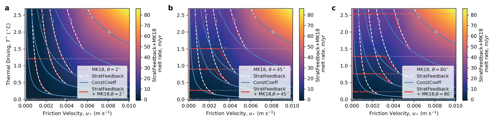
Figure A2 Thermal driving–friction velocity parameter space diagram indicating melt rates calculated as a function of far-field temperature, salinity and pressure (which are set to S=34.5 psu and p=500 dbar) and friction velocity. The melt rates are solved for a variety of parameterisation options: ConstCoeff is shown by the solid blue lines, and StratFeedback is shown by the dashed white lines. Constant melt rates obtained from slope-dependent McConnochie and Kerr (2018) convective parameterisation are shown by the dotted pink lines, and the combination of the StratFeedback + MK18 limit is shown by the dash-dot red line. The three panels show different slope angle choices to Fig. 2b, with angles from the horizontal of (a) 2°, (b) 45° and (c) 80°.

Appendix B: Observational data

Table B1 presents the observational data and computed melt rates used in Fig. 3. Note that parameterised melt rates (ConstCoeff and StratFeedback) and thermal driving may differ from calculated melt rates in the original references due to different choices of drag and transfer coefficients, as well as uncertainty in hydrographic properties, instruments and collection of the data from the references (labelled by ^a). We do not perform an uncertainty analysis, but there is considerable uncertainty in the computed melt rates and observed melt rates, and observations are localised and may not represent conditions throughout each ice shelf.

Where data were not reported as conservative temperature or absolute salinity, we have converted the values using the Gibbs Seawater Oceanographic Toolbox (McDougall and Barker, 2011). This choice was made for consistency to match the most recent studies presented (Begeman et al., 2018; Rosevear et al., 2022a; Davis et al., 2023), noting the variety and evolution in thermodynamic variables used previously. However, the choice does not significantly impact results. The thermodynamic variables used in the observational comparison differ from those used in the models, potential temperature and practical salinity, but we use the same linear freezing point equation of state coefficients throughout the study (Table 1).

Rosevear et al. (2022a)Jenkins et al. (2010)Davis and Nicholls (2019)Stewart (2018)Stewart (2018)Begeman et al. (2018)Kimura et al. (2015)Davis et al. (2023)Stanton et al. (2013)

Table B1 Table of input and computed values for borehole observation and melt rate parameterisation comparison in Fig. 3. Conservative temperature T_M, pressure p, absolute salinity S_M and far-field velocity U_M were obtained from the references as time-mean ice shelf far-field input variables for the three-equation parameterisation, and the computed thermal driving T^* and melting under the ConstCoeff (CC) and StratFeedback (SF) parameterisations are presented, as are the directly observed melt rates.

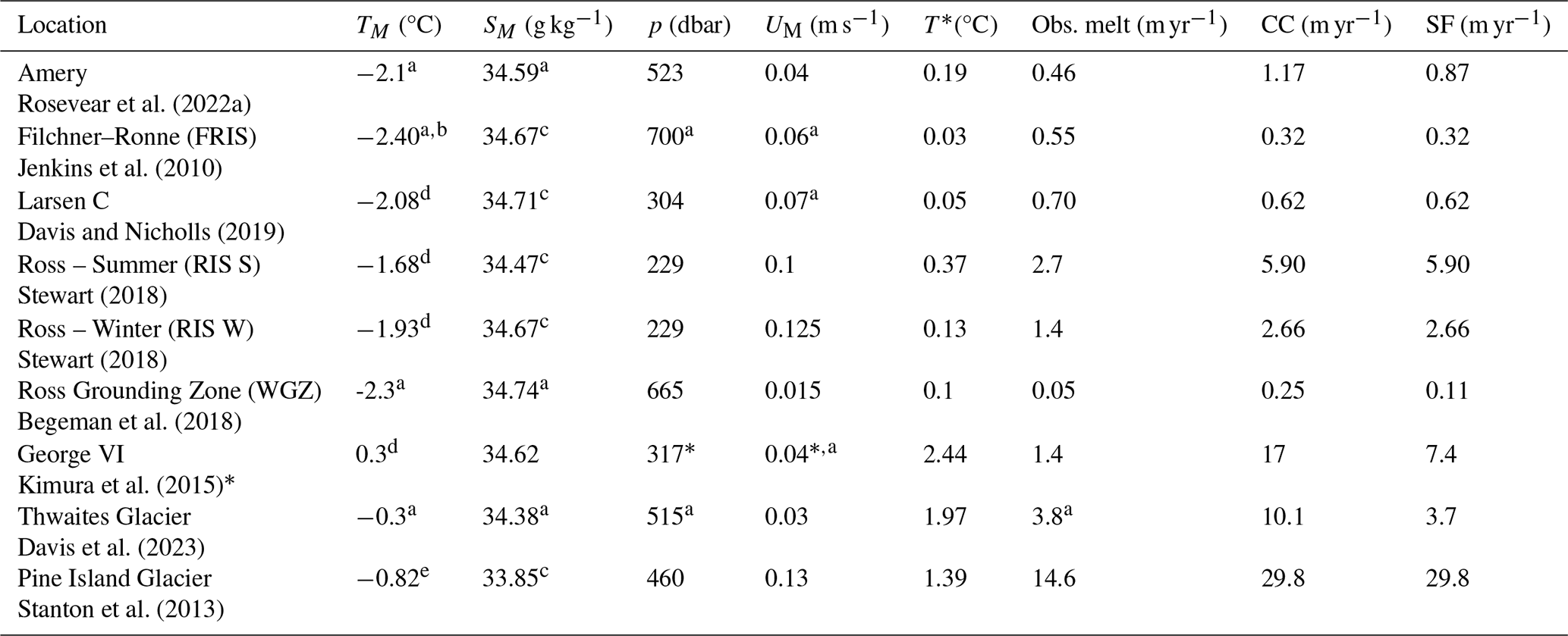
^a Values should be considered to be approximate since they are calculated from visual inspection or unclear data averaging. ^* Velocity from Middleton et al. (2022) rather than Kimura et al. (2013). ^b Converted to conservative temperature assuming the source data were reported as in situ temperature. ^c Converted from practical to absolute salinity. ^d Converted to conservative temperature assuming the source data were reported as potential temperature. ^e Far-field temperature was not provided, so this value is calculated using the freezing point equation of state to obtain the reported thermal driving. Note that friction velocities are calculated with drag coefficient C_d=0.0025 and that parameterised melt rates may differ from those stated by individual studies and Rosevear et al. (2022a) due to the use of the ConstCoeff melt parameterisation and different parameter choices including C_d. We do not perform an uncertainty analysis, but quoted uncertainties for some ice shelves are large.

Appendix C: MITgcm ISOMIP+ transects and circulation

Figure C1 is the equivalent of Fig. 4 for the MITgcm ISOMIP+ simulations.

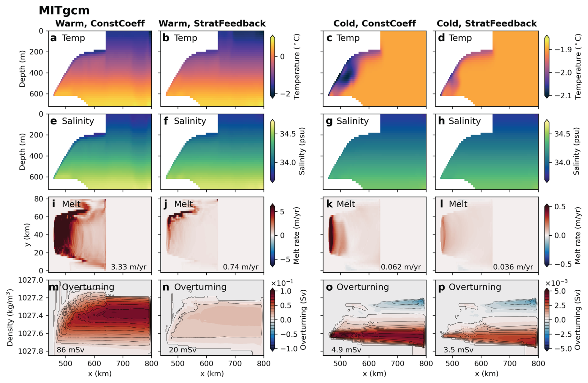
Figure C1 As in Fig. 4, for MITgcm. Temperature (a–d) and salinity (e–h) transects, melt rate distribution (i–l), and zonally averaged overturning streamfunction in density coordinates (m–p). All experiments use the ISOMIP+ protocol-specified tidal velocity U_t=0.01 m s⁻¹ as the low-velocity limit in the melt rate parameterisation. Variables are averaged over the last 180 d of the simulation, with the temperature and salinity profiles taken at the y=40 km transect. Warm experiments are in columns 1 and 2, cold in 3 and 4. Columns 1 and 3 show the constant-coefficient melt parameterisation results, and columns 2 and 4 contain the stratification feedback parameterisation. Melt rates averaged over the ice shelf are listed in panels (i)–(l). Black contours in (m)–(p) are spaced by 10 mSv in panels (m)–(n) and 0.5 mSv in panels (o)–(p), and the text lists the maximum value of the overturning streamfunction in the domain. Note the different colourbar ranges between the warm and cold simulations.

Appendix D: Pine Island Glacier melt rate distributions compared to observations

Figure D1a compares the distribution of melt rates between the three tested parameterisations, as well as melt rates computed from the Adusumilli et al. (2020a) and Zinck et al. (2024a) satellite-derived melt rate products. Whilst not directly comparable, due to different resolutions and ice shelf area due to missing data (e.g. at the grounding line, where the grounding line is taken from Morlighem et al., 2020; see Fig. D1b, c), the tuned StratFeedback parameterisation (blue colours) and StratFeedback + MK18 (yellow colours) have larger positive melt rate tails than the HJ99-neutral experiment (pink colours), more similar to the large (∼ 200 m yr⁻¹) melt rates observed near the grounding line in high-resolution satellite products (grey colours; Zinck et al., 2024a, and Shean et al., 2019). Note the two satellite products here differ significantly, highlighting the uncertainty in satellite-derived melt rates. The time periods of the satellite products and model run also differ.

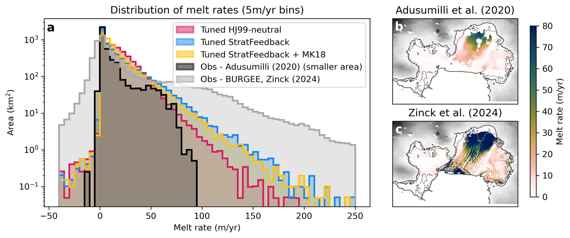
Figure D1 (a) Melt rate statistical distributions in Pine Island Glacier for the MITgcm simulation with three different basal melt parameterisations compared with Adusumilli et al. (2020a) (data: Adusumilli et al., 2020b) and Zinck et al. (2024a) (data: Zinck et al., 2024b). Note that the Adusumilli et al. (2020a) product has a coarser resolution (500 m) than the MITgcm model (200 m) and is missing data, whilst the Zinck et al. (2024a) product has a finer resolution (50 m). The y axis is logarithmically scaled. MITgcm data are averaged over simulation days 20–50. (b) Adusumilli et al. (2020a) melt rate and (c) Zinck et al. (2024a) melt rates at Pine Island Glacier with the same colourbar as Fig. 10a–c. Note, however, that it is rotated with the Antarctic Ice Sheet at the top of the figure and the ocean at the bottom. The Bedmachine V3 surface elevation (Morlighem et al., 2020) (data: Morlighem, 2022) is shown in grey, and the associated ice shelf mask is outlined with a black contour. The model domain is outlined with a dashed grey contour. Data from Adusumilli et al. (2020b) are licensed under CC BY 4.0 (https://creativecommons.org/licenses/by/4.0/, last access: 18 August 2024) and Zinck et al. (2024b) is licensed under CC BY-SA 4.0 (https://creativecommons.org/licenses/by-sa/4.0/, last access: 22 October 2024) and have been adapted in this figure.