Sensitivity of iceberg drift and deterioration simulations to input data from different ocean, sea ice and atmosphere models in the Barents Sea

Iceberg observations in the Barents Sea are scarce. Numerical simulations of iceberg drift and deterioration help fill this gap. The quality of these simulation results depends, among other factors, on the accuracy of the environmental data (e.g., wind, waves, currents, salinity, temperature), often derived from ocean, sea ice and atmosphere models. In this study, we conduct a numerical experiment simulating the drift and deterioration of a large number of synthetic icebergs. We force the iceberg model with two atmospheric reanalyses (ERA5, CARRA) and two ocean and sea ice models (Topaz, Barents-2.5) in the Barents Sea for the years 2010–2014 and 2020–2021. The differences in iceberg model output are statistically quantified, illustrated using an exemplary trajectory, and explained based on variations in environmental input. We conclude that simulation results of iceberg drift and deterioration are highly sensitive to the choice of the environmental input, depending on the simulation goal, time frame, area of interest and input characteristics. Iceberg simulations using input from Barents-2.5 yielded a distinct regional distribution of iceberg density, 8 d longer drift duration, and −6.2 × 10⁴ kg lower deterioration trend. These differences are primarily attributed to lower sea surface temperature (−0.41 °C), higher ice concentration (4 %), larger exposure to sea ice (23 %), larger water speeds (0.05 m s⁻¹) and the representation of tides and topographically-steered currents in Barents-2.5, compared to Topaz. Atmospheric input has little impact on most iceberg characteristics. However, the iceberg pathways and their southern extent remain largely insensitive to variations in environmental inputs.

1 Introduction

The Barents Sea is subject to icebergs calved from the tidewater glaciers of Svalbard, Franz-Josef-Land and Novaya Zemlya (Abramov and Tunik, 1996). The number of iceberg observations is limited due to their rare occurrence in the more navigated southwestern Barents Sea and the general sparseness of observations in the Arctic. In contrast to to Greenlandic icebergs, these icebergs are small compared to typical satellite resolutions available for observing icebergs. Statistics of iceberg occurrence therefore rely heavily on numerical simulations.

Such simulations describe the interaction of icebergs with the atmosphere, ocean and sea ice. Iceberg drift is steered by the sea water motion, waves, wind, sea ice drift, sea surface slope, coriolis forces and interaction with the sea floor (Savage, 2001). Icebergs deteriorate by wave erosion, calving, forced convection due to the differential velocities of iceberg, sea water and wind, buoyant vertical convection and solar radiation (El-Tahan et al., 1987; Savage, 2001). Previous studies (Kubat et al., 2005, 2007; Eik, 2009b, a; Keghouche et al., 2009, 2010) investigated the relative importance of those parameters and validated their model implementations with exemplary observational or experimental data. Other studies (Monteban et al., 2020; Keghouche et al., 2010) used such iceberg models to produce long-term statistics of iceberg occurrence. Eik (2009b) highlighted the influence of the environmental input and concluded that a large part of the uncertainties results from the environmental input, e.g. from ocean reanalyses.

This paper is dedicated to study the impact of varied ocean, sea ice and atmosphere input on simulations of iceberg drift and deterioration in the Barents Sea. The results aim to support the selection of environmental input for iceberg simulations to improve the accuracy of iceberg predictions and statistics in the Barents Sea. More accurate iceberg simulations will increase the safety of human operations in icy waters.

Therefore, a stat-of-the-art model for the simulation of iceberg drift and deterioration in the Barents Sea described by Monteban et al. (2020) is used herein to perform a numerical experiment. In the experiment, the iceberg model is forced by combinations of state-of-the-art ocean and atmosphere reanalyses, hindcasts and forecast systems, namely Arctic Ocean Physics Reanalysis (Topaz) (Xie, 2017b), the Barents-2.5 forecast system (MET-Norway, 2023a), the Barents-2.5 hindcast (MET-Norway, 2023c), the global atmospheric reanalysis ERA5 (Hersbach et al., 2023) and the Arctic regional reanalysis CARRA (Schyberg et al., 2023). More suitable models exist, that are not considered in this study, but could be examined in future research. Such environmental models describe the highly complex interaction of ocean and atmosphere of the Barents Sea with different resolution, model physics and representativity of the domain. The complexity of the Barents Sea arises, among other factors, from its varied bathymetry and position between warm Atlantic waters and the cold Arctic Ocean. While those differences have been characterised for ERA5 and CARRA (e.g. in Køltzow et al., 2022), the literature lacks a systematic comparison of Topaz and Barents-2.5. We statistically quantify the differences between the environmental models for the Barents Sea over the years 2010–2014 and 2020–2021. This detailed and case-specific knowledge is extracted from model descriptions and quality information from literature. This novel combination of knowledge about the differences in ocean, sea ice and atmosphere variables is used in the core of this study to examine the effects of these differences on iceberg drift and deterioration simulations in the Barents Sea.

The iceberg drift and deterioration simulations are performed for a large number of simulated synthetic icebergs in the Barents Sea. The simulation results with varied environmental input are compared statistically with respect to various characteristics of the simulated iceberg trajectories, i.e. iceberg deterioration, iceberg drift (Sect. 4.1) and resulting distribution in the domain (Sect. 4.2, 4.3). Further, we examine one synthetic iceberg trajectory to illustrate the statistical results (Sect. 4.4). In the discussion (Sect. 5), the differences between the simulations with varied environmental input are traced back to the differences between the ocean, sea ice and atmosphere models, that we quantify in Sect. 3. We further discuss the suitability of the environmental datasets in different applications of iceberg simulations (Sect. 5.2).

We emphasise that this study focuses on the impact of the choice of environmental input data on iceberg statistics rather than an analyses of the absolute iceberg statistics. We refrain from analysing the impact of iceberg model settings on iceberg statistics and inherit the iceberg model settings from Monteban et al. (2020). We do not compare to observations of iceberg trajectories, as we choose a purely statistic approach and observations are scarce.

2 Description of the Experiment

A numerical experiment is conducted in which an iceberg drift and deterioration model (Monteban et al., 2020) is forced by different combinations of ocean, sea ice and atmosphere datasets to assess the impact of varying environmental input. This Section provides an overview of the experiment and the iceberg model.

2.1 Experiment setup

The iceberg model is forced by four combinations of the ocean, sea ice and atmosphere data. The combinations are (i) the reference case using the global models Topaz and ERA5 (12.4 and 31 km horizontal resolution), (ii) the high-resolution, regional simulation case using Barents-2.5 and CARRA (both 2.5 km). The combinations Topaz and CARRA (12.4 and 2.5 km) and Barents-2.5 and ERA5 (2.5 and 31 km) serve to estimate the individual influence of ocean, sea ice and atmosphere input on the simulations results. We did not conduct a full sensitivity analysis, varying every variable individually, to avoid physically inconsistent input (of e.g. SST and CI) and to resemble a probable use case as closely as possible. The simulations are performed for the years 2010–2014 and 2020–2021, which were the only years all environmental datasets were available at the time the simulations were performed. Despite the small number of years included and large interannual variability, we characterise the two most recent decades with sea ice regimes at different stages of the advancing climate change. Future studies may concern themselves with analysing the newly available, extended time period.

2.2 Iceberg seeding

Following the seeding procedure in Monteban et al. (2020), icebergs are seeded near the tidewater glaciers of Franz-Josef-Land, Austfonna, Edgeøya and Novaya Zemlya (Fig. 1) from July to November of the years 2010–2014 and 2020–2021. The iceberg length is sampled from a generalised extreme value (GEV) distribution. The minimum initial iceberg length is set at 34 m, corresponding to the maximum resolution of the satellite observations and the definition of a bergy bit (10 m height). The iceberg width and height are derived from empirical relations described by Dezecot and Eik (2015). The set of seeded icebergs is representative of the domain, as the size and number of seeded icebergs are based on satellite observations near the glaciers (Monteban et al., 2020). A meaningful statistic is ensured by a randomised seeding day, location and length within this observed range, thus exposing them to a random selection of environmental conditions. These initial settings vary for all released icebergs but are identical for simulations with varied environmental input. Note that the seeding locations are far enough to the coastline to avoid grounding during the initial phase of the simulations.

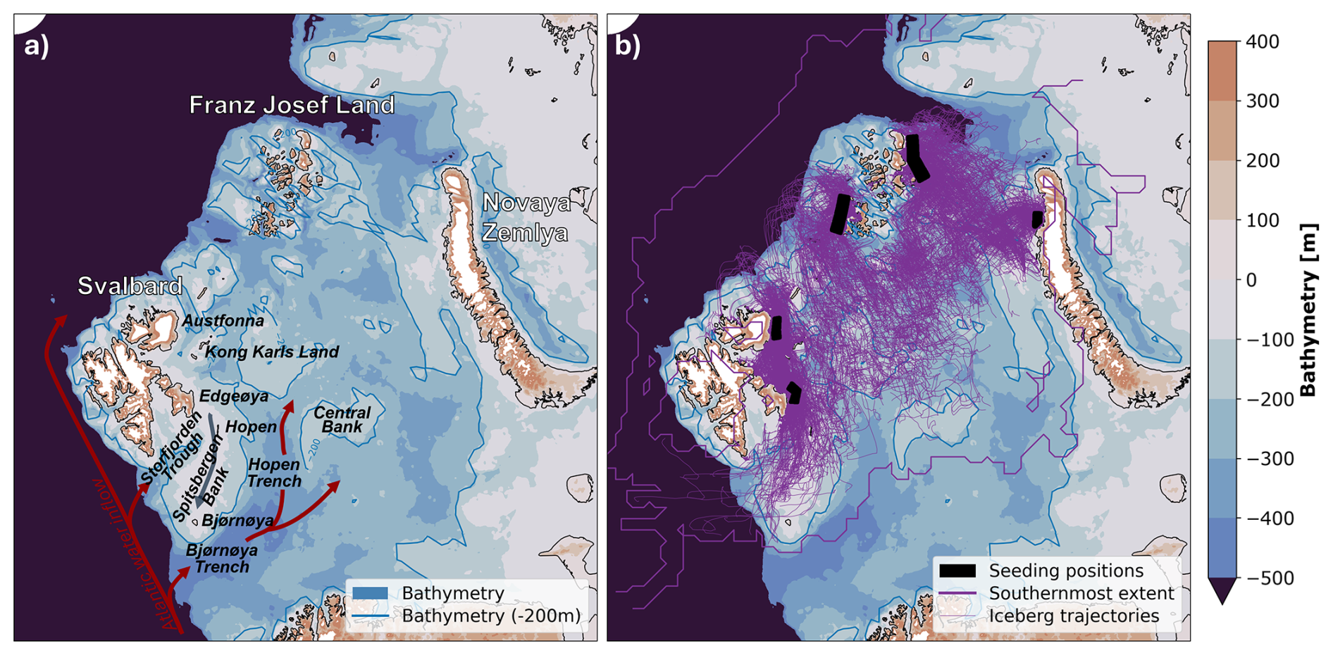
Figure 1 Map of the Barents Sea (a) and main simulated iceberg pathways (b) with seeding regions (black areas), the maximum simulated iceberg extent (thick purple lines) and an exemplary subset of the trajectories (thin purple lines).

2.3 Model for iceberg drift and deterioration

The numerical model for the simulation of iceberg drift and deterioration and its settings is adopted from Monteban et al. (2020). The iceberg model is Lagrangian and deterministic. The iceberg drift is simulated based on wind, sea water velocity, sea ice drift, the resulting Coriolis force and interaction with the sea floor. The pressure gradient and Coriolis forces are included under the assumption of geostrophic balance. Wave forces are included by calibrating the wind drag coefficient implicitly. The iceberg drift categorises “light” sea ice (CI >15 %) and “heavy” sea ice (CI ≥90 % and $h_{\mathrm{si}}\ge h_{\min }=\frac{\mathrm{13}\mathrm{000}}{\mathrm{20}\mathrm{000}\cdot \exp (-\mathrm{20}(\mathrm{1}-\mathrm{CI}\left)\right)}$) and neglects sea ice outside the sea ice edge (CI ≤15 %). Note that heavy sea ice is assumed under the simultaneous occurrence of high CI and sufficient sea ice strength. Sea ice strength is described by the thickness threshold h_min, which is derived from an empirical relation of CI (Lichey and Hellmer, 2001). The added mass is set to zero. The iceberg melt is a function of basal turbulent melt, vertical thermal buoyant convective melt and wave erosion based on wind, water velocity and the sea surface temperature. The wave erosion term disregards swell waves due to simulated small iceberg sizes but includes local wind waves as function of wind and water velocity. Melt by solar radiation is neglected due to its minor influence in the far north and calving is not explicitly modelled. The drift and deterioration equations and model parameters can be found in (Monteban et al., 2020).

The iceberg model solves the drift and deterioration equations at 2-hourly time steps and updates iceberg position, size and velocity. The simulation is stopped when the iceberg has melted to the size of a growler (H≤10 m), leaves the simulation domain or when the desired simulation period is exceeded.

The iceberg model is driven by environmental data from the present or most recent time step and the nearest grid cell of the respective environmental dataset without interpolation. When no data is available in the nearest grid cell, we also consider surrounding grid cells at larger distance to the iceberg for better coverage of coastal regions. As the environmental datasets have different grids and resolutions, the input data is not necessarily taken from the same geographical area for the same iceberg position. In spite of the availability of more sophisticated model equations and assimilation methods, the described iceberg model exhibited its robustness in Monteban et al. (2020) and is herein used without further evaluation of the model settings' impact on the simulation results.

3 Analysis of ocean, sea ice and atmosphere data in the iceberg pathways

This study uses 10 m wind (v_a) from ERA5 (Hersbach et al., 2023) and CARRA (Schyberg et al., 2023). The sea surface velocity (v_w), sea surface temperature (SST), sea ice concentration (CI), ice thickness (h_si), and ice drift velocity (v_si) are obtained from Topaz (Xie, 2017b) and Barents-2.5 (hindcast 2010–2014, forecast 2020–2021) (MET-Norway, 2023a, c). Table 1 provides an overview of the environmental models. All data is used at its original spatial resolution. In this study, we introduce the term iceberg pathways to refer to all regions and time periods in which icebergs were simulated. Figure 1 depicts the spatial occurrence of icebergs in the Barents Sea. We analyse environmental data in the pathways, specifically environmental model grid cells and model time steps that contributed to the iceberg simulations. Figure 2 compares the environmental variables in the iceberg pathways in Fig. 2 and Table 2 and relates the differences to known model uncertainties.

Xie (2017b)MET-Norway (2023c, a, b)Hersbach et al. (2023)Schyberg et al. (2023)Sakov et al. (2012)Röhrs et al. (2023)Fritzner et al. (2019)Hersbach et al. (2020)Køltzow et al. (2019)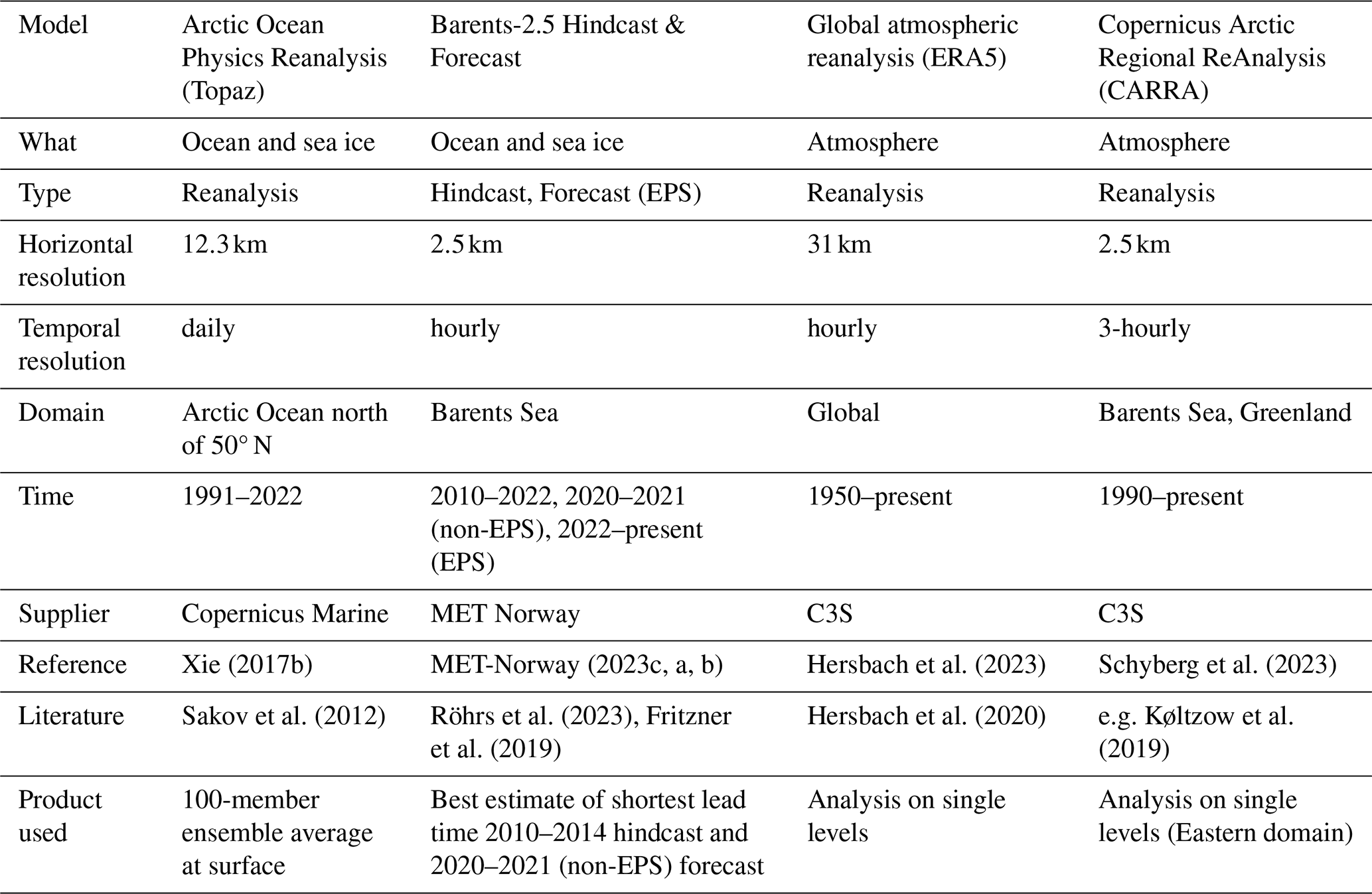

Table 1 Overview of ocean, sea ice and atmosphere models.

3.1 Sea surface temperature

We compare the SST in Topaz and Barents-2.5 and find that it is 0.41 °C lower for the iceberg pathways in Barents-2.5. The spatial differences follow the bathymetry and sea ice characteristics (Table 2, Fig. 2). The largest differences can be seen along the inflow of warm Atlantic waters into the West Spitsbergen Current and the Barents Sea (e.g. into the Storfjorden Trough, Bjørnøya Trough and Hopen Trench), and along the spring sea ice edge. In the literature, Topaz is known to have a large positive SST bias in those regions due to issues with simulating the circulation of Atlantic water inflow and the topographic steering (Xie et al., 2017a). Barents-2.5 is known to have a negative SST bias and large SST mismatches in the marginal ice zone (Röhrs et al., 2023) due to two-way coupling between the model ocean and sea ice component. Topaz is described as closer to the observations than the Barents-2.5 hindcast (Idžanović et al., 2024). Note that Fig. 2 presents the difference in sea ice variables between Topaz and Barents-2.5, calculated as CI(Topaz) − CI(Barents2.5) within the maximum modelled sea ice extent, including areas where sea ice is present only in one of the models and during limited time periods.

Table 2 Statistics of ocean, sea ice and atmosphere variables in Topaz and Barents-2.5, ERA5 and CARRA for the simulated iceberg pathways in the Barents Sea (spatial grid cells and time steps used in the iceberg simulations). The variables are sea surface temperature (SST), sea surface speed (v_w), sea ice concentration (CI), sea ice thickness (h_si), sea ice drift speed (v_si) and 10m wind speed (v_a). ∅ denotes the variable average and p represents the proportion of iceberg simulation time steps during which specific characteristics (e.g. CI >15 %) are observed. Time steps and grid cells in which the variable does not influence iceberg drift and deterioration (e.g. heavy sea ice conditions for v_w) are excluded. The values for v_a are given for the iceberg pathways as simulated by different ocean and sea ice (a) or atmospheric (b) input.

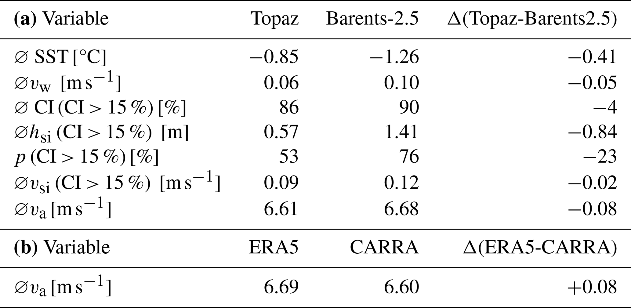
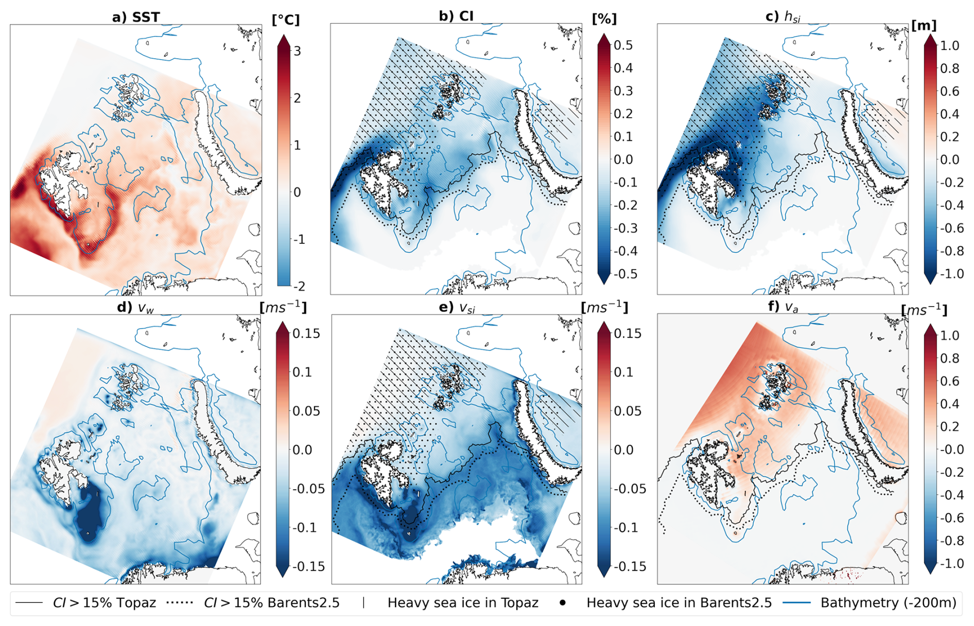
Figure 2 Spatial differences in ocean, sea ice and atmosphere variables in the Barents Sea in Topaz, Barents-2.5, ERA5, and CARRA, namely (a) SST, (b) CI, (c) h_si, and total speeds of (d) v_w, (e) v_si, and (f) v_a. Shown for comparison, the −200 m bathymetry isolines (blue lines), the average April sea ice edge (CI > 15 %, black lines), and the extent of heavy sea ice (CI ≥90 %, h_si≥h_min, hatches) for 2010–2014 and 2020–2021.

3.2 Sea ice

We find that CI and h_si are on average 4 % and 0.84 m larger in Barents-2.5, compared to Topaz, within the sea ice edge (CI >15 %) in the iceberg pathways (Table 2). Some of the largest differences between the sea ice models are present along the typical spring sea ice edge, especially around northern Svalbard (Fig. 2). Sea ice (CI >15 %) also occurs in 23% more time steps in the iceberg pathways in Barents-2.5 as the southward extent of light and heavy sea ice is larger. Previous studies describe an underestimation of sea ice area, CI and h_si (especially along the sea ice edge) in Topaz (Xie et al., 2017a; Xie and Bertino, 2022) and general overestimation, but skilful CI, in Barents-2.5 (Röhrs et al., 2023). Topaz CI is found to be closer to the observations as the Barents-2.5 hindcast (Idžanović et al., 2024). Further analysis in this study (not shown) revealed large differences between the sea ice variables in Barents-2.5 forecast (used 2020–2021), which is constrained to sea ice observations, and the Barents-2.5 hindcast (used 2010–2014), which is a free-run. Further analysis (not shown) also revealed that the SST and sea ice differences vary seasonally. Compared to the known too fast decline and freeze-up in Topaz (Xie et al., 2017a; Xie and Bertino, 2022), we found that the melt season is delayed and the sea ice advance is similar in Barents-2.5.

3.3 Ocean and sea ice velocity

The sea surface and sea ice speeds are on average 0.05 and 0.02 m s⁻¹ faster over the iceberg pathways in Barents-2.5 (Table 2, Fig. 2). The v_w differences are particularly large in coastal and shallow areas (between Svalbard and Franz-Josef-Land, around Svalbard, Spitsbergen Bank, and Central Bank). The differences are smaller in open ocean. The v_si differences are largest around the sea ice edge (CI ≈15 %) and south-western Svalbard. In contrast, Topaz has faster water and sea ice speeds towards the Eurasian Basin. In contrast to Topaz, Barents-2.5 accounts for the effects of air pressure and tides on the water velocity, and represents local water velocities due to its high horizontal and temporal resolution. Model skill varies over time and spatial scales and the predictive skill for surface water speed and direction in Barents-2.5 is low. Some skill can be accounted to water velocities in mainly wind-driven conditions, and the sea ice velocity. The water and sea ice speeds have a positive bias (Röhrs et al., 2023b; Idžanović et al., 2023). Lower horizontal resolution ocean models, such as Topaz, have smaller gradients and lower velocities in general. Topaz also shows issues with simulating the circulation of Atlantic water inflow and the topographically-steered currents. Note that, in Table 2 and Fig. 2, the diurnal tidal cycle largely cancels out in the water velocity average and its difference in Topaz and Barents-2.5. However, Fig. 2 still shows the differences due to other processes (e.g. topographically-steered currents). Further analysis (not shown) confirmed large differences for hourly time steps in shallow areas such as Spitsbergen Bank) due to tidal representation.

3.4 10 m Wind

In the iceberg pathways of the Barents Sea, the average wind speed difference between ERA5 and CARRA (+0.08 m s⁻¹) is relatively small compared to the absolute wind speeds (∅ 6.60 to 6.69 m s⁻¹) and varies just as much between the two atmospheric models as between the pathways caused by varied ocean and sea ice input. Differences are especially small over open waters and are locally larger along the coastlines with complex topography. In previous studies, CARRA was found to provide added value over ERA5, especially over complex topography and sea ice, due to its improved physical parametrisation and higher resolution satellite observations of sea ice (Køltzow et al., 2019, 2022; ECMWF, 2024). We highlight larger average wind speeds in ERA5 in the northern, frequently sea-ice-covered part of the domain and larger speeds in CARRA in the southern, water-covered part of the domain in Fig. 2, that are likely due to different representation of surface roughness over water and sea ice, or prescription of different CI products (Hersbach et al., 2020; Yang et al., 2020; ECMWF, 2024).

We highlight that similarities (e.g. in ERA5 and CARRA wind) partly result from the interconnection of the described environmental models by the use of the respective other models (or different version of a similar setup) at the ocean, sea ice and atmosphere interface and the lateral boundaries (e.g. CARRA using ERA5 at lateral boundary and surface or Topaz using ERA5 at the surface). Unrelated atmospheric models may exhibit larger differences.

4 Analysis of the iceberg simulation results

4.1 Iceberg drift and deterioration

In this section, we compare the distance along the trajectory (Track), the shortest distance between seeding and the melt position (Effective) and the time an iceberg persists until it is melted (Duration). Further we analyse the relative contributions of the various melt terms.

The total iceberg deterioration rate of an iceberg in simulation time step j (with length d$t=\mathrm{3600}\cdot \mathrm{2}\mathrm{s}$) is calculated as mass loss or reduction in volume multiplied by the density ρ_i of glacial ice (Eq. 1).

$$\begin{array}{}\text{(1)}& {\displaystyle }{\mathit{\delta }}_j=m_{j+\mathrm{1}}-m_j={\mathit{\rho }}_{\mathrm{i}}\cdot (H_{j+\mathrm{1}}\cdot W_{j+\mathrm{1}}\cdot L_{j+\mathrm{1}}-H_j\cdot W_j\cdot L_j)\text{(2)}& {\displaystyle }={\mathit{\rho }}_{\mathrm{i}}\cdot \left(\right[H_j+\mathrm{\Delta }{H}_j]\cdot [W_j+\mathrm{\Delta }{L}_j]\cdot [L_j+\mathrm{\Delta }{L}_j]-H_j\cdot W_j\cdot L_j)\end{array}$$

where $\mathrm{\Delta }{H}_j=M_{\mathrm{fw}}\cdot \mathrm{d}t$ is the reduction in height during time step due to melt at the base (M_fw). $\mathrm{\Delta }{L}_j=\mathrm{\Delta }{W}_j=(M_{\mathrm{e}}+M_{\mathrm{v}})\cdot \mathrm{d}t$ is the reduction at the sides due to wave erosion (M_e) and vertical buoyant convection (M_v). Equation (3) introduces the contribution of each melt term relative to the total deterioration (δ(term), in %). i and j are counters of icebergs and time steps, respectively. I and J are the total number of simulated icebergs and time steps, respectively.

$$\begin{array}{}\text{(3)}& \mathit{\delta }\left(\mathrm{term}\right)={\displaystyle \frac{{\sum }_{i=\mathrm{1}}^I{\sum }_{j=\mathrm{1}}^J\mathit{\delta }(i,j,\mathrm{term})}{{\sum }_{i=\mathrm{1}}^I{\sum }_{j=\mathrm{1}}^J\mathit{\delta }(i,j)}}\cdot \mathrm{100}\mathrm{\%}\end{array}$$

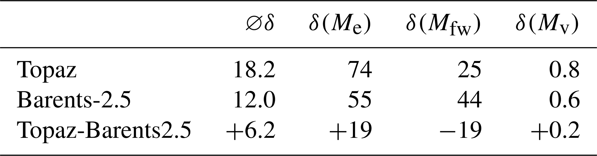
Wave erosion δ(M_e) contributes most (55 %–74 %), followed by basal melt δ(M_fw) (25 %–44 %) (Table 3). However, the relative importance of the deterioration terms varies with the environmental data. Comparing the simulations with different environmental input, icebergs with Topaz input have larger wave erosion (+19 %) and smaller basal melt (−19 %). The relative contribution in vertical convection δ(M_v) and its difference with environmental input is small. The average iceberg mass loss (from simulation start to end) is larger in simulations with Topaz input (+6.2 × 10⁴ kg). Further studies (not shown) indicated small melt rates for times steps in sea ice. An example of the relative contributions of the deterioration terms and their differences for simulations with different environmental input is given in Sect. 4.4.

Table 3 Total iceberg deterioration and the contribution from different deterioration terms (wave erosion M_e, basal melt M_fw and vertical buoyant convection M_v) in simulations using Topaz and Barents-2.5, and their difference. The values are expressed as average total deterioration (∅δ, in 10⁴ kg) and relative contribution to the total mass loss or deterioration (δ(M,%)). Note that δ(M_v) is given with higher precision to show its difference with ocean input.

In simulations with different ocean and sea ice inputs, icebergs with Topaz input drift on average 8 d shorter, 18 km less in distance along the track, but 6 km more in effective distance (Fig. 3). These differences are partly relevant as they make up 28 %, 5 % and 6 % of the mean absolute values of all simulations. The difference between simulations with varying atmospheric input are minor.

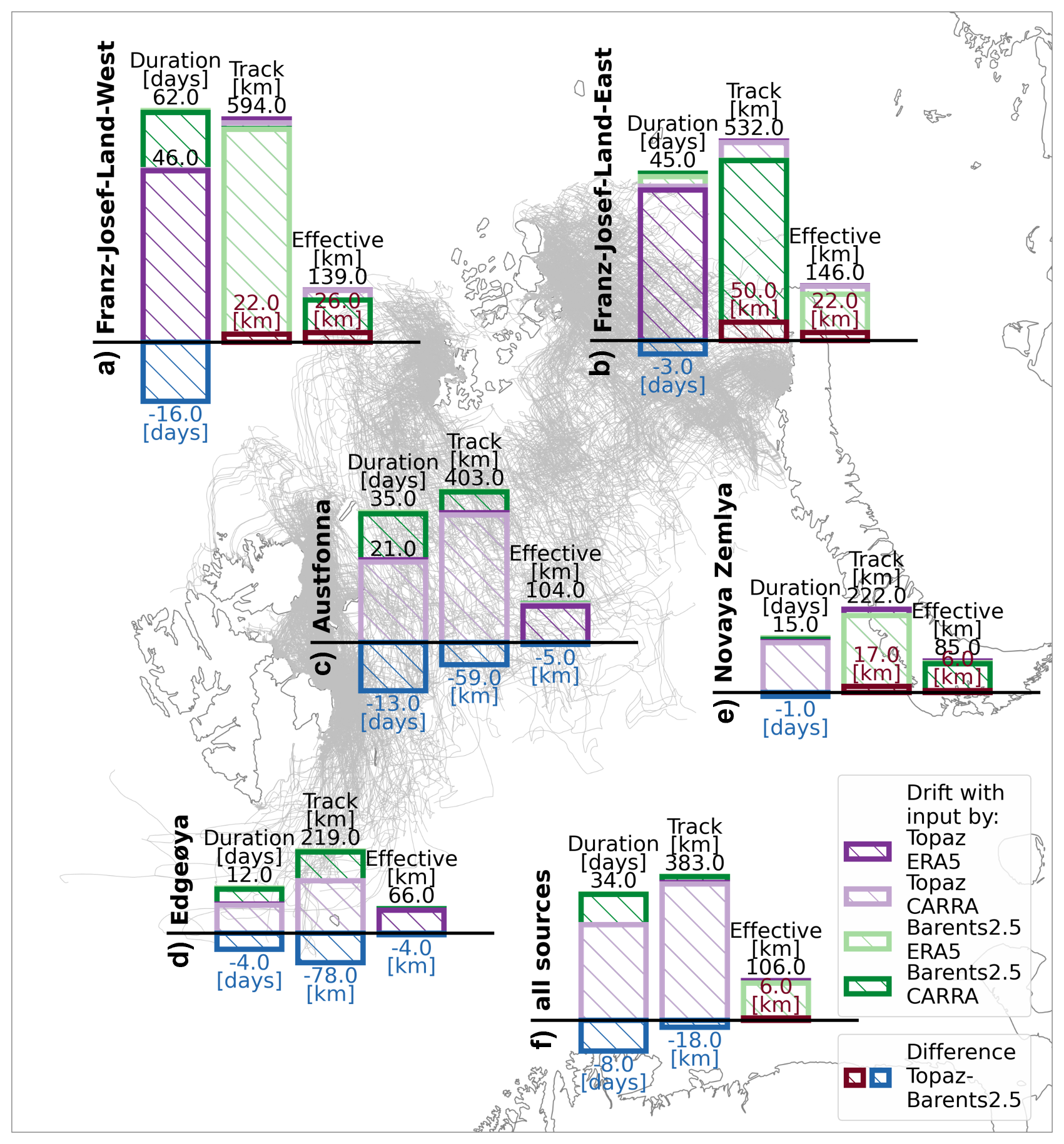
Figure 3 Average drift duration [days], distance (Track, Effective) [km] for icebergs originating from the sources Franz-Josef-Land West and East (a, b), Austfonna (c), Edgeøya (d) and Novaya Zemlya (e), and their combination (f). Drift statistics are given for simulations using different environmental input (green and purple bars) and their difference (red and blue bars)

The iceberg drift duration and distance also vary by source, and its seeding characteristics (number and size) (Fig. 3). The dependency on the seeding location causes a variation of 8 to 62 d, 140 to 594 km (Track) and 61 to 146 km (Effective). Iceberg drift duration and distances (Track, Effective) are highest for icebergs originating from Franz-Josef-Land and Austfonna, and smaller for Edgeøya and Novaya Zemlya in all simulations.

Analysing the dependency on both source and environmental input, the differences between the sources is larger than the difference due to the environmental input (Fig. 3). Similarities and differences in iceberg drift from various sources are largely reproduced by the simulations with different environmental input. However, differences between drift under Topaz and Barents-2.5 input are significant and vary in both positive and negative magnitudes. For example, icebergs with Topaz input from Franz-Josef-Land drift on average larger distances, but in a shorter duration.

4.2 Spatial iceberg density

Iceberg density is a measure of the average number of icebergs in a domain over a time period, along with the number of simultaneous occurrences. The iceberg density is derived from the number of icebergs i that are within a defined grid cell at the same simulation time step, the number of time steps n in which i icebergs are within the same grid cell and the total number of simulation time steps J. The probability of having i icebergs in one grid cell at same time step p(i) is calculated for every iceberg i by Eq. (4). The areal density ρ_a (referred to as iceberg density hereafter) is given by Eq. (5) with the surface area of the grid cell A_grid cell. The unit of ρ_a is “number of icebergs per area and time step”. In this analysis, iceberg density is aggregated on an artificial grid of 25 km horizontal resolution, similar to a curvi-linear Topaz grid at reduced resolution. Apparent iceberg occurrences on land result from accumulating occurrences on this grid.

$$\begin{array}{}\text{(4)}& {\displaystyle }p\left(i\right)={\displaystyle \frac{n\left(i\right)}{J}}\text{(5)}& {\displaystyle }{\mathit{\rho }}_{\mathrm{a}}={\displaystyle \frac{{\sum }_{i=\mathrm{0}}^{\mathrm{\infty }}i\cdot p\left(i\right)}{A_{\mathrm{grid}\mathrm{cell}}}}\end{array}$$

Figure 4 shows maps of the iceberg density in the Barents Sea for the simulations with different environmental input. Iceberg densities are highest around eastern Svalbard, Franz-Josef-Land and northwestern Novaya Zemlya and decreases with increasing distance to those locations.

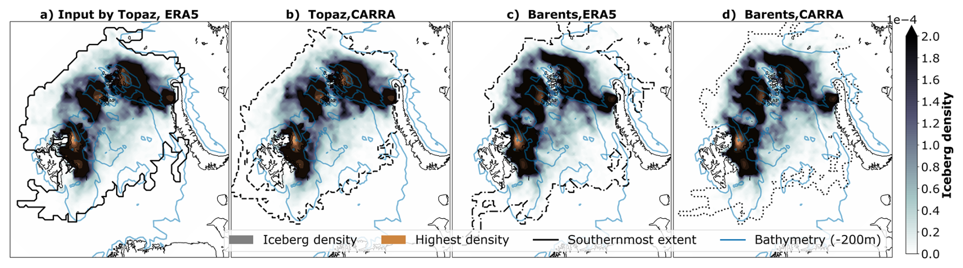
Figure 4 Iceberg density (colours) and southernmost extend (black line), aggregated from simulations using (a) Topaz and ERA5, (b) Topaz and CARRA, (c) Barents-2.5 and ERA5 and (d) Barents-2.5 and CARRA. Highest densities are highlighted in orange colour.

Figure 5 shows the spatial density differences between the simulations with different environmental input. Density differences are as large as absolute densities, which is highlighted by similar density range in Figs. 4 and 5. Deviations by varied ocean and sea ice input are larger than deviations by varied atmospheric input, however some effects of ocean and atmospheric input add up while some cancel each other out.

Simulations of varied ocean and sea ice input show significant difference in large parts of the domain, and especially around Svalbard and Franz-Josef-Land (Fig. 5). Thereby, simulations with Topaz input have higher density near the coastline of Franz-Josef-Land and Svalbard, and lower density farther from the archipelagos. The density differences are decreasing towards the open ocean. We also highlight the larger density for simulations with Barents-2.5 input in the northernmost parts of the domain, and the higher density to the northwest (northeast) of Bjørnøya for simulations with Topaz (Barents-2.5) input. Density differences due to atmospheric input are small across most of the domain, but can be in the scale of the absolute values regionally.

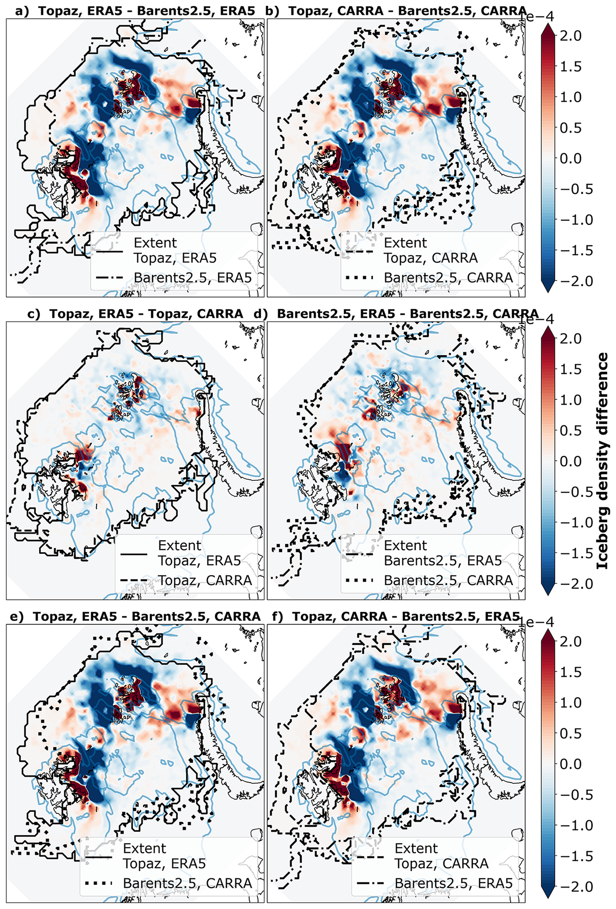
Figure 5 Difference of iceberg density (colours) and southernmost extend (lines) in simulations with (a, b) varied ocean and sea ice input, (c, d) varied atmospheric input and (e, f) variations of both environmental inputs.

4.3 Spatial and seasonal iceberg extent

The iceberg extent is a measure of how far icebergs drift, how much they spread and how much they are restricted to common pathways. The maximum spatial iceberg extent is indicated by the black lines in the Figs. 4 and 5 and shows little difference across varied environmental input.

More detailed analysis (not shown) indicates that the southernmost iceberg trajectories reach south of Bjørnøya and to the south-eastern Barents Sea around 72–74° N, regardless of the environmental input. Some of these icebergs drift within sea ice of high concentration, while others drift in open waters. The southernmost trajectory reached 72° N in the Central Basin for simulations with Barents-2.5 input, as described in Sect. 4.4.

We adopt and modify the definition of the iceberg extension from Keghouche et al. (2010) and show the relative number of grid cells containing icebergs at a given time in Fig. 6. The iceberg extension varies with time and between the simulations with different environmental input. The iceberg extension varies in simulations with both different atmospheric and ocean-sea ice input, and at the same amplitude.

In detail, the iceberg extension follows a seasonal cycle and exhibits multi-year variability (Fig. 6). This variability is visible in all simulations with different environmental input, although with small deviations. The iceberg extension increases from July to December, when icebergs are seeded, and then decreases again until July. The period from July to December is characterised by large deviations with varied ocean input and small variations with atmospheric input. Largest differences with varied ocean and sea ice input occur from August to September and November to December. The period from December to June shows similar deviations with varied ocean and atmospheric input. These deviations are differently pronounced in individual years of the time series.

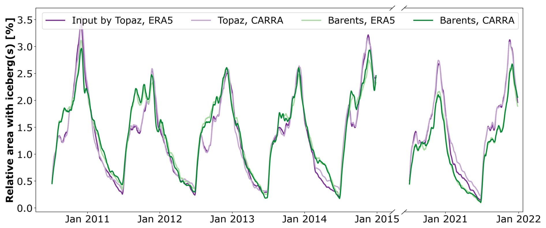
Figure 6 Time series of iceberg extension in the iceberg simulations with different environmental input (colours) from 2010 to 2014 and 2020 to 2021. The extension is relative to the number of artificial analysis grid cells with a horizontal resolution of 25 km. A 10 d rolling average is applied.

4.4 Example of an iceberg trajectory

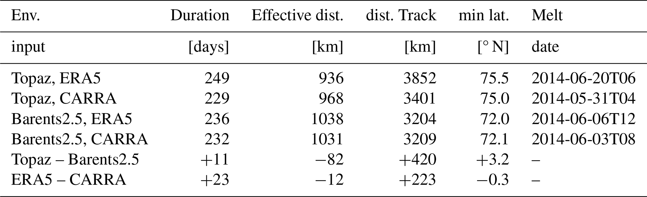
This Section presents an illustrative example of the drift and deterioration of the synthetic iceberg, referred to as iceberg 2013-788. The trajectory of iceberg 2013-788 is one of the longest (up to 249 d, 1030 km effective and 3900 km track distance) and southernmost trajectories (down to 72° N) amongst the statistics of 72 884 simulated trajectories discussed in this study (Table 4). The exceptionally long drift is caused by an above average initial size and initial position far north. As such, the example is not suitable for explaining the average differences in iceberg simulations with varied environmental input, but serves as illustration of the impact of environmental input.

The iceberg drifted southward from Franz-Josef-Land between autumn 2013 to spring 2014 (Fig.7). Trajectories with different ocean and sea ice input deviate significantly in the second half of the drift, leading into the Central Basin under Barents-2.5 input and into the Hopen Trench under Topaz input. The icebergs with Barents-2.5 input drifted 3° further south (Table 4). The trajectories with Topaz input have a longer drift duration (+11 d) and distance along the track (+420 km), but a shorter effective drift distance (−82 km). The trajectories show minor deviations due to varied atmospheric input.

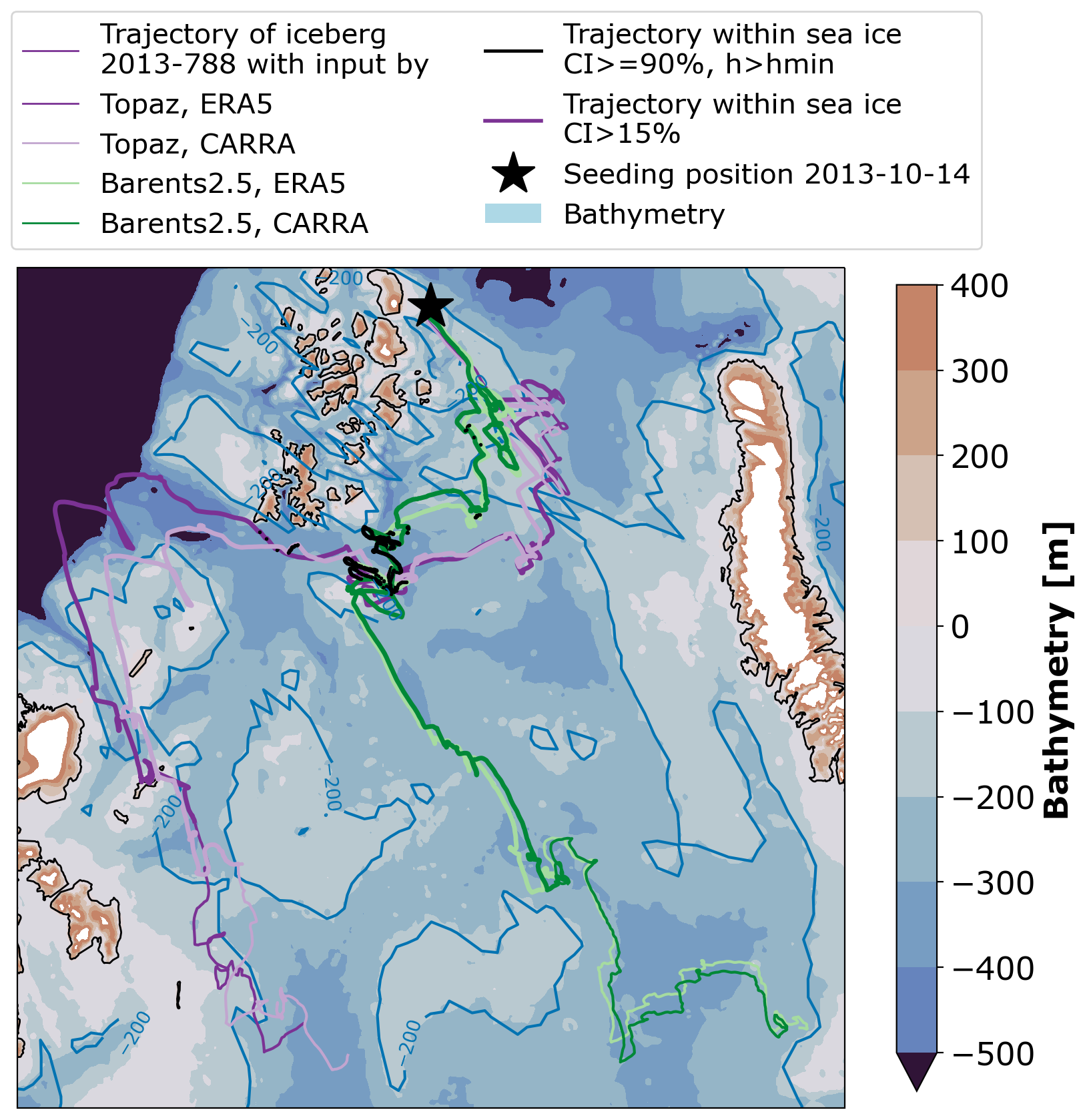
Figure 7 Simulated drift of iceberg 2013-788, seeded at the 14 October 2013, close to north-eastern Franz-Josef-Land (star). The trajectories correspond to simulations of iceberg drift and deterioration with varied environmental input (coloured lines). Along the trajectories, simulation time steps in light sea ice (CI >15 %, thicker lines) and heavy sea ice conditions (CI ≤90 % and h_si>h_min, black lines) are marked.

Table 4 Characteristics of the drift of iceberg 2013-788. Iceberg drift duration [days], effective drift distance [km], drift distance along the trajectory [Track, km], southern-most latitude [min lat. ° N] and simulation end date (Melt date).

The environmental conditions in the Barents Sea are shown for selected time steps during the winter 2013–2014 in Fig. 8. The environmental input along the trajectory of iceberg 2013-788 is shown as timeseries in Fig. 9.

At the seeding time in mid-October 2013, sea ice (CI >15 %) is restricted to the north and west of Franz-Josef-Land in Topaz. At the same time, sea ice in Barents-2.5 encloses the archipelago, setting the iceberg in light sea ice conditions (black line in Fig. 8). During the winter, the sea ice expands south-east-ward, with light sea ice reaching as far south as Hopen island for Topaz and as far south as Bjørnøya for Barents-2.5 in late April. The cover of heavy sea ice is larger in Barents-2.5 throughout the winter (Fig. 8, point hatches). The sea surface temperature reflects this difference in the spatial distribution accordingly.

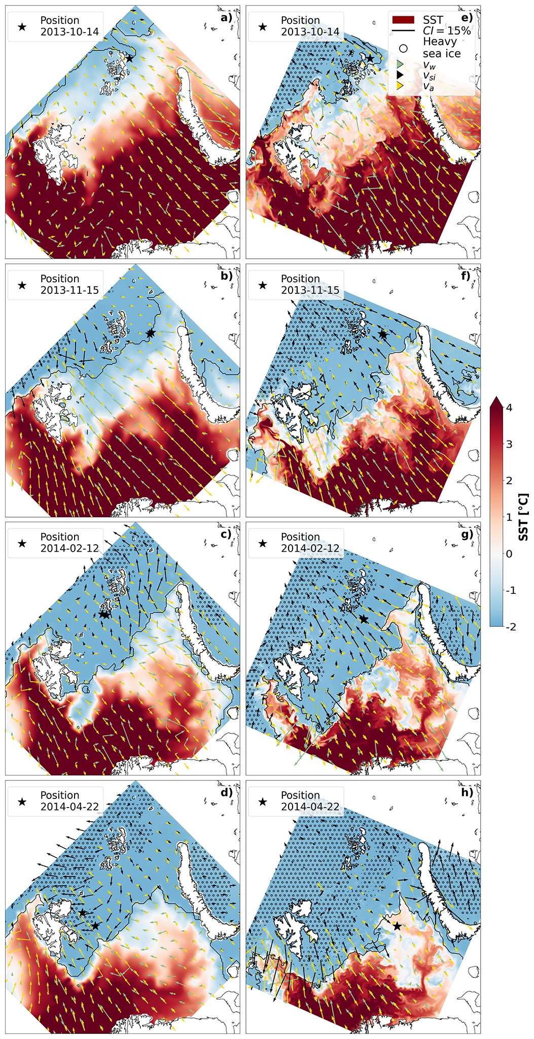
Figure 8 Environmental conditions in the Barents Sea at the 14 October 2013 (a, e), 15 November 2013 (b, f), 12 February 2014 (c, g) and 22 April 2014 (d, h). Ocean and sea ice conditions are provided by Topaz (a–d) and Barents-2.5 (e–h). The atmospheric conditions are provided by ERA5 (a–d) and CARRA (e–h). Shown variables are the sea surface temperature (contour colours), sea ice edge (CI >15 %, black line), heavy sea ice (CI $\le \mathrm{90}\mathit{\%},h_{\mathrm{si}}>h_{\min }$, hatches), as well as momentary sea ice drift (black arrows), sea surface velocity (green arrows) and 10 m-wind (yellow arrows). Note that the directional data is given for reduced (approx. 100 km) resolution for increased visibility. The respective simulated position of iceberg 2013-788 is marked by black stars.

Along the trajectory, the icebergs drift within the sea ice edge 70 %–77 % of the simulation days (Table 5, Fig. 9). Simulations with Barents-2.5 input show a larger number of days with sea ice (+7 % of days), average 10 % larger CI and 0.1 m larger h_si. The SST is on average 0.01 °C warmer in trajectories with Topaz input (Table 5). The SST along the trajectory is characterised by the present sea ice until April/May 2014 (≈ −2 °C) and followed by the drift into warmer Atlantic waters (up to +4 °C) in the Hopen Trench and the Central Basin (Figs. 7, 9).

We highlight the period between 1 April and 15 May 2014, when the icebergs drift out of the sea ice edge, to the east of Svalbard (Topaz input) and in the Central Basin (Barents-2.5 input). The general environmental situation in April 2013 can be described by the yearly maximum sea ice extent and infusions of warm Atlantic waters towards the sea ice edge (e.g. along the Hopen Trench and Central Basin) (Fig. 8). Along the trajectories, the icebergs face decreasing sea ice concentration and thickness and increasing SST during their southward drift (Fig. 9). The icebergs also face rapid changes in wind and water speed.

Wind, sea water and sea ice speed vary across the domain and fluctuate on short temporal scales in the timeseries, especially for Barents-2.5, ERA5 and CARRA (Fig. 9). Further analysis (not shown) obtained that the wind speed varies less between the atmospheric input than between the trajectories caused by varied ocean input.

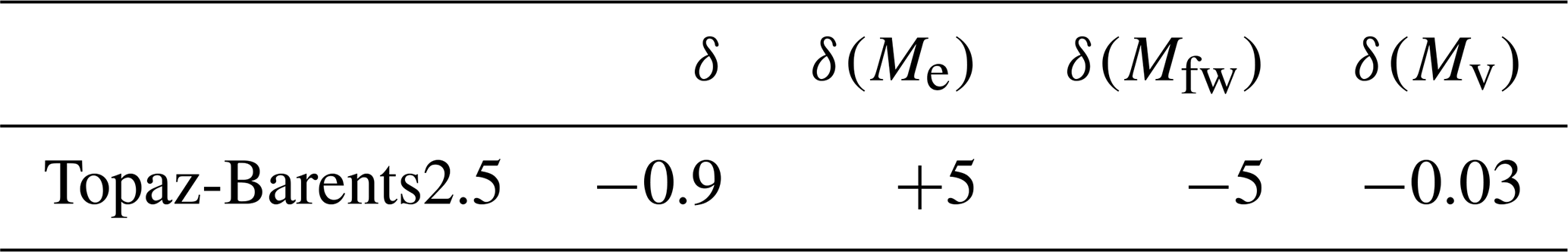
The iceberg deterioration rate is small (20×10⁴ kg 2 h⁻¹) during the drift within sea ice, and basal melt dominates (Fig. 9, means not shown). When the icebergs start to drift outside of the sea ice, the deterioration rates increase (89.5×10⁴ kg 2 h⁻¹) and the contribution by wave erosion dominates (not shown). Note that the deterioration rate decreases with decreasing iceberg size. The total deterioration rate of iceberg 2013-788 is on average 0.9×10⁴ kg 2 h⁻¹ smaller in trajectories with Barents-2.5 input (Table 6). On average, the contribution by wave erosion is larger in trajectories with Topaz input (+5 %), compared to Barents-2.5 input. The opposite is true for the basal melt (−5 %).

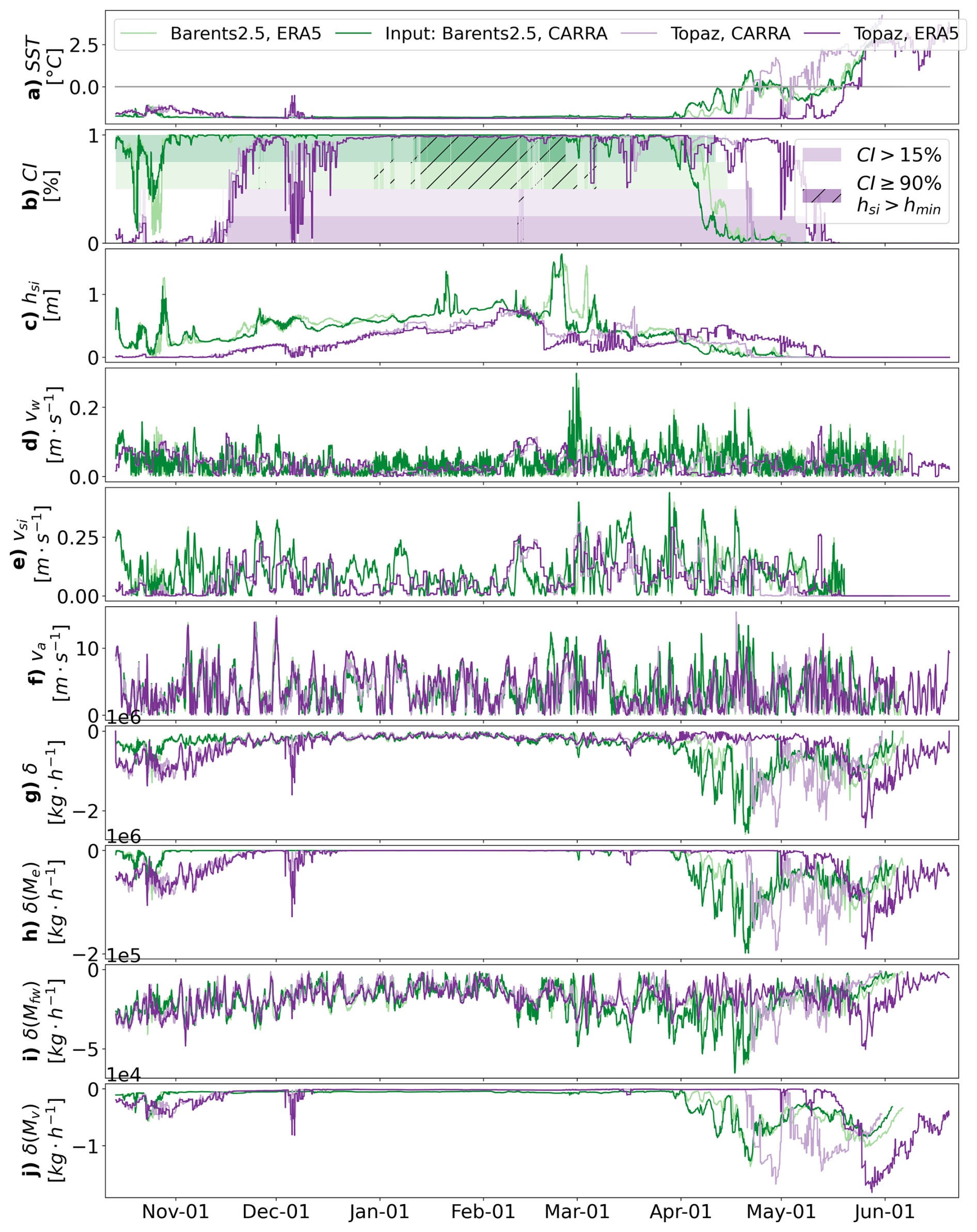
Figure 9 Time series of iceberg and environmental characteristics along the trajectory of iceberg 2013-788. Environmental input along the trajectory with (a) sea surface temperature SST [ °C], (b) sea ice concentration CI and time steps with CI >15 % (colour) and CI ≤90 % with h_si>h_min (colour, hatches), (c) sea ice thickness h_si [m], (d) surface water speed v_w [m s⁻¹], (e) sea ice drift speed v_si [m s⁻¹], (f) 10 m wind speed v_a [m s⁻¹]. Time series of iceberg deterioration during the drift with (g) iceberg mass loss per time step [kg 2 h⁻¹] and contribution δ [kg 2 h⁻¹] by (h) wave erosion M_e , (i) basal melt M_fw and (j) buoyant convection M_v.

Table 5 Statistics of environmental conditions along the of the trajectory of iceberg 2013-788 with relative number of days in conditions with CI >15 %, average sea ice concentration (CI), thickness (h_si), sea surface temperature (SST), and total speed of 10 m wind v_a, sea water surface v_w and sea ice v_si, along the trajectory. The sea ice speed is averaged over time periods with sea ice (CI >15 %).

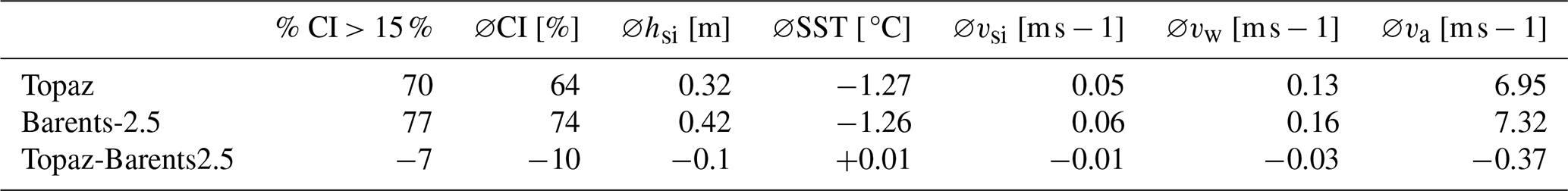
Table 6 Difference of mean total 2-hourly deterioration rate (δ, 10⁴ kg 2 h⁻¹) and relative contributions by the deterioration terms (δ(M), %) in the trajectories of iceberg 2013-788 with different environmental input. The deterioration terms are melt erosion M_e, basal melt M_fw and buoyant vertical convection M_v

5 Discussion

We investigate the impact of varied ocean, sea ice, and atmospheric input from four selected reanalyses, hindcasts and forecasts on the results of iceberg drift and deterioration simulations. We found that the environmental input causes a wide range of differences in the simulated iceberg characteristics.

5.1 Impact of environmental input on iceberg characteristics

5.1.1 Impact of ocean and sea ice variables on iceberg drift and deterioration

Ocean and sea ice variables have a large impact on the iceberg deterioration terms. Barents-2.5 yields larger values of CI (+4 %) and a longer exposure to sea ice in the iceberg pathways (+23 %). This reduces the deterioration due to wave erosion in the iceberg simulations (−19 %, Table 3). The impact of varied sea ice on iceberg deterioration is illustrated in the example of iceberg 2013-788 which shows smaller deterioration under Barents-2.5 input (Tables 5, 6) and rapidly increasing deterioration terms when the icebergs drift out of the sea ice edge in April and May 2014 (Fig. 9). This illustrates how the sensitivity of iceberg simulations to sea ice input is driven by the large impact on drift and deterioration, as well as the extensive occurrence of sea ice in the iceberg pathways. The average lower SST in Barents-2.5 (−0.41 °C) in the iceberg pathways due to coupling with excessive sea ice (Sect. 3) decreases the deterioration for all terms (Table 3). This finding agrees with the previously found anti-correlation between SST and iceberg age in Keghouche et al. (2010). Larger water velocities in Barents-2.5 (+0.05 m s⁻¹) may explain larger basal melt, despite larger average Topaz SST (Sect. 3 and Table 3), which is also illustrated in the example of iceberg 2013-788 (Table 6). As a result, the total deterioration is smaller in simulations with Barents-2.5 input and favours longer drift duration and drift distance along the trajectory. Our findings also agree with the previously described relative importance of the deterioration terms (El-Tahan et al., 1987; Eik, 2009a) and sensitivity to the variables contributing to the iceberg drift (Kubat et al., 2005; Eik, 2009b; Keghouche et al., 2009, 2010).

5.1.2 Impact of ocean and sea ice variables on iceberg extension

The differences in deterioration rates, drift duration and distance also cause variations in how far icebergs drift seasonally. Thus, varied ocean and sea ice input cause relatively large differences in the seasonal iceberg extension in autumn (August–September) and early winter (November–December) (Fig. 6). This is because the seasonal and interannual variability of iceberg extension is inherited from the temporal variability of environmental variables. Keghouche et al. (2010) discovered a correlation between iceberg extension, CI and SST and we find similar dynamic (CI) and thermodynamic (SST) effects on the iceberg extension. Sea ice reduces the deterioration rate of the icebergs and may decrease the iceberg drift speed. Higher temperatures and melt rates outside the sea ice limit the spread in the domain. We also find that sea ice increases the iceberg extension in spring, when icebergs drift far south within the sea ice, as the melt rates within the sea ice are low and sea ice expands far south. After the sea ice retreats in summer, icebergs are exposed to higher deterioration rates, limiting the spread in the domain until the sea ice expands again. Therefore, the onset of sea ice growth in autumn could be a deciding factor for the iceberg extension later in the year. This timing of freeze-up and melt differ in Topaz (too fast, see Xie et al., 2017a; Xie and Bertino, 2022) and Barents-2.5 (delayed compared to Topaz, see Sect. 3). Keghouche et al. (2010) found no correlation with sea ice thickness, however, we found that the exposure of iceberg to heavy sea ice and thus drift speed varies considerably between Topaz and Barents-2.5 (Fig. 2, Table 2). Seasonal differences in wind speed and direction might contribute as well.

The iceberg extension is also influenced by the exact seeding, with size, position and seeding date, which varies within defined parameters in the statistics of this study and varies in other studies. In this study, the seasonal cycle is steered by iceberg seeding between July and November, so that lowest iceberg extension occurs just before the start of seeding in July and the larger extent occurs just after the end of the seeding, in late November. Seasonal seeding likely causes the difference to the seasonal cycle of iceberg extension in Keghouche et al. (2010) with maximum extension in June–July and minimum in October to November. The impact of the seeding seasonality on the iceberg extension is larger than the impact of the environmental input.

5.1.3 Impact of ocean and sea ice variables on iceberg density

The differences in deterioration rates, drift duration and distance ultimately also cause large spatial differences in spatial iceberg density, for example, around Svalbard and Franz-Josef-Land in Fig. 5. Differences in iceberg density with varied input are as large as the absolute density and thus highly relevant. In general, iceberg density is largest in proximity to the iceberg sources (as in Keghouche et al., 2010), as the average effective drift distance is only around 100 km (Sect.4.1). The general distribution of the icebergs within the domain agrees with the findings of previous studies (e.g. Keghouche et al. (2010); Monteban et al. (2020)). The iceberg density is larger for simulations with Topaz input close to the coastlines and larger for simulations with Barents-2.5 input at slightly greater distance to the coastlines. This may be due to higher Barents-2.5 water speeds along the coastlines (Sect. 3) that transport the icebergs towards the open oceans more quickly. The simulation results along the coastlines need to be viewed in the light of large uncertainty of the environmental data in coastal regions.

Higher iceberg densities in simulations with Barents-2.5 input in the northernmost parts of the domain may be explained by Barents-2.5's average lower SST, higher concentration and more frequent (heavy) sea ice (Fig. 2), which increases the iceberg lifetime and traps the iceberg in those regions, as mentioned earlier by Keghouche et al. (2010).

Larger density to the north-west (north-east) of Bjørnøya under Topaz (Barents-2.5) input may result from large input differences in SST, water velocity and sea ice around the bathymetric feature of Storfjorden Trough, Spitsbergen Bank and Hopen Trench (Sect. 3). In contrast to Topaz, Barents-2.5 has complex spatial and temporal differences in water speed and direction, as it represents more local processes, including a strong tidal component and topographically-steered currents around Spitsbergen Bank. The more extensive sea ice cover over the Spitsbergen Bank in Barents-2.5, and the resulting reduced melt rate by wave erosion increases the number of icebergs drifting as far south as Hopen Trench.

5.1.4 Effect of tides on iceberg characteristics

The ocean input by Barents-2.5 further increases the drift duration, distance (Track) (Sect. 4.1), and local iceberg density (Sect. 4.2) by iceberg looping, as it prevents the icebergs from drifting directly into warmer waters, prolongs the track length and the time spent in a region. As a consequence, average domain and local peak iceberg densities are higher for simulations with Barents-2.5 input (Sect. 4.2). However, ocean input showed little impact on the effective drift distances. One might conclude that the tidal component is not essential to how far icebergs drift effectively in the Barents Sea (effective drift distance and extent, Figs. 3 and 4), however, we found that it is essential for simulating individual iceberg trajectories (Sect. 4.4), how long icebergs drift (drift duration, Fig. 3) and how many icebergs drift in different regions of the domain (regional iceberg density, Fig. 5).

Iceberg 2013-788 is influenced by tides, due to the oscillation of sea water speed along the trajectory (Fig. 9), but tidal forcing is too small in this example to be seen in Fig. 7. A relatively small influence by the tides may also explain characteristics of iceberg 2013-788 that contradict the above described statistics (longer drift duration and track for icebergs with Topaz input and longer effective distance for trajectories with Barents-2.5 input). Other iceberg trajectories in the simulations of this study showed examples with visible tidal looping, mostly in shallow regions where the tidal velocity is largest (e.g. Spitsbergen Bank).

5.1.5 Impact of atmospheric variables on iceberg characteristics

Wind input causes significant differences in iceberg density on small spatial scales. Higher horizontal resolution may cause higher wind speeds and (more accurate) atmospheric input between the islands of the Svalbard and Franz-Josef-Land archipelago, along their coastlines and in their fjords. The deviations of ERA5 and CARRA over sea ice (Sect. 3) are compensated by the low sensitivity of the iceberg drift to wind input (within sea ice). In some regions varied ocean, sea ice, and atmospheric input add up or cancel each other out, however the impact of varied ocean and sea ice input generally dominates. The iceberg density is not impacted by atmospheric input on large scales.

The example of iceberg 2013-788 illustrates the impact of environmental model physics, here wind representation over sea ice present in November 2013 to April 2014 (Fig. 9). The results are trajectories with small impact of wind input on large spatial scales, but visible impact on smaller spatial and temporal scales.

Wind input impacts seasonal iceberg extension on the same scale as varied ocean and sea ice input. Wind connected to large scale atmospheric patterns may also have an (delayed) impact on the interannual iceberg extension, as described in Keghouche et al. (2010).

Atmospheric input has no relevant impact on the drift distance (track, effective) or the spatial extent. The minor impact of atmospheric input may be explained by high similarity of ERA5 and CARRA wind over open ocean, due to the extensive use of ERA5 in CARRA (Hersbach et al., 2020; Køltzow et al., 2022, Sect. 3).

5.1.6 Diverging trajectories and impact of resolution

The example of iceberg 2013-788 demonstrates how identical initial conditions and small differences in the environmental input can result in diverging trajectories (causing increasing difference in input). This is due to the known tendency of Lagrangian trajectories to diverge and due to differences in environmental input, that induce differences in trajectory and further input differences. (Keghouche et al., 2009) described a rapid increase in the error in the iceberg simulation after two months.

The large impact by small environmental input differences can also be seen in the time period between 1 April and 15 May, when the iceberg 2013-788 drifts out of the sea ice and into regions with different ocean regimes (Figs. 9, 8). There, small change in iceberg position and different drift timing cause large difference in the exposure to environmental conditions and thereby iceberg drift and deterioration. This is also the case for coastal areas. It highlights the importance of temporal and horizontal resolution of the environmental data. An improvement in ocean and sea ice models would lead to extensive improvements in the iceberg simulations. In association, we observed that the high resolution of Barents-2.5 and CARRA allows icebergs to drift between islands and into fjords.

5.1.7 Impact of environmental input vs. regional and temporal variability

The difference in the simulation results (e.g. iceberg deterioration, drift duration, distance and seasonal iceberg extension, seen for the different iceberg sources in Fig. 3 and seasonal seeding in Fig. 6) due to varied environmental input are smaller than the spatial and temporal variability of the environmental variables in the domain. The spatial variability of iceberg characteristics with the environmental input differences (e.g. SST difference in Barents-2.5 and Topaz) are dominated by the spatial differences in environmental regimes (e.g. iceberg size and regional sea ice characteristics). For example, icebergs from Franz-Josef-Land are larger, more frequently locked in sea ice due to the more extensive sea ice around Franz-Josef-Land, causing larger drift durations and spread in the domain (see also Keghouche et al., 2010) compared to smaller icebergs from Novaya Zemlya that drift in mostly open waters. The temporal variability of iceberg characteristics (e.g. temporal iceberg extension) with the environmental input differences (e.g. in CI) is dominated by the seasonal and interannual variability of the environmental variables (e.g. the seasonal cycle of CI). This also means that the different environmental datasets distinguish the regionally and temporally varying environmental regimes well (in e.g. SST and CI). A similar representation of the environmental regimes may lead to similar main iceberg pathways.

5.1.8 Similarities in the iceberg characteristics despite varied environmental input

Despite the large impact of ocean and sea ice input on iceberg drift and deterioration, and local impact of wind input described above, we found similar main pathways, maximum spatial iceberg extent and southernmost latitude to where icebergs drifted (approximately 72° N). This may result from a similar general representation of the regional differences (e.g. between Central Bank and Spitsbergen Bank) in Topaz and Barents-2.5. One might conclude that the environmental input is not essential for simulating the main pathways and that these pathways are comparable in various studies.

5.2 Recommendations for practical applications

In the following, we discuss the suitability, advantages and disadvantages of the environmental model data (e.g. temporal availability and resolution of environmental data) as input in exemplary applications of iceberg simulations (e.g. long term statistics or short-time forecast of individual trajectories). This approach intends to support an informed decision on environmental input for iceberg simulations in future studies. We thereby outline which specific characteristics of an individual model (e.g. tides in Barents-2.5) causes which impact on iceberg simulations (e.g. spatial distribution). Note that we cannot provide generalised practical recommendations on which environmental data performs best as input to iceberg simulations, as the suitability is highly sensitive to the simulation goal, region, time period and model characteristics such as temporal and spatial availability, uncertainties, storage space and ease of access. The general lack of iceberg observations in the Barents Sea makes validating the statistics difficult.

5.2.1 Long-term statistic applications, input availability, and comparability of studies

Based on the above analysis, applications, including long-term statistics of iceberg pathways and the southernmost spatial iceberg extent (e.g. for analysing the long-term exposure of structures in the Central Barents Sea) are not sensitive to their environmental input. However, they are influenced by the availability of the input data (Bigg et al., 1997; Kubat et al., 2005; Eik, 2009b) and likely benefit from a wide time availability and consistency (e.g. in Topaz, ERA5 and CARRA). This study is strongly limited temporally and spatially due to the low availability of Barents-2.5.

The independence of the main iceberg pathways from the environmental input and the general similarity between the studies (e.g. in distribution of icebergs in the domain (Fig. 4) makes statistical iceberg studies comparable. Thus, the findings of this study are projectable on other studies, if accounting for the impact of different climatic conditions and different seeding conditions. We highlight that we do not study absolute iceberg characteristics as previous studies, but their differences due to varied environmental input. We highlight the novelty of this study, quantifying the impact of different types of common environmental models in iceberg simulations.

5.2.2 Application of regional iceberg density simulations

In applications simulating regional iceberg density (e.g. for planning of shipping routes around Spitsbergen Bank), the choice of input data is highly relevant. Differences in iceberg density are caused by different representation of ocean velocities, water temperature and sea ice, as e.g. found between Topaz and Barents-2.5 (Sect. 3) in the region around Bjørnøya. The region is characterised by warm Atlantic water inflow in the deeper parts (Storfjorden Trough and Hopen Trench), and southward cold-water transport in the shallower areas (Spitsbergen Bank), steering the water temperature and limiting the sea ice extent.

There, the topographically-steered currents and strong tidal influence in the shallow areas are described more extensively in Barents-2.5 (Fritzner et al., 2019; Röhrs et al., 2023; Idžanović et al., 2023, 2024). Topaz shows lower velocities, smaller gradients, and issues with simulating the circulation of Atlantic water inflow and the topographic steering (Sect. 3, Xie et al., 2017a). The sea surface velocity must be treated with special care, as the general lack of observations, limits the predictive skill of its forecasts and limits the constriction to observations in reanalyses. Despite the resulting low predictive skills in water velocities in both models, Barents-2.5 may still benefit from the representation of tides, the effect of air pressure on the water surface, and high spatial and temporal resolution, compared to Topaz (Röhrs et al., 2023b).

Sea ice and SST show large differences and uncertainties in Topaz and Barents-2.5 along the inflow of warm Atlantic waters and the spring sea ice edge (Sect. 3, Xie et al., 2017a; Xie and Bertino, 2022; Röhrs et al., 2023; Idžanović et al., 2024). Overall, the decreased deterioration and elongated drift with Barents-2.5 input may be unrealistic due to its excessive representation of sea ice and too small SST known in the community. Despite the large uncertainties, Topaz's SST and sea ice variables are closer to observations which may allow for more realistic iceberg deterioration and therefore potentially also more realistic extent and density. This applies especially for the years from 2010 to 2014, as the Barents-2.5 hindcast is a free-run, which tends to drift off, due to its missing constrain to input after the start of the model run (Idžanovic, pers. communications, 2024). Due to the large impact of sea ice representation on the iceberg simulations, it is therefore critical how well input data captures regional environmental regimes. Due to the large impact of sea ice concentration, iceberg simulations may benefit from using satellite-based CI products, although these are assimilated into the sea ice models already (e.g. Topaz, Barents-2.5 Forecast).

Due to the local impact of wind input on iceberg density, we recommend considering also the choice of atmospheric input.

5.2.3 Application of individual iceberg trajectories

In the application of simulating individual trajectories of icebergs (e.g. to estimate the potential exposure of structures and ships), the choice of input data is highly relevant as drift and deterioration is dependent on all environmental variables (including wind), their spatial and temporal resolution and the tidal representation. Due to its high horizontal and temporal resolution, the use of Barents-2.5 may be beneficial in iceberg simulations, compared to the lower resolution Topaz data. We also recommend simulating an iceberg ensemble to account for uncertainties in the environmental input and initial conditions.

6 Conclusions

In the absence of sufficient iceberg observations in the Barents Sea, numerical simulations of iceberg drift and deterioration serve as the most reliable source of data for iceberg statistics. We simulated a large number of iceberg trajectories with varying environmental conditions in the Barents Sea and the years 2010–2014 and 2020–2021. We quantitatively confirm and novelly describe how the results of such simulations are sensitive to the input from ocean, sea ice and atmosphere reanalyses or forecasts. To explain these results, we statistically compared the environmental models in light of existing model validations. The findings are intended to guide the selection of environmental input and the critical analysis of iceberg model simulations.

We found that the environmental input influences the iceberg simulations results depending on the simulation goals, temporal and spatial settings and the environmental model uncertainty and availability. The sea ice input is especially relevant for estimating the exposure of structures or (seasonal) ship routes in icy waters. Decreased iceberg deterioration, longer drift duration, and altered iceberg density are caused by an average −0.41 °C lower SST, 4 % higher sea ice concentration and 23 % more extensive sea ice occurrence in the iceberg pathways in Barents-2.5, compared to to Topaz. The representation of the onset of freeze- and melt-up in the sea ice models steers the annual and multi-annual spread of icebergs in the domain (iceberg extension). The simulations using Barents-2.5 may be unrealistic due to excessive sea ice in Barents-2.5 (especially in the Hindcast, 2010–2014) compared to input from Topaz that is closer to the observations, despite large uncertainties (e.g. in the marginal ice zone) and a delayed seasonal cycle. Decreased uncertainty in the ocean and sea ice model would lead to significant improvements in iceberg simulations. The iceberg drift and density are further enhanced by a 0.05 m s⁻¹ larger water speeds, tides and topographically-steered currents in Barents-2.5 (e.g. around Storfjorden Trough). This detailed local representation in Barents-2.5 is likely beneficial for iceberg simulations (e.g. for individual iceberg trajectories in shallow waters) despite its generally low skill in water velocity. Wind shows little impact on most iceberg characteristics, but the choice of higher-resolution input (e.g. CARRA) may be considered for simulations of local iceberg density and individual iceberg trajectories. In applications simulating individual iceberg trajectories, high temporal and horizontal resolution of the environmental data is important, as even small differences in the environmental input can result in diverging trajectories (e.g. as seen in the exemplary of iceberg 2013-788). We highlight the importance of the input resolution in coastal regions, despite its unreliability due to the lack of other (both environmental and iceberg) data. The difference in iceberg characteristics are dominated by the regional and seasonal regimes, which are represented in both Topaz and Barents-2.5. This may be the reason for similar iceberg pathways and their southernmost extent independent of the environmental input.

We highlight that the study is restricted to the years 2010–2014 and 2020–2021, the Barents Sea and the specific setup of the iceberg model, due to temporal and spatial availability of the input data and the study goals. We also emphasise that we cannot provide clear suggestions on the best choice of environmental data in iceberg simulations, due to the diverse characteristics of the input data and the multifaceted impact on the simulations. However, the findings widely agree with previous findings, are projectable on other settings and will facilitate the informed choice in environmental data. We note that the choice in ocean, sea ice and atmosphere models exhibits a focus on European and Norwegian models, which is motivated by the location of the study area in the European Arctic and the accessibility to research purposes. We highlight the opportunity to extend this study using a larger number of suitable ocean, sea ice and atmosphere models that are disregarded in this study. Future studies will also concern themselves with conducting similar studies for a larger number of years, different regions (e.g. west Greenland) and assessing the performance of the iceberg simulations (under varied input) by comparing to iceberg drift observations.