Saharan dust impacts on the surface mass balance of Argentière Glacier (French Alps)

Saharan dust deposits frequently turn alpine glaciers orange and darken their surface. Together with other light-absorbing particles, mineral dust reduces snow albedo, increases snow melt rate, and lowers the surface mass balance of glaciers. Since the surface mass balance drives the evolution of alpine glaciers, assessing the impact of impurities helps to understand their current and future evolution. The location of impurities within the snowpack and their effect on snow albedo can be estimated through physical modelling. In this study, we quantified the impact of dust, taking into account mineral dust and black carbon in snow, on the Argentière Glacier over the period 2019–2022. Our results show that during the three years preceding 2022, the contribution of mineral dust to the annual decrease in surface mass balance was between 0.31–0.45 m w.e., while it reached the double in 2022 with 0.63 m w.e. [0.54, 0.69] (median, [Q10–Q90]), and up to 1.2 m w.e. [0.9, 1.4] at specific locations. The impact of dust in snow was unevenly distributed over the glacier, especially in 2022. The highest simulated impacts occurred where firn layers from previous years were exposed after the total melt of the snowpack of the previous winter. The gravitational redistribution of the snow from avalanches was not taken into account, which can reduce the impact of dust at specific locations. Increasing the modelled scavenging efficiency of black carbon can double the impact of dust alone at the glacier scale. In general, the contribution of mineral dust to the melt represents between 8 % and 16 % of Argentière Glacier summer melt depending on the year. Hence, we recommend accounting for impurities to simulate the distributed surface mass balance of glaciers.

1 Introduction

In the European Alps, the surface mass balance (SMB) is a key component of the evolution of glaciers, as it controls the total mass budget of alpine glaciers (Cuffey and Paterson, 2010). When the surface of a glacier is at the melting point, a positive surface energy budget enables the glacier surface to melt. For alpine glaciers, the variability of this surface energy budget is mainly driven by shortwave radiation, e.g., Sicart et al. (2008). In mountainous areas, the incoming shortwave radiation strongly varies with the local topography (Arnold et al., 2006; Robledano et al., 2022). At the glacier surface, the shortwave radiation budget is modulated by the snow and ice albedo (Warren, 1982; Gardner and Sharp, 2010). The albedo of snow is determined, among other parameters, by snow properties and light-absorbing particles (LAPs) such as mineral dust (dust) or black carbon (BC). The evolution of LAP concentration at the glacier surface therefore modulates the glacier SMB.

The impact of LAPs is not restricted to the European Alps. By lowering the albedo, LAPs contribute to significantly accelerate snow and glacier melt around the world, e.g., Ménégoz et al. (2014), Ginot et al. (2014), Magalhães et al. (2019), Sarangi et al. (2020), Gilardoni et al. (2022), Gunnarsson et al. (2023), Menounos et al. (2025). In the Andes and High Mountain Asia, high LAP deposition fluxes and high melt impacts motivated these studies. In the European Alps, only a few studies quantified the impact of LAPs on glaciers, while the impact of LAPs on the melt of seasonal snow has been quantified by numerous studies, e.g., Di Mauro et al. (2019), Tuzet et al. (2020), Réveillet et al. (2022), Di Mauro et al. (2024). For instance, on average over the past 40 years, the presence of LAPs in snow has advanced the snow melt-out date by 18 d in the French Alps, and even more at high elevations (more than 20 d at 3000 m a.s.l., Réveillet et al., 2022).

The radiative impact of BC has often been in the spotlight, e.g., Bond et al. (2013). However, BC emissions and depositions on the snowpack have decreased from the end of the 20th century in the European Alps, e.g., Sun et al. (2020), Grange et al. (2020), Réveillet et al. (2022). Mineral dust also has a significant impact on snow melt (Skiles et al., 2018) and on glacier melt, e.g., Sarangi et al. (2020). Regarding mineral dust depositions, Europe is mainly influenced by Saharan dust transport, which is the main contributor that represents between 50 % and 70 % of the total annual dust depositions (Ginoux et al., 2001). Above 2000 m a.s.l. in the French Alps, the impact of dust alone has advanced the snow-melt out date by more than 10 d (Réveillet et al., 2022). Réveillet et al. (2022) showed that the impact of BC and dust increased with elevation, but this increase was more pronounced for dust. Moreover, Dumont et al. (2020) also showed that the radiative forcing of dust presented large topographic gradients. This increase in the impact of dust with elevation is due to several reasons. First, the late depositions of dust in the European Alps with intense deposition events occurring usually after March (e.g., Moulin et al., 1998; Collaud Coen et al., 2004) impact less the melt at low elevations that starts earlier. Second, for the highest elevations, the melting period is longer and occurs in spring and summer that are period associated with higher shortwave radiation than winter (Dumont et al., 2020). Thus the impact of dust on the overall glaciers mass balance should be accurately quantified.

Quantifying the specific contribution of LAPs to the SMB of an entire glacier could be achieved using physical modelling. Indeed, by representing different physical processes, physically based models can simulate snow and ice evolution. Some models directly account for the impacts of the LAPs, e.g., the snow model SURFEX/ISBA-Crocus (Vionnet et al., 2012; Tuzet et al., 2017) or the Community Land Model (Flanner et al., 2007). To our knowledge, only one study modelled and quantified the time evolution of the impact of dust on the SMB of a glacier in the European Alps (Gabbi et al., 2015). The authors modelled the SMB at two locations on the Clariden Glacier in Switzerland over a century. They quantified the long-term impact of dust and BC with the re-exposure of contaminated firn layers and showed that Saharan dust lowered the mean annual SMB by 0.03–0.06 m w.e. and black carbon by 0.2–0.3 m w.e. They found that annual melt rates were amplified by only 2 % due to the presence of mineral dust and by 10 % due to the presence of black carbon. However, this study did not assess the impact of dust on the SMB over an entire glacier area despite the small surface area of this glacier. In addition, Clariden Glacier is located in the northern part of the European Alps, which is less exposed than the southern part to Saharan dust deposition, e.g., Baladima (2021). Hence, we do not expect these results to be directly transferable to other alpine glaciers.

This study therefore focuses on the following research question: what is the impact of mineral dust on the SMB of an alpine glacier? To address this question, we selected the Argentière Glacier during the period 2019–2022. Being part of the French glacier observatory GLACIOCLIM, Argentière Glacier is closely monitored and studied (e.g., Vincent et al., 2009; Rabatel et al., 2018; Kneib et al., 2024b). The year 2022 was characterized by a strong precipitation deficit and heat waves in the French Alps (Mittelberger et al., 2024; Gascoin et al., 2024), leading to an exceptional mass loss of alpine glaciers in spring and summer (Six et al., 2023; Berthier et al., 2023; Cremona et al., 2023). In addition, a significant Saharan dust deposition event occurred on 16 March 2022 (Gascoin et al., 2024). These events were preceded by notable Saharan dust deposition events in February 2021 (Dumont et al., 2023).

In this context, we simulated the distributed SMB of Argentière Glacier using the snow model SURFEX/ISBA-Crocus (Vionnet et al., 2012; Lafaysse et al., 2017; Vernay et al., 2022), which includes the Two-streAm Radiative TransfEr in Snow (TARTES, Picard and Libois, 2024) with an explicit representation of LAPs in snow (Tuzet et al., 2017). This model had already been used to model alpine glacier SMB (e.g., Dumont et al., 2012; Réveillet et al., 2018). We performed an ensemble of simulations to account for meteorological forcing uncertainties. The resulting SMB were evaluated using point SMB measurements from in-situ surveys, glacier surface facies derived from Sentinel-2 images, and distributed SMB retrieved from satellite observation and modelling (Kneib et al., 2024b). We also performed control simulations by deactivating the effect of mineral dust on albedo to quantify the variation of the SMB that can be attributed to dust depositions in snow.

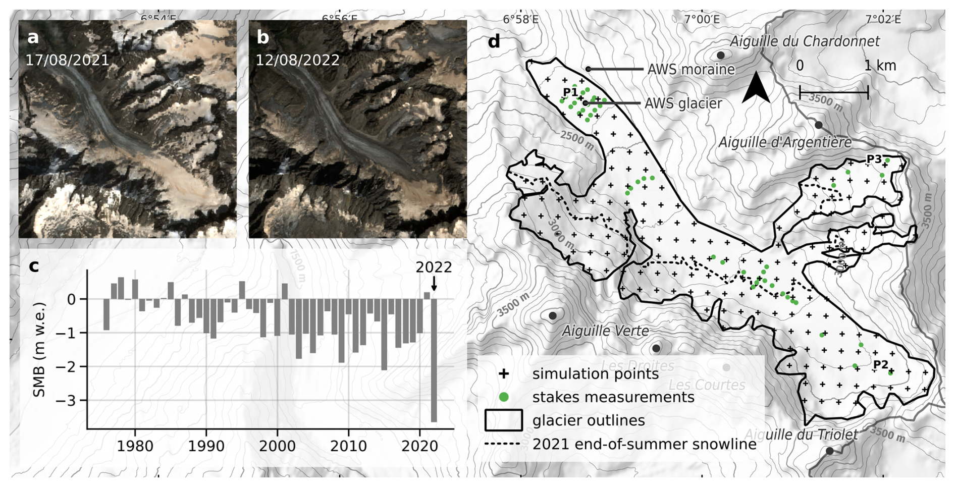
Figure 1 (a, b) True color Sentinel-2 images of Argentière Glacier on (a) 17 August 2021 and (b) 12 August 2022 (Sect. 2.2.2). (c) Annual glacier-wide surface mass balance of Argentière Glacier over the period 1976–2022 from the French glacier monitoring service GLACIOCLIM. (d) Map of Argentière Glacier. The 2021 end-of-summer snowline was manually derived from the 27 August 2021 Sentinel-2 image. Details of the SMB evolution at point P1, P2 and P3 are shown in Fig. 5. Background map from MapTiler.

2 Material and methods

2.1 Study site and topography

Argentière Glacier (45°57^′ N, 7°00^′ E) is located in the Mont-Blanc mountain range in France. The extent of the glacier is 11 km² in 2022, ranked 19th largest glacier in the European Alps, and the studied glacier area ranges from 3600 to 2100 m a.s.l. The main flowline of the glacier is 8 km long. This glacierized valley is mainly north-west facing (Fig. 1d) and surrounded by multiple peaks above 3800 m a.s.l. Argentière Glacier surface can be impacted by Saharan events, as shown in Fig. 1a which illustrates this phenomenon in August 2021, with an orange coloration observed in the glacier accumulation area. A dark orange color was visible in August 2022 (Fig. 1b), associated with an extreme negative mass balance in 2022 (Fig. 1c).

In this study, we used constant outlines of the glacier from the year 2019 (black line in Fig. 1d), and a digital elevation model (DEM) at a 10 m resolution from Copernicus. The DEM was used here for meteorological data downscaling, e.g., computation of direct solar radiation using a topographic mask (see Sect. 2.3.3). Simulation points (black crosses in Fig. 1d) were extracted from a two-dimensional grid at a horizontal resolution of 250 m using the Lambert 93 coordinate system (EPSG:2154).

2.2 Evaluation data

2.2.1 Point SMB measurements

Argentière Glacier is regularly monitored since 1975 by the GLACIOCLIM observatory (https://glacioclim.osug.fr/, last access: 23 September 2025). Winter accumulation measurements from autumn to spring and summer melt measurements from spring to autumn provide observed point winter and summer SMB along three ablation profiles of the main tongue (at 2400, 2500 and 2700 m a.s.l.) and in the two main accumulation areas (green points in Fig. 1d). Point SMB refers to the local surface mass balance, whereas glacier-wide SMB refers to the SMB integrated over the entire surface area of the glacier.

In this study, the annual SMB of year N refers to the hydrological year N, i.e., 1 October N−1 to 30 September N, and is expressed in metres of water equivalent (m w.e.). The accuracy of the point SMB measurements is estimated to be around 0.2 m w.e. (Thibert et al., 2008). Point winter SMB were used to adjust precipitation (Sect. 2.3.5). Point summer SMB measurements were used to evaluate the simulated summer SMB at the closest simulation grid point (Sect. 3.1).

2.2.2 Sentinel-2 optical satellite images

In this study, Sentinel-2 satellite (S2) images were used to (i) derive the surface type and mean snowline elevation to evaluate the simulations; and (ii) infer the glacier ice albedo. S2 images are optical, high-resolution and multispectral satellite images with a revisit time of at most 5 d. Here, we used bottom-of-atmosphere reflectances from Theia from the tile T32TLR containing Argentière Glacier (see Data availability). Those reflectances were corrected using the MAJA level-2A processor that performs topographic and atmospheric corrections (Hagolle et al., 2015). We used the reflectance of all spectral bands at 10 and 20 m spatial resolution. Bands at 10 m spatial resolution were resampled to 20 m with the cubic method. To avoid using images containing clouds, we visually selected a total of 21 cloud-free images acquired between May and October of the years 2019 to 2022 (detail on the date can be found in the Appendix Table B1). We selected only images between May and October because the glacier was often fully snow-covered outside of this period, which was not helpful for the evaluation.

2.2.3 Surface type derived from Sentinel-2 data

To evaluate our glacier simulations, we used a surface type classification derived from S2 images. The classification method splits the pixels into three different classes: ice, snow, and “not-glaciated”. The latter refers to pixels containing shadows, rocks, moraine debris, or liquid water. To develop the classification method, we manually labelled 8639 pixels using 216 polygons (5209 snow pixels, 1594 ice, and 1836 not-glaciated) extracted in the S2 images of Argentière Glacier. Appendix Fig. B1 shows the distribution of the pixels depending on variable R_B4, NDSI and RGND, where R_Bi is the S2 reflectance of band i, $\text{NDSI}=\frac{R_{\mathrm{B}\mathrm{3}}-R_{\mathrm{B}\mathrm{11}}}{R_{\mathrm{B}\mathrm{3}}+R_{\mathrm{B}\mathrm{11}}}$ and $\text{RGND}=\frac{R_{\mathrm{B}\mathrm{4}}-R_{\mathrm{B}\mathrm{3}}}{R_{\mathrm{B}\mathrm{4}}+R_{\mathrm{B}\mathrm{3}}}$. The central wavelengths of bands B3, B4 and B11 are respectively 560, 665 and 1610 nm. Based on the distribution of the labelled pixels and the optical properties of snow and ice (Warren, 1984; Dozier, 1989; Painter et al., 2013; Di Mauro et al., 2015; Gascoin et al., 2019; Flanner et al., 2021; Dumont et al., 2020; Di Mauro et al., 2024), the classification method was defined using three thresholds: a pixel was classified as “not-glaciated” if R_B4<0.12 or NDSI<0.5, and as snow or ice otherwise. In the last case, a pixel was classified as snow if $R_{\mathrm{B}\mathrm{4}}>-\mathrm{6.0}\times \text{RGND}+\mathrm{0.525}$ and as ice otherwise.

For each simulation point and S2 image, an S2 surface type was determined using the previous classification. The S2 surface type was snow (ice) if the snow (ice) pixels are in larger numbers in the 7×7 surrounding pixels around the simulation point, otherwise the S2 surface type was not defined. This S2 surface type was compared with the simulated surface type in Sect. 3.1 with the surface type error rate (frequency of error between the simulated and S2 surface types at all simulation points).

2.2.4 Sentinel-2 mean snowline elevation

For each selected satellite image, an S2 mean snowline elevation was computed (as illustrated in Appendix Fig. B2). For each image, we binned all classified pixel as ice or snow into 100 m elevation classes. Bin b_i refers to the bin between elevations E_i and E_i+100. Then, we defined b_j as the lowest elevation bins with more pixels classified as snow than ice. Hence, bin b_j−1 contains more pixels classified as ice than as snow. Finally, we computed the mean snowline elevation, between elevation E_j−50 and E_j+50, using a linear interpolation between the snow ratios in bins b_j−1 and b_j, as the elevation for which the snow ratio would be 50 %. This S2 snowline elevation was compared with the simulated snowline elevation in Sect. 3.1.

2.2.5 Sentinel-2 broadband ice albedo

The ice albedo was a parameter of our surface mass balance model. We inferred this parameter using S2 images and simulated ice spectra from the SNICAR radiative transfer model (Whicker et al., 2022). We computed eight spectral albedos of ice reflectance with different BC concentrations (75 to 1000 ng g⁻¹), at 10 nm resolution from 205 to 4995 nm with mid-latitude, clear-sky, summer irradiance conditions. These SNICAR spectra were used to interpolate between the S2 bands. For each S2 pixel classified as ice in the 21 selected images, we affected the SNICAR spectrum that minimized the RMSE between the SNICAR spectra and the S2 spectrum of the pixel. The spectral albedos from SNICAR were then weighted by the incident irradiance to obtain broadband albedos. We finally computed the ice albedo by averaging the SNICAR broadband albedo related to all the ice pixels. The resulting ice albedo on the 21 selected S2 images was 0.23 with a standard deviation of 0.05. This method is rather simple since we here aimed to quantify the impact of dust in snow, not in ice. Nevertheless, the sensitivity to this parameter was investigated in Sect. 3.3.

2.2.6 Broadband snow albedo derived from Sentinel-2 reflectances

Using all images of Table B2, we compared the modeled broadband albedo at noon, and the observed broadband albedo derived from Liang et al. (2003), i.e., $\text{S2 albedo}=\mathrm{0.356}\cdot R_{\mathrm{B}\mathrm{2}}+\mathrm{0.130}\cdot R_{\mathrm{B}\mathrm{4}}+\mathrm{0.373}\cdot R_{\mathrm{B}\mathrm{8}}+\mathrm{0.085}\cdot R_{\mathrm{B}\mathrm{11}}+\mathrm{0.072}\cdot R_{\mathrm{B}\mathrm{12}}-\mathrm{0.018}$ where R_Bi is the reflectance of Sentinel-2 band i. Appendix Fig. B3 shows this comparison. Only the points where the surface type (Sect. 2.2.3) was snow for both the model and S2 were used.

However, this comparison of absolute albedo has to be taken with cautious. Indeed, there are several limitations. First, the reflection of snow is not isotropic (e.g., Dumont et al., 2010), i.e., depends on the observation angle, and also varies with the solar zenith angle. Second, the uncertainties of the reflectance retrievals in complex terrain may be too high to estimate the accuracy of the simulated albedo, e.g., Cluzet et al. (2020). This is also highlighted on Appendix Fig. B3a where the computed S2 broadband albedo strongly depends on the slope.

2.2.7 Surface mass balance from Pléiades images

Following Kneib et al. (2024b), surface velocity and elevation change maps were extracted from Pléiades 4 m resolution DEMs and 0.5 m resolution ortho-images to estimate the distributed SMB of Argentière Glacier and its uncertainties at 20 m resolution for the period 8 September 2018 to 5 October 2022. Elevation change was obtained using six Pléiades DEMs from 8 September 2018, 25 August 2019, 17 September 2020, 30 September 2020, 15 August 2021 and 5 October 2022, and the ice flux was inverted from the 2012–2022 distributed surface velocity using three approaches and ice thickness scenarios to obtain the distributed SMB. In Kneib et al. (2024b), similar inversions for the period 2012–2021 were evaluated against the mean annual point SMB (described in Sect. 2.2.1). For the three inversion approaches, the RMSE was lower than 1 m w.e. yr⁻¹, showing good agreement between the resulting Pléiades annual SMB and point measurements.

Ultimately, in this study we used the mean of the resulting Pléiades SMB and the uncertainties of each of the three inversion approaches as our reference distributed SMB (Kneib et al., 2024b). We extracted the closest Pléiades SMB for each simulation point to evaluate the simulated SMB in Sect. 3.1.

2.3 Meteorological data

2.3.1 LAPs deposition fluxes

Mineral dust (dust) and black carbon (BC) hourly deposition fluxes were obtained from the CNRM-ALADIN63 regional climate model driven by the ERA5 reanalysis (Nabat et al., 2020). The prognostic aerosol scheme of ALADIN is called TACTIC (Tropospheric Aerosols for Climate In CNRM, coming from Morcrette et al., 2009, and used in Michou et al., 2015, 2020). The domain of the model included the Saharan desert with a southern limit roughly corresponding to +15° N, as shown in Fig. 1 of Nabat et al. (2020). The emissions of dust were computed by the model as a function of surface wind and soil characteristics (Nabat et al., 2020). Then, mineral dust was a prognostic variable of the model subject to atmospheric processes (transport and deposition). Anthropogenic and biomass burning emissions (including BC) were based on monthly inventories varying from year to year, namely the CEDS v2021-04-21 dataset for historical anthropogenic emissions (O'Rourke et al., 2021) up to 2019, extended up to 2022 following the study of Lamboll et al. (2021), and the GFED4.1s dataset (Randerson et al., 2017) for biomass burning emissions. The horizontal grid resolution of the CNRM-ALADIN63 outputs is 12.5 km. Only the nearest grid point output was used for all simulation points. This point was around 2 km from the glacier in a south-west direction. Over the complete simulation period, the mean dust and BC deposition fluxes of this nearest point were respectively 11.4 and 0.038 $\mathrm{g}{\mathrm{m}}^{-\mathrm{2}}{\mathrm{yr}}^{-\mathrm{1}}$. When considering the 3x3 CNRM-ALADIN63 grid points around this nearest point, the mean and standard deviation of the fluxes were 10.3 (±2.3) $\mathrm{g}{\mathrm{m}}^{-\mathrm{2}}{\mathrm{yr}}^{-\mathrm{1}}$ and 0.0433 (±0.011) $\mathrm{g}{\mathrm{m}}^{-\mathrm{2}}{\mathrm{yr}}^{-\mathrm{1}}$. ALADIN wet and dry depositions were redistributed with respect to the SAFRAN precipitation as in Réveillet et al. (2022), i.e., wet depositions when SAFRAN precipitations are positive, dry depositions otherwise.

LAPs deposition fluxes from ALADIN have been compared with in situ measurements in Tuzet et al. (2020) and their impacts on the snow melt-out date have been evaluated in Réveillet et al. (2022) using MODIS snow products. Moreover, Dumont et al. (2023) includes a dust mass measurement on Argentière Glacier during the extreme dust deposition event of February 2021. They measured 1.70 g m⁻² of mineral dust deposition at 2700 m a.s.l. on 8 February 2021 (measurement integrating the depositions from 5 February 2021 to 8 February 2021). On the other hand, the ALADIN model deposited in total 2.37 g m⁻² of dust from 5 February 2021 to 8 February 2021 at the nearest grid point from Argentière Glacier. Both values have the same order of magnitude, which is sufficient to assess the reliability of the model during this event given the difference in spatial resolution between the observation (sampling over an area of 105 cm²) and the simulation (with a spatial resolution of 12 km). The uncertainty related to the LAPs deposition fluxes is evaluated in Sect. 3.3 and discussed in Sect. 4.1.

2.3.2 Automatic weather stations

Two automatic weather stations (AWS) were located at the surface and on the right-hand side moraine with respect to the glacier flow of Argentière Glacier (Fig. 1d). The glacier AWS was located on the lowest part of the glacier (about 2400 m a.s.l.), during summer 2021 and recorded every 15 min from 20 May 2021 to 22 October 2021. The moraine AWS was maintained permanently and data was recorded continuously every 30 min from 1 January 2015 to 30 September 2022. The elevation difference between the two AWS is around 70 m, and they are located around 500 m apart (detailed location in Fig. 1d). Among other parameters, both AWS measured incoming shortwave radiation SW (W m⁻²), incoming longwave radiation LW (W m⁻²), air temperature at 2 m (K or °C) and wind speed (m s⁻¹). All measurement time series were averaged to a time-step of 1 h, that is the time-step of the SAFRAN data (Sect. 2.3.3). The measurement devices and the associated measurement uncertainties from the manufacturers were listed in Appendix Table C1. A comparison of the measured air temperatures is presented in Appendix Fig. C1 when both stations recorded. This comparison is used in Sect. 2.3.4.

2.3.3 SAFRAN data

The SAFRAN atmospheric reanalysis (Vernay et al., 2022) combines meteorological information at the mountain massif scale (here typically 1000 km² for the Mont-Blanc massif) from numerical weather prediction (ERA-40 reanalysis from 1958 to 2002, ARPEGE from 2002 to 2021) and in situ meteorological surface observations (2 m air temperature and humidity, 10 m wind, 24 h cumulative precipitations). SAFRAN provides hourly meteorological data (2 m air temperature and specific humidity, wind speed and direction, rainfall and snowfall rate, longwave incoming radiation, shortwave direct and diffuse radiations) with a 300 m vertical resolution. Those data were extracted from 1 August 2008 to 30 September 2022 and interpolated at each simulation point using their exact elevation following Revuelto et al. (2018). Moreover, direct shortwave radiation was masked using an illumination mask at 5° resolution computed for each simulation point. Examples of illumination masks and spatialized mean shortwave radiations are presented in Appendix Fig. C3.

Four SAFRAN variables (air temperature, wind, longwave and shortwave radiations) were bias-corrected based on the observed variables at the moraine AWS. For each variable V(t), for each season s from summer 2015 (winter from October to April, summer from May to September), we computed the bias $b^{\mathrm{s}}={\mathit{\mu }}_{V_{\text{saf}}}-{\mathit{\mu }}_{V_{\text{obs}}}$ for additive variables and $b^{\mathrm{s}}={\mathit{\mu }}_{V_{\text{saf}}}/{\mathit{\mu }}_{V_{\text{obs}}}$ for multiplicative variables, between the mean of the SAFRAN massif-scale analysis ${\mathit{\mu }}_{V_{\text{saf}}}$ and the mean of the moraine AWS observation ${\mathit{\mu }}_{V_{\text{obs}}}$ (numeric values in Appendix Fig. C2). This enabled seasonally bias-correcting of the SAFRAN variables at each time-step t following $V_{\text{saf, bias-corr.}}^{\mathrm{s}}\left(t\right)=V_{\text{saf}}^{\mathrm{s}}\left(t\right)-b^{\mathrm{s}}$ if the variable is additive (air temperature, longwave) and $V_{\text{saf, bias-corr.}}^{\mathrm{s}}\left(t\right)=V_{\text{saf}}^{\mathrm{s}}\left(t\right)/b^{\mathrm{s}}$ if the variable is multiplicative (wind, shortwave). This correction was propagated to all simulation points. It ensured that: (i) on a seasonal scale, the meteorological conditions extracted on the full massif scale did indeed reflect the conditions in the vicinity of the glacier; (ii) the SAFRAN variables and the observed variables were bias-corrected, which was an hypothesis needed to later apply stochastic perturbations (Sect. 2.3.6). Two more adjustments were applied to the SAFRAN data in Sect. 2.3.4 and 2.3.5.

2.3.4 SAFRAN temperature adjustment

The SAFRAN reanalysis assimilates exclusively observations outside of glacierized areas, so we adjusted the SAFRAN air temperature T which is an ambient, i.e., off-glacier air temperature. A difference was observed between both AWS in the case of a high air temperature (above 3.5 °C, Appendix Fig. C1). More precisely, the temperatures measured at the glacier AWS were lower than those at the moraine AWS. This difference for high temperature could be due to cooling from the ice surface or to katabatic down-glacier winds (Sicart et al., 2008; Shea, 2010; Shaw et al., 2023, 2024). A similar pattern was shown by Shaw et al. (2023) in their supplementary Fig. S5. In our case, the temperature sensitivity above 3.5 °C was TS=0.76 (K K⁻¹), which means that for every increase in 1 °C above 3.5 °C for temperatures outside the glacier, the temperature on the glacier only increased by 0.76 °C. Therefore, we adjusted the SAFRAN temperature T^∗, above T₀ = 3.5 °C without any upper bound, according to

$$\begin{array}{}\text{(1)}& T^{\ast }=\left\{\begin{array}{ll}\text{TS}\cdot (T-T_{\mathrm{0}})+T_{\mathrm{0}}& \text{if }T>T_{\mathrm{0}}\\ T& \text{otherwise}\end{array}\right.\end{array}$$

2.3.5 SAFRAN solid precipitation adjustment

Using SAFRAN precipitation data systematically underestimated the winter SMB of French alpine glaciers at high elevations (Gerbaux et al., 2005; Dumont et al., 2012; Réveillet et al., 2018; Vionnet et al., 2019; Gilbert et al., 2023). To address this issue, previous studies applied a correction factor to align the total winter precipitation with the observed winter SMB. This correction also accounted for the wind-blown snow redistribution. However, this approach did not account for winter melting events, which have become more frequent in recent years (e.g., a winter SMB of −1.44 m w.e. was measured punctually at the bottom of the main tongue at 2400 m a.s.l. of Argentière Glacier in 2022) and is therefore no longer suitable.

Thus, in this study, for a given winter, at a given point with an observed winter SMB, we associated the closest simulation point and its simulated winter SMB b_mod (m w.e.) with the initial solid precipitations sp. The targeted simulated winter SMB $b_{\mathrm{mod}}^{*}$ (m w.e.) with corrected solid precipitations should be equal to the winter SMB measurement b_mes (m w.e.), hence

$$\begin{array}{}\text{(2)}& b_{\mathrm{mes}}=b_{\mathrm{mod}}^{*}=K\times \text{sp}-M_{\text{winter}}=K\times \text{sp}-(\text{sp}-b_{\mathrm{mod}})\end{array}$$

where K is the multiplicative factor of this study at a given point and for a given winter, “sp” (m w.e.) the sum of the initial winter solid precipitation, $M_{\text{winter}}=\text{sp}-b_{\mathrm{mod}}$ the simulated melt during the winter (m w.e.). Here, we hypothesized that the simulated melt M_winter corresponded to the measured melt. Isolating K in Eq. (2) gave

$$\begin{array}{}\text{(3)}& K=\mathrm{1}+{\displaystyle \frac{b_{\mathrm{mes}}-b_{\mathrm{mod}}}{\text{sp}}}\end{array}$$

Using Eq. (3), we calculated the factors K for the winters 2018–2019 to 2021–2022 for all available point winter SMB (Appendix Fig. C2). Because more measurements were made on the lowest part of the glacier, and to avoid an overestimated impact of these on the upper part, we averaged all the K factors (all winters, all points) over 100 m bins. To obtain the final factors used in this study, we interpolated the aggregated factors K with a polynomial fit of the order one depending on elevation.

The final resulting factors ranged from 1.25 to 1.75 and increased with elevation. The explicit equation was $K=\mathrm{2.03}\times {\mathrm{10}}^{-\mathrm{4}}\cdot (E-\mathrm{2000})+\mathrm{1.38}$ (black dashed line in Appendix Fig. C2), where E is the elevation (m a.s.l.).

2.3.6 Meteorological forcing ensemble

Applying the adjustments in temperature (Sect. 2.3.4) and in solid precipitation (Sect. 2.3.5) to the SAFRAN data led to the adjusted forcing. From this, we built an ensemble of forcings with 40 members (Cluzet et al., 2020). This ensemble of forcings allowed us to take into account the meteorological uncertainties which generally prevail on the snow model uncertainties in the case of snowpack simulations (Raleigh et al., 2015; Günther et al., 2019). This also enabled us to estimate the meteorological uncertainties on the simulation results.

Five meteorological variables were perturbed (air temperature T, incoming direct shortwave radiation SW_dir, incoming longwave radiation LW, wind speed W and solid precipitations SP) using a first-order autoregressive model AR(1). The stochastic perturbation method was inspired from Charrois et al. (2016), Cluzet et al. (2020), and detailed in Appendix C1. For a given member, the same perturbations were spatially applied to all simulation points. Each variable was perturbed independently from other variables. For each variable, the perturbation term X_t depends on a decorrelation time τ and an amplitude ${\mathit{\sigma }}_X^{\mathrm{2}}$. The exact relationship is explained in detail in Appendix C1. Given an additive variable V_t (T or LW) at time-step t, the perturbed variable $V_t^{*}$ is defined as $V_t^{*}=V_t+X_t$, and in case the variable is multiplicative (SW or W), $V_t^{*}$ is defined as $V_t^{*}=V_t\cdot (\mathrm{1}+X_t)$. We applied the perturbations on a daily scale with a decorrelation time τ=24 h for T, SW_dir, LW and W, and on a season scale with ${\mathit{\tau }}_{\mathrm{SP}}=\mathrm{1500}\mathrm{h}=\mathrm{62.5}$ d for solid precipitations. For each variable, the amplitude ${\mathit{\sigma }}_X^{\mathrm{2}}$ of the meteorological uncertainties were induced by the standard deviation of the difference between the observed variable (at moraine AWS, Sect. 2.3.2) and the SAFRAN variable (interpolated at the location of the moraine AWS) over the period 1 January 2015–30 September 2022. For each variable, this standard deviation was σ_X=1.43 °C for T, σ_X=28.0 W m⁻² for LW, σ_X=142 W m⁻² for SW, σ_X=2.08 m s⁻¹ for W. For solid precipitations, we used the standard deviation between the modelled winter SMB (with the correction of solid precipitations of Sect. 2.3.5) and the observed winter SMB, for all measurements between 2300 and 2400 m a.s.l. over the period 2018–2022. This led to σ_X=0.36 m w.e.

2.4 Surface mass balance model

For each simulation point and associated forcing inputs described in Sect. 2.3, we performed independent simulations of SMB at 250 m horizontal resolution (Fig. 1d). The 250 m horizontal resolution was chosen as a trade-off between simulation costs and model performances, which generally drops at 500 m resolution in mountainous area, e.g., Baba et al. (2019). We used the detailed snowpack model SURFEX/ISBA-Crocus (Vionnet et al., 2012), which was already used to simulate glacier SMB regardless of the glacier size, e.g., Gerbaux et al. (2005), Lejeune et al. (2007), Dumont et al. (2012), Réveillet et al. (2018). Crocus simulates the evolution of the snow cover with a 15 min time-step representing different processes including thermal diffusion, phase change, water flow, snow metamorphism and compaction. Snow optical properties (single scattering albedo and absorption cross section for each snow layer) are calculated from the prognostic variables of the model (grain size, density, layer thickness). In Crocus, the snowpack is discretized as a one dimensional column with up to 50 layers, each of them having its own snow/ice properties. This layering is determined by an ensemble of rules described in Vionnet et al. (2012). An initial state of the glacier was prescribed at each simulation point, with a vertical column of several ice layers with a density of 917 kg m⁻³ as in Vionnet et al. (2019). The resulting height of the total column was initially set to an arbitrary value of 100 m w.e., with a temperature of 0 °C. The roughness length of snow z₀ was set to 0.5 mm, and the roughness length of ice was set to 2×z₀. These values were selected to obtain turbulent fluxes consistent with the measurements at the glacier AWS. This ratio between snow and ice roughness length was kept constant for the entire study. These values of roughness length were inside the usual ranges described in Cuffey and Paterson (2010). Ice albedo of 0.23 was inferred from S2 images (Sect. 2.2.5). Given the substantial influence of parametrization choices for albedo and roughness values on SMB (e.g., Réveillet et al., 2018), the sensitivity to these parameters was analyzed in Sect. 3.3.

We collected Crocus outputs every 6 h for all simulation points (total snow water equivalent (m w.e.), and broadband albedo). We also computed the mean density (kg m⁻³) in the top 5 cm of the simulation, named in this study top density. This fixed height allows us to be independent of the numerical discretization. We also derived the simulated surface type from the top density: ice if top density is higher than 850 kg m⁻³ (Cuffey and Paterson, 2010), else snow. The mean simulated snowline elevation was computed at simulation horizontal resolution (i.e., 250 m) using the same method as for the S2 images (Sect. 2.2.2) and was therefore compared to the mean observed snowline elevation from S2 images in Sect. 3.1. This allows us to evaluate the snowpack melt-out date.

2.4.1 LAP implementation

Since Tuzet et al. (2017), a parametrization allows Crocus to explicitly model the interactions between LAPs and snow. This parametrization was used in this study. Each snow layer contains a mass of each type of LAPs which enables to compute the spectral albedo of the snow surface at 20 nm resolution accounting for LAPs using the model Two-streAm Radiative TransfEr in Snow (TARTES, Picard and Libois, 2024). To this end, TARTES computes the light penetration and energy absorption using snow properties and the LAPs mass in each layer. In this study, we used two types of LAPs, mineral dust and BC. To compute the albedo of snow, the refractive indices of ice was set as in Réveillet et al. (2022). Particularly, the mass absorption efficiency of dust MAE_dust(λ) used for this study was the MAE of the Lybian dust from Caponi et al. (2017), i.e., ${\text{MAE}}_{\text{dust}}\left(\mathit{\lambda }\right)={\text{MAE}}_{\text{dust}}\left({\mathit{\lambda }}_{\mathrm{0}}\right)\times (\frac{\mathit{\lambda }}{{\mathit{\lambda }}_{\mathrm{0}}}{)}^{-{\text{AAE}}_{\text{dust}}}$ where λ₀=400 nm, ${\text{MAE}}_{\text{dust}}\left({\mathit{\lambda }}_{\mathrm{0}}\right)=\mathrm{71}\times {\mathrm{10}}^{-\mathrm{3}}$ m² g⁻¹, and the Ångström absorption exponent AAE_dust=3.2. The MAE of BC at 550 nm used for this study was 7.5 m² g⁻¹ (Bond and Bergstrom, 2006). To quantify the impact of dust, BC needed to be taken into account since the impact of dust relies on BC concentration in the snowpack. This is discussed in Sect. 4.2. For the two uncertainty tests on the dust MAE (Fig. 8), we used the highest and the lowest values of dust MAE considering the regions of Sahel and Sahara of Caponi et al. (2017), respectively [${\text{MAE}}_{\text{dust}}\left({\mathit{\lambda }}_{\mathrm{0}}\right)=\mathrm{27}\times {\mathrm{10}}^{-\mathrm{3}}$ m² g⁻¹, AAE_dust=3.3] and [${\text{MAE}}_{\text{dust}}\left({\mathit{\lambda }}_{\mathrm{0}}\right)=\mathrm{630}\times {\mathrm{10}}^{-\mathrm{3}}$ m² g⁻¹, AAE_dust=3.4].

The implementation of Tuzet et al. (2017) allows impurities to percolate with liquid water from one layer to the underlying one and prevent the complete accumulation of LAPs at the very top of the snowpack during melt. In Crocus, this process is parameterized for each LAP type with a scavenging efficiency. For large LAPs such as mineral dust, with a typical radius of 5 microns, Conway et al. (1996) explained that these particles stay near the snow surface, almost not percolating with liquid water, hence we set dust scavenging coefficient k_dust=0. For BC, the reference scavenging efficiency k_BC used by previous studies is 0.2 (e.g., Flanner et al., 2007; Gabbi et al., 2015), then we also chose this value as reference. Sensitivities to both scavenging efficiencies were presented in Sect. 3.3 and discussed in Sect. 4.2.

2.4.2 Model modifications

Since the Crocus model was primarily developed for avalanche forecasting, the layering rules discourage the merging of layers with different snow grain properties, e.g., most of the time a faceted crystal layer would not be merged with a rounded-grains layer, and a snow layer would not be merged with an ice layer. However, those initial layering rules allowed the merging of layer containing very different LAPs concentration if their microstructure properties were sufficiently close. When it occurred several times, especially with thick layers, this numerical process could artificially redistribute impurities across the entire snowpack. This spurious redistribution of LAPs, which modified their reappearance date during the melt period and their impact on albedo had to be avoided. Hence, we added a new merging discretization rule that prioritized the conservation of layers with high dust concentration. We chose to prioritize mineral dust because its concentration in seasonal snow is vertically more discontinuous than that of BC. However, layers containing a high concentration of both mineral dust and BC, e.g., top of the firn from the previous year, were preserved through the prioritization of layers with a high concentration of dust.

Two other modifications were implemented in the model. First, as the concentrations of mineral dust and BC in the ice were unknown, the TARTES radiative scheme was not used in case ice was at the top of the snowpack. The model considered ice at the top of the snowpack if the top density was higher than 850 kg m⁻³ which is close to the pore close-off density, and in this case, the albedo was set to a constant value inferred from Sect. 2.2.5. Hence, we did not model the difference in ice albedo between simulations with and without impurities. Second, we implemented an option to disable the effect of one LAP type on the spectral snow albedo. More precisely, the discretization rules stayed the same as in the reference version but the LAP acted as transparent in the radiative transfer model TARTES. This feature was used to quantify the impact of mineral dust and BC in Sect. 3.2.

2.5 Description of the simulation setup and metrics

All simulations included two phases: (i) the spin-up (2008–2018); (ii) the period of interest (2019–2022). The chronology and the use of the different data are summarized in Appendix Fig. A1. Initially, a column of temperate ice was prescribed for all simulations (Sect. 2.4), and the spin-up aimed to initialize the LAPs contents in old firn in the accumulation area and to reach a thermal equilibrium of deep ice layers.

The forcing ensemble was used as input to the simulation model to get the simulations considering the impact of mineral dust (simulations named “dust”), and the simulations without the impact of mineral dust (simulations named “no-dust”). Simulations without the impact of dust were obtained without the radiative effect of dust as explained in Sect. 2.4.2. As a result, we obtained 40 paired simulations (dust and no-dust). An important point is that BC remained present in all simulations. An alternative could have been to use the difference between (i) the simulation with dust and without BC, and (ii) the simulation without LAP at all as in Réveillet et al. (2022). This would have likely lead to larger quantified impacts (Flanner et al., 2012). However, we chose the simulation with both BC and dust as the reference as it is closer to the observed state of the snowpack, hence avoiding an overestimation of the dust impact and staying in line with other studies, e.g., Flanner et al. (2007, 2012). A fictive example of evolution of the glacier state with a single pair of the ensemble is presented in Fig. 2. This illustration reminds that the impact of dust was only taken into account in snow and firn, not in ice. However, in the ablation area, by advancing the snow melt-out date, simulations with LAPs expose the ice earlier than simulations without LAPs. Since the albedo of ice is lower than the albedo of snow, ice acts as a positive feedback for melt and leads to a lower summer surface mass balance. To quantify this feedback, we had to simulate both snow and ice. In the same way, Réveillet et al. (2018) showed that lower winter snow accumulation led to higher summer melt due to this feedback.

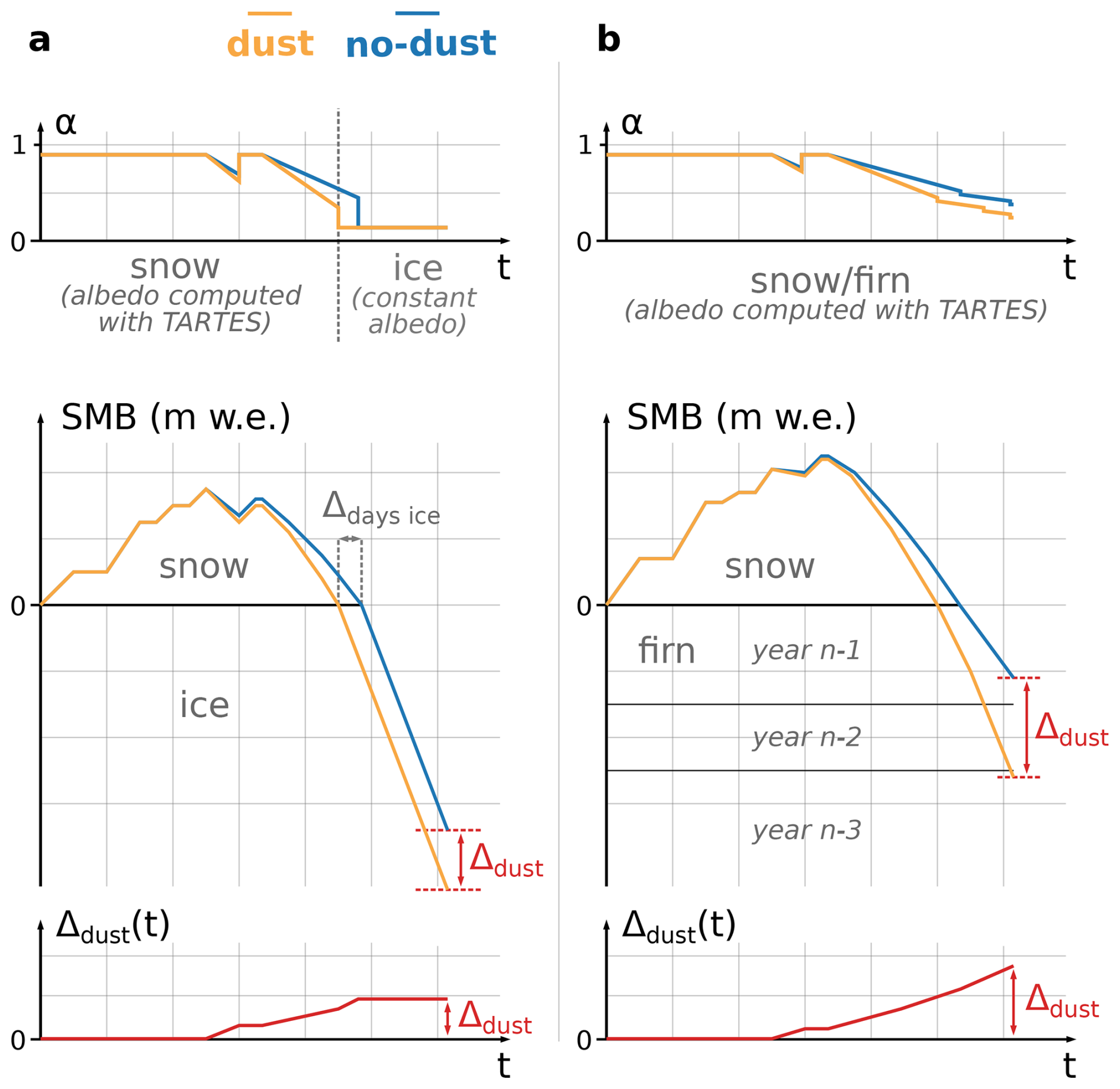
Figure 2 Possible evolution of the albedo, SMB and dust impact Δ_dust, over one year, with and without dust, for (a) a location in the ablation area where snow accumulated on ice during winter, and (b) a location in the accumulation area where snow accumulated on top of the firn from previous years.

We evaluated the SMB of the period of interest in Sect. 3.1. We analyzed the results during this period by comparing the years 2019–2021 to the year 2022 at each simulation point and at the glacier-scale (Sect. 3.2). To do so, we used the following metrics. The dust impact Δ_dust (m w.e.) was computed as the difference in annual SMB between dust and no-dust simulations. The melt fraction due to dust ${\mathrm{\Delta }}_{\text{dust}}/\text{M}$ (m w.e. $/$ m w.e.) was computed as the ratio between the dust impact Δ_dust and the total melt of snow and ice of the year in the simulation taking dust into account. The number of days with ice at the top of the simulation was called N_ice-days. The time duration during which ice was exposed in the simulation with dust and not exposed in the simulation without dust was computed as ${\mathrm{\Delta }}_{\text{ice-days}}={\mathrm{N}}_{\text{ice-days}}^{\text{dust}}-{\mathrm{N}}_{\text{ice-days}}^{\text{no-dust}}$. To find results at the glacier scale, we first averaged the values of all simulation points, and we then computed the median and Q10–Q90 of these averages at the glacier scale.

Outside of the ensemble framework, we also ran different simulations using the adjusted forcing and the reference model parametrization in which we modified either an input or a model parameter. This led to the sensitivity analysis of Sect. 3.3.

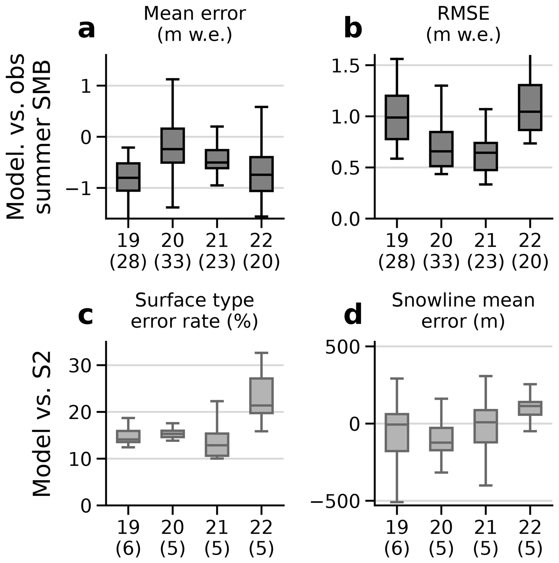
Figure 3 (a) Mean error between point measurements and modelled summer SMB for the summers 2019 to 2022 for the 40 members of the ensemble using q point measurements (in parenthesis). (b) Same as panel (a) with root mean square error. (c) Surface type error rate between Sentinel-2 and simulated surface type using p S2 images (in parenthesis) for the years 2019 to 2022. (d) Snowline mean elevation error between S2 and simulated snowlines using p S2 images for the years 2019 to 2022. All boxes in the figure show the quartiles of the distributions. The upper bound for the upper whiskers extends to a last value less than $\text{Q3}+\mathrm{1.5}\times (\text{Q3}-\text{Q1})$, and the lower bound for the lower whiskers extends to a first value greater than $\text{Q1}-\mathrm{1.5}\times (\text{Q3}-\text{Q1})$.

3 Results

3.1 Evaluation of the simulated SMB

Figure 3 illustrates the evaluation of the simulated annual SMB for the hydrological years 2019 to 2022. For each year, we computed the mean error and the root mean square error (RMSE) for all the simulated summer SMB against the point measurement of summer SMB (Fig. 3a, b), supported by 28, 33, 23 and 20 stake measurements, respectively. The spread of the ensemble included the zero mean error for the year 2020, 2021 and 2022. For all years, the summer simulated SMB were lower than the observations. Moreover, for each year, some members had a RMSE lower than 1 m w.e. against the summer point measurements. If we only consider the observed summer SMB under and above 2800 m a.s.l. (respectively 84 and 20 measurements), some members still had a RMSE lower than 1 m w.e. These errors can be compared to the total melt of snow and ice during the summer period, that is typically 5–9 m w.e. in the ablation area, 2–4 m w.e. near the snowline elevation, and 0–2 m w.e. in the accumulation area.

Then, we compared our simulations against S2 images. For the years 2019 to 2022, all members exhibit a surface type error rate between 8 % and 35 % computed over more than five S2 images per year. In addition, for each year, the zero mean snowline error was always within the spread of the ensemble. The evaluation of the no-dust simulations are presented using the observed summer measurements and the S2 images in Appendix Fig. D1.

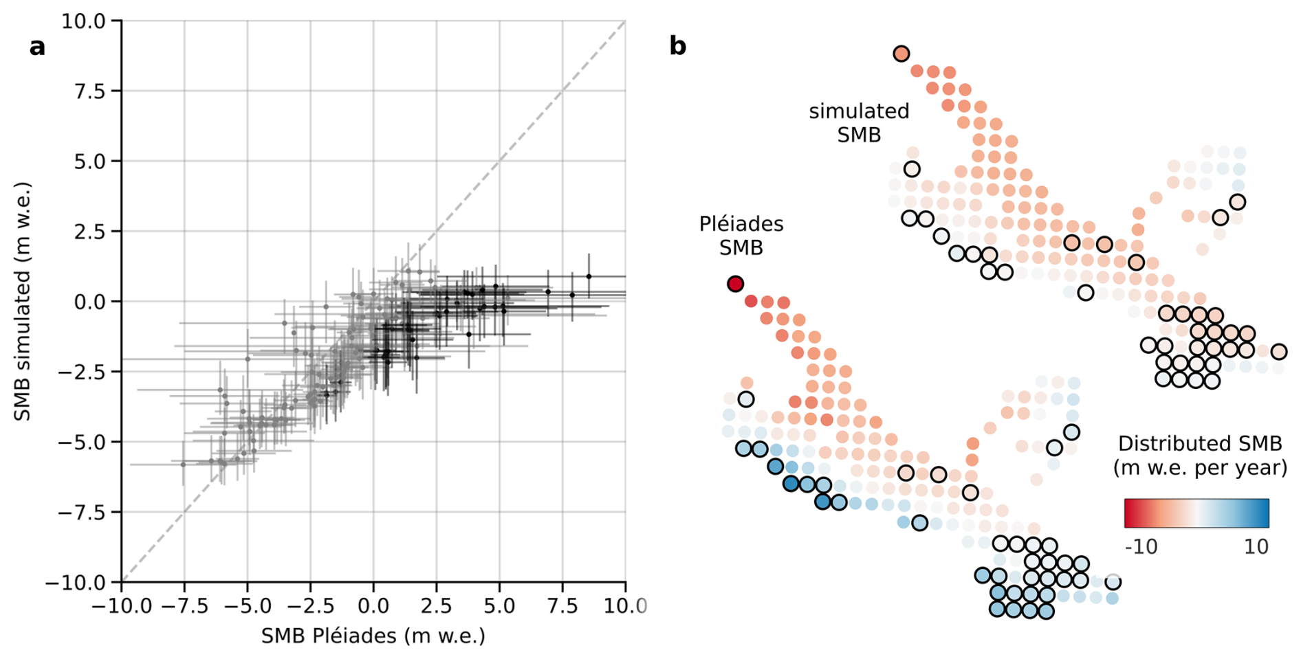
Figure 4 (a) Scatter plot of mean annual SMB inverted from Pléiades data vs. simulated SMB, over the period 8 September 2018 to 5 October 2022. Median-Q10–Q90 are represented for simulations, mean and a 2-standard deviations from the mean are represented for the Pléiades SMB. Points with uncertainty that do not cross the 1:1 line are plotted in black, the others in gray. (b) Distributed Pléiades and simulated SMB (medians). Points plotted in black in panel (a) are encircled in black.

Last, we compared the mean annual simulated SMB from 8 September 2018 to 5 October 2022 with distributed annual SMB derived from Pléiades elevation change and velocity fields, called here Pléiades SMB. Figure 4 shows that the distributed Pléiades SMB had higher extreme values (−15.2 to 8.6 m w.e. yr⁻¹) than the simulated SMB (−5.8 to 1.1 m w.e. yr⁻¹) and a higher variance with standard deviation of distributed SMB σ_Pléiades = 3.3 m w.e. yr⁻¹ and σ_simu = 1.8 m w.e. yr⁻¹. The glacier-wide Pléiades SMB was −0.7 m w.e. yr⁻¹, and the simulated SMB was −1.9 m w.e. yr⁻¹. For most of the simulation points (129, black points in Fig. 4), the Pléiades and simulated SMB uncertainties intersected. For a minority of points (31, red points in Fig. 4), Pleiades SMB uncertainties did not match the simulated SMB uncertainties. Most of those points were located on the southern part of the glacier, in the accumulation area, at the base of steep north-facing headwalls, where several Pléiades SMB points were higher than 3 m w.e. yr⁻¹ while the simulated SMB did not exceed 2 m w.e. yr⁻¹. This difference is likely due to avalanches and discussed in Sect. 4.3.

3.2 Simulated impact of dust

3.2.1 At the local scale in different sectors of the glacier

Figure 5 shows the evolution of the snow water equivalent relative to the 1 October for four hydrological years, from 2019 to 2022, at three different locations using the ensemble of simulations. Point P1 is in the ablation area, at around 2400 m a.s.l. Point P2 is in the accumulation area, above the end-of-summer snowline of 2021 but under the end-of-summer snowline of 2022, at around 2900 m a.s.l. Point P3 is in the accumulation area at around 3500 m a.s.l. (see exact locations in Fig. 1d).

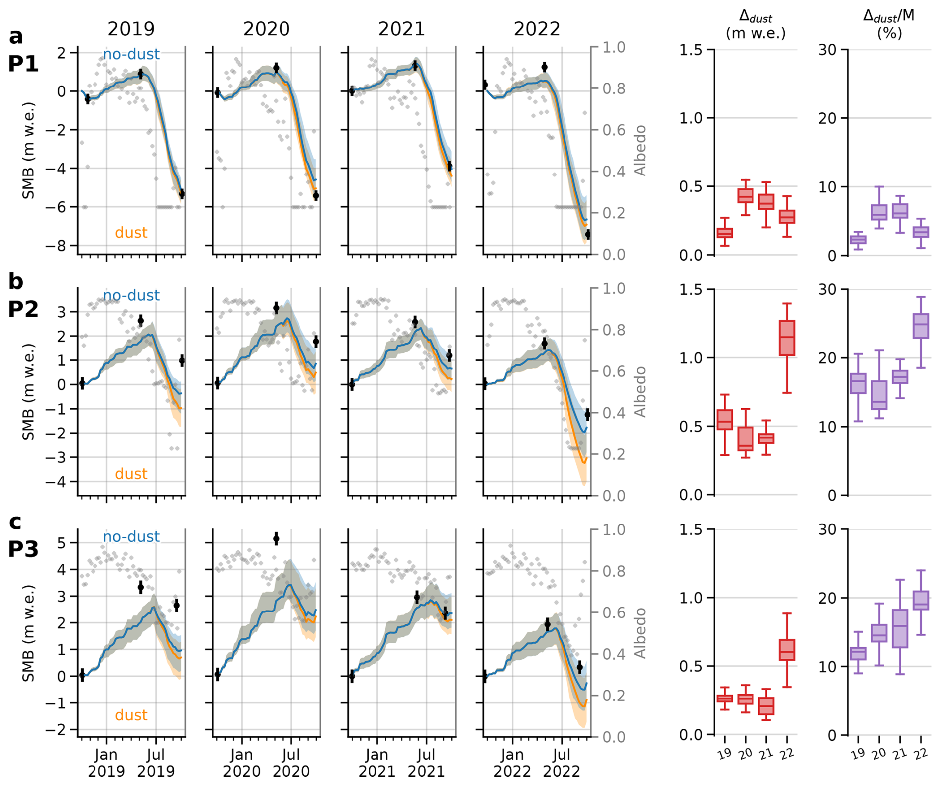
Figure 5 SMB evolution and albedo (dots) at noon for hydrological years 2019 to 2022 at three different locations. Median (solid line) and Q10–Q90 of the 40 ensemble members for dust and no-dust simulations. Black points and lines are the observed SMB and their uncertainty using the nearest measurement point. Δ_dust (m w.e.) is the difference in SMB between the simulation with and without mineral dust, and ${\mathrm{\Delta }}_{\text{dust}}/\text{M}$ (%) is the ratio between Δ_dust and the total melt. P1 was in the ablation area (2400 m a.s.l.), P2 near the equilibrum-line elevation (2900 m a.s.l.) and P3 in the accumulation area (3500 m a.s.l.), see Fig. 1d for precise locations. SMB scale is different at each location. Double digits refers to the years.

At point P1 in the ablation area, the annual simulated SMB was negative for all years from 2019 to 2022 (orange curve in Fig. 5). Without mineral dust, the simulated annual SMB was still largely negative (blue curve in Fig. 5). The difference in annual SMB for the simulations with and without dust in snow Δ_dust remained below 0.6 m w.e. for all years. The fraction of melt due to dust ${\mathrm{\Delta }}_{\text{dust}}/\text{M}$ was less than 10 %. The number of days with ice at the surface was between 60 and 140 d depending on the year, and the difference of time with ice exposed at the surface taking into account or not the impact of dust was lower than 10 d. At point P3, at the top of the accumulation area, the simulated annual SMB was positive for all years except 2022. At this point, the impact of mineral dust accounted for less than 0.3 m w.e. for each year in the period 2019–2021, and for less than 0.9 m w.e. in 2022. It represented between 0 and 25 % of the total melt. Ice was never exposed at this point. At point P2, near the end-of-summer snowline, the simulated annual SMB was either positive (2020, 2021) or negative (2019, 2022). This allowed, or not, the formation of a firn layer depending on the year. For years 2019, 2020 and 2021, the dust impact at P2 ranged from 0.25 to 0.75 m w.e. For 2022, the dust impact was 1.15 m w.e. [0.90, 1.34] (median, Q10–Q90), which represent 24.6 % [19.1, 27.3] of the total melt. In 2022, ice was exposed during 42 d in the simulation that takes dust into account.

The spread of the ensemble for the dust impact varied depending on the location and the year. For instance, there was a small ensemble spread in dust impacts Δ_dust, e.g., at P1 with all Δ_dust ranging within ±0.3 m w.e. for each year, compared to P2 with a higher ensemble spread, e.g., with Δ_dust ranging between 0.75 and 1.4 m w.e. in 2022. However, this spread of dust impact is always lower than the spread of annual SMB induced by the meteorological ensemble, that is always larger than 1 m w.e. For the three points, we observed that the impact of dust was mainly effective during the summer. Indeed, for both simulations with and without dust, their winter accumulations in Fig. 5 were very similar, while the ensemble means of SMB gradually diverge during the summer melt.

3.2.2 At the glacier scale

At the glacier scale, the simulated dust impact on the annual SMB was higher in 2022 than in previous years, in agreement with results at the three locations P1, P2 and P3. For years 2019 to 2021, the median [Q10–Q90] of the annual SMB decrease due to dust at the glacier scale were 0.31 m w.e. [0.29, 0.35], 0.42 m w.e. [0.39, 0.47], and 0.45 m w.e. [0.41, 0.49], respectively, representing 9.1 % [8.3, 9.9], 12.5 % [11.8, 13.2], 14.8 % [13.4, 16.1] of the total annual melt. However, in 2022, the impact due to dust in snow and firn rose to 0.63 m w.e. [0.54, 0.69] representing 13.2 % [11.8, 14.7] of the total melt. In 2022, the albedo averaged over the whole glacier at noon over the year decreased by 0.03 [0.028, 0.033] due to dust. When restricted to summer 2022, from May to September, snow albedo decreased by 0.062 [0.056, 0.067].

Overall, when looking at each point simulation, we found very different dust impacts over the glacier depending on the location, from almost 0 to above 1 m w.e., due to very different impact of dust on snow summer albedo (summer albedo decreased from 0 to 0.12 depending on the location, see Appendix Fig. E2). When comparing each year, for all simulation points, the dust impacts from year 2019 to 2021 were mostly lower than that of 2022 in the accumulation area (Appendix Fig. E1).

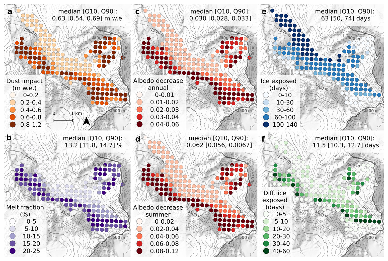
Figure 6 At each simulation point for hydrological year 2022 (1 October 2021 to 30 September 2022): (a) Dust impact Δ_dust, i.e., difference in simulated SMB for dust and no-dust. (b) Melt fraction ${\mathrm{\Delta }}_{\text{dust}}/\text{M}$, i.e., fraction of the melt due to dust. (c) Annual albedo decrease due to dust. (d) Summer albedo decrease due to dust. (e) Number of days with ice exposed at the surface for the dust simulation. (f) Number of days with ice exposed for the dust simulation, but not for the no-dust simulations. The colors represent the median of the ensemble at each point. The aggregated value refers to the median and [Q10–Q90] range (over the 40 members) of the mean over all simulation points. Background map from MapTiler.

Thereafter, we focus on the year 2022, as it presents the highest dust impacts. However, the values for the complete period 2019–2022 are presented in Appendix Figs. E1, E2 and E3. Figure 6 illustrates the spatial distribution of the simulated dust impacts in 2022. The dust impact presented a high spatial variability, ranging from 0 to 1.2 m w.e., was lower below the end-of-summer snowline of 2021 and in the upper part of the accumulation area. Although the dust impact values in 2022 at higher elevations were close to the value at lower elevations (Δ_dust between 0.2 and 0.6 m w.e.), the melt fraction at higher elevations was much higher (${\mathrm{\Delta }}_{\text{dust}}/\text{M}>\mathrm{15}$ % at high elevation vs. ${\mathrm{\Delta }}_{\text{dust}}/\text{M}<\mathrm{5}$ % at lower elevations). In 2022, the highest impact of dust occurred around 3000 m a.s.l., which was just above the end-of-summer snowline of 2021 (Fig. 1a), and differed depending on the aspect: at 3000–3200 m a.s.l. for the north-eastern part of the glacier which is south-west facing, at 2900–3100 m a.s.l. for the top of the main tongue which is north facing, at 2900–3100 m a.s.l. for the western part of the glacier which is north-east facing.

The spatial pattern of the albedo reduction due to dust is similar to the spatial pattern of the dust impact (Fig. 6c and d), with a summer albedo decrease that is nearly the double of the annual albedo decrease. At the bottom of the main glacier tongue, numerous simulation points had ice exposed at the surface for more than 100 d in 2022 (Fig. 6e). Almost all points below the 2021 end-of-summer snowline had ice at the surface for more than two months. The points with the longer time duration with ice at the surface in the dust simulation, but snow/firn in the no-dust simulation, were located near the end-of-season snowline of 2021 (Fig. 6e) with up to 40–50 d of difference. At the bottom of the main tongue, this time duration dropped to less than 5 d difference.

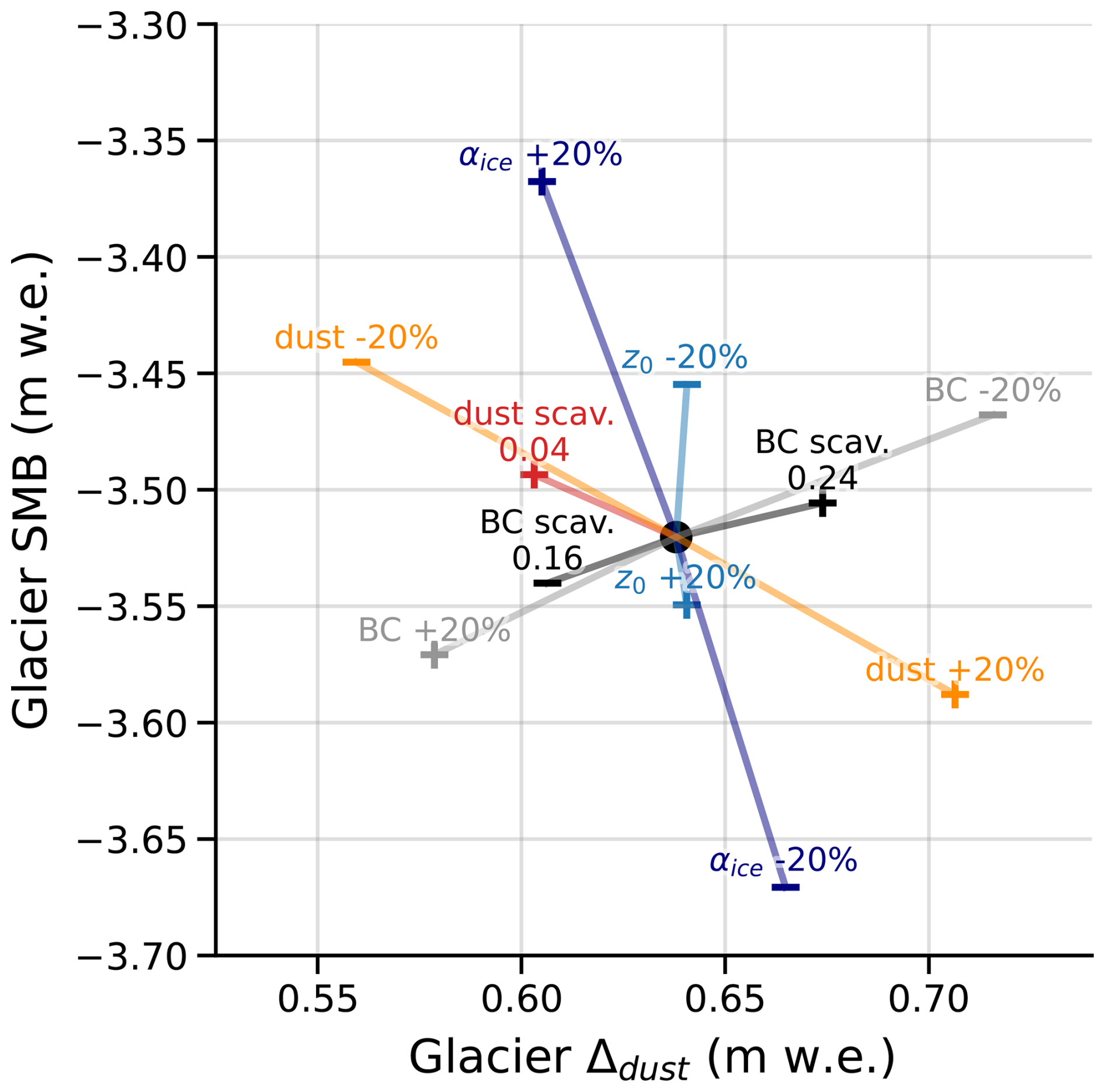
Figure 7 Sensitivity of glacier-wide annual SMB (y axis) and dust impact Δ_dust (x axis) to forcing inputs and model parameters relative to the reference simulation (central black dot) for hydrological year 2022.

3.3 Sensitivity analysis

We investigated the sensitivity of the principal inputs and model parameters to understand how different values of our inputs and model parameters can affect the results. We investigated the impact of ice albedo modifications (±20 %), roughness length (±20 %), BC scavenging efficiencies (±20 %), mineral dust scavenging efficiency (0.04 and 0.2 instead of 0), dust and BC deposition fluxes (±20 %). Figure 7 shows the difference caused by these modifications on: (i) the annual glacier SMB; and (ii) the estimated dust impact Δ_dust at the glacier scale in 2022. Increasing (decreasing) ice albedo by 20 % increased (decreased) the annual glacier SMB by around 0.14 m w.e. For the roughness length, an increase (decrease) of 20 % increased (decreased) the annual glacier SMB by around 0.03–0.08 m w.e. Modifications on ice albedo or roughness length modified the dust impact by less than 0.04 m w.e. An increase (decrease) in dust and BC input fluxes lowered (increased) the annual glacier SMB by around 0.05 m w.e., hence the model has the same sensitivity to both LAP deposition fluxes. Moreover, increasing (decreasing) dust input fluxes increased (decreased) the dust impact by 0.08 m w.e. An increase in scavenging efficiencies, which lowers the impurity accumulation at the snow surface, increased the annual glacier SMB. Overall, these results showed that the sensitivity of the dust impact to dust or BC deposition fluxes was larger than the sensitivity to their respective scavenging coefficients and to other parameters of the model such as the ice albedo and the roughness length. We finally observed that the glacier SMB and dust impacts resulting from the sensitivity tests described previously were included in the ensemble spread (see Fig. 8), hence included in the meteorological uncertainty. Specifically, for glacier SMB, the meteorological uncertainty was much wider than the spread of all the sensitivity tests described above, whereas for glacier dust impact, the meteorological uncertainty was a bit larger than a variation of ± 20 % of dust inputs. Nevertheless, these sensitivities do not represent the impact of the uncertainties of each input and parameter, that are later discussed in Sect. 4.

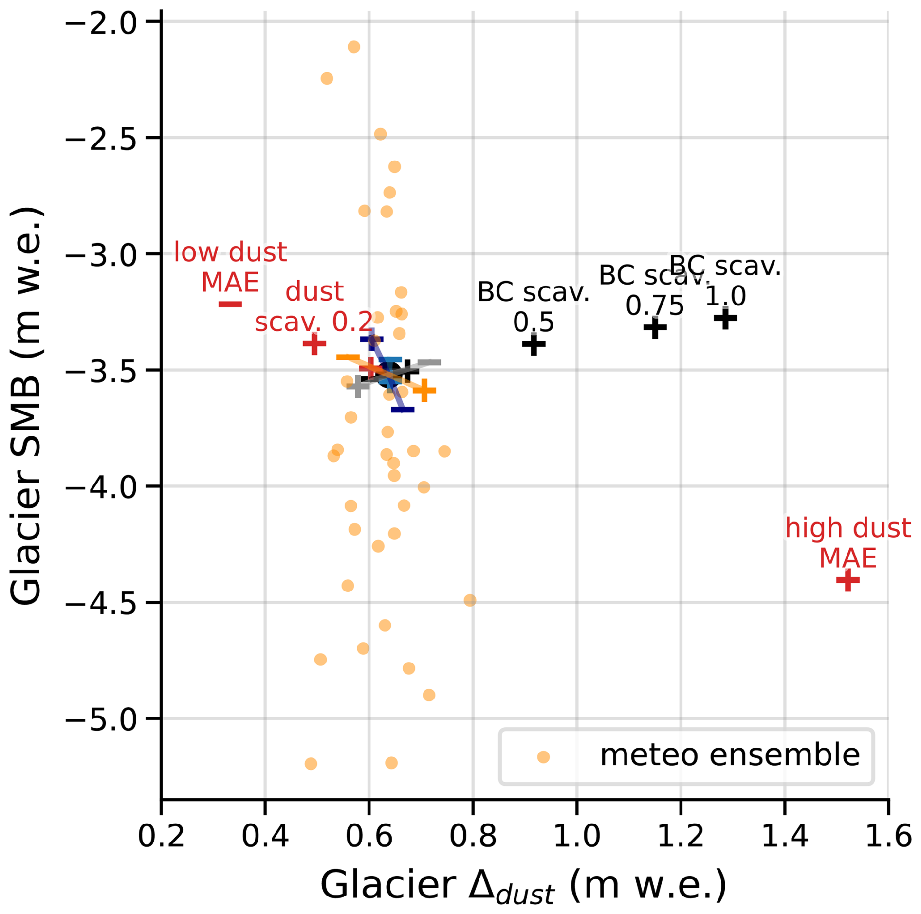
Figure 8 Impact of uncertainties relative to LAP scavenging efficiencies and deposition fluxes on the glacier-wide annual SMB (y axis) and dust impact Δ_dust (x axis) for hydrological year 2022. Reference simulation is represented by the central black dot. The 40 members of the ensemble are represented with the orange dots.

In addition to this sensitivity analysis, and as the scavenging efficiency of BC is subject to large uncertainties (Sect. 4.2), we also tested much higher BC scavenging efficiencies k_BC of 0.5, 0.75 and 1.0 (Fig. 8). These BC scavenging efficiencies slightly lowered the annual glacier SMB by 0.15 to 0.30 m w.e. compared to the previous efficiencies. However, such BC scavenging efficiencies increased the impact of dust up to 1.3 m w.e. in the annual glacier SMB of 2022 compared to 0.63 m w.e. with the initial BC scavenging efficiency of 0.2. A dust impact of 1.3 m w.e. represented approximately 25 % of the total melt. Figure 8 shows that the sensitivity of the dust impact to BC scavenging efficiency is not linear. The growing impact of mineral dust with increasing BC scavenging efficiency is discussed in Sect. 4.2.

4 Discussion

In this study, we simulated the SMB of Argentière Glacier for four years with an advanced snow model that explicitly takes into account the impact of mineral dust and BC. At the glacier-wide scale, we showed that mineral dust lowered the annual SMB by up to 0.63 m w.e. [0.54, 0.69] in 2022, which represents 13 % [12, 15] of the total melt. At the point scale in specific areas of the glacier, the impact of mineral dust lowered the annual SMB up to 1.2 m w.e.

4.1 Role of dust

If the impact of mineral dust strongly varied with the location at the glacier surface, its deposition flux was homogeneous across the whole glacier. The results shown in Fig. 5 illustrate three different cases.

The first case corresponds to the ablation area where the annual SMB and the mean annual albedo with dust were lowered by 0–0.5 m w.e. and 0–0.02, respectively (Fig. 2a). Since we only simulated the impact of dust inside snow, and not on ice, two reasons explain these differences in SMB and albedo at lower elevation: (i) mineral dust lowers the albedo of the seasonal snow; and (ii) ice, which has a lower albedo than snow, is exposed earlier during the melt season, and acts as a positive feedback on melt. If we had also modelled the impact of dust on the ice surface, the dust impact in the ablation area would have likely been higher.

The second case corresponds to the accumulation area, where snow was always present at the glacier surface, and both annual SMB and albedo were lowered by 0.2–0.8 m w.e. and 0.02–0.04, respectively. In this case, snow from the winter does not completely melt, dust stays exposed at the surface during a long time period and leads to a higher melt fraction than at low elevation.

The third case corresponds to the area just above the end-of-summer snowline from previous years, when atmospheric conditions during the summer period lead to a negative annual SMB. In such a case, the firn layers from the previous years with accumulations of LAPs reappear at the surface, leading dust to lower the annual SMB and albedo by 0.8–1.2 m w.e. and 0.03–0.05, respectively. For instance at point P2, for most of the members the annual SMB was positive in 2020 and 2021, allowing the re-exposure of the accumulated LAPs in 2022, when the annual SMB was negative. This is also the scenario of Fig. 2b. This persistent impact of LAP over several years has already been mentioned by Gabbi et al. (2015) in the European Alps, and more recently by Möller et al. (2019) in Iceland. In such a scenario, we noted that the spread of dust impacts induced by the ensemble was larger, and this could be generalized to nearly all points above the end-of-summer snowline of 2021 (Appendix Fig. E1). This higher ensemble spread might be due to: (i) a longer exposition of dust at the snow surface, with different shortwave radiation conditions depending on the ensemble member; (ii) a larger diversity of scenarios, with ice exposed during the summer for some members, and only firn exposed for other members. To sum up, mineral dust has varying impacts and uncertainty depending on the location on the glacier and the time of the year, with a maximum impact of dust found close to the end-of-summer snowline. Such an impact variability could only be found using a fine horizontal spatial resolution, here 250 m.

At the glacier scale, our results for Argentière Glacier showed that the impact of dust on the glacier-wide annual SMB ranges between 0.31 and 0.63 m w.e. (medians) for the years 2019 to 2022, which was an order of magnitude higher than the mean annual dust impact of 0.03–0.06 m w.e. computed at two points over a century on Clariden Glacier by Gabbi et al. (2015). Such a difference may be explained by multiple factors. First, both studies focused on different time periods. Thus, the LAP deposition flux sources, which highly vary with time, were also different. For instance, the annual dust deposition fluxes present a high inter-annual variability (e.g., Di Mauro et al., 2015; Réveillet et al., 2022), and the annual BC deposition fluxes significantly decreased after the 1990s in the French Alps (e.g., Sun et al., 2020; Grange et al., 2020; Réveillet et al., 2022), which could explain a lower impact of BC and a higher impact of dust in the 21th century. Second, both studies focused on different geographic locations. Clariden Glacier is located in the northern part of the European Alps, that is less exposed to Saharan dust depositions. For instance, Dumont et al. (2023) showed that the deposited dust mass decreased with the distance to the source during a single Saharan dust deposition event, with less dust deposited in the Swiss Alps compared to the French Alps. Ultimately, the mass absorption efficiencies (MAE) of both studies were different. For BC, Gabbi et al. (2015) used a constant MAE_BC=6.8 m² g⁻¹, while for our simulations, we used a higher MAE_BC depending on the wavelength λ such as MAE_BC(λ)=7.5 m² g⁻¹, at 550 nm. We could not directly compare the MAE of dust, since Gabbi et al. (2015) used a MAE of Fe-oxides and we used a MAE of mineral dust. However, we computed the broadband ratio $({\text{MAE}}_{\text{BC}}\times m_{\text{BC}})/({\text{MAE}}_{\text{dust}}\times m_{\text{dust}})$ with m_LAP the mean annual deposited mass of each LAP. For Gabbi et al. (2015), this ratio was close to 10, i.e., BC has potentially more impact than dust. This is in line with their results showing that the reduction of the SMB by BC is an order of magnitude higher than that of dust. For our study, this ratio was close to 1, i.e., dust and BC have potentially the same impact in case no scavenging is taken into account. Besides other model and input differences, this could partially explain that the dust impact of this study is higher than that of Gabbi et al. (2015) by an order of magnitude.

The range of uncertainty was inferred by a meteorological ensemble, and in 2022, the obtained range was [0.54, 0.69] m w.e. When varying the dust deposition flux by ±20 %, the resulting uncertainty is included in the previous range. We found a spatial variability of 2σ≈45 % on the dust deposition fluxes around the selected point of the ALADIN grid (Sect. 2.3), that the meteorological ensemble does not take into account. However, the impact of the dust deposition uncertainty has likely the same order of magnitude than the impact of the meteorological uncertainty (≈0.1 m w.e. in 2022).

The dust scavenging efficiency k_dust that was set to 0 in the reference version, i.e., no scavenging of dust (see Sect. 2.4.1). A higher k_dust=0.04 led to a lower impact of dust (Fig. 7). Although this was poorly documented in the existing literature, we suspected that dust scavenging efficiency at the snow surface could be significantly higher than the previous sensitivity test. So we added a test of uncertainty using $k_{\text{dust}}=\mathrm{0.2}=k_{\text{BC}}$ (Fig. 8), which is likely too high since BC particles scavenge more easily than large particles such as dust (e.g., Conway et al., 1996; Doherty et al., 2013). The dust impacts using those two dust scavenging efficiencies were still inside the uncertainty induced by the meteorological ensemble.

The MAE of dust used in this study was slightly lower than initial values used in previous studies in the framework of a seasonal alpine snowpack at intermediate elevations (Tuzet et al., 2020; Réveillet et al., 2022). The reliability of this parametrization was assessed by the evaluations of section 3.1 and the evaluation of the modelled snow albedo in Appendix Fig. B3. Such lower MAE implicitly accounts for the probable aggregation of LAP (likely due their high concentrations during long melt seasons) that lowers the MAE (e.g., Bond and Bergstrom, 2006; Schwarz et al., 2013). In addition, the temporal variability of the absorption efficiency of dust was not represented in the model: the MAE used in this study was constant in time. However, the absorption efficiency of mineral dust can vary for each deposition event depending on the region of origin or the size distribution (e.g., Dumont et al., 2023; Caponi et al., 2017), as well as by its location within the snowpack either inside or outside the snow grains (He et al., 2018) and by the aggregation state of the dust particles (Bond and Bergstrom, 2006). As shown in Fig. 8, a low and a high value of dust MAE (Sect. 2.4.1) strongly affects the resulting dust impact (Δ_dust<0.4 m w.e. for the low MAE and Δ_dust>1.4 m w.e. for a high MAE). However, these extreme dust impacts are unlikely since the simulations using extreme dust MAE (low and high) results in degraded accuracy metrics with respect to in situ measurements compared to the reference scenario used throughout the study (not shown).

Finally, the maximum dust impact Δ_dust in our study was found in 2022. Given the extreme dust deposition event of February 2021 (Dumont et al., 2023), it might be surprising that the impact of dust in 2021 was lower than that of 2022. This shows that the impact of dust on the annual glacier SMB is not solely guided by the mass of dust deposited during the current year. Indeed, in 2021, a total of 15.1 g m⁻² of dust was deposited, whereas 13.1 g m⁻² was deposited during year 2022, and the simulated dust impact Δ_dust at the glacier scale was 0.45 m w.e. in 2021, and 0.63 m w.e. in 2022. The impact of dust on the annual SMB results from a combination of factors including the meteorological conditions, the timing of dust deposition and the time duration of exposure at the snow surface. For the extreme melt of 2022, the abnormally hot temperatures since May 2022, and numerous heatwaves during the summer 2022 probably strengthened the impact of dust by inducing an early and long exposure of dust on a part of the glacier. Moreover, the melt rate is also modulated by the reappearance of firn layers from previous years, e.g., the highly contaminated firn of 2021 during the 2022 melt season. To conclude, in the same way than the long-term evolution of a glacier depends on its evolution during the past decades, the impact of mineral dust is not limited to its recent history of deposition: mineral dust could act as a positive feedback for several years after deposition, particularly in the accumulation area.

4.2 Uncertainties linked to black carbon

The reference BC scavenging efficiency k_BC used by previous studies is 0.2 (e.g., Flanner et al., 2007; Gabbi et al., 2015), and we also chose this value in our reference simulation. Here, results showed that the sensitivity of the annual glacier SMB and dust impact to k_BC around 0.2 (±20 %) were two times lower than the sensitivity to BC deposition fluxes (±20 %) for year 2022 (Fig. 7). In other words, the intensity of BC deposition fluxes had here more influence on the annual glacier SMB and dust impact than the scavenging efficiencies. For the SMB sensitivity, this result was different than in Gabbi et al. (2015) who found an absolute sensitivity to BC scavenging efficiency three times larger than to BC deposition fluxes. We noted that different time steps may explain such a difference depending on the numerical scheme (15 min in our study, 1 d in Gabbi et al., 2015).

Furthermore, multiple studies reported that k_BC is subject to large uncertainties: k_BC∈ [0.003, 2.0] depending on the BC species in Flanner et al. (2007), k_BC∈ [0.02, 2.0] in Bond et al. (2013), k_BC∈ [0.02, 2.0] in Qian et al. (2014). Thus, we conducted a more detailed sensitivity study at the glacier scale by increasing k_BC from 0.2 to 1.0. Figure 8 illustrates that the associated annual glacier SMBs were still within the spread of the ensemble, with an increase in annual glacier SMB of 0.15–0.3 m w.e. that was small compared to a SMB of less than 3 m w.e. We also noted that this increase in glacier SMB was not linear with regard to k_BC, as demonstrated by Dumont et al. (2020) for the relationship between the shortening of the snow melt period and the deposited mass of mineral dust. More importantly, the dust impact was significantly modified without modifying the dust deposition fluxes: increasing k_BC from 0.2 to 1.0 doubled the dust impact from 0.63 to 1.3 m w.e. and the resulting dust impacts were not in the ensemble spread anymore. The reason behind this comes from the dependency of albedo on dust and BC, as shown in Eqs. (3) and (7) in Tuzet et al. (2020): the derivative of snow albedo with regard to dust concentration, that is negative, is an increasing function of BC concentration. Hence, higher BC scavenging efficiencies lead to less BC at the snow surface, and to higher dust impacts.

Overall, the uncertainties on LAP scavenging efficiencies in snow result in large uncertainties on the respective absolute impacts of dust and BC. This highlights the need to better understand the motion of the different LAPs inside of the snowpack at the micro-scale. Here, BC scavenging in snow, that is still not quantified properly in the European Alps, represents a significant source of uncertainty on the dust impact. However, our simulations estimated the respective impact of each impurity for varying scavenging efficiencies, showing that an increase in the simulated BC scavenging efficiency led to a higher simulated impact of dust.

4.3 Other limitations

Although we believe that our study contributes to a better understanding of the role of LAPs on the glacier SMB, our simulations were subject to multiple other limitations that are discussed below.

The values of ice albedo and roughness length were taken constant in time and space, while numerous studies showed that those parameters could vary significantly in time and across a glacier (e.g., Brock et al., 2006; Oerlemans et al., 2009; Naegeli and Huss, 2017). However, the sensitivity study of Sect. 3.3 shows that although changing ice albedo values can moderately modify the glacier SMB, this only slightly modifies the dust impact at the glacier scale compared to other sensitivity tests, e.g., mineral dust and BC deposition fluxes. Given that the uncertainty in ice albedo was estimated to be around 20 % of its reference value (Sect. 2.2.5), the assumption of taking a constant ice albedo does not impact the conclusions of the present study. For the roughness length, its value can vary by an order of magnitude, but the sensitivity of glacier dust impact to roughness length is negligible, so taking a constant roughness length value does not modify the conclusion of this study.

The evaluation of the simulated SMB against point measurements and S2 images shows that the spread of simulated SMB was large and covers a wide range of scenarios, although this appears necessary to cover uncertainties at each measurement point. In the accumulation area, the RMSE of the summer melt against point measurements are of the same order of magnitude than that at lower elevation, but the summer melt is lower, resulting in larger relative uncertainties. However, the point measurements in the accumulation area are subject to larger uncertainties due to: (i) preferential accumulation, or (ii) human errors in distinguishing seasonal snow from old firn and measuring large snow accumulations. For instance, the measurement location associated with point P3 is known to be located in an area with preferential snow accumulation (which results in an observed SMB often higher than the simulated SMB in Fig. 5c). Such a measurement may then not be representative of the 250 by 250 m surrounding area.

The spatially distributed evaluation of the simulation against the Pléiades-derived SMB showed that the spread of the simulated SMB was not sufficient to capture the highest snow accumulation at the base of the north-east facing headwalls. This low accumulation at the base of the headwalls translated into a lower simulated SMB at the glacier scale, e.g., −1.9 m w.e. yr⁻¹ simulated vs. −0.59 m w.e. yr⁻¹ for the Pléiades SMB over the period 2018–2022. Steep surrounding slopes are known to be prone to frequent avalanches from the headwalls onto the Argentière Glacier as demonstrated by Kneib et al. (2024a). To account for avalanches, one could argue that we could have artificially amplified precipitations, e.g., using a simple avalanche model like Snowslide (Bernhardt and Schulz, 2010), which may lead to better evaluation results. But at the same time, it is highly unclear how LAPs redistribute within the snow during such events. Are they redistributed? If so, do they redistribute homogeneously, at the top or under the transported snow? Because of a lack of knowledge regarding those issues, we did not model this process. To sum up, our simulation lacked snow accumulation at the base of the headwalls, presumably due to avalanches, therefore the results at these particular locations need to be taken with caution, and this could slightly modulate the dust impact at the glacier scale.

Other LAPs than mineral dust and BC in snow might also impact glacier albedo. Red snow algae are known to lower snow albedo in spring and summer in the European Alps (e.g., Ezzedine et al., 2023). However, Roussel et al. (2024) have shown that their presence over Argentière Glacier was very limited. Indeed, the total area with at least one retrieval of red algal blooms over the period 2018–2022 represents less than 1 % of the area of the Argentière Glacier. Based on this, we did not consider snow algae in this study, because their impact would have been small compared to other LAPs. Brown carbon is also known to increase light absorption in the snowpack. Its optical properties, atmospheric concentrations and deposition fluxes are still under large uncertainties, however we believe that the impact of brown carbon is lower than that of BC (Skiles et al., 2018). In addition, mineral dust from local sources, e.g., surrounding moraines, might also contribute to lower the glacier albedo (e.g., Oerlemans et al., 2009). On annual snow, however, we assumed that their impact was relatively small compared to dust and BC.

The uncertainties in the results can also be related to the choice of the model and the parameters used in the model (e.g., Lafaysse et al., 2017). In this study, this primarily concerns the physical processes driving snow evolution and the radiative transfer model. Concerning the radiative transfer model, here TARTES coupled with the snow model, comparisons between radiative models (SNICAR and TARTES in Picard and Libois, 2024) indicate that the choice of the radiative transfer model has a significantly smaller impact on the results than variations in the optical properties of the LAP, here represented using the MAE of each LAP. Therefore, the uncertainty related to the radiative model is fully accounted for in this study by varying the dust MAE factor (Sect. 4.1). Concerning the snow model, an ensemble approach can provide estimates of snow model uncertainties. Réveillet et al. (2022) applied this method to Crocus and reported results on the impact of the LAPs comparable to deterministic simulations (supplementary Fig. S10 of Réveillet et al., 2022). Furthermore, uncertainties related to the snow model choice are generally smaller than those associated with the forcing (e.g., Etchevers et al., 2004; Günther et al., 2019). To explore the uncertainties related to the meteorological variables, we did the choice to use an ensemble of forcing produced using stochastic perturbations on the adjusted SAFRAN data (Sect. 2.3.6). Ultimately, the dust impact presented in this study is expressed as relative differences between simulations rather than as absolute values, which limits the influence of uncertainties related to the forcing and to the snow model choice.

Finally, the deposition of LAPs was constant in space in this study. As underlined by Warren (2019), there is still a lack of knowledge about the heterogeneity of LAPs deposition at the small scale depending on topographic characteristics. For example, in the European Alps during the extreme dust event of February 2021, Dumont et al. (2023) showed that south-facing slopes had received higher dust quantities by up to one order of magnitude compared to other orientations, probably due to the trajectory of the dust transport coming from the South during this event. These preferential depositions were not taken into account in our simulations and further research will be needed to understand their impacts. Nevertheless, we may expect a higher impact of dust on south-facing slopes because of: (i) higher dust deposition; and (ii) higher shortwave radiation. Finally, one may also wonder whether the deposited quantities of LAPs are the same at all elevations.

Besides those modelling limitations, an extension of this method to other glaciers would also rely on the availability of computational cost and resource usage. In this study, the simulations with the snowpack model SURFEX/ISBA-Crocus, including 2×40 members (with and without dust) and around 40 sensitivity tests over the period 2008–2022 with 179 distributed points, lasted 0.75 h parallelized on 15 360 CPU (total of 480 d of CPU time), needed around 100 MJ, i.e., around 25 kWh, and emitted approximately 6 kg of CO₂ equivalent.

5 Conclusions

Here, we simulated the SMB of the Argentière Glacier during the years 2019–2022, ending with the exceptional melt of 2022 in the European Alps. We used the SAFRAN meteorological reanalysis adjusted with local observations and the LAP deposition fluxes from ALADIN as inputs for the SURFEX/ISBA-Crocus snow model at 250 m horizontal resolution. The resulting SMBs were evaluated using various data: summer point SMB measurements, Sentinel-2 images and Pléiades-derived distributed SMB. Embedded in the snow model, a radiative transfer model enabled quantifying accurately the impact of mineral dust inside snow.

For years 2019–2021, the lowering of the glacier-wide annual SMB due to mineral dust was between 0.31–0.45 m w.e. [0.30, 0.49], representing 9.1 %–14.7 % [8.3, 16.1] of the total annual melt. However, during the exceptional melt of 2022 the impact of dust increased to 0.63 m w.e. [0.54, 0.69] representing 13.2 % [11.8, 14.7] of the total melt. This year, depending on the location on the Argentière Glacier, LAPs had very different impacts on the SMB: between 0–0.5 m w.e. in the ablation area where ice was exposed during most of the melt season, between 0.4–0.8 m w.e. at higher elevation in the accumulation area where the glacier was permanently covered with snow, and the highest impacts, between 0.4–1.2 m w.e. were found in the vicinity of the end-of-summer snowline. At that latter location, the impact of mineral dust in 2022 rose up to 1.20 m w.e., representing more than 20 % of the total annual melt. We also showed that the impact of LAPs over the glacier was not simply correlated with recent depositions: due to melt, stacked LAPs in old buried firn layers from previous years could reappear at the snow surface, hence also contributing to lowering the albedo. This also means that the impact of LAPs is strongly modulated by meteorological conditions. Thus, taking LAPs into account in glacier melt requires a long-term memory both for the meteorological conditions and LAP deposition fluxes.

Our approach encountered some limitations at specific locations, such as at the base of the steep glacier headwalls where snow redistribution by avalanches strongly increases snow accumulation. Simulating this process would likely modify the simulated impact of dust at these locations. Furthermore, large uncertainties linked to the percolation of BC within the snowpack might lead to significantly higher impacts of dust. Using different mass absorption efficiency for the dust particles in snow also significantly modulated the results. Further research is needed to understand these processes and to quantify their impacts.

Since mineral dust in snow already accounts for around 8 %–16 % of the total annual melt for the Argentière Glacier for the period 2019–2022, its impact can not be totally neglected in past simulations and for future projections. Moreover, if we had considered mineral dust in ice, the impact on the surface mass balance could be higher. While quantifying the impact of LAPs locally and at a given date can be achieved using observation, modelling is required to estimate the past and future impact of LAPs over large spatial and temporal scales. The simulation setup of this study is easily transferable in time and space for glaciers where measurements of winter solid precipitation and summer melt exist. An automatic weather station is also useful to ensure the accuracy of the meteorological forcings used in the model. As a result, this work paves the way towards a comprehensive regional assessment of the impacts of LAPs on glaciers in monitored regions.

Appendix A: Data Appendix

Figure A1 Availability and usage of each data sources. Black lines show data usage.

Appendix B: Sentinel-2 Appendix

Table B1 Dates of the selected Sentinel-2 images.

Figure B1 Distribution of the S2 labelled pixels over Argentière Glacier depending on reflectance R_B4, and indexes NDSI and RGND. The thresholds mentioned in Sect. 2.2.3 are represented by the 3 black lines. See Sect. 2.2.3 for more details.

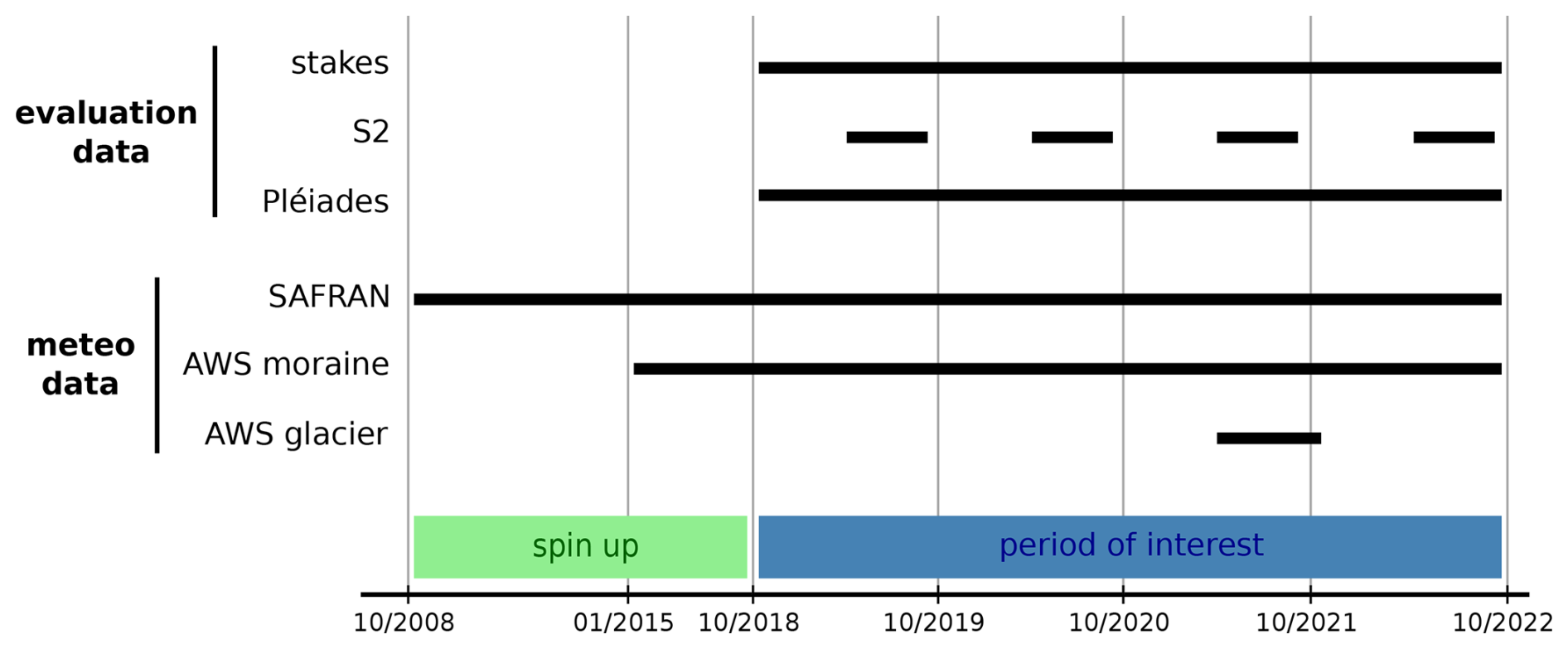
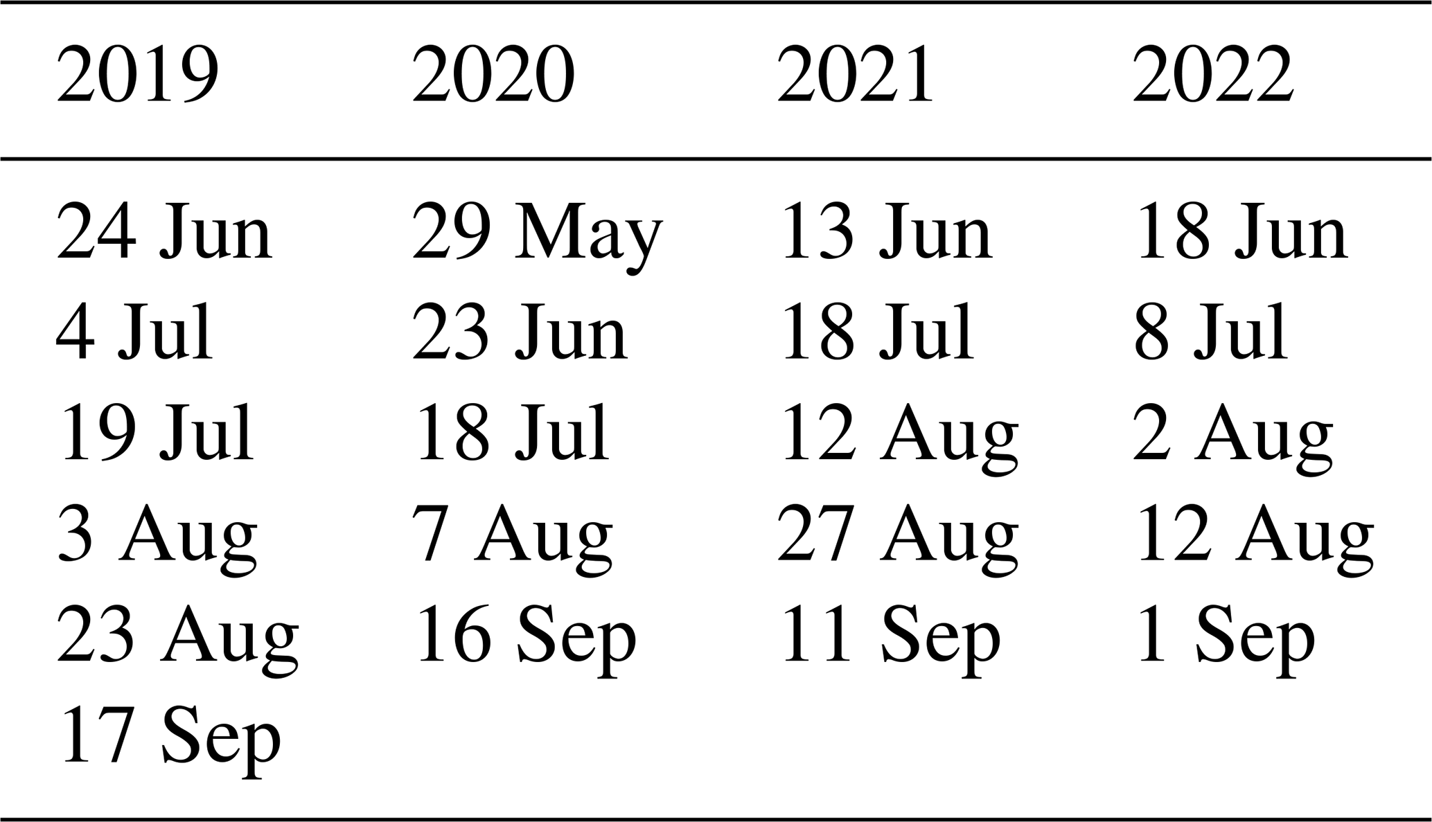
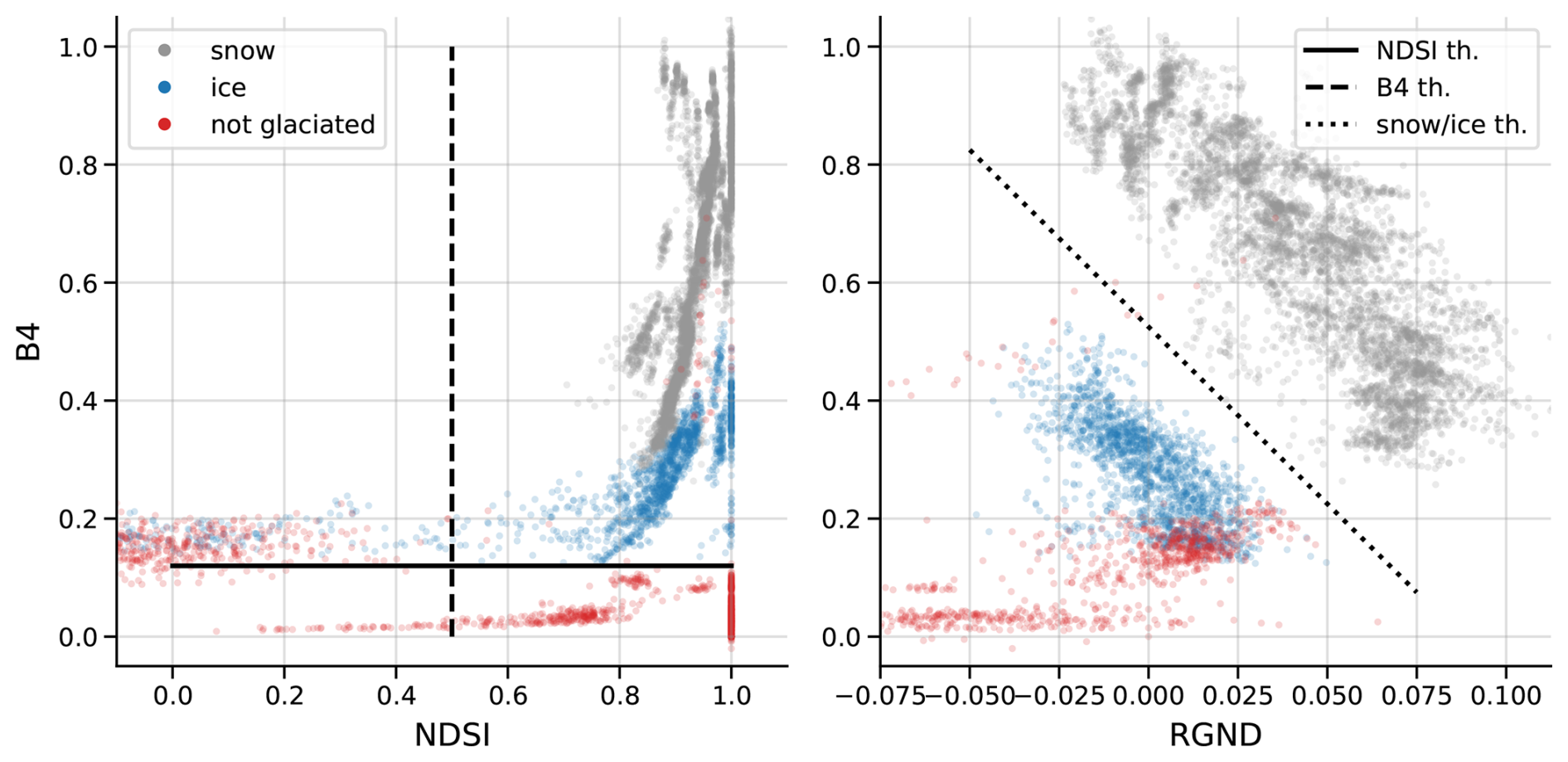
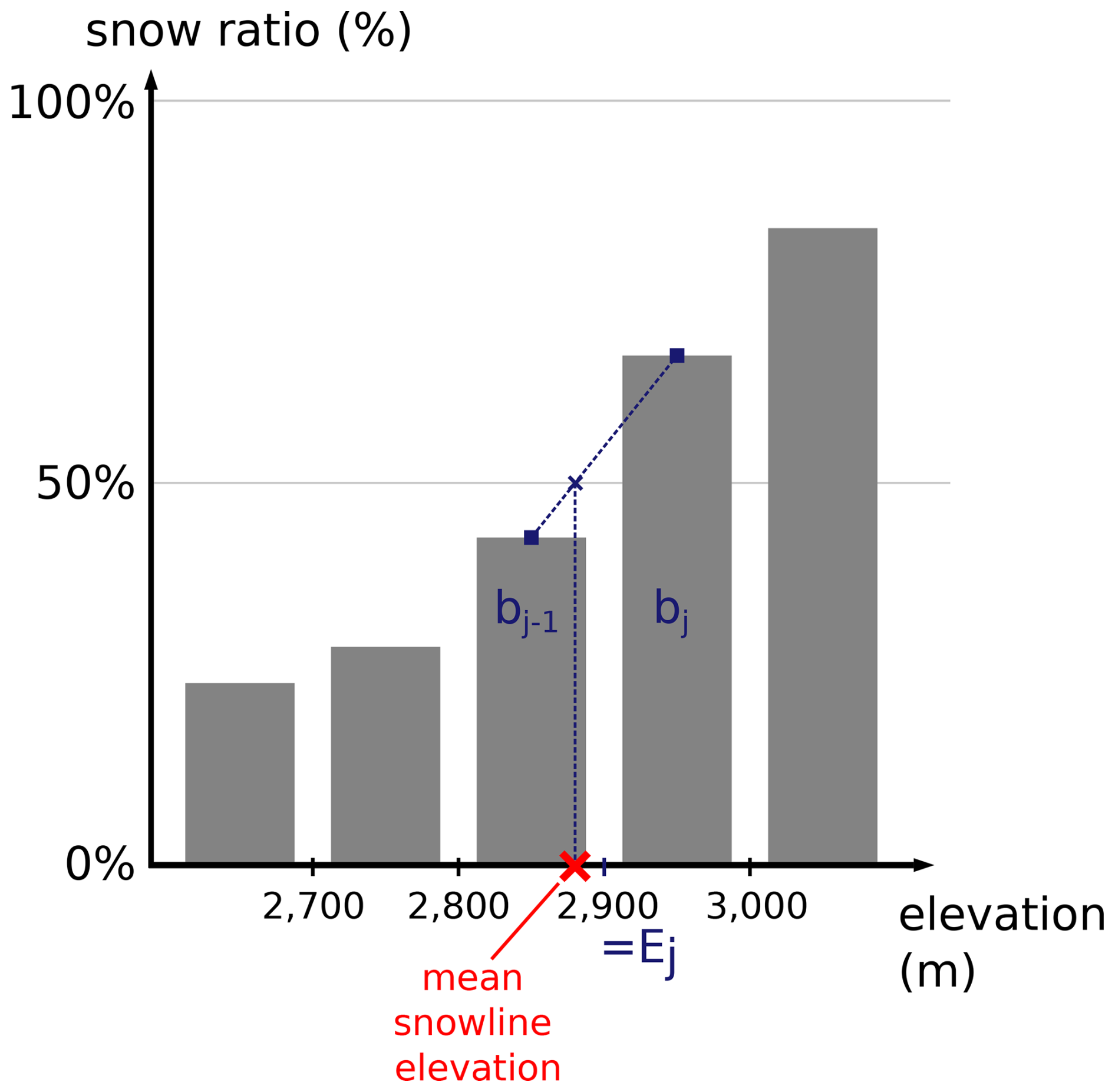
Figure B2 Illustration of the computation of the mean snowline elevation explained in Sect. 2.2.4.

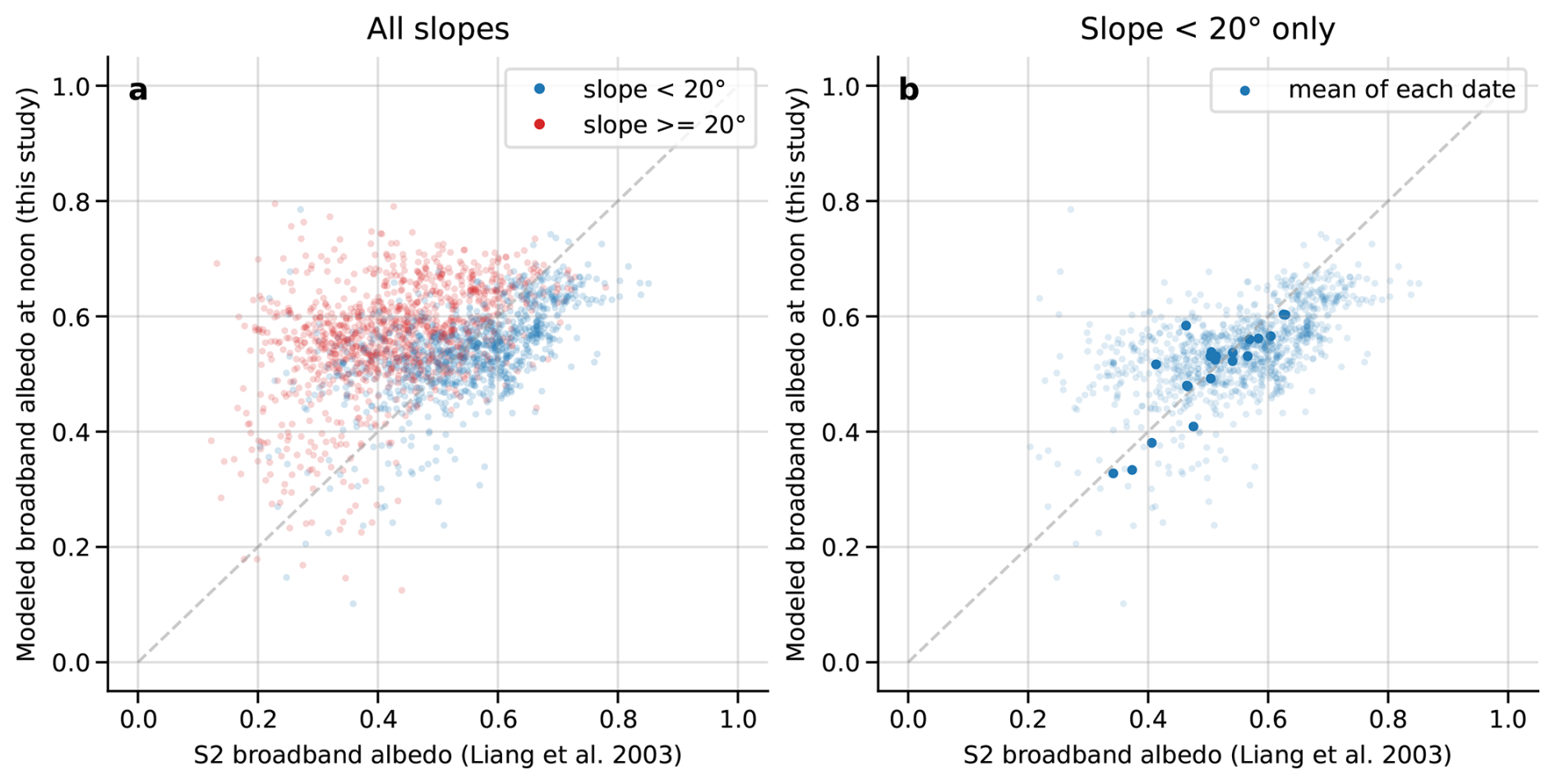
Figure B3 Comparison between simulated broadband albedo and broadband albedo derived from S2. See Sect. 2.2.6 for methods and limitations. (a) Influence of the slope. (b) Comparison for slopes <20°. The mean of all dates, except 2, shows less than 0.1 of difference between the modelled albedo and the albedo derived from S2. This comparison of broadband albedo has to be taken with cautious. Indeed, there are several limitations. First, the broadband albedo derived from S2 (Liang et al., 2003) was not developed for snow, an anisotropic surface (e.g., Dumont et al., 2010), i.e., the reflectance depends on the observation angle. Second, the uncertainties of the reflectance retrievals in complex terrain may be too high to estimate the accuracy of the simulated albedo, e.g., Cluzet et al. (2020), or panel (a) of this figure where the broadband albedo derived from S2 strongly depends on the slope.

Appendix C: Meteorological Appendix

Table C1 Sensors and the associated measurement accuracies for glacier and moraine AWSs.

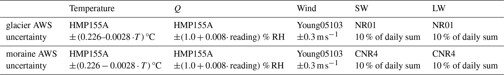
Table C2 Comparison between seasonal mean of SAFRAN variables at the location of the moraine AWS (1) and observed variables from the moraine AWS (2). For variables T (air temperature, K), W (wind speed, m s⁻¹), LW (incoming longwave, W m⁻², SW (incoming shortwave, W m⁻² during winter/summer periods (1 October, 1 May).

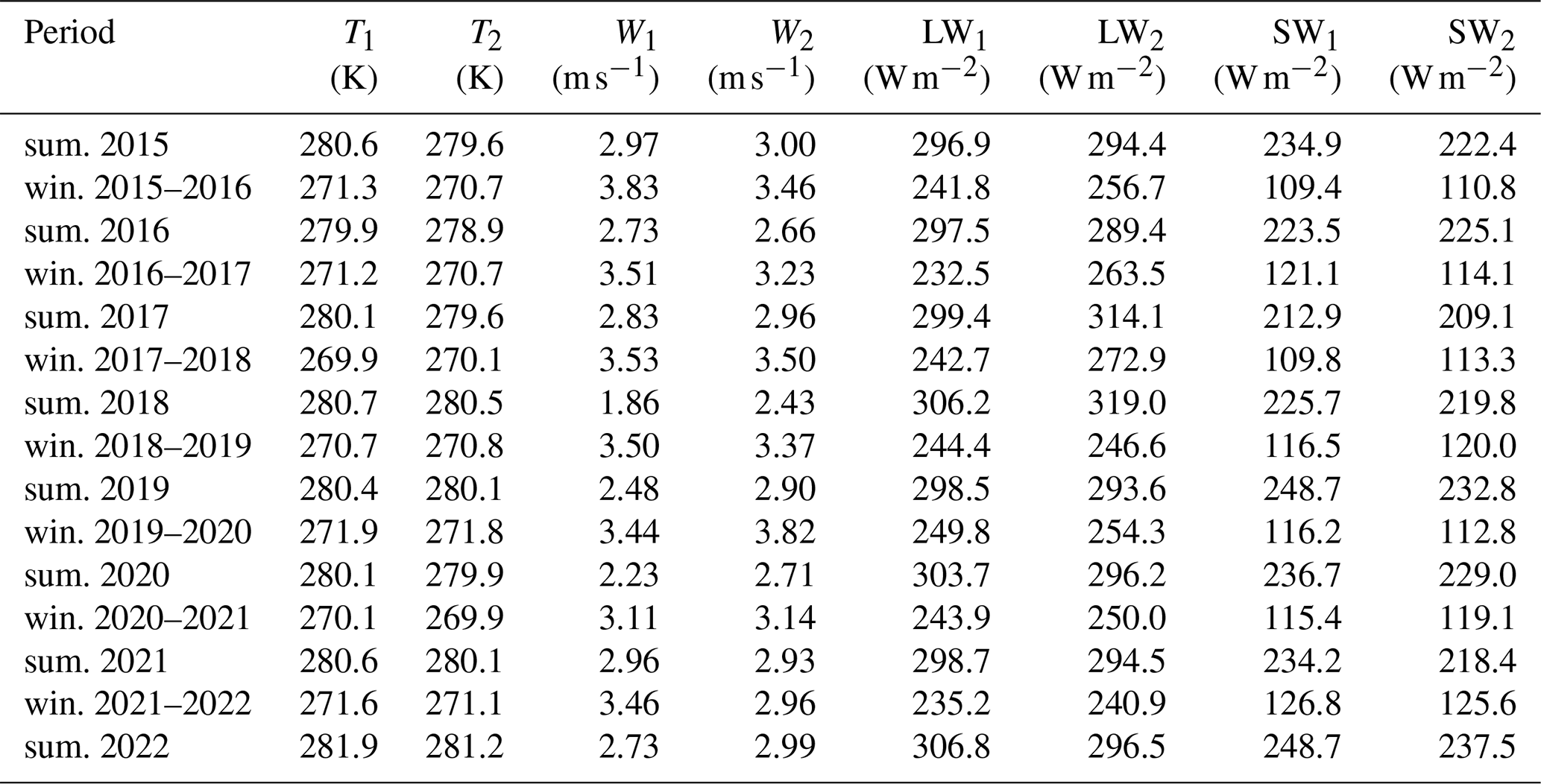
Stochastic perturbations of the meteorological forcings

The method is inspired from Charrois et al. (2016). Air temperature and longwave radiation are perturbed as additive variables, and shortwave radiation, wind and precipitations are perturbed as multiplicative variables. σ_X is estimated for each variable using the standard deviation of the difference between the modelled and the observed variable.

Given an additive variable V_t at time-step t, the perturbed variable $V_t^{*}$ is defined as

$$\begin{array}{}\text{(C1)}& V_t^{*}=V_t+X_t\end{array}$$

and in case the variable is multiplicative, $V_t^{*}$ is defined as

$$\begin{array}{}\text{(C2)}& V_t^{*}=V_t\cdot (\mathrm{1}+X_t)=V_t+V_t\cdot X_t\end{array}$$

In both cases, the perturbed term X_t is built using an autoregressive model of order one (AR(1))

$$\begin{array}{}\text{(C3)}& X_t=\mathit{\varphi }\cdot X_{t-\mathrm{1}}+{\mathit{ϵ}}_t\left({\mathit{\sigma }}_{\mathit{ϵ}}\right)\end{array}$$

with $\mathit{\varphi }=\exp (-\mathrm{d}t/\mathit{\tau })$, the times-step dt, the decorrelation time τ (such as τ>dt, and X_t is weak-sense stationary), and a white noise ϵ_t of variance ${\mathit{\sigma }}_{\mathit{ϵ}}^{\mathrm{2}}$. The parameter σ_ϵ could be retrieved for each variable.

For additive variables, by applying the variance to the perturbed term X of Eq. (C1), we find

$$\begin{array}{}\text{(C4)}& {\mathit{\sigma }}_{\mathit{ϵ}}=\sqrt{(\mathrm{1}-{\mathit{\varphi }}^{\mathrm{2}})}\cdot {\mathit{\sigma }}_X\end{array}$$

where σ_X is the standard deviation of X. In this case, σ_ϵ has the same dimension as X.

For multiplicative variables, by applying the variance to the perturbed term V⋅X of Eq. (C2), with X and V independents, and σ and μ the standard deviation and mean of a variable, we have

$$\begin{array}{}\text{(C5)}& {\mathit{\sigma }}_{V\cdot X}^{\mathrm{2}}={\mathit{\sigma }}_V^{\mathrm{2}}\cdot {\mathit{\sigma }}_X^{\mathrm{2}}+{\mathit{\sigma }}_V^{\mathrm{2}}\cdot {\mathit{\mu }}_X^{\mathrm{2}}+{\mathit{\sigma }}_X^{\mathrm{2}}\cdot {\mathit{\mu }}_V^{\mathrm{2}}\end{array}$$

with μ_X=0 and ${\mathit{\sigma }}_{\mathit{ϵ}}^{\mathrm{2}}=(\mathrm{1}-{\mathit{\varphi }}^{\mathrm{2}})\cdot {\mathit{\sigma }}_X^{\mathrm{2}}$, we find

$$\begin{array}{}\text{(C6)}& {\mathit{\sigma }}_{\mathit{ϵ}}=\sqrt{\mathrm{1}-{\mathit{\varphi }}^{\mathrm{2}}}\cdot {\displaystyle \frac{{\mathit{\sigma }}_X}{\sqrt{{\mathit{\sigma }}_V^{\mathrm{2}}+{\mathit{\mu }}_V^{\mathrm{2}}}}}\end{array}$$

In this case, σ_ϵ has no dimension.

In practice, for multiplicative variables, if the term (1+X_t) was lower than 0, the value of (1+X_t) was set to 0 to avoid setting negative values for meteorological variables such as wind or shortwave radiation. However, when the ratio $\frac{{\mathit{\sigma }}_X}{\sqrt{{\mathit{\sigma }}_V^{\mathrm{2}}+{\mathit{\mu }}_V^{\mathrm{2}}}}$ was higher than 0.42, (1+X_t) was set to 0 with a probability of around 1%. This was artificially increasing the mean of the perturbed variable. Hence, too avoid this behavior, we bounded the values of (1+X_t) between 0 and 2 (as in Charrois et al., 2016, that bounded (1+X_t) between 0.5 and 1.5).

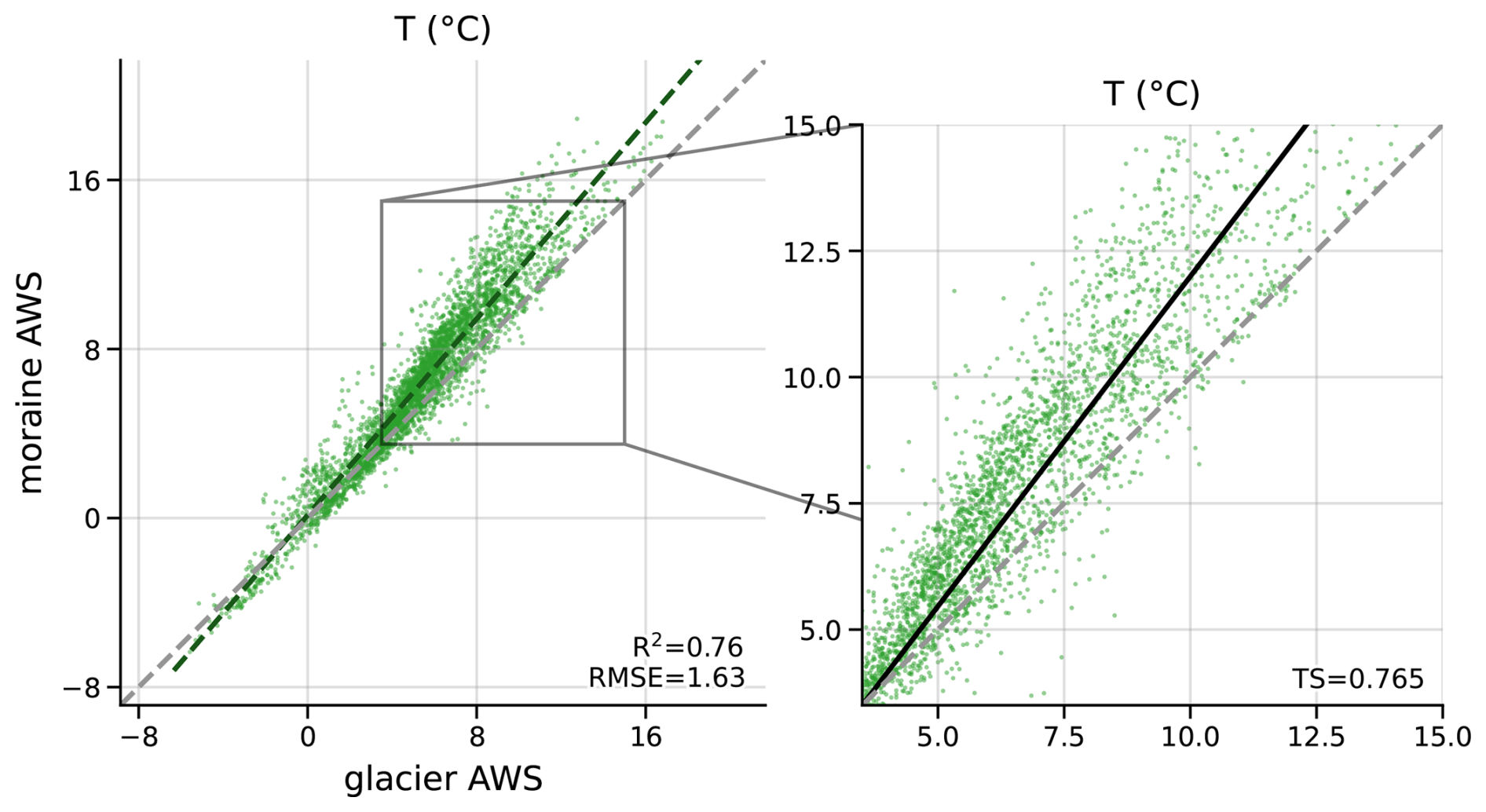
Figure C1 Comparison of the air temperatures between glacier and moraine AWS from 20 May 2021 to 22 October 2021. Grey dotted line represents 1:1 line. Colored dotted line represents the associated linear regression at all time-step. Zoomed plot shows air temperatures only above 3.5 °C. The solid green line is the linear regression with a zero intercept at 3.5 °C only for temperatures above 3.5 °C. TS is the the resulting temperature sensitivity.

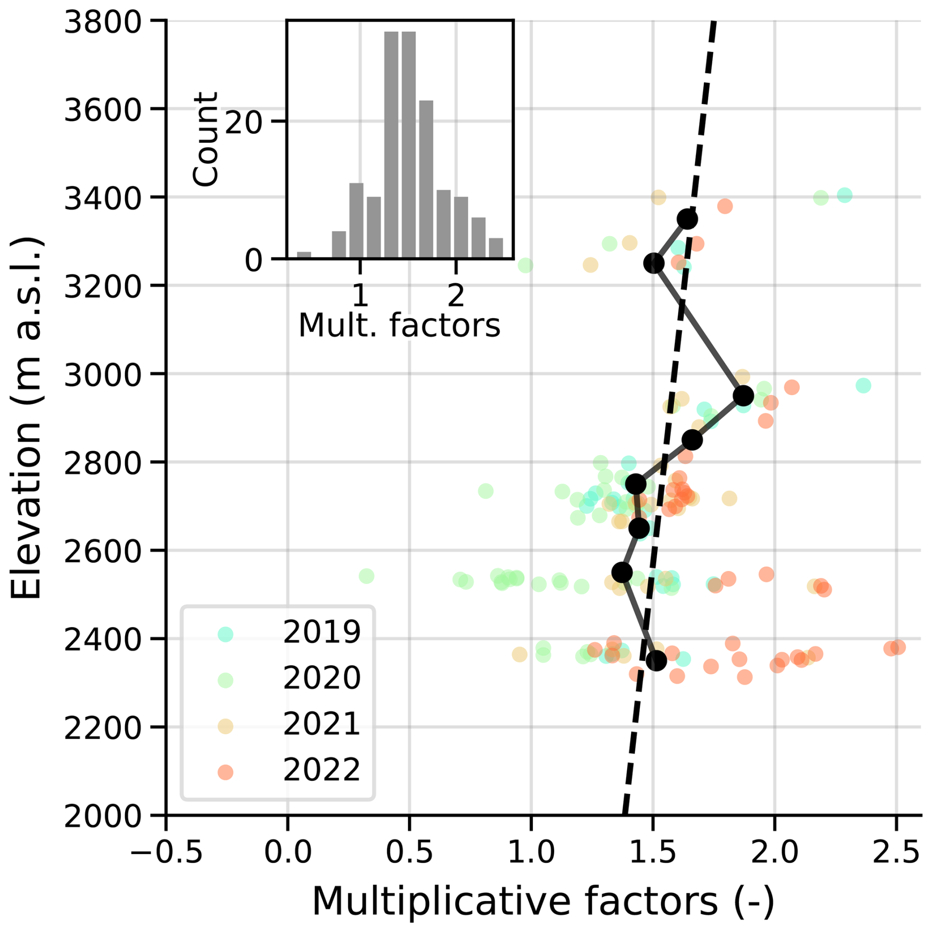
Figure C2 (a) Solid precipitation multiplicative factors, for each point accumulation measurements and four winter accumulations (colored dots), aggregated over 100 m bin (black dots), and linearly interpolated (dashed black line). Year N refers to winter accumulation between autumn N−1 to spring N. (b) Histogram of the multiplicative factors for each winter point accumulation measurements from 2019 to 2022 (colored dots from panel a).

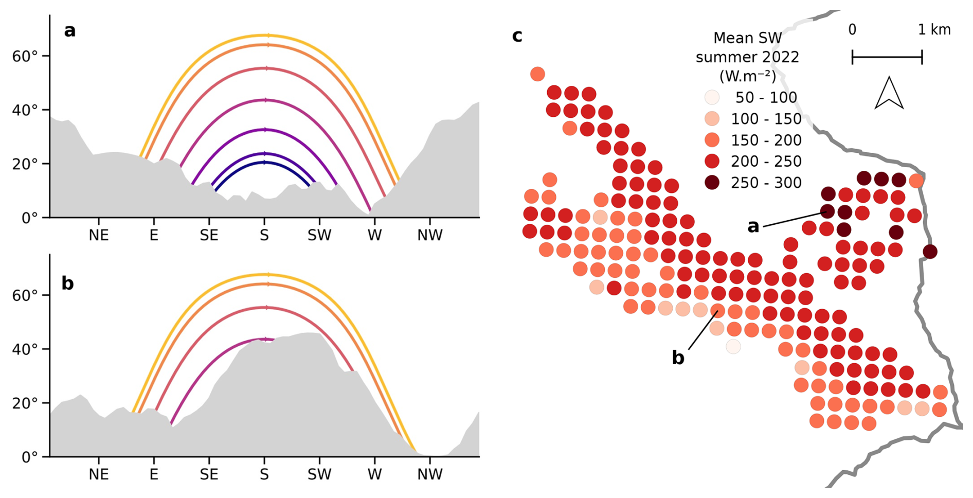
Figure C3 (a, b) Example of illumination masks at two locations over Argentière Glacier. Aspect resolution is 5°. The lines represent the sun trajectories (from top to bottom) on 21 June (yellow line), 21 May and 21 July, 21 April and 21 August, 21 March and 21 September, 21 February and 21 October, 21 January and 21 November, 21 December (blue line). (c) Mean shortwave radiation during summer 2022 (1 May to 30 September) from SAFRAN with illumination masks.

Appendix D: Evaluation extension

Figure D1 Extension of Fig. 3 with (a) dust simulations in orange (analogous to Fig. 3), and (b) no-dust simulations in blue.

Appendix E: Results extension

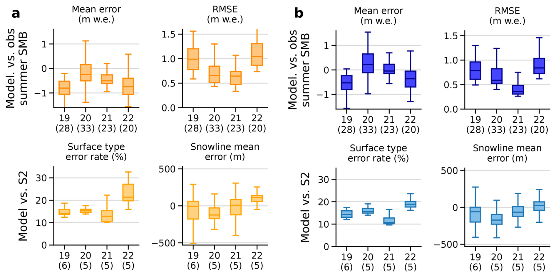
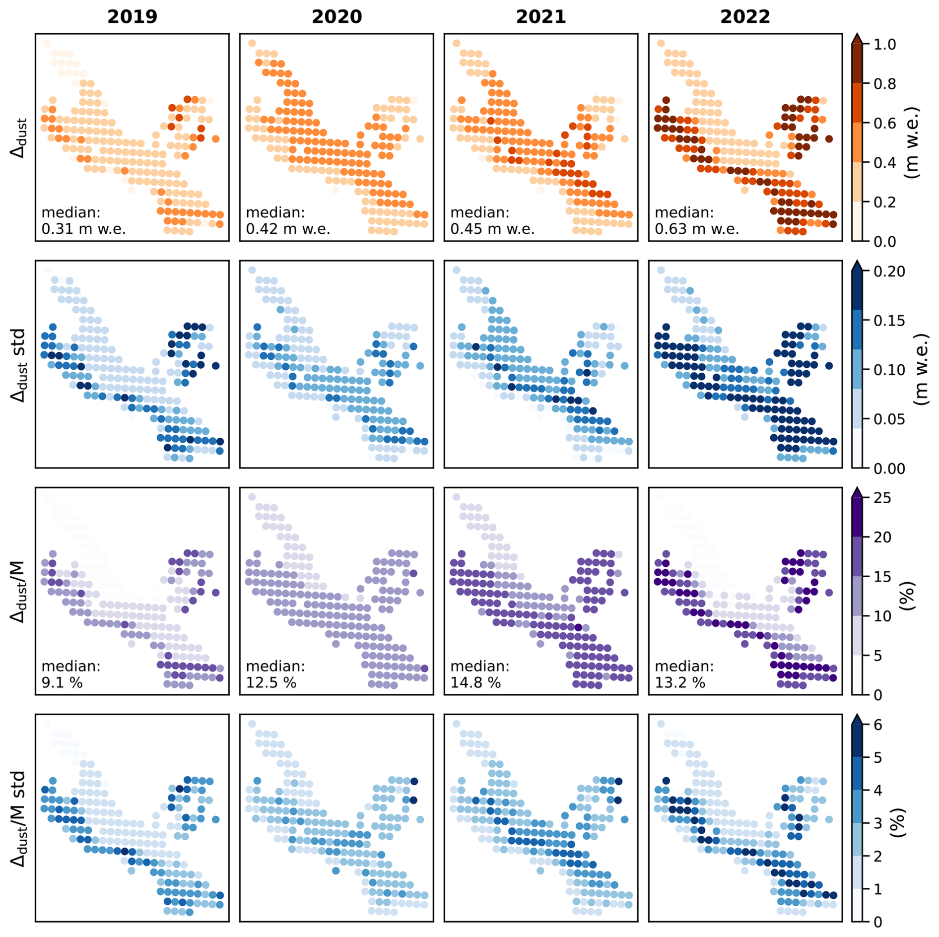
Figure E1 Extension of Fig. 6 for the years 2019 to 2022. Dust impact Δ_dust and melt fraction ${\mathrm{\Delta }}_{\text{dust}}/\text{M}$ with the associated standard deviation of the ensemble. The median of the ensemble is represented at each point. The aggregated value refers to the median (over the 40 members) of the mean over all simulation points.

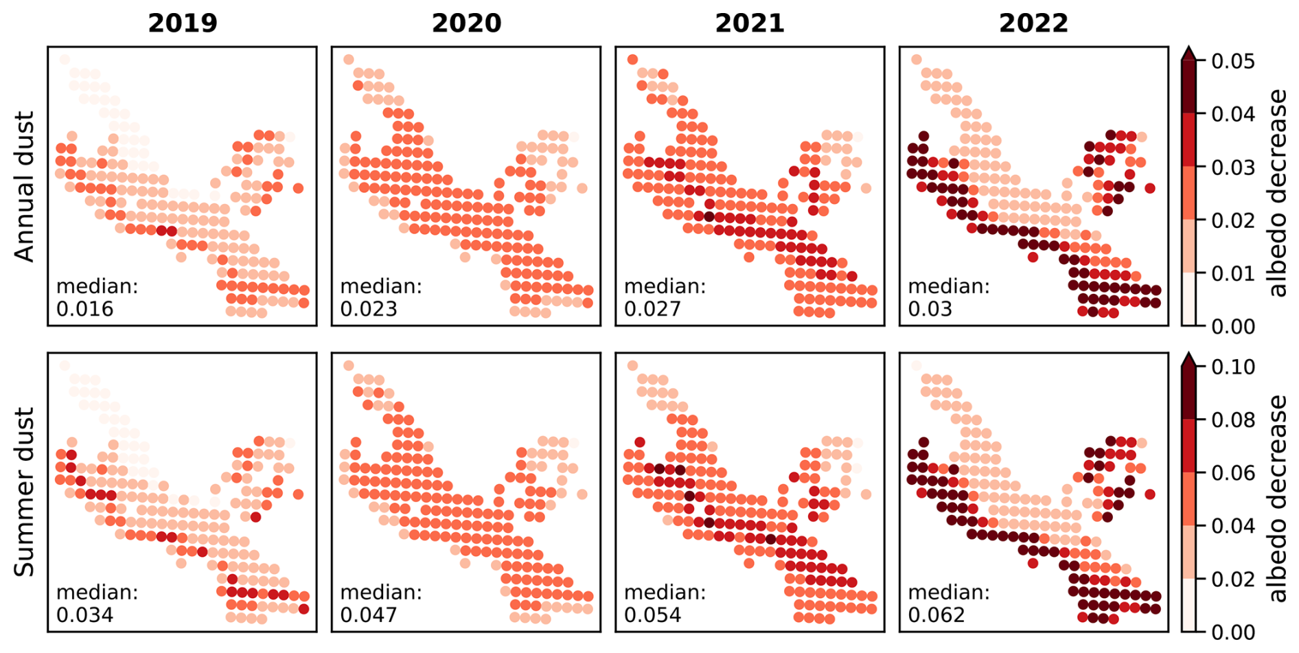
Figure E2 Extension of Fig. 6 for the years 2019 to 2022. Annual and summer albedo decrease due to dust. The median of the ensemble is represented at each point. The aggregated value refers to the median (over the 40 members) of the mean over all simulation points.

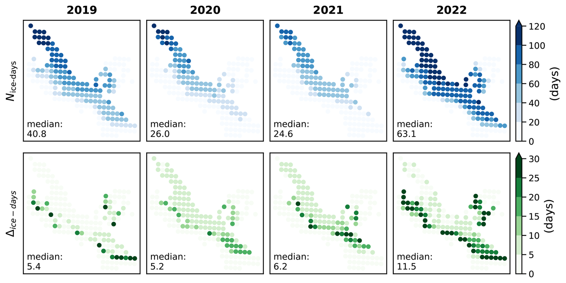
Figure E3 Extension of Fig. 6 for the years 2019 to 2022. Number of days with ice exposed at the surface for the dust simulation, and number of days with ice exposed for the dust simulation but not for the no-dust simulations. The median of the ensemble is represented at each point. The aggregated value refers to the median (over the 40 members) of the mean over all simulation points.