Air clathrate hydrates in the EDML ice core, Antarctica

In the deeper part of polar ice sheets, air hydrates trap most of the ancient air molecules, which are essential for understanding past climate. We use digital image analysis to create a high-resolution record of air hydrate number, size, and shape from ice thick-section microphotographs of the EPICA Dronning Maud Land (EDML) ice core, Antarctica, over a depth range from 1255–2771 m. We confirm that the air hydrate number and size correlate with paleoclimate and that the correlation disappears in the deeper parts of the ice core, which was previously shown for the Vostok and Dome Fuji ice cores in Antarctica and the GRIP ice core in Greenland. We also observe that the air hydrates grow with depth. Furthermore, we identify two peculiarities: a distinctive change in air hydrate aspect ratio (AR) and orientation at about 2030 m and a region of increased air hydrate clustering from 2392–2545 m depth. Remarkably, they coincide with regions of distinctive changes in ice microstructure as a response to changes in local ice dynamics; therefore, we discuss the influence of ice deformation on the air hydrate ensemble.

1 Introduction

Polar ice cores are a unique climate archive, as they provide the most direct record of past atmospheric greenhouse gas compositions (e.g., Raynaud et al., 1993). In the shallower parts of polar ice sheets, below the firn-to-ice transition, air bubbles are the main type of air inclusions. In the bubble-to-hydrate transition zone (BHTZ), air bubbles gradually transform to clathrate hydrates of air (hereinafter, air hydrates). Air hydrates are a guest–host compound with a crystalline framework of hydrogen-bonded water molecules forming cages (host) in which individual air molecules (guests) are trapped (e.g., Chazallon and Kuhs, 2002). X-ray diffraction studies on single crystals of air hydrates in the Dye-3 and Vostok ice cores revealed the Stackelberg's crystallographic structure II (sII; Hondoh et al., 1990; Takeya et al., 2000). At standard temperature and pressure, 1 volume of air hydrate can store up to 150 volumes of air (Uchida et al., 2011). Therefore, after the completion of the bubble-to-hydrate transformation, air hydrates are considered to trap most of the ancient air molecules in polar ice (Uchida et al., 2011). Extensive records of air hydrate number concentration (N_ah), size, and shape were acquired for the Vostok (Uchida et al., 1994a; Lipenkov, 2000) and Dome Fuji (Narita et al., 1999; Ohno et al., 2004; Uchida et al., 2011) ice cores in Antarctica and the GRIP ice core in Greenland (Pauer et al., 1999) using optical light microscopy. It was discovered in these investigations that the air hydrates' N_ah and mean size correlate with past climatic changes. Generally, ice formed during colder conditions is characterized by a higher N_ah of smaller air hydrates, while ice formed during warmer conditions has a lower N_ah of larger air hydrates (e.g., Uchida et al., 1994a; Pauer et al., 1999). It is suggested that this relation originates in the formation of air bubbles at the firn–ice transition, which is connected to the grain size of the ice matrix and therefore to the temperature and accumulation rate prevailing during the snow-to-ice transformation (Lipenkov, 2018, 2000; Lipenkov and Salamatin, 2014; Spencer et al., 2006). Higher temperatures and lower accumulation rates lead to bigger grains and, as a result, to bigger, but fewer, air bubbles. Despite the intricate processes that govern the conversion of air bubbles to air hydrates, the correlation between the number concentration and the size of air inclusions with different climatic conditions persists after the BHTZ (Uchida et al., 1994a; Lipenkov, 2000). With increasing depth, the air hydrate ensemble evolves due to physicochemical processes such as (a) fragmentation and recrystallization (Kipfstuhl et al., 2001) and (b) air molecule diffusion and subsequent crystal growth (e.g., Salamatin et al., 2003; Uchida et al., 2011) occurring within the ice sheet.

The EPICA Dronning Maud Land (EDML) deep ice core was drilled at Kohnen Station in East Antarctica (79°00^′ S, 0°04^′ E; elevation 2892 $\mathrm{m}\mathrm{a}.\mathrm{s}.\mathrm{l}.$) from the years 2001 to 2006. The maximum logging depth is 2774.15 m (Wilhelms et al., 2014), and the borehole inclination is roughly between ±3° (Weikusat et al., 2017). It differs from other Antarctic deep ice cores from the East Antarctic Plateau by a current higher accumulation rate (about 7 cm a⁻¹ ice equivalent) and higher annual average surface temperatures (−45 °C), which allowed paleoclimatic records to be obtained at a high temporal resolution (e.g., EPICA Community Members, 2006). It is dated down to about 2415 m depth, or 145 kyr (Ruth et al., 2007; Bouchet et al., 2023), and the BHTZ extends from 700 to 1225 m (Bendel et al., 2013). The ice cores' location on an ice divide and the possibility to analyze air hydrates' properties with a higher temporal resolution, compared to the Dome Fuji and Vostok ice cores, provide an interesting and novel case for the study of air hydrate inclusions.

Typically, the quantification of air hydrates and their properties in polar ice required tedious and time-consuming manual measurements: approximately 200 inclusions per sample were characterized to obtain statistically representative values. In the past years, digital optical microscopy and automatic image analysis were employed to characterize ice grains and grain boundary structures (Kipfstuhl et al., 2009; Binder et al., 2013) as well as air bubble inclusions (Ueltzhöffer et al., 2010; Bendel et al., 2013). Automated image analysis offers advantages compared to manual methods, such as repeatability and analysis speed, and allows the investigation of larger datasets.

In this work, for the first time, we apply traditional image analysis algorithms on ice thick-section microphotographs to analyze air hydrates in an ice core. Altogether, we measure and evaluate about 183 000 air hydrates in 110 000 images, which belong to 74 ice thick-section samples from the EDML ice core (Kipfstuhl, 2007). The aim of this contribution is to provide a high-resolution record of air hydrate properties below the BHTZ of the EDML ice core. We investigate the correlation of the air hydrate properties and past climate at higher resolution than previously possible for other Antarctic ice cores. In addition, we examine the air hydrate evolution via depth.

2 Data and methods

2.1 Dataset: EDML thick-section images

In the course of the EDML microstructure mapping project (Kipfstuhl et al., 2006; Kipfstuhl, 2007), microphotographs of vertical ice thick sections (∼ $\mathrm{90}\mathrm{mm}\times \mathrm{45}\mathrm{mm}\times \mathrm{4.5}\mathrm{mm}$) of the EDML ice core were acquired at every 10 m depth interval. For this study, we selected microphotographs of 74 thick sections in the depth range of 1255–2774 m, i.e., below the BHTZ at EDML. The images are unique because they were recorded during three Antarctic field seasons (2002–2006) within a few days after the sample was drilled. An exception is 10 microphotographs from 1314 to 1554 m, which were obtained 5 months after drilling. Air hydrates decompose during the long time storage of the ice samples (Uchida et al., 1994b); therefore, the imaging as soon as possible after core retrieval is crucial. The microstructure mapping setup consisted of an optical microscope (Leica DMLM), a CCD video camera (Hamamatsu C5405), a frame grabber, and a software-controlled xy stage (Kipfstuhl et al., 2006). Images were taken in transmission focusing on the surface and into the sample about one-third and two-thirds below the surface. Recording of one sample results in a mosaic image, which is composed of approximately 1500 individual images (tiles), each consisting of 768 pixel×512 pixel with a resolution of 3.25 µm per pixel. For this study, mosaic images located about 1.5 mm below the sample surface were analyzed. Sample preparation and image acquisition (microstructure mapping) are described in detail in Kipfstuhl et al. (2006).

2.2 Optical and imaging properties of air hydrates

Uchida et al. (1995) measured the mean refractive index of an air hydrate crystal in polar ice and determined it to be 1.3137 (±0.0016), which is slightly higher than the refractive index of ice (1.3084±0.0007). The higher refractive index of air hydrates was also confirmed by the Becke test (Shoji and Langway, 1982). Reflection and refraction at the ice–air hydrate boundary focus the light locally to form a bright rim (Becke line) and a corresponding shadow creating different “core” and “rim” appearances (A–F in Fig. 1). As a consequence, air hydrates appear in the images with varying optical characteristics, depending on the location to the focus plane. Hydrates close to the plane of perfect focus (or the depth of field) (A, C in Fig. 1) show a small “rim” and a “core” with a brightness close to the pure ice background. Hydrates above the focus plane are characterized by a distinctly darker “core” and a bright “rim” (E in Fig. 1), and hydrates below the focus plane are characterized by a brighter “core” and a darker “rim” (B, D in Fig. 1). Hydrates which are outside of the “hydrate-mapping depth” (F in Fig. 1) are hardly, or not at all, distinguishable from the ice background or image artifacts (III in Fig. 1). The presence of these hydrates can only be confirmed by comparing images of different focus levels of the same sample (cf. Sect. 2.1). Qualitatively, both the mean gray value of the hydrate's core and the thickness of the rim depend on the distance to the focus plane. Furthermore, other optical features, such as secondary formed air bubbles (I in Fig. 1), grain boundaries (II, IV in Fig. 1), and unidentifiable inclusions (V in Fig. 1), are present in the images as artifacts.

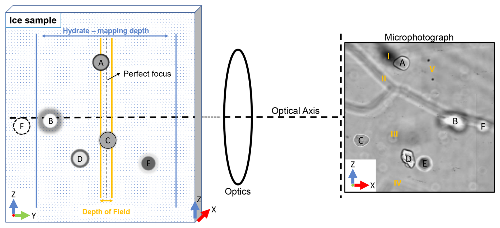
Figure 1 This figure (“horizontal microscope”) shows the different visual categories (A–F) of air hydrates present in the image dataset, which depend on their relation to the focus plane and on other optical features (I–V). The Z axis is parallel to the core axis and points towards the “top” direction.

2.3 Image processing

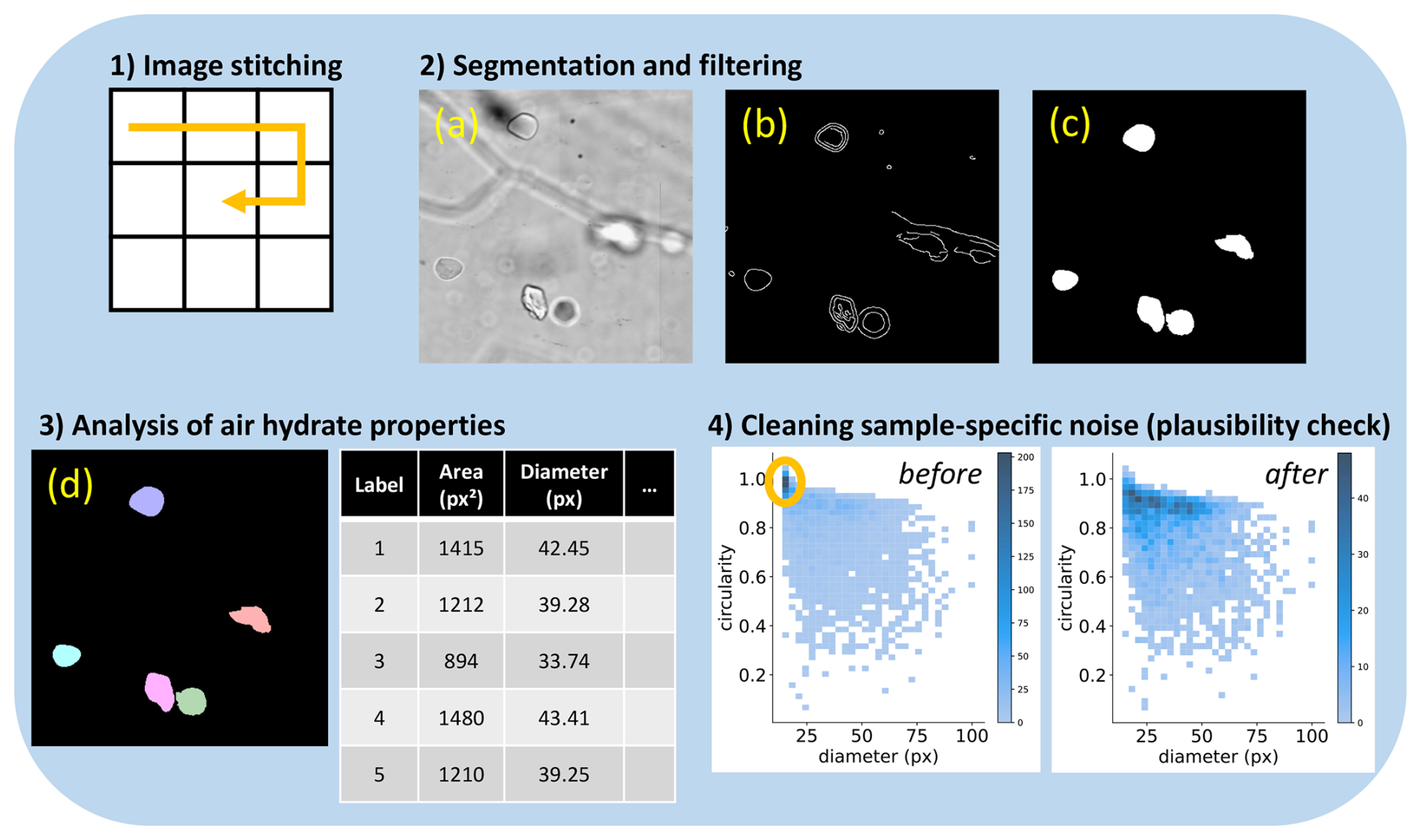
Python 3 (version 3.10.13) and the open-source libraries NumPy (2.1.3), scikit-image (0.24.0), scikit-learn (1.5.2), and Pandas (2.2.3) are utilized for the image- and data-processing workflows. The routines were implemented on an HP EliteBook 850 G8 with an Intel Core-i5 CPU and 32GB physical memory. The image data can be processed and analyzed within 1 d. Our image-processing and analysis workflow consists of four steps: (1) image stitching, (2) segmentation and filtering, (3) connected component analysis, and (4) a plausibility check (Fig. 2).

Figure 2 Image-processing and analysis workflow.

2.3.1 Image stitching

We used a semi-automatic stitching script and fixed offset parameters to merge the 1500 individual tiles into a single mosaic image in a “snake-by-rows” way (Fig. 2). The optimal offset parameters for each of the 74 mosaic images were determined manually. To remove artifacts at the sample edges, the mosaic images were cropped into 80 mm×30 mm. Then, they were manually sorted into six different categories depending on acquisition time (i.e., field season), brightness, and contrast conditions for further image segmentation (Fig. A1).

2.3.2 Air hydrate segmentation and filtering

Segmentation separates regions with specific characteristics within an image from a background (e.g., air hydrates from an ice background). Objects and background in an image are divided by edges, which are rapid local changes in image color, intensity, or texture (Jing et al., 2022; Szeliski, 2022). We use the Canny edge detection algorithm (Canny, 1986), which is one of the most popular edge detection methods (Jing et al., 2022), to produce a binary edge map (Fig. 2b). Then, we apply a combination of binary morphological operators (i.e., dilation and erosion) and selective filtering to obtain the final segmentation result, where air hydrates correspond to white pixels and the background corresponds to black pixels (Fig. 2c). The individual steps of the segmentation routine are described in detail in Appendix B1. Due to different imaging conditions (i.e., contrast and brightness), which were caused by, among other things, the image acquisition during different Antarctic field seasons, the performance of the edge detection algorithm may vary. Accordingly, we slightly adjusted the segmentation parameters to each of the six image categories by optimizing the segmentation metrics for several manually segmented images, hereinafter ground truth (GT) images (see Sect. 2.4 for details).

2.3.3 Analysis of air hydrate properties

In the final segmented image, each object is assigned a unique label and henceforth considered to be one air hydrate (Fig. 2d). Analyzed pristine properties include the area (i.e., number of pixels =A_ah), perimeter, and mean gray value from which further parameters were calculated (see Eqs. 1–3). We defined the size of each air hydrate as the equivalent diameter (D) of a circle having the same A_ah as the object's projection.

$$\begin{array}{}\text{(1)}& {\displaystyle }{\displaystyle }D=\mathrm{2}\cdot \sqrt{{\displaystyle \frac{A_{\text{ah}}}{\mathit{\pi }}}}\end{array}$$

The volume (V) of an air hydrate is estimated using a spherical approximation.

$$\begin{array}{}\text{(2)}& {\displaystyle }{\displaystyle }V={\displaystyle \frac{\mathit{\pi }(D{)}^{\mathrm{3}}}{\mathrm{6}}}\end{array}$$

The circularity is a measure of the similarity of an object to a circle, where 1 denotes a perfect circle and 0 denotes a highly non-circular shape:

$$\begin{array}{}\text{(3)}& {\displaystyle }{\displaystyle }\text{circularity }={\displaystyle \frac{\mathrm{4}\mathit{\pi }\cdot A_{\text{ah}}}{{\text{perimeter}}^{\mathrm{2}}}}.\end{array}$$

In order to analyze the aspect ratio (AR) and orientation, we fitted an ellipse to each air hydrate using scikit-image (van der Walt et al., 2014). We defined the air hydrates' AR as the ratio of the major to the minor axis of the fitted ellipse and the orientation as the angle (α) between the semi-major axis and the x axis of the microphotographs. The measured values for α range from 90 to −90° (≡ N to S on a compass), where 0° represents a preferred elongation parallel to the image x axis or, in other words, normal to the core axis (geographic horizontal). For the evaluation of the orientation data, we considered only those air hydrates whose ratio of major to minor axis is higher than 4:3 (i.e., an AR higher than 1.33).

2.3.4 Cleaning sample-specific noise (plausibility check)

We examined two-dimensional histograms of the diameter against circularity (Fig. 2), AR, and mean gray value for each air hydrate in a sample in order to perform a plausibility check of the segmentation. This method allows a fast visual assessment by inspecting and comparing the resulting patterns of the 2D histograms. For samples from 1314, 2055, and 2115 m depth, an additional filter, based on the results of the plausibility check, was applied to remove sample-specific noise. For instance, for the sample from 1314 m, small and round (small diameter and high circularity) objects were removed from the dataset (Fig. 2).

2.4 Segmentation evaluation and metrics

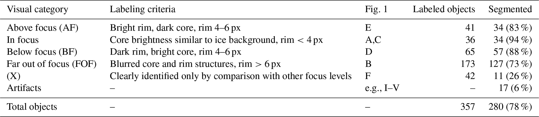
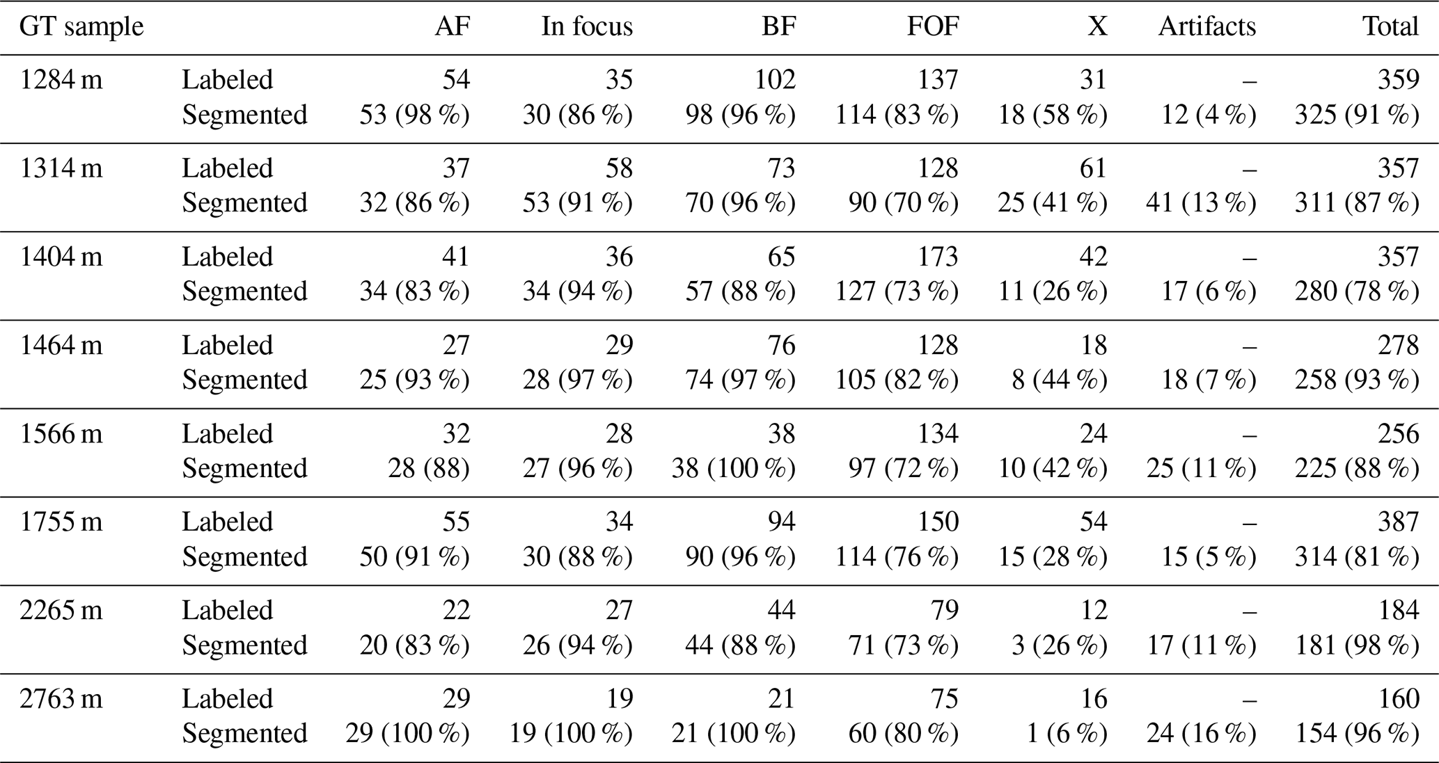
To evaluate the segmentation routine, we created eight ground truth (GT) images with dimensions of 20 mm×10 mm. They were selected to represent the six image categories and to reflect the diversity of the dataset (Fig. A1). Each GT image contains 160–387 air hydrates which were traced by hand and classified into five visual categories using the ImageJ/Fiji plugin LABKIT (Arzt et al., 2022). Emphasis was placed on labeling an image in one run and the individual images in quick succession in order to keep human bias as low as possible. The labeling criteria, an example distribution, and a segmentation performance of each visual category can be seen in Table 1. Note that, although the output of the segmentation routine produces a binary image (two classes: air hydrates and background), the introduction of the five hydrate categories in the GT image is useful for a deeper understanding of the performance of each routine and the raw image data.

Table 1 Air hydrate visual categories and their segmentation probability for the GT image of the sample from 1404 m depth.

2.4.1 Evaluation of individual air hydrates

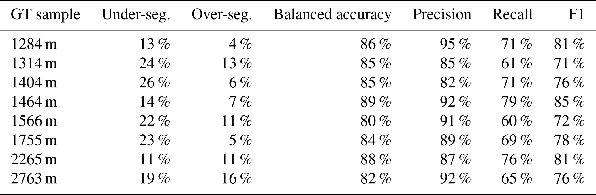
To determine the number of detected air hydrates for each category (cf. Table 1), each air hydrate, together with its bounding box enlarged by 12 pixels, was cut out from the GT image and automatically compared with the corresponding cutout in the segmented image. The air hydrate was detected if pixels in the cutouts overlap, while an “empty” cutout of the segmented image, or the lack of overlapping pixels, implies that the air hydrate was not detected. We then calculated the percentage of under-segmentation, i.e., the proportion of unrecognized hydrates, and the percentage of over-segmentation, i.e., the proportion of erroneously segmented objects (cf. Table 2). The data for all GT images are shown in Table B1 and were additionally verified by visual inspection.

Table 2 Segmentation metrics for the eight GT images.

To determine the size discrepancy between GT and segmented air hydrates, we compared the air hydrates' sizes in the abovementioned cutouts. Figure 3 shows the stacked distribution of differences in diameter between the GT and segmented air hydrates in percent (%). We defined the measurement error of the air hydrate diameter as the standard deviation of this distribution considering the negative skew ($-\mathrm{26}\mathrm{\%}/+\mathrm{14}\mathrm{\%}$). Air hydrates which are far out of focus (e.g., B in Fig. 1) cause the negative skewed distribution and are the main component of this error (Fig. 3). Note that the manual tracing of air hydrates far out of focus should be regarded as a “best estimate” due to the blurred core and rim structures. In conclusion, the true size will be preferentially underestimated.

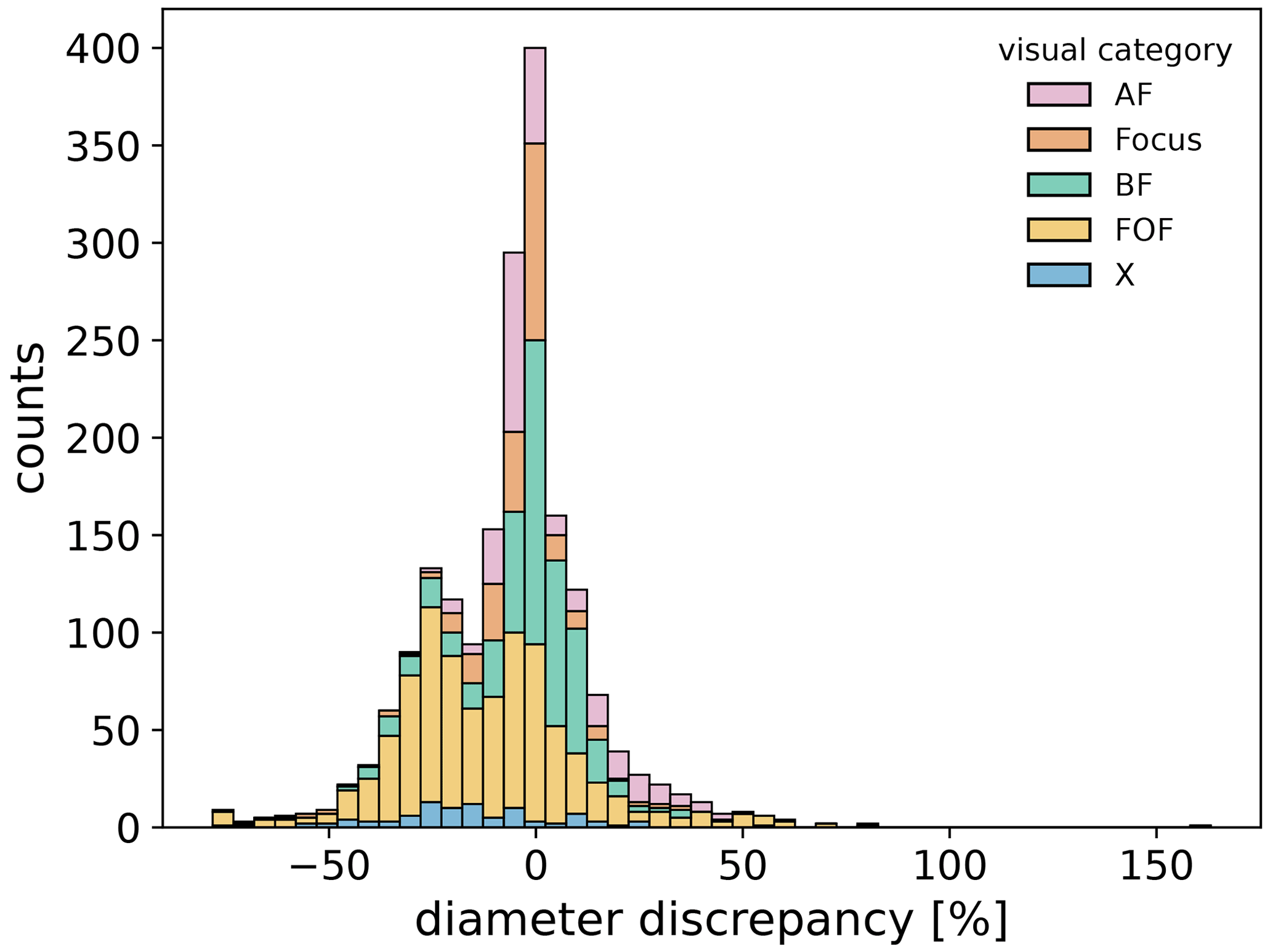
Figure 3 Stacked distribution of diameter discrepancy for each air hydrate in the eight GT images compared to the corresponding segmented image. The different colors and abbreviations correspond to the different visual categories in Table 1. The mean value and standard deviation are −6 % and ±20 %, respectively.

2.4.2 Evaluation of general segmentation quality

To evaluate the general segmentation quality, we compared the GT images pixel by pixel with the segmented images. Each pixel in the segmented image can adopt one of four properties: (1) true positive (TP), where the pixel is correctly segmented as air hydrate; (2) false positive (FP), where the pixel is incorrectly segmented as air hydrate; (3) true negative (TN), where the pixel is correctly segmented as background; and (4) false negative (FN), where the pixel is incorrectly segmented as background. These values are then the basis for calculating specific metrics to determine the quality of the segmentation routine (see Eqs. 4–7).

The accuracy score shows the proportion of pixels correctly segmented, among all the pixels in the image. This metric can be biased if there is an imbalance in classes, e.g., background pixels and air hydrate pixels. Therefore, we use the balanced accuracy score defined as the average accuracy obtained on either class (Brodersen et al., 2010):

$$\begin{array}{ll}{\displaystyle }\text{balanced accuracy}=& {\displaystyle \frac{\mathrm{1}}{\mathrm{2}}}\left({\displaystyle \frac{\text{TP}}{\text{TP}+\text{FN}}}+{\displaystyle \frac{\text{TN}}{\text{TN}+\text{FP}}}\right)\\ \text{(4)}& {\displaystyle }& {\displaystyle }\cdot \mathrm{100}\mathrm{\%}.\end{array}$$

The precision metric is the proportion of pixels actually labeled as air hydrates among all the pixels segmented as air hydrates:

$$\begin{array}{}\text{(5)}& {\displaystyle }{\displaystyle }\text{precision}={\displaystyle \frac{\text{TP}}{\text{TP}+\text{FP}}}\cdot \mathrm{100}\mathrm{\%}.\end{array}$$

Recall is defined as the proportion of pixels correctly segmented as air hydrates among all the pixels that are labeled air hydrate pixels:

$$\begin{array}{}\text{(6)}& {\displaystyle }{\displaystyle }\text{recall}={\displaystyle \frac{\text{TP}}{\text{TP}+\text{FN}}}\cdot \mathrm{100}\mathrm{\%}.\end{array}$$

The F1 score calculates the harmonic mean between precision and recall and balances the error contribution of false negatives and false positives:

$$\begin{array}{}\text{(7)}& {\displaystyle }{\displaystyle }\text{F1}={\displaystyle \frac{\mathrm{2}\text{TP}}{\mathrm{2}\text{TP}+\text{FP}+\text{FN}}}\cdot \mathrm{100}\mathrm{\%}.\end{array}$$

We determined the pixelwise segmentation metrics (see Table 2) to optimize the segmentation routine (Sect. 2.3.2) and to allow a possible performance comparison with future segmentation methods.

2.5 Further considerations for data interpretation

2.5.1 Convert air hydrate counts to air hydrate number concentration

We convert the measured air hydrate counts per sample to N_ah using the measured ice-sample thickness (mean value of six consecutive measurements, typically 4.53±0.49 mm) and the cropped mosaic image dimensions (80 mm×30 mm). Air hydrate counts per sample and N_ah have a good linear correlation (Fig. 4), and we conclude that the observed volume (i.e., hydrate-mapping depth; Fig. 1) is consistent for all samples. An exception could be the samples from 1255–1294 m (star markers in Fig. 4).

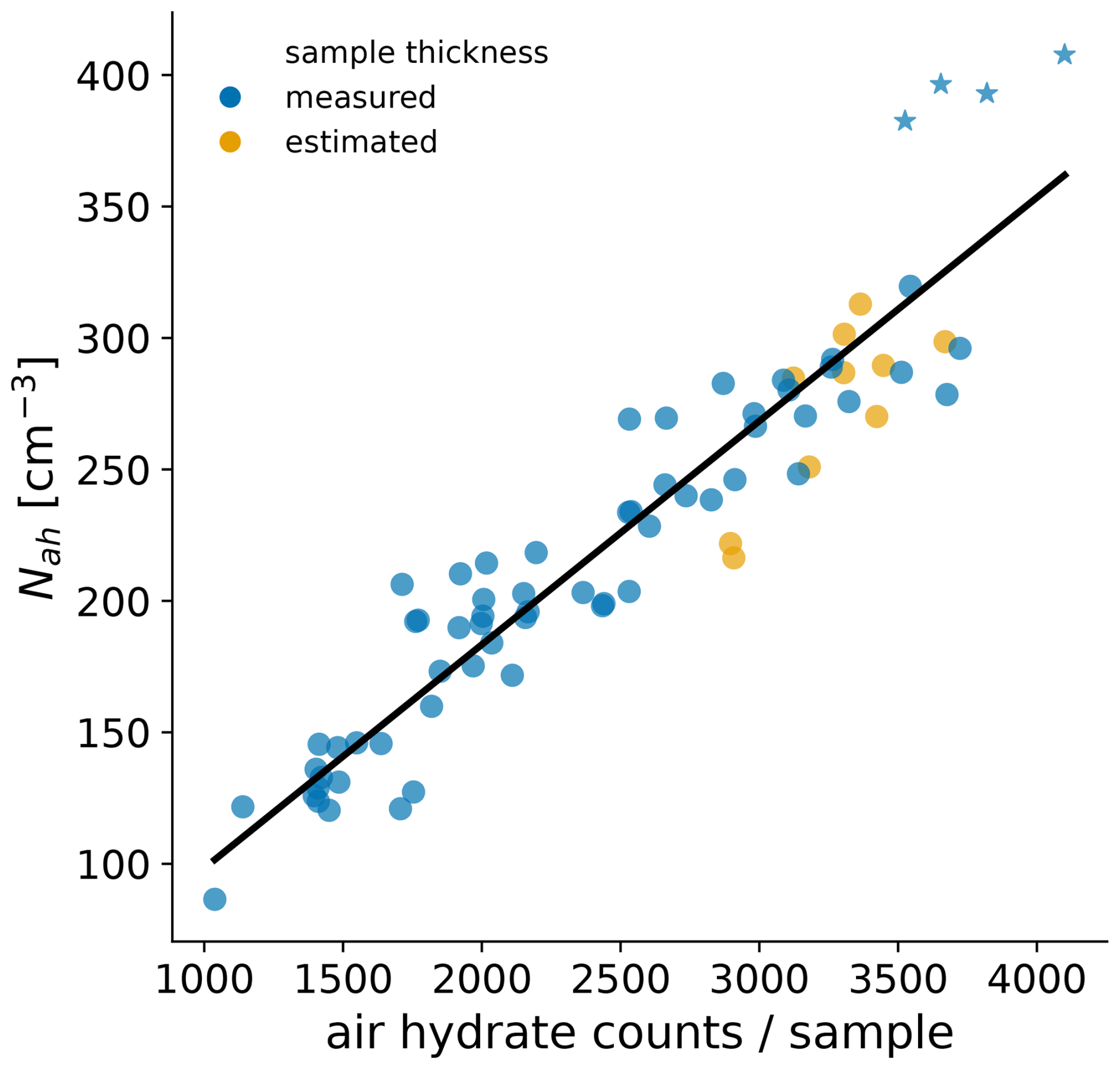
Figure 4 Air hydrate counts per sample plotted against number concentration ($R=-\mathrm{0.94}$, p<0.001). For samples from 1314 m to 1554 m, the sample thickness was estimated by the number of turns of the microscope's fine drive. Star markers correspond to samples from 1255–1294 m depth.

2.5.2 Influence of ice core rotation

An ice core is usually drilled in increments of 3–4 m. To preserve the orientation between two increments, they are manually fit together at the breakpoints during ice core logging (Hvidberg et al., 2002). Air hydrates in ice are translucent 3D objects which are projected to the image plane. Therefore, a loss of ice core orientation (i.e., rotation) could influence the analyzed shape characteristics of air hydrates. A detailed discussion can be found in Appendix C.

3 Results

3.1 Air hydrate number concentration and size

The main results, together with the stable water isotope (${{\mathit{\delta }}^{\mathrm{18}}\mathrm{O}}_{\text{ice}}$) record (EPICA Community Members, 2010; Oerter et al., 2025), a proxy for past climate and particularly past temperature, and the ice crystal grain size (Weikusat et al., 2009), are presented in Fig. 5. N_ah decreases from about 400 cm⁻³ at 1255 m to about 120 cm⁻³ at 2771 m, with fluctuations that broadly match the δ¹⁸O signal (Fig. 5a and b). The lowest N_ah of the record is 90 cm⁻³ and occurs at 2741 m. We measure an average N_ah of 290 cm⁻³ during the cold periods of MIS 4 and MIS 6, which is higher than the N_ah during the warmer Eemian (MIS 5e), where the average value is 190 cm⁻³. Surprisingly, no air hydrates were found in the lowermost sample at 2773.91 m depth. The sizes of the air hydrates in all samples, except possibly at 2545 and 2741 m depth, follow a log-normal distribution. Consequently, we determined the arithmetic mean diameter ($\stackrel{\mathrm{‾}}{D}$) and standard deviation (σ) by fitting a log-normal function. The values for the air hydrate mean diameter range from 110 to 176 µm (Fig. 5c). Generally, air hydrates are smaller during colder periods, with a mean value of 113 µm for MIS 4, and bigger during warmer periods, with a mean value of 140 µm for MIS 5e. Close to the bottom of the ice core, the mean diameter increases to a maximum of 176 µm. The width of the air hydrate size distributions, given here as the relative standard deviations (RSDs; $\mathit{\sigma }/\stackrel{\mathrm{‾}}{D}$), range from 33 % to 48 % (Fig. 5c). These values are nearly identical to those measured in the Vostok (Lipenkov, 2000) and Dome Fuji (Uchida et al., 2011) ice cores. From 1255 to 1635 m depth, the average RSD is 40 %, and, from 1635 m, it decreases to an average of 37 %. An exception is samples from ca. 1995 to 2115 m depth, where the RSD increases with a maximum of 43 % at ca. 2040 m. Furthermore, at the Eemian–MIS 6 transition, the RSD increases from 37 % to 43 %. Naturally, N_ah and mean diameter show a strong negative linear correlation (Fig. 6a); however, 10 anomalies (triangular markers) can be found for samples from 2382–2545 m depth (excluding the sample at 2385 m), where either N_ah or $\stackrel{\mathrm{‾}}{D}$ is overestimated. These samples correspond to “region 2” in the following figures and will be discussed in more detail below.

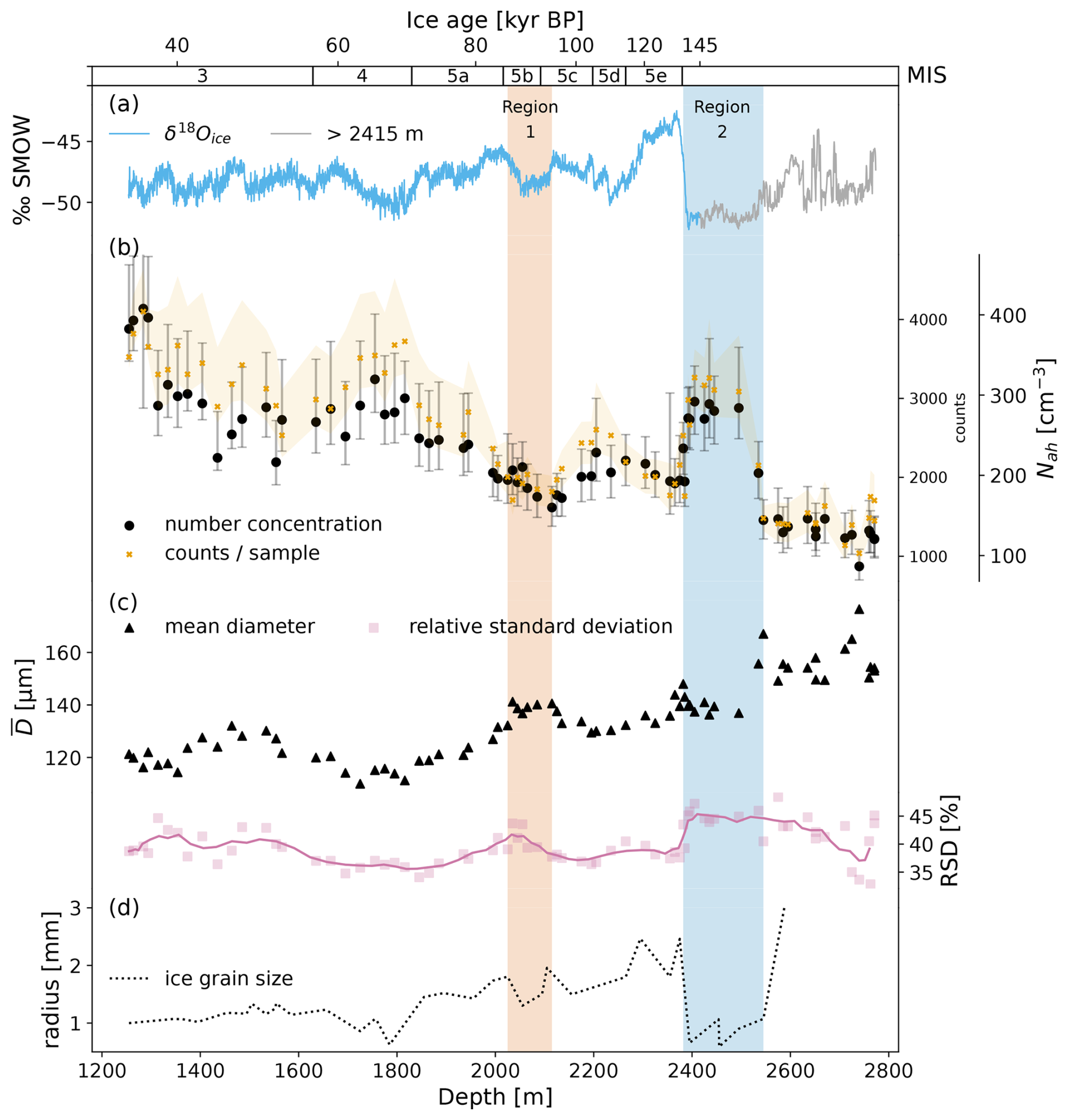
Figure 5 Air hydrate depth profiles of the EDML ice core. (a) Paleoclimatic information as ${{\mathit{\delta }}^{\mathrm{18}}\mathrm{O}}_{\text{ice}}$ values. Blue corresponds to the dated part of the ice core (EPICA Community Members, 2010), and gray corresponds to the non-dated part of the ice core (Oerter et al., 2025). (b) Air hydrate counts and number concentration (N_ah). The error band for air hydrate counts is explained in Sect. 2.4 and Table 2, and error bars are calculated including the uncertainty in sample thickness measurements. (c) Mean diameter ($\stackrel{\mathrm{‾}}{D}$) and relative standard deviation (RSD) and (d) ice grain size (Weikusat et al., 2009). The ice age at the top of the figure corresponds to the AICC 2023 for EDML (Bouchet et al., 2023). The MIS boundaries are defined by Lisiecki and Raymo (2005), and the MIS 5 substage boundaries are from Otvos (2015). Shaded bands correspond to “region 1” and “region 2” discussed in the text (especially in Sect. 4.2.1 and 4.2.2).

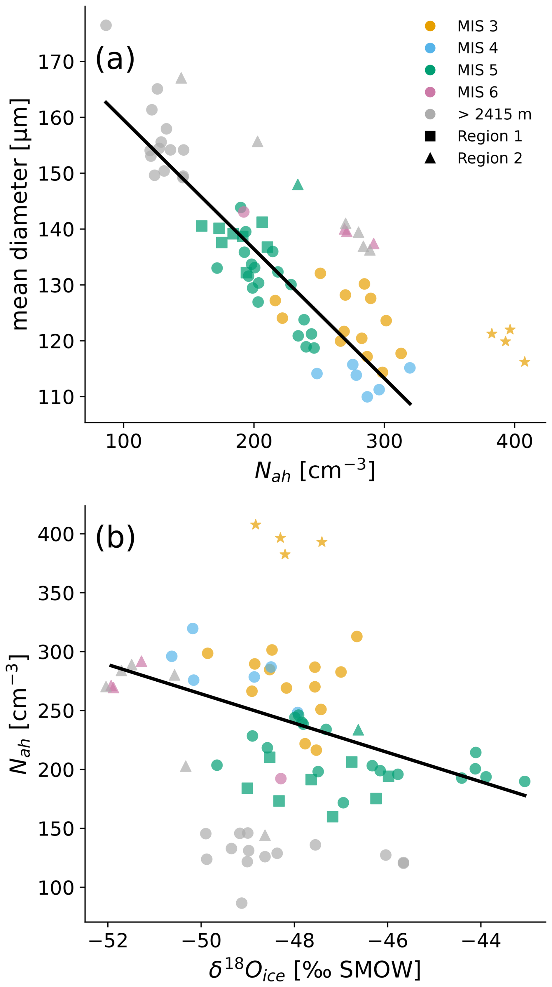
Figure 6 (a) N_ah plotted against $\stackrel{\mathrm{‾}}{D}$. The linear correlation and the Pearson correlation coefficient are calculated without considering data from 1255–1294 m (star markers) and region 2 ($R=-$0.92, p<0.001). (b) ${{\mathit{\delta }}^{\mathrm{18}}\mathrm{O}}_{\text{ice}}$ plotted against N_ah. The linear correlation and the Pearson correlation coefficient are calculated without considering samples from 1255–1294 m and deeper than 2415 m ($R=-\mathrm{0.57}$, p<0.001). Square markers correspond to samples from 2025–2115 m depth (region 1 in Figs. 5 and 8). Triangular markers correspond to samples from 2382–2545 m depth (region 2 in Figs. 5 and 8).

Overall, the depth profiles of air hydrate number concentration and mean diameter show a trend of decreasing N_ah and increasing $\stackrel{\mathrm{‾}}{D}$ with increasing depth and thus increasing age, and they practically co-vary with the δ¹⁸O signal (Fig. 5a–c).

3.1.1 Comparison of air hydrate number concentration with air bubble concentration at EDML

Assuming a 1:1 conversion ratio between air bubbles and air hydrates, we estimate the detection rate of our method by comparing our measured N_ah with N_ab at EDML. Bendel et al. (2013) report an air bubble number concentration (N_ab) of 300–400 cm⁻³ for Holocene ice and 400–500 cm⁻³ for ice formed during the Last Glacial Maximum (LGM). Note that LGM ice at EDML is located within the BHTZ (at about 1000 m depth); therefore, air bubbles are already converting to air hydrates. Lipenkov (2018) describe a semi-empirical model relating air bubble number and sizes to climate parameters and ice formation conditions (firn temperature, accumulation rate, and surface snow density). Using this model, we estimate N_ab for present-day conditions at EDML (−44.5 °C, 6.4 $\mathrm{g}{\mathrm{cm}}^{-\mathrm{2}}{\mathrm{yr}}^{-\mathrm{1}}$, 0.38 g cm⁻³) to be about 400 cm⁻³ and N_ab in the LGM ice (assuming −54 °C, 3 $\mathrm{g}{\mathrm{cm}}^{-\mathrm{2}}{\mathrm{yr}}^{-\mathrm{1}}$, 0.38 g cm⁻³) to be about 475 cm⁻³. We then compare our measured N_ah for MIS 5e, as an analog for Holocene conditions, and compare MIS 6, to represent the LGM, with N_ab. As a result, we detect between 48 %–63 % of the expected N_ah. One explanation could be that the hydrate-mapping depth in our microscopic setup might not correspond to the physical sample thickness (Fig. 1). In other words, microphotographs from one focus plane might not display the entire sample volume.

3.2 Air hydrate mean volume, volume concentration, and air content

Figure 7 shows the mean volume (V_m) and volume concentration (V_c) of air hydrates and the theoretical total air content included in the air hydrate crystals (TAC_h). We estimated the average volume of an air hydrate (V_m) using the arithmetic mean of the volumes of all air hydrates included in a sample. V_m is increasing with depth from about $\mathrm{1.3}\times {\mathrm{10}}^{-\mathrm{6}}$ to about $\mathrm{3.0}\times {\mathrm{10}}^{-\mathrm{6}}$ cm³ (Fig. 7a). The volume concentration is defined as

$$\begin{array}{}\text{(8)}& {\displaystyle }{\displaystyle }{V}_{\mathrm{c}}=V_{\mathrm{m}}\cdot N_{\text{ah}}\end{array}$$

and is shown in Fig. 7b. It decreases from $\mathrm{5.0}\times {\mathrm{10}}^{-\mathrm{4}}$ at 1255 m to $\mathrm{3.0}\times {\mathrm{10}}^{-\mathrm{4}}$ at about 1700 m. Then, V_c stays relatively constant at about $\mathrm{3.4}\times {\mathrm{10}}^{-\mathrm{4}}$. A pronounced exception is observed for samples in the depth region from 2382–2545 m, where the V_c increases to an average of $\mathrm{5.7}\times {\mathrm{10}}^{-\mathrm{4}}$.

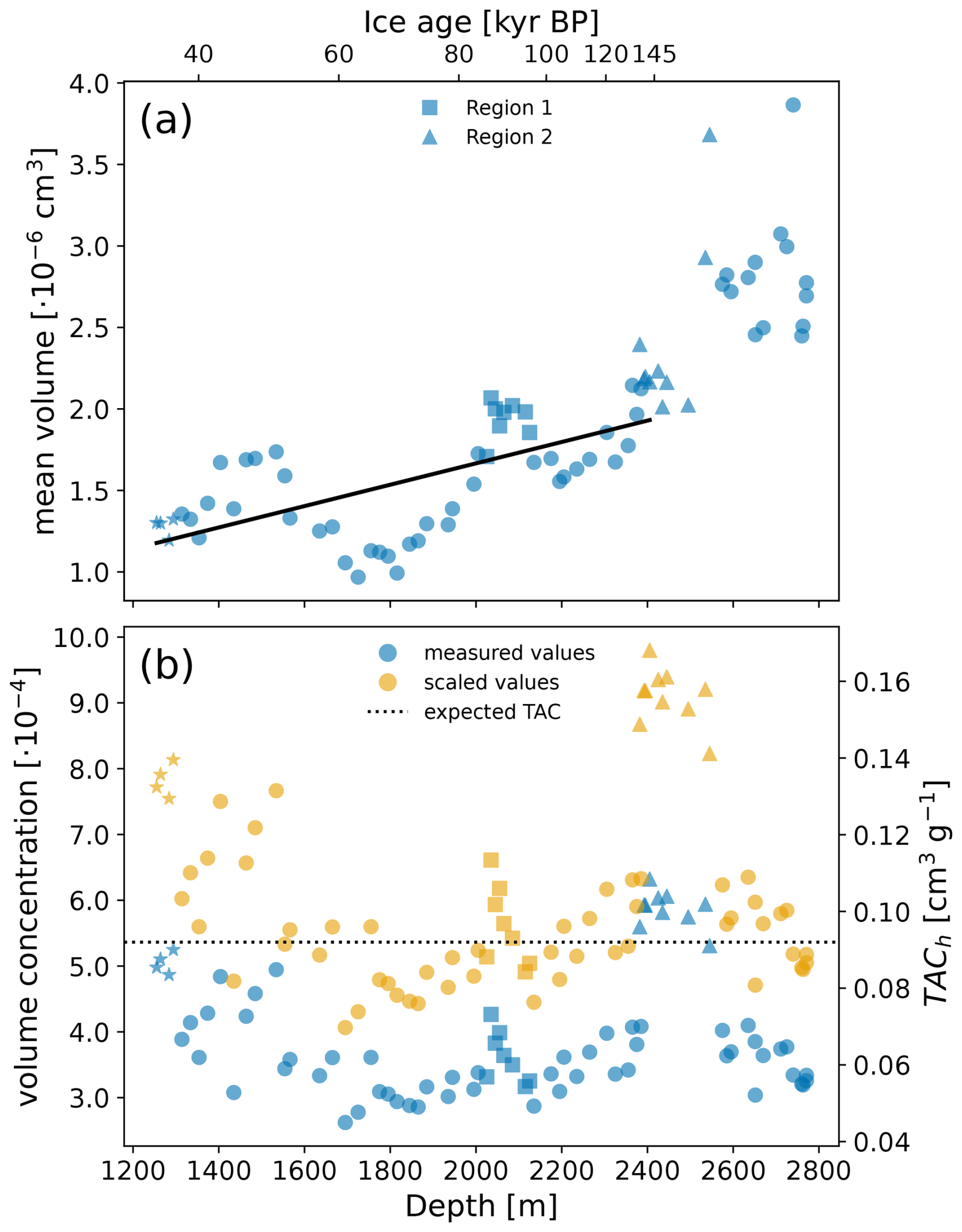
Figure 7 (a) Air hydrate mean volume. The solid line represents the calculated growth rate for the dated part of the EDML ice core (1255–2415 m; Ruth et al., 2007). (b) Blue markers: air hydrate volume concentration and total air content calculated from theoretical air content of air hydrates. Orange markers: scaled values to match expected mean TAC for EDML (dotted line at 0.092 cm³ g⁻¹; Martinerie et al., 1992). Star markers correspond to samples from 1255–1294 m depth. Square markers correspond to samples from 2025–2115 m depth (region 1 in Figs. 5 and 8). Triangular markers correspond to samples from 2382–2545 m depth (region 2 in Figs. 5 and 8). The ice age at the top of the figure corresponds to the AICC 2023 for EDML (Bouchet et al., 2023).

Using the air hydrates' crystallographic parameters, we estimated the TAC_h (Fig. 7b) at standard pressure and temperature following Lipenkov (2000):

$$\begin{array}{}\text{(9)}& {\displaystyle }{\displaystyle }{\text{TAC}}_{\mathrm{h}}={\displaystyle \frac{n\mathit{\alpha }}{a^{\mathrm{3}}{N}_{\mathrm{L}}}}\cdot {\displaystyle \frac{V_{\mathrm{c}}}{\mathit{\rho }}}.\end{array}$$

In the above equation, a is the air hydrate lattice constant ($\mathrm{1.72}\times {\mathrm{10}}^{-\mathrm{7}}$ cm), n is the number of cages per unit cell (24), and α is the cage occupancy (0.9; Lipenkov, 2000; Takeya et al., 2000). N_L is the Loschmidt constant (2.69×10¹⁹ cm⁻³), and ρ corresponds to the density of pure ice (0.92 g cm⁻³). Naturally, the TAC_h and V_c signals show the same pattern (Fig. 7b). The TAC_h decreases from 0.085 cm³ g⁻¹ at 1255 m to an average of 0.059 cm³ g⁻¹ from 1700 m down to the bottom of the ice core. From 2382–2545 m, the average TAC_h is 0.098 cm³ g⁻¹.

3.2.1 Comparison of TAC_h with total air content at EDML

The total air content (TAC) in polar ice is considered to depend on air pressure, temperature, and the pore volume in the firn at the time of pore close-off (e.g., Martinerie et al., 1992). As air hydrates contain most of the ancient air molecules in polar ice (Uchida et al., 2011), we can compare the calculated TAC_h with other independent TAC estimates. For EDML, a mean TAC of 0.0815 cm³ g⁻¹ was measured by a method integrated to a continuous flow analysis system (Ruth et al., 2004). This average value is lower than the TAC measured with absolute methods in Holocene ice cores from higher elevated drilling sites in Antarctica (Vostok, EDC; Martinerie et al., 1992). Therefore, we compare the calculated TAC_h to the theoretical TAC expected at EDML for an elevation of 2892 m a.s.l. and an atmospheric pressure of 650–700 mbar (about 0.092 cm³ g⁻¹) following Martinerie et al. (1992). The average TAC_h from 1700 m down to the bottom is 0.059 cm³ g⁻¹. This is about 64 % of the expected TAC and matches well with our estimations comparing N_ab and N_ah. Employing a scaling factor for the N_ah of 1.55, the average TAC_h for this depth region matches the expected TAC value (orange markers in Fig. 7b). Note that this scaling was not applied for the graphs and the data interpretation.

The high TAC_h values for the depth range from 1255–1700 m will be discussed in Sect. 4.1.1. The high TAC_h values for the depth range from 2382–2545 m (region 2) will be discussed in Sect. 4.1.2 and 4.2.2.

3.3 Air hydrate shape characteristics

The results of the air hydrate shape analysis, together with the ${{\mathit{\delta }}^{\mathrm{18}}\mathrm{O}}_{\text{ice}}$ record, the measured borehole temperature (Weikusat et al., 2017), and the second eigenvalue of the orientation tensor of the ice crystals' c-axis distribution (Weikusat et al., 2013), are presented in Fig. 8. The air hydrates' median aspect ratio decreases with depth, which means they become rounder (Fig. 8b). From 1255–2005 m, the AR is relatively constant with an average of 1.40; however, between 2005–2035 m, we observe a distinctive increase. From 2035–2395 m, the average AR is 1.50, with outliers at 2115, 2125, 2205, and 2305 m. From 2405 m down to the bottom, the AR decreases to an average value of 1.30. For every sample in the dataset, 90 % of measured air hydrates have an AR between 2.6–1.7 or smaller (Fig. 8c).

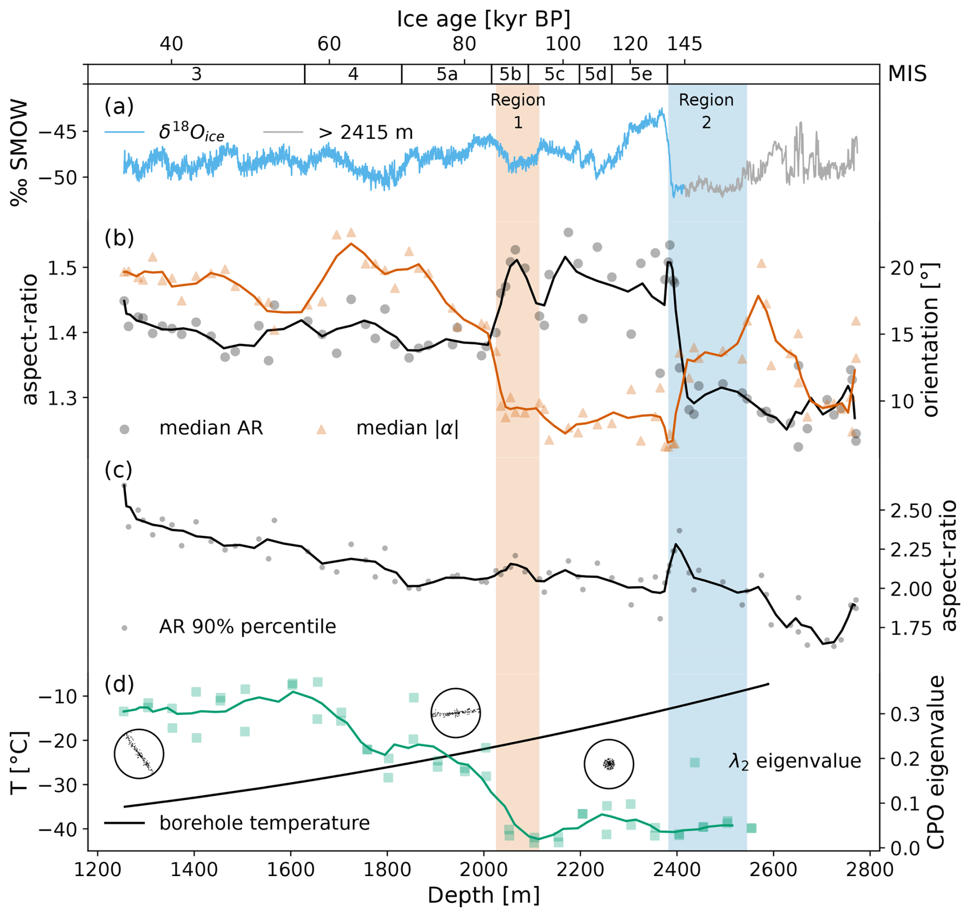
Figure 8 Shape characteristics of air hydrates in the EDML ice core. (a) Paleoclimatic information as ${{\mathit{\delta }}^{\mathrm{18}}\mathrm{O}}_{\text{ice}}$ values. Blue corresponds to the dated part of the ice core (EPICA Community Members, 2010), and gray corresponds to the non-dated part of the ice core (Oerter et al., 2025). (b) Air hydrate median AR and median of the absolute orientations ($\left|\mathit{\alpha }\right|$), (c) 90 % percentile of air hydrate AR, and (d) measured borehole temperature (Weikusat et al., 2017) and the second eigenvalue of the orientation tensor of the ice crystals' c-axis distribution (λ₂) measured on vertical sections (Weikusat et al., 2013). Schematic stereographic projections are added to display the respective changes in ice CPO indicated by the three “terraces” in λ₂. The complete CPO of EDML is described in Weikusat et al. (2017). The ice age at the top of the figure corresponds to the AICC 2023 for EDML (Bouchet et al., 2023). The MIS boundaries are defined by Lisiecki and Raymo (2005), and the MIS 5 substage boundaries are from Otvos (2015). Shaded bands correspond to “region 1” and “region 2” discussed in the text (especially in Sect. 4.2.1 and 4.2.2).

The median of the distribution of absolute air hydrate orientations ($\left|\mathit{\alpha }\right|$) is shown in Fig. 8b. The average orientation from 1255 to 2005 m is 19°, with a small increase of ca. 5° at around 1695 m. Similarly to the air hydrates' median AR, we observe an abrupt decrease in $\left|\mathit{\alpha }\right|$ of about 10° between 2005–2035 m depth, i.e., a rotation towards the horizontal. From 2035 m, $\left|\mathit{\alpha }\right|$ slowly decreases to a minimum of 7° at 2395 m. Between 2395–2405 m, $\left|\mathit{\alpha }\right|$ suddenly doubles (14°), and, from 2405 m to the bottom, it slowly decreases to about 10°. Overall, $\left|\mathit{\alpha }\right|$ decreases with increasing depth.

4 Discussion

4.1 Climate signal and depth variations in N_ah and $\stackrel{\mathrm{‾}}{D}$ at EDML

The EDML ice core chronology ends at 2415 m depth (Ruth et al., 2007). Below this depth, due to large-scale disturbances in the ice stratigraphy, the integrity of the δ¹⁸O record is lost (Ruth et al., 2007; Faria et al., 2010a). For this chapter, we divide the record into a dated (1255–2415 m) section and a non-dated (2415–2771 m) section.

4.1.1 Climate signal and depth variations in N_ah and $\stackrel{\mathrm{‾}}{D}$ from 1255–2415 m

Consistent with previous reports (e.g., Pauer et al., 1999; Lipenkov, 2000), N_ah and mean size point to a paleoclimatic influence on the air hydrate ensemble (Fig. 6a). We observe a higher N_ah during cold periods (e.g., MIS 4 and MIS 6) compared to warmer periods (e.g., MIS 3 and MIS 5e). This means that the MIS 4 cold period and the penultimate glacial-to-interglacial transition are well resolved in the N_ah record of EDML. The correlation between δ¹⁸O and N_ah is shown in Fig. 6b, and, in the depth region from 1314 to 2415 m, we observe an overall trend of decreasing N_ah with increasing δ¹⁸O values. Similarly, the air hydrates' mean diameter shows a connection to past climate (Fig. 5a and c), which is a consequence of the good linear correlation with N_ah (Fig. 6a). The good correlation of N_ah and δ¹⁸O previously found for glacial terminations (e.g., Lipenkov, 2000; Ohno et al., 2004), however, is not always reflected in the smaller-scale climate fluctuations investigated in EDML. Note that measured δ¹⁸O values are averages of 50 cm, while we investigate 10 cm pieces. This means that possible small-scale fluctuations in δ¹⁸O within the averaged 50 cm are not accounted for, which could explain some of the mismatch. On the other hand, the correlation between past accumulation and temperature (i.e., stable water isotopes of ice) on smaller timescales is not as obvious as in the case of global glacial–interglacial climate changes. Since the air hydrate number concentration and mean size depend on the temperature and accumulation rate prevailing during the snow-to-ice transformation (e.g., Spencer et al., 2006; Lipenkov, 2018), this may also be the reason for the weaker correlation between N_ah and δ¹⁸O. Furthermore, the difference in the ages of the ice and trapped air bubbles (Lipenkov and Salamatin, 2014), and therefore potentially air hydrates, could result in additional discrepancies. For samples from 2025–2115 m depth (region 1 in Fig. 5), encompassing MIS 5b and parts of MIS 5c, we observe an evident deviation of the climatic influence on the air hydrate ensemble. We measure a low N_ah and a relatively large mean diameter (cf. Sect. 4.2.1), whereas the colder climate during MIS 5b (Fig. 5a) should result in a relatively high N_ah and a small average size of air hydrates.

The overall increase in mean air hydrate volume (Fig. 7a) with depth indicates air hydrate growth, which is overprinted by the climatic-induced fluctuations. From 1255 to 2415 m, we estimate the average growth rate to be $\mathrm{8.0}\times {\mathrm{10}}^{-\mathrm{12}}$ cm³ per year (Fig. 7a). This is slightly higher than growth rates calculated for the Vostok ($\mathrm{6.7}\times {\mathrm{10}}^{-\mathrm{12}}{\text{cm}}^{\mathrm{3}}$; Uchida et al., 1994a) and GRIP ($\mathrm{5.1}\times {\mathrm{10}}^{-\mathrm{12}}{\text{cm}}^{\mathrm{3}}$; Pauer et al., 1999) ice cores. Air hydrate crystal growth is frequently explained by air molecule diffusion and Ostwald ripening (e.g., Salamatin et al., 2003; Uchida et al., 2011). Due to the greater surface curvature, smaller particles are more soluble than larger particles, which results in a concentration gradient towards larger particles and consequently in the growth of larger air hydrates at the expense of smaller ones.

From 1255 to 1700 m (spanning about 26 kyr), the TAC_h decreases from 0.085 to 0.059 cm³ g⁻¹ (Fig. 7b). For the same depth region, we observe a decrease in the RSD of the air hydrate $\stackrel{\mathrm{‾}}{D}$ distribution (Fig. 5c) and a strong decrease in the AR 90 % percentile from 2.5 to 2 (Fig. 8c). One explanation for the overestimation of the TAC_h (relative to the average value of 0.059 cm³ g⁻¹) could be the fact that the air hydrates' true cage occupancy for this region is probably slightly lower than our estimated 0.9, as it depends on pressure and temperature (Chazallon and Kuhs, 2002). However, the variations in gas hydrate cage occupancies with different formation conditions (e.g., Uchida et al., 1999; Hachikubo et al., 2022) are not large enough to solely explain the observed deviation from the mean.

Another reason could be an uncertainty of the air hydrate size, as the calculation of V_c is very sensitive to errors in size determination. In the depth region just below the BHTZ, we observe more complex-shaped air hydrates (Fig. 9) compared to deeper parts, which is indicated in the data by the decrease in the RSD and the AR 90 % percentile (Figs. 5 and 8c). The complex-shaped air hydrates partly seem to show a recrystallization towards an equilibrium state (regular and rounded morphologies). For the Vostok ice core, Lipenkov (2000) reported a depth region of faster air hydrate crystal growth rates, extending about 300 m below the BHTZ (i.e., down to 1550 m), and explains this by the large number of small, oxygen-enriched air hydrates dissolving in this region. Down to the same depth, Suwa and Bender (2008) measured noisy $\mathit{\delta }{\mathrm{O}}_{\mathrm{2}}/{\mathrm{N}}_{\mathrm{2}}$ ratios. Similarly, Oyabu et al. (2021) reported a large scatter in measured $\mathit{\delta }{\mathrm{O}}_{\mathrm{2}}/{\mathrm{N}}_{\mathrm{2}}$ ratios for about 300 m (spanning 25 kyr) below the BHTZ for the Dome Fuji ice core. Therefore, we surmise that the region from about 1255–1700 m at EDML coincides with a region of relatively faster air hydrate growth and recrystallization and that the air hydrate ensemble might not have reached an equilibrium state. In summary, the overestimation likely originates from uncertainties of measurements in air hydrate size, which increase with complex-shaped air hydrates in the images.

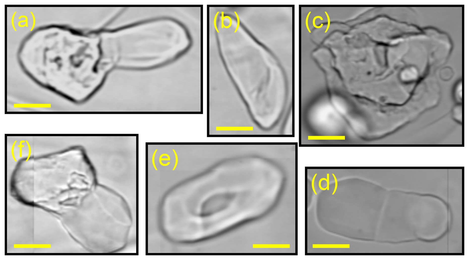
Figure 9 Example of complex-shaped air hydrates. (a) Cloud-like air hydrate with protrusion from 1285 m. The equivalent-circle diameter (D) is 286 µm. (b) Disk-like (flat?) air hydrate from 1285 m (D=189 µm). (c) Cloud-like (porous?) air hydrate from 1355 m (D=325 µm). (d) Disk-like (flat?) air hydrate from 1355 m (D=247 µm). (e) Hollow ring-shaped air hydrate from 1405 m (D=179 µm). (f) Cloud-like air hydrate with protrusion from 1566 m (D=202 µm). Scale bars correspond to 100 µm.

4.1.2 Climate signal and depth variations in N_ah and $\stackrel{\mathrm{‾}}{D}$ from 2415–2771 m

The average N_ah for samples from 2415–2496 m is 282 cm⁻³, which indicates that they belong to a cold period (probably MIS 6). This is in line with measured δ¹⁸O values (Oerter et al., 2025) and small ice grain sizes (Weikusat et al., 2009) (Fig. 5a and d). The air hydrates' mean diameter for these samples, however, is evidently overestimated (triangular markers in Fig. 6a) and therefore deviates from the climate dependence. For samples at 2535 and 2545 m, the N_ah decreases to 203 and 144 cm⁻³, respectively, which could indicate a climatic transition. From 2392–2545 m (region 2 in Figs. 5 and 8), we observe an increase in clusters containing two or more individual air hydrates, whose diameter is typically in the range of the samples $\stackrel{\mathrm{‾}}{D}$ (Fig. 10). We define clusters consisting of two air hydrates as “simple” (Fig. 10a) and clusters consisting of more than two air hydrates as “multi” (Fig. 10b and c). Multi-clusters are especially common in depth region 2. The observation of these clusters explains the overestimation of the mean diameter, as our image analysis method cannot distinguish between “one” air hydrate and clustered “many” air hydrates. Furthermore, the emerging of the latter explains the high mean volume and the abnormal volume concentration and TAC_h (Fig. 7a and b), as the volume of the cluster is overestimated during calculation of the volume from an area assuming a spherical shape. Besides the overestimation in volume, the increase in air hydrate clusters also leads to an underestimation of N_ah. However, quantification is challenging due to the difficulty in distinguishing individual air hydrate crystals within clusters from the images. Another indicator for increasing air hydrate clustering is the jump in the RSD of the mean diameter distribution between 2385–2392 m depth (Fig. 5c).

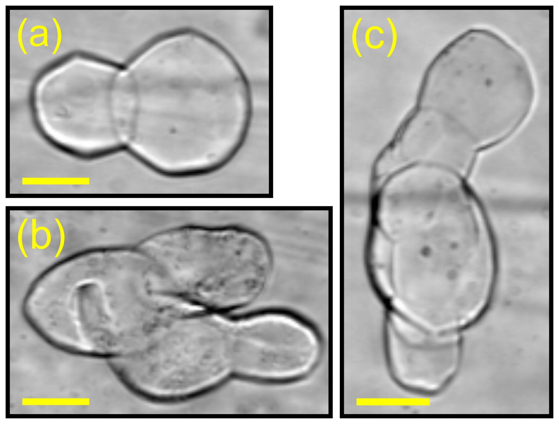
Figure 10 Example of clustered air hydrates in the sample from 2405 m depth. Scale bars correspond to 100 µm. Panel (a) represents a “simple” clustered air hydrate, and panels (b) and (c) represent “multi” clustered air hydrates. The equivalent-circle diameter for panels (a–c) is 257, 299, and 296 µm, respectively, which is about 2 times the samples $\stackrel{\mathrm{‾}}{D}$ (137 µm).

Below about 2550 m, both the N_ah and the mean size clearly deviate from the paleoclimatic influence (gray circles in Fig. 6b). On the one hand, this could be due to the increasing large-scale disturbances affecting the integrity of the δ¹⁸O record at this depth (Ruth et al., 2007; Faria et al., 2010a). On the other hand, air hydrates in deep ice are known to be affected by crystal growth, which can alter the climate-dependent variations in N_ah and mean size (Salamatin et al., 2003; Uchida et al., 2011). Evidence for air hydrate growth at EDML from about 2550 m is the decrease in the N_ah to the lowest values, and, simultaneously, the increase in the $\stackrel{\mathrm{‾}}{D}$ to the highest values, of the entire record (Fig. 5). Furthermore, N_ah and $\stackrel{\mathrm{‾}}{D}$ show a low variability, the air hydrates' mean volume increases steadily (Fig. 7a), and the air hydrates' aspect ratio decreases (i.e., they become increasingly spherical; Fig. 8b and c).

Air hydrate growth and the subsequent disappearance of the relationship between δ¹⁸O and air hydrate properties were reported for ice deeper than 2500 m at Dome Fuji (i.e., older than 350–400 kyr; Uchida et al., 2011), deeper than about 3300 m at Vostok (i.e., older than 300–400 kyr; Lipenkov et al., 2019), and for about 250 m from the bottom of the GRIP ice core in Greenland (Pauer et al., 1999; Salamatin et al., 2003). The fundamental reason behind the disappearance of climate-related variations in N_ah and $\stackrel{\mathrm{‾}}{D}$ is the fact that air hydrate growth rates are inversely proportional to the cube of their mean initial size (Salamatin et al., 2003). In other words, the growth rates of air hydrate ensembles with smaller mean size are higher than growth rates for ensembles with a larger mean size. Other parameters that influence air hydrate growth are increasing depth (and pressure), increasing age, and increasing ice temperature (Uchida et al., 2011).

For the EDML ice core, the age of the ice deeper than 2415 m is not known. However, the sudden increase in ice grain size by 1–2 orders of magnitude to up to 0.5–1 m for the deepest samples (Faria et al., 2010a; Weikusat et al., 2017) and the relatively warm in situ ice temperature of −8°C at about 2550 m (Fig. 8d) indicate favorable conditions for air hydrate crystal growth. Thus, we interpret our data to mean that, from this depth, the climate signal is dampened by considerable air hydrate crystal growth.

The reason for the absence of air hydrates in the lowermost sample at a depth of 2773.91 m, that is, about 25 cm above the bottom of the ice core, is currently unclear. The bottom of the core reaches the pressure melting point (−2°C; Faria et al., 2010a), and ice core drilling was terminated because subglacial water entered the borehole (Wilhelms et al., 2014). Furthermore, Faria et al. (2010a) reported that, from 2760 m, the concentration of microinclusions gradually decreases with depth. Therefore, the sample could represent accreted ice with no or very few impurity inclusions (at least in the 10 cm sample). On the other hand, the ice could be of meteoric origin and subject to processes that resulted in the expulsion of impurities and gases, i.e., the segregation of impurities to the grain boundary network and subsequent drainage to the bedrock driven by the hydraulic gradient (Rempel et al., 2002; Rempel, 2005). These processes are considered to alter the basal ice at EDC (Tison et al., 2015), Dome Fuji (Ohno et al., 2016), and NEEM (Goossens et al., 2016). Note that a decrease in TAC was only reported (or measured) for samples of the NEEM ice core (Goossens et al., 2016). Further investigations of the deepest ice at EDML are necessary to determine its origin and explain the absence of air hydrates.

4.2 Influence of ice deformation and microstructure on the air hydrate ensemble

4.2.1 Region 1: 2025–2115 m

For this depth range, corresponding to region 1, we observe an inverse behavior of N_ah and $\stackrel{\mathrm{‾}}{D}$ to what would be expected based on the δ¹⁸O record (Fig. 5a–c). On top of that, we observe a sudden increase in air hydrate aspect ratio and a rotation of their major axis towards the horizontal between 2005–2035 m, i.e., at the beginning of the mismatching region.

At approximately 2030 m depth, Weikusat et al. (2017) observed an abrupt change in the ice crystallographic preferred orientation (CPO) from a vertical girdle to a single maximum (indicated in our Fig. 8d) and attribute this observation to a transition from a pure shear to a simple shear-dominated deformation regime. Additionally, inclined and undulating cloudy bands on the millimeter (mm) to centimeter (cm) scale (i.e., a disturbed stratigraphy) and the onset of an echo-free zone in radio-echo sounding measurements were observed from about 2050 m depth (Drews et al., 2009; Faria et al., 2010a, b). We surmise that the simultaneous occurrence of the abrupt change in ice crystal properties, as a consequence of the change in overall deformation regime, and the change in air hydrate shape parameters is linked.

Durham et al. (2010) summarized the rheological behavior of certain sI and sII gas hydrates measured in laboratory deformation tests and found them to be several orders of magnitude stronger than ice. Cao et al. (2020) performed molecular simulations to assess the mechanical behavior of ice-contained methane hydrates (sI) and found their partial dissociation and reformation due to mechanical deformation. Therefore, we suspect that air hydrates in ice could be seen as an analog to porphyroclasts in rocks, which are single (mineral) grains that have a different rheology than the surrounding matrix. Porphyroclasts may be rigid, deformable, or weaker than their surrounding matrix and have the ability to recrystallize, rotate, or elongate and obtain a stable position in the extensional quadrant of flow (e.g., Passchier and Trouw, 2005). The increase in air hydrate aspect ratio and their rotation towards the image x axis (shear plane?) from about 2035 m could be caused by crystal plastic deformation combined with rigid body rotation and matches well with the change towards a simple shear-dominated deformation regime, considering the aforementioned behavior of porphyroclasts in rocks.

An additional explanation could be that air hydrates preferentially elongate along the basal plane of ice crystals. Using molecular dynamics simulations, Factorovich et al. (2019) found that the (111) lattice plane of the sII hydrate can bind to the basal plane of hexagonal ice through domain matching to produce epitaxy and alignment between these crystals. Similarly, a strong connection of the ice crystal basal plane and air bubble elongation was found by Fegyveresi et al. (2019). Considering the CPO change to a single maximum, a preferred elongation of air hydrates along the basal plane of ice crystals could explain the sudden rotation towards the image x axis between 2005–2035 m.

The air hydrates' elongation and alignment towards the horizontal persist down to 2395 m depth and could be explained by the abovementioned mechanisms. The strong anomaly in N_ah and $\stackrel{\mathrm{‾}}{D}$, however, is restricted to 2025–2115 m. Whether the change in deformation regime can cause a localized air hydrate growth due to a change in the air molecule diffusion rate caused by an increase in interstitials and lattice defects in the ice matrix, for instance, requires further investigations.

4.2.2 Region 2: 2392–2545 m

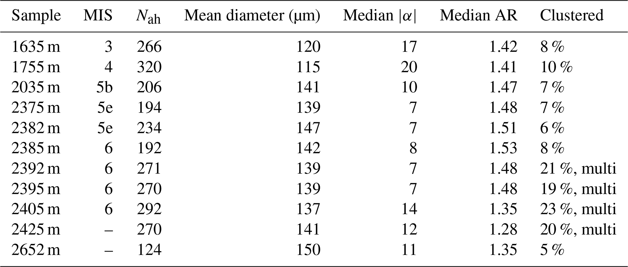
For this depth range, corresponding to region 2, we observe an increase in air hydrate clusters, which cause an overestimation of the mean diameter (Figs. 5 and 6a and Table 3). On the one hand, the air hydrate clusters could form from fragmentation of larger, “out-of-equilibrium” air hydrates. On the other hand, they could form due to coalescence, which occurs when encountering air hydrates merge in order to reduce their total interfacial area (Uchida et al., 2011). We suspect the latter: firstly, the depth region from 2385–2495 m corresponds to a cold climate and, as a result, should contain (and does contain) a higher number of relatively smaller air hydrates. Secondly, the diameter of the individual air hydrates forming the clusters is in the range of the samples $\stackrel{\mathrm{‾}}{D}$ (Fig. 10), and, thirdly, the majority of air hydrates are rounded and have a low aspect ratio (Fig. 8b and c). As a prerequisite for coalescence, air hydrate crystals need to migrate through the ice matrix, and one underlying mechanism could be dragging due to grain boundary migration during ice crystal growth (Uchida et al., 2011). The ice core depth region from 2392–2545 m seems predestined for such a process. The appearance of a distinctive ice microstructure (“brick wall pattern”) is evidence for strain accommodation via grain boundary sliding (Faria et al., 2009). Moreover, from 2405 m to about 2600 m, cloudy bands are inclined, and folding and other stratigraphic disturbances are frequent (Faria et al., 2010a, b). These observations are indicators for high strain rates and a bed-parallel (simple) shear-dominated deformation regime (Faria et al., 2010a; Weikusat et al., 2017).

Table 3 Air hydrate parameters for selected samples from MIS 3–5 and from the penultimate glacial–interglacial transition zone. We used randomly selected air hydrates belonging to the “in focus” visual category (A, C in Fig. 1) to determine the number of clustered air hydrates. The number of randomly selected air hydrates is equal to the samples' N_ah.

5 Conclusions

We present a new method to analyze air hydrate crystals in high-resolution microphotographs of polished ice thick sections using automated image segmentation and analysis. This new image analysis approach allows an efficient evaluation of large amounts of image and air hydrate data and eliminates the need for tedious manual counting. We analyzed air hydrates included in 74 samples of the EDML ice core over a depth range from 1255–2771 m, which were acquired in the field (years 2003–2006) shortly after the ice core was drilled. We measured the number of air hydrates in each sample and characterized their sizes and shapes to obtain depth profiles of the number concentration (N_ah), mean diameter ($\stackrel{\mathrm{‾}}{D}$), volume concentration (V_c), aspect ratio (AR), and orientation (α). The measured variations in N_ah and mean diameter with depth clearly resolve the MIS 4 stadial period and the penultimate glacial-to-interglacial transition. Consequently, we confirm the general relation of the air hydrate properties with past climate, as shown previously for the Dome Fuji (e.g., Ohno et al., 2004), Vostok (e.g., Lipenkov, 2000), and GRIP (Pauer et al., 1999) ice cores. We also confirm that air hydrates grow with depth (time) based on the observed decrease in N_ah and corresponding increase in mean size (i.e., mean volume) following an Ostwald ripening process. We estimate the growth rate from 1255–2405 m, which corresponds to the dated depth region of the EDML ice core, to be $\mathrm{8.0}\times {\mathrm{10}}^{-\mathrm{12}}{\mathrm{cm}}^{\mathrm{3}}$ per year. Besides Ostwald ripening, locally increased air hydrate coalescence causes a minor decrease in N_ah and an increase in mean diameter in the depth range of 2392–2545 m. From about 2550 m down to the bottom, the climatic control on the air hydrate ensemble is disturbed by air hydrate growth, which coincides with observations from the GRIP ice core (Pauer et al., 1999; Salamatin et al., 2003).

The connection between the δ¹⁸O and air hydrate records is not always resolved on the small scale at EDML. To pinpoint the reasons, detailed studies on, for example, the mechanisms for the air bubble–air hydrate transition are required. They should be carried out as soon as possible after drilling the ice core (Pauer et al., 1999; Kipfstuhl et al., 2001).

The EDML ice core was drilled on an ice divide and has a distinctive ice microstructure interpreted as the effects of changing boundary conditions of deformation (Weikusat et al., 2017). Remarkably, our air hydrate shape profiles, expressed as variations in median AR and median $\left|\mathit{\alpha }\right|$, reflect the change from a pure shear to a simple shear-dominated deformation regime at about 2030 m as discussed by Weikusat et al. (2017). We observe a sudden increase in air hydrates' AR and in the rotation of their major axis towards the horizontal. Furthermore, increased air hydrate coalescence from 2392–2545 m coincides with a bed-parallel shear-dominated region exposed to high strain rates (Faria et al., 2010a; Weikusat et al., 2017). For this reason, we are convinced that the air hydrate ensemble is substantially influenced by ice deformation and/or the resulting ice microstructure. Identifying the mechanisms behind the interaction of air hydrates and ice (deformation), and whether these mechanisms can also cause the pronounced deviation of the climatic influence observed from 2025–2115 m depth, should be investigated in future studies.

The scientific results, methods, and workflows to analyze air hydrates in microphotographs described in this work will assist us in improving our understanding of air hydrates and their properties in ice cores and can be useful to further develop a novel dating tool based on air hydrate crystal growth (Lipenkov et al., 2019).

Appendix A: Image data

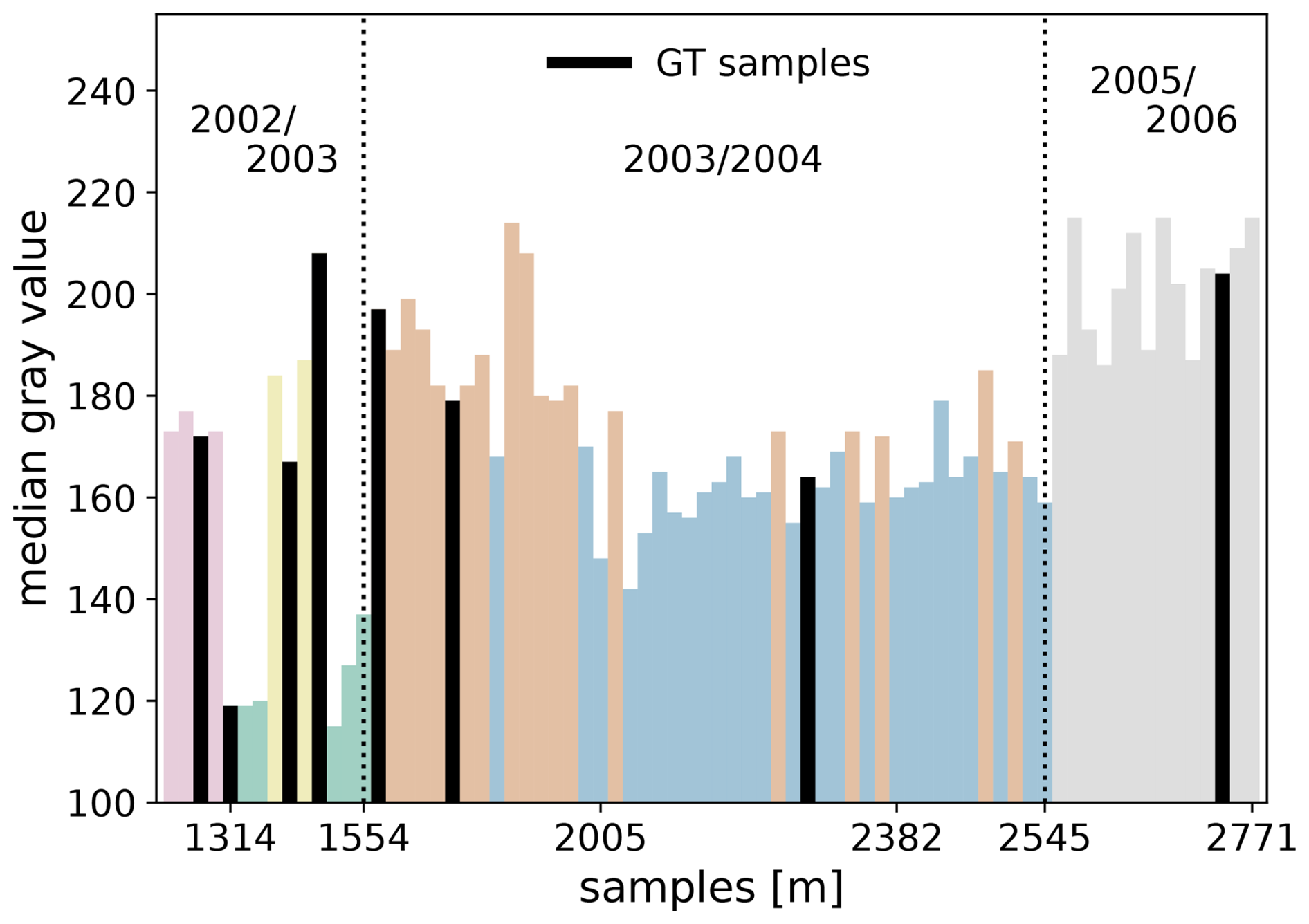
Figure A1 Selected samples and their median gray value (i.e., brightness) acquired during three Antarctic field seasons in the depth range from 1255 to 2771 m. The different colors correspond to the six image categories, and the black bars mark the samples where a section of the sample was used as ground truth image.

Appendix B: Image analysis

B1 Air hydrate segmentation

The Canny edge detection algorithm (Canny, 1986) is the core of this image segmentation routine. It is a multi-stage edge detector and is implemented in scikit-image (van der Walt et al., 2014) in the following way: in a first step, the image is smoothed by a Gaussian filter to reduce noise. Next, the intensity gradients of the image are calculated, of which only the maxima are identified as potential edges. At last, a hysteresis thresholding on the gradient magnitude is applied. Edges with an intensity gradient above a maximum threshold are true edges, and those below a minimum threshold are non-edges. Those who lie between these two thresholds are classified true edges or non-edges based on their connectivity. If they are connected to “true-edge” pixels, they are considered to be part of edges. The prediction of true edges via hysteresis thresholding depends a.o. on the image brightness. To account for the different imaging conditions, we kept the minimum threshold at zero, while the optimal maximum threshold was determined for each of the six image categories by optimizing the segmentation metrics for ground truth (GT) images. For this, we prioritized precision over recall to avoid over-segmentation (see Sect. 2.4).

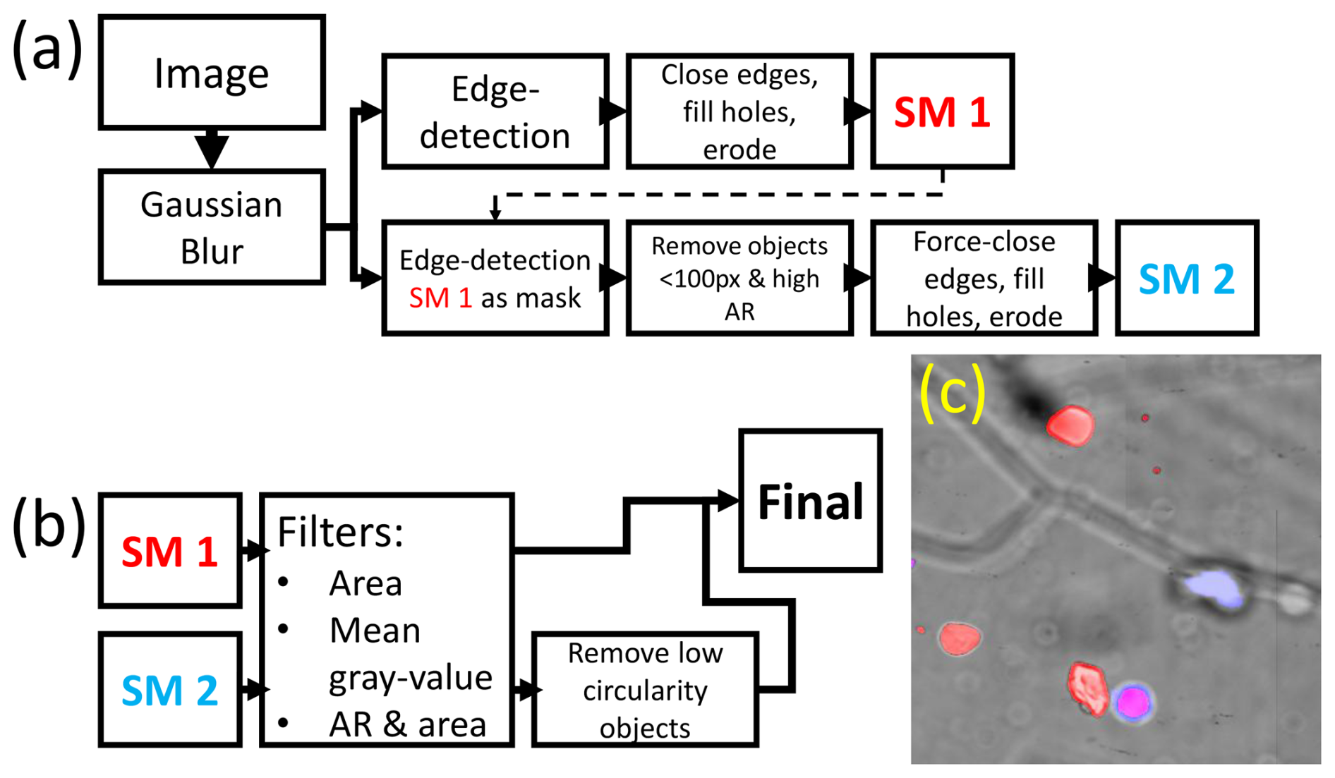
Figure B1 Detailed segmentation (a) and filtering (b) steps. Panel (c) shows SM 1 and SM 2 after the segmentation step (a) on top of the original image.

The Canny edge detection operation produces a binary edge map, and an example result is shown in Fig. 2b. In a first segmentation step, a morphological closing (1 px as structuring element), a “fillholes” operation, and an erosion (by 1 px) operation are applied to the edge map to obtain a first binary image of well-segmented objects (Segmented Mask 1 = SM 1 in Fig. B1a, red objects in Fig. B1c). Next, SM1 is used as a mask for another edge detection operation in a second segmentation step. From the resulting edge map, objects with a small area and a high aspect ratio (usually erroneously segmented grain boundaries) are removed before a “force-closing” operation (disk with r=3 px as structuring element), a “fillholes” operation, and an erosion operation are applied to produce a second mask (SM 2 in Fig. B1a, blue objects in Fig. B1c). Ultimately, a set of filters is applied to the resulting SM 1 and SM 2 images to remove common artifacts (e.g., I–V in Fig. 1) before combining them to the final segmentation result (Fig. 2c).

B2 Segmentation evaluation with ground truth images

Table B1 Comparing ground truth and segmentation results. The table headers correspond to air hydrate visual categories (see Table 1).

Appendix C: Projection properties of ellipsoids

Figures C1–C3 show the changes in orthogonal projection properties of an ellipsoid that is rotated around the core axis (Z). A and C of the ellipsoid correspond to the major and minor axis of the projected ellipse and are the same for the three initial conditions (Figs. C1a, C2a, and C3a). The third dimension, B, is changed accordingly to represent three end-member cases.

One challenge in the interpretation of shape and orientation data lies in the fact that we do not know if we measured the maximum elongation and that the third dimension is unknown, i.e., if the non-isometric object is more cigar (prolate)-like (e.g., Fig. C2) or more oblate-like (e.g., Fig. C3). For the interpretation of the air hydrate shape characteristics, we consider the relative orientation of the ice samples to each other. As mentioned in Sect. 2.5.2, a change in relative orientation could be caused due to a difficulty in matching core breakpoints during ice core logging.

Weikusat et al. (2017) report a loss in azimuthal orientation of the core between 1686–1696 m and between 1955–2035 m depth. Between 1665–1695 m, we observe an increase in air hydrate median orientation from 17 to 22° (Fig. 8b) and a “polarity” change (Fig. C4a and b). However, we do not observe a significant change in the median AR (Fig. 8b). Between 2005–2035 m depth, we observe a more continuous decrease in the median orientation (Figs. 8b and C4c–e) and an increase in the median AR (Fig. 8b). The fact that the median AR does not change between 1665–1695 m, while the orientation does, implies either that the air hydrates are not very well sorted or that the majority is rather isometric in shape. On the contrary, the continuous and joint change in AR, together with orientation from 2005 to 2035 m depth, points towards either an increase in sorting or a decrease in isometric air hydrates. Both could be induced by the increase in simple shear deformation.

Future work should consider taking images from two (or more) different directions to increase the accuracy in air hydrate shape and orientation measurements.

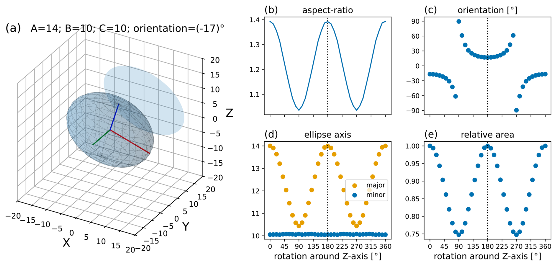
Figure C1 Panel (a) shows an ellipsoid together with its projection to the XZ plane, which corresponds to the image plane of the microphotograph (cf. Fig. 1). A = 14 (red), B = 10 (green), and C = 10 (blue) are the ellipsoids' axes, and the orientation is the angle (−17°) between the semi-major axis (a) and the X axis. Panels (b–e) show the evolution of the aspect ratio, the orientation, the major and minor axis, and the relative area with progressing rotation around the Z axis (core axis) from 0°, initial condition in panel (a), to 360°.

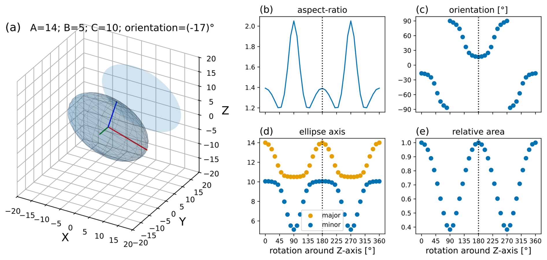
Figure C2 Panel (a) shows an ellipsoid together with its projection to the XZ plane, which corresponds to the image plane of the microphotograph (cf. Fig. 1). A = 14 (red), B = 5 (green), and C = 10 (blue) are the ellipsoids' axes, and the orientation is the angle (−17°) between the semi-major axis (a) and the X axis. Panels (b–e) show the evolution of the aspect ratio, the orientation, the major and minor axis, and the relative area with progressing rotation around the Z axis (core axis) from 0°, initial condition in panel (a), to 360°.

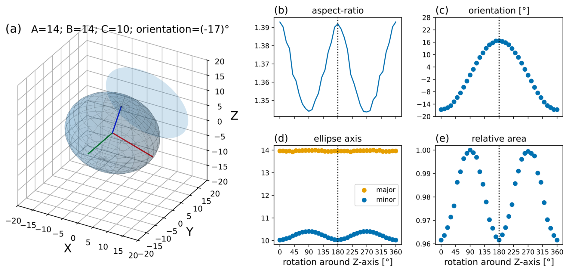
Figure C3 Panel (a) shows an ellipsoid together with its projection to the XZ plane, which corresponds to the image plane of the microphotograph (cf. Fig. 1). A = 14 (red), B = 14 (green), and C = 10 (blue) are the ellipsoids' axes, and the orientation is the angle (−17°) between the semi-major axis (a) and the X axis. Panels (b–e) show the evolution of the aspect ratio, the orientation, the major and minor axis, and the relative area with progressing rotation around the Z axis (core axis) from 0°, initial condition in panel (a), to 360°.

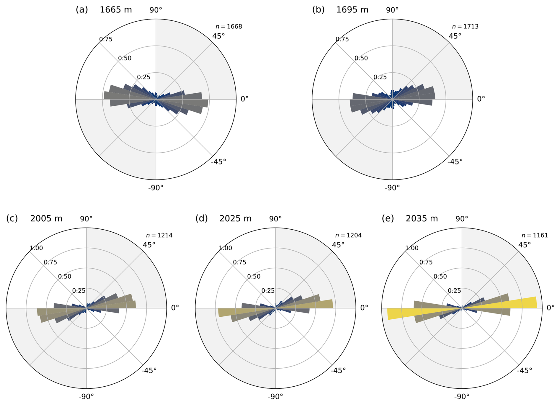
Figure C4 This figure shows orientation plots (“rose plots”) of the air hydrate major axis for samples from (a) 1665 m, (b) 1695 m, (c) 2005 m, (d) 2025, and (e) 2035 m depth. “n” corresponds to the number of measured objects for each sample, i.e., objects with an AR higher than 1.33.