Monitoring shear-zone weakening in East Antarctic outlet glaciers through differential InSAR measurements

The stability of the Antarctic Ice Sheet depends on ice flux into the ocean through major outlet glaciers, which is resisted by shear stresses in the lateral shear margins, both on grounded ice and on floating ice shelves. Within the tidal-flexure zone, where the ice sheet transitions from fully grounded to freely floating, ocean tides lead to a characteristic flexural pattern, which can be detected by radar satellites in differential interferograms. Here, we investigate how spatially heterogeneous elastic ice-shelf properties in the shear zones affect tidal flexure and whether a corresponding signature can be detected in satellite observations. We use the Young's modulus (which, among others, depends on ice temperature and/or ice-crystal orientation fabric and damage) as a bulk tuning variable for changing ice stiffness across shear zones and show that this leads to centimeter-scale deviations in vertical displacement, compared with a homogeneous elastic flexure model. Using the tidal-flexure zone of Priestley Glacier as an example, we compare homogeneous and heterogeneous flexure-model predictions with observations from 31 differential interferograms. After adjusting the local tide model and validating it with in situ GPS data, we find that a 5-fold reduction of the Young's modulus in the shear zone, i.e., an effective shear-zone weakening, reduces the root-mean-square error of predicted and observed vertical displacement by 33 % within the central part of the ice shelf. This suggests that satellite interferometry can detect changing ice stiffness across shear zones, with the potential to inform ice-flow models about the often unknown spatial variability in ice-shelf properties along the grounding zone.

1 Introduction

1.1 Context and research question

Outlet glaciers transport ice from the interior of the Antarctic Ice Sheet to the coast, where ice crosses the grounding line and forms floating ice shelves. Ice shelves are largely in hydrostatic equilibrium with the ocean, apart from a few-kilometers-wide belt just seaward of the grounding line, where the ice continuously flexes between the fully grounded and the fully floating areas. The pattern of the vertical displacement arising from this flexure has stirred much previous research, for example, because it modulates the dynamics of tributary ice streams (Anandakrishnan et al., 2003; Gudmundsson, 2006; Murray et al., 2007), because it may foster exchange of subglacial and ocean water (Walker et al., 2013; Warburton et al., 2020; Robel et al., 2022; Bradley and Hewitt, 2024), because it reveals tidal grounding-line migration (Freer et al., 2023), and also because the ice here is not in hydrostatic equilibrium and so confidently deriving ice thickness at the grounding line from satellite altimetry is a significant challenge (Fricker and Padman, 2006; Fricker et al., 2009). Here, we explore whether the vertical displacement by tides can be used as a natural experiment to highlight spatially variable ice-shelf properties resulting in spatially variable ice stiffness. For example, if the ice stiffness varies spatially and is lower in the lateral shear margins than elsewhere, this would reduce ice-shelf buttressing of the upstream ice flow, relative to a homogeneous case.

1.2 Previous work

Previous research has provided much progress in understanding tidal flexure and its ice-dynamic implications, both in modeling and observations. In terms of observations, satellite coverage and resolution have proliferated in the last decades (e.g., Friedl et al., 2020) using altimeters (e.g., Li et al., 2022; Freer et al., 2023) and interferometric synthetic aperture radar imaging (InSAR; Rignot et al., 2019; Milillo et al., 2019, 2022; Rignot et al., 2024). Most relevant for this study are differential InSAR applications (DInSAR, Rignot et al., 2011), which image tidal flexure even in regions with minimal tidal range, such as the Ross Sea (Padman et al., 2018). As explained in more detail later, this technique captures the spatial extent of the tidal-flexure zone and reliably marks the landward and seaward limits of tidal flexure, typically within fractions of the local ice thickness (Brunt et al., 2010). Modeling tidal flexure and its ice-dynamic implications is challenging because all stress terms in the full Stokes equations might be relevant (Rosier and Gudmundsson, 2018) and also because tidal timescales require the consideration of elastic properties together with viscous deformation (Reeh et al., 2000, 2003; Gudmundsson, 2011; Wild et al., 2017). Nevertheless, this approach has led to important findings, for example, in terms of the subglacial hydrology (Hewitt, 2013; Walker et al., 2013; Rosier and Gudmundsson, 2020) and stress coupling across the grounding line (Rosier and Gudmundsson, 2016).

The lateral shear margin of a glacier is a region of large deformation that separates the fast-flowing ice from stagnant ice or rock. Shearing within lateral margins leads to a resistive force (side drag) that counteracts a large proportion of the glacier driving stress. The nature of this side drag depends on local ice rheology, which changes as a function of damage, temperature, melting, and ice fabric, and these in turn depend on the local shearing (Minchew et al., 2018). Despite their important role in regulating glacier flow, shear margins are a relatively poorly understood component of glaciers due to the numerous challenges in accessing and measuring these complex regions.

1.3 Current shortcomings

Rifts develop along lateral shear zones due to rapid shearing and localized strain (Alley et al., 2019). These surface rifts pose challenges for in situ data collection (Arcone et al., 2016), limiting the availability of observational data needed to validate remote-sensing methods (Marsh et al., 2021). The situation is further complicated by significant surface velocity gradients, which cause phase decorrelation in InSAR processing. As a result, monitoring fast-flowing glaciers and ice streams, such as Thwaites Glacier (Milillo et al., 2019; Rignot et al., 2024) and the Dotson–Crosson ice shelf system (Milillo et al., 2022), is only possible via lower-resolved SAR amplitude tracking when using publicly available satellite SAR data, which typically have repeat passes of multiple days to weeks. Addressing this issue requires dedicated satellite missions with shorter repeat acquisition intervals (hours to days) to ensure phase coherence for fast-flowing areas and particularly across shear zones. This limitation currently hinders an Antarctic-wide assessment. Future advancements in satellite radar technology are expected to enhance the temporal resolution of publicly available SAR data, improving their ability to capture the flexural response across shear zones and advancing our understanding of ice-shelf dynamics. It is therefore necessary to develop methods that infer spatially variable ice properties indirectly.

1.4 Framework of this paper

Here we investigate whether the heterogeneity in ice stiffness can be observed along the tidal-flexure zone but, instead of using the horizontal velocities as primary observations, we compare the observed vertical displacement with an elastic flexure model. We use a spatially variable Young's modulus as a proxy for heterogeneous ice temperature, ice fabric, and damage. Ice that is warmer or in which the ice fabric is aligned with the principal ice-flow direction will deform more strongly for a given stress regime than its cold and isotropic counterparts (Hudleston, 2015). In the elastic model, we approximate this weakening with a lowered Young's modulus. As we will show later, a spatially heterogeneous Young's modulus leads to a nonlocal response in the prediction of tidal flexure; misfits between predictions and observations can be used to diagnose such spatial heterogeneities from satellite observations.

The study is structured as follows. First, we test the hypothesis that reducing ice stiffness within lateral shear zones can exert a detectable signal in DInSAR mappings. If substantiated, this hypothesis implies that DInSAR imagery can offer insights beyond the conventional delineation of grounding lines, providing additional information about ice properties. Second, we use repeat-pass satellite measurements from DInSAR to constrain an elastic model of tidal flexure. Using the flexural response of floating ice near the grounding line to tidal forcing as a regional experimental setting, we reveal bulk softening in ice-shelf shear zones. This insight is derived from a comparison between homogeneous and heterogeneous model experiments and satellite-derived tidal-flexure patterns of Priestley Glacier. Third, we challenge our assumption of elasticity by incorporating in situ data of surface deformation recorded both outside and within the tidal-flexure zone.

2 Hypothesis and study area

2.1 Synthetic model experiments

We begin by conducting synthetic modeling experiments to illustrate the hypothesized effects of shear-margin weakening on the tidal-flexure patterns of an idealized outlet glacier. The synthetic ice thickness profile we use is broadly consistent with the known geometry of Priestley Glacier. Specifically, we assume ice thickness of 1000 m at the grounding line, tapering nonlinearly to 500 m at the ice edge, following the model geometry described by Holland et al. (2008) and formulated by Walker et al. (2013):

$$\begin{array}{}\text{(1)}& H={\mathit{\beta }}_{\mathrm{1}}/{\left({\mathit{\beta }}_{\mathrm{2}}-\left(x-x_{\mathrm{gl}}\right)\right)}^{\mathrm{1}/\mathrm{2}},\end{array}$$

where H represents ice thickness, while parameters β₁ and β₂ are adjusted to control the ice thickness at the grounding line and ice edge. The model spans a domain of 12 km × 25 km, incorporating a sinusoidal grounding line to reflect the geometric features within a landward embayment (Fig. 1a).

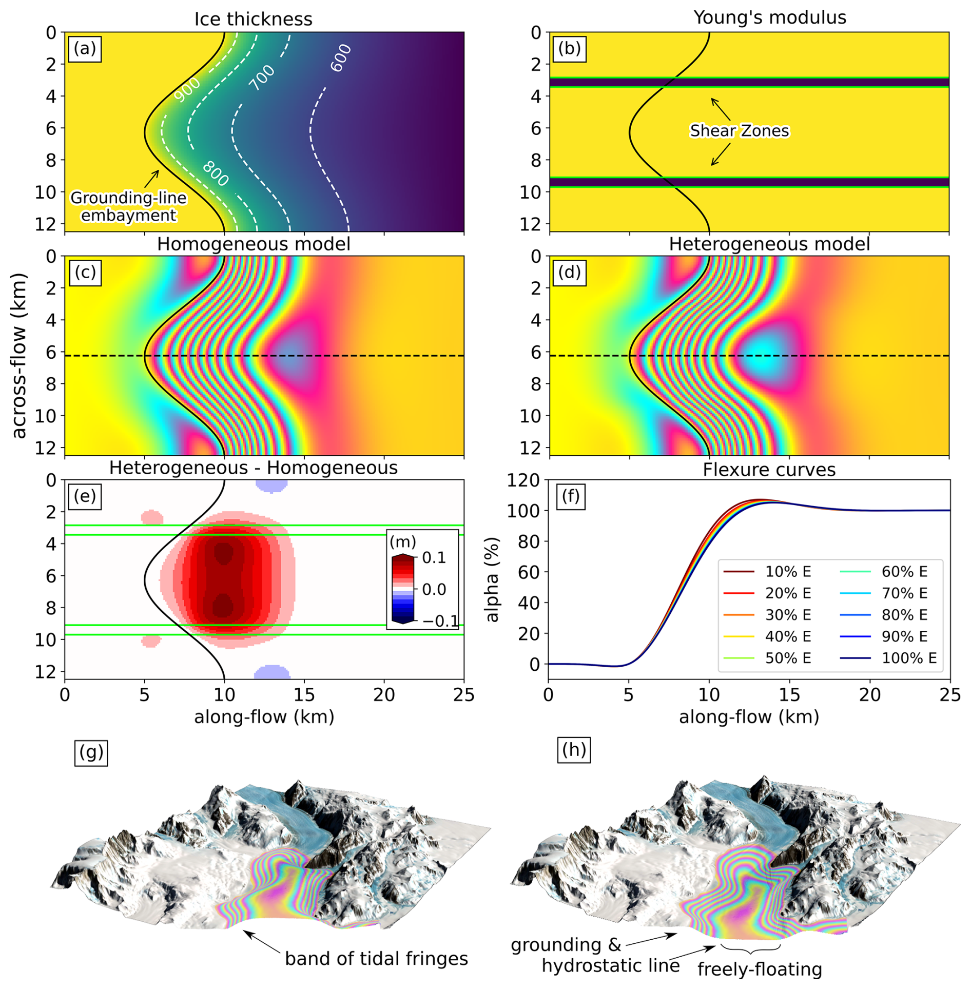
Figure 1 Hypothesis. (a) Idealized ice thickness for synthetic model experiments. (b) Young's modulus field, where values are varied in the shear-zone areas (shown in blue) in steps of 10 % from 10 % to 100 % of the Young's modulus used for the remaining ice-covered areas (indicated in yellow), which is set at 1.6 GPa. (c, d) Modeled tidal flexure under 1 m tidal forcing for (c) a homogeneous case and (d) a heterogeneous case. (e) Their difference, showing a bulge of up to 10 % of the applied tidal forcing. (f) Cross-section along the centerline (dashed lines in panels c and d), illustrating the flexure curves where Young's modulus is reduced in lateral shear zones. (g, h) Vertical tidal flexure during (g) high-tide and (h) low-tide scenarios. Each color fringe represents approximately 10 cm of vertical displacement, corresponding to a tidal amplitude of ±60 cm in this schematic. The concentrated band of tidal fringes marks the grounding line at its landward edge and the hydrostatic line at its seaward boundary. Beyond this, the ice floats freely on the ocean, oscillating harmonically with the tides. Note that vertical displacement is not to scale in this schematic.

We model the expected vertical deformation due to ocean tides with a peak amplitude of 1 m using an elastic model, the details of which are explained in Sect. 3.3. Our baseline simulation, against which all other simulations are compared, assumes spatially homogeneous elastic properties, represented by a constant Young's modulus (E). Spatial heterogeneity is introduced within the floating parts in the form of two localized regions with a lower Young's modulus on either side of the model domain (Fig. 1b). Contour lines of vertical displacement for any time interval in a tidal cycle are visualized with a cyclic color map (Fig. 1c and d; here, specifically, one color cycle, or one fringe, corresponds to 10 cm). Such color maps are commonly used in satellite interferometry, which we will use later as our main source of observations.

We find that introducing elastic heterogeneity leads to a nonlocal response in tidal flexure, which is expressed in contrast with the homogeneous case in the form of a distributed bulge, most prominently in the ice-shelf center (Fig. 1e). More specifically, the degree of hydrostatic balance (i.e., the ratio of ice deformation over tidal deformation, denoted α, where 0 % depicts fully grounded and 100 % depicts fully floating ice) changes with the strength of the heterogeneity (Fig. 1f). This suggests that the tidal-flexure pattern can be used as a proxy to extract bulk heterogeneity. The magnitudes involved (typically <10 cm) are within the sensitivity of satellite interferometry but tide models will need to be constrained with in situ data that are available for our research area. We therefore move to the real-world geometry of Priestley Glacier (Fig. 1g and h). If our hypothesis regarding effective shear-zone weakening is correct, we expect to detect a similar bulge in the difference fields of various model scenarios and the observed tidal-flexure patterns from differential satellite interferometry (DInSAR). This would provide additional insights into the spatial variability of ice rheology, extending beyond the traditional use of DInSAR for monitoring grounding lines.

2.2 Study area

Priestley Glacier is a 96 km (60 mi) long outlet glacier in Victoria Land, East Antarctica, originating from the edge of the polar plateau. It flows through the Transantarctic Mountains, draining into the fjord-like grounding zone of the Nansen Ice Shelf in Terra Nova Bay (Fig. 2). The glacier features floating shear zones with long-term shear strain rates around 0.01 yr⁻¹ (Fig. S1 in the Supplement). A stake network survey conducted on the glacier's true left shear zone revealed spatial variability in ice stiffness, with softer ice in the shear zone and stiffer ice in the central part of the glacier (Still et al., 2022). Observations also identified localized tidal flexure, which could only be modeled by incorporating a spatially heterogeneous Young's modulus or modifying the boundary conditions to account for coupling with a rocky ridge on the glacier's left sidewall. Ice core measurements taken from the same area showed that grain size reduction and preferential c-axis alignment, consistent with shear deformation along a vertical shear plane perpendicular to the flow direction, contributed to the mechanical ice softening (Thomas et al., 2021).

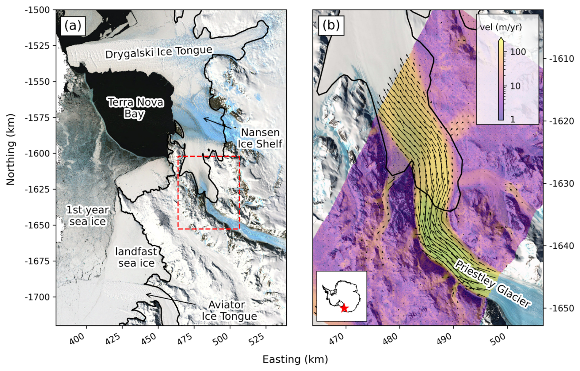
Figure 2 Landmarks along the Victoria Land coast of East Antarctica. (a) The dashed red rectangle shows the location of the study area in panel (b). (b) The transitioning zone of Priestley Glacier, draining into the Nansen Ice Shelf, superimposed with a velocity field derived from TerraSAR-X data in 2018. The map background is the Landsat Image Mosaic of Antarctica (LIMA; Bindschadler et al., 2008). The grounding line is sourced from the Antarctic Surface Accumulation and Ice Discharge project (ASAID; Bindschadler et al., 2011). The inset shows the location of the study site along the Transantarctic Mountains in East Antarctica. Map coordinates are given in an Antarctic Polar Stereographic projection (EPSG:3031).

3 Data and methods

We seek to detect differences between modeled and observed vertical displacements throughout the tidal cycle. This requires adjustments of the tidal forcing used for predictions to overcome tide-model inaccuracies and a decomposition of the double-differential tidal displacement measured by DInSAR into a synthesized time series of “single-tide” displacements at the times of SAR data acquisitions. The process begins with deriving an α-map from DInSAR measurements, representing the average tide-deflection ratio. Next, the tide-model output is adjusted to align with DInSAR observations over the freely floating portion of the ice shelf. This adjusted tide model is then combined with the α-map to predict average tidal displacements at the times of SAR data acquisition.

These predicted tidal displacement maps are reassembled to compute residual mismatches for the original DInSAR images. Similar to the tide-model adjustment, we then determine the minimal per-pixel offsets needed in the average tidal displacement maps to best match the DInSAR data. By subtracting these offsets from the predicted tidal displacement maps, we effectively decompose the DInSAR images into their underlying “single-tide” components, enabling the reconstruction of synthetic displacement maps corresponding to each SAR data acquisition.

When these synthetic maps are again reassembled for comparison with the original DInSAR images, we refer to the resulting products as mosaics. In the following, we detail the individual steps for Priestley Glacier; an example for Darwin Glacier can be found in Wild et al. (2019). To assess the role of shear-zone weakening, we replace the α-map from DInSAR measurements with modeled α-maps from homogeneous and heterogeneous experiments. We validate model solutions with GPS data from two sites and find that incorporating any α-map significantly improves the fit between observed and modeled displacements. However, the GPS sites themselves are not particularly sensitive to the specific modeling choices; this motivates our broader evaluation across the entire tidal-flexure zone. Finally, the GPS records are also used to estimate the timing of tidal oscillations at the two sites to assess the validity of the elastic approximation.

3.1 Remote sensing of the tidal-flexure zone

3.1.1 Satellite-based surface velocity and DInSAR tidal flexure

TerraSAR-X is the highest resolution sensor (< 2 m in StripMap mode) employed in this study and we used it as a baseline to determine the surface velocities, the surface strain-rate field, and the grounding line. Surface velocities were based on speckle tracking of two SAR images from November 2018 using the Gamma software package (Werner et al., 2000). Corresponding strain rates were calculated using the strain-rate formulation (Alley et al., 2018). DInSAR images stem from double differencing three consecutive SAR scenes. The double differencing cancels the steady horizontal component of ice flow and contains two interferograms, which are calculated out of three overpasses (i.e., both interferograms have one joint SAR data acquisition in time). We used three SAR scenes, from 5, 16, and 27 June 2018, to compute one TerraSAR-X DInSAR image (Fig. S2), from which we delineated a grounding line located in an approximately 100 m wide grounding zone, where the grounding line migrates over a tidal cycle (Drews et al., 2021a). Additionally, we used 56 Sentinel-1 SAR scenes, acquired between May 2017 and July 2020, to create 31 DInSAR images of Priestley Glacier (see Neckel et al., 2021, for more detail). These images were phase unwrapped using a minimum-cost flow algorithm and show double-differential tidal displacement.

3.1.2 Derivation of an α-map from DInSAR measurements

From the 31 unwrapped DInSAR images, we selected a reference location 25 km downstream of the grounding line within the freely floating part of the ice shelf to measure double-differential tidal displacement. We synthesized the tidal-flexure pattern across multiple tidal cycles by calculating the mean ratio between the vertical displacement of each pixel in a DInSAR image and the double-differential tidal displacement of the reference. This empirically derived map then shows the temporally averaged tide-deflection ratio (α-map; Han and Lee, 2014), where values of 0 % indicate grounded ice and values of 100 % delineate freely floating areas. Intermediate values quantify the average degree of tidal flexing. An α-map thus shows the mean tidal flexure that can be expected for any tidal amplitude.

3.1.3 Tide-model adjustment with DInSAR

For our method, it is necessary that a tide model used to force the modeling matches the double-differential tidal displacement measured with DInSAR on the freely floating part of the ice shelf. Despite significant improvements in tide-model accuracy for coastal Antarctica – reduced from ±10 cm (Padman et al., 2002) to ±6.5 cm (Stammer et al., 2014) – this accuracy remains an order of magnitude lower than the millimeter-level precision of DInSAR (Rignot et al., 2011). Therefore, we treated DInSAR measurements of vertical displacement in freely floating areas as the reference standard and adjusted the tide-model output to align with these satellite observations.

We adjust the tide model at 56 time stamps as little as possible to match the 31 double differences from the DInSAR observations. The corresponding system of equations is Cx = b, where C is a 31 × 56 matrix of double-differential SAR image combinations (with 56 rows of SAR images and 31 columns of DInSAR interferograms), x represents the desired tidal-forcing offsets, and b is a vector of the observed misfits on the freely floating area:

$$\begin{array}{}\text{(2)}& \begin{array}{rl}& \left[\begin{array}{ccccccccc}\mathrm{1}& -\mathrm{2}& \mathrm{1}& \mathrm{0}& \mathrm{0}& \mathrm{0}& \mathrm{0}& \mathrm{\cdots }& \mathrm{0}\\ \mathrm{0}& \mathrm{1}& -\mathrm{2}& \mathrm{1}& \mathrm{0}& \mathrm{0}& \mathrm{0}& \mathrm{\cdots }& \mathrm{0}\\ \mathrm{0}& \mathrm{0}& \mathrm{1}& -\mathrm{2}& \mathrm{1}& \mathrm{0}& \mathrm{0}& \mathrm{\cdots }& \mathrm{0}\\ \mathrm{\cdots }& \mathrm{\cdots }& \mathrm{\cdots }& \mathrm{\cdots }& \mathrm{\cdots }& \mathrm{\cdots }& \mathrm{\cdots }& \mathrm{\cdots }& \mathrm{\cdots }\\ \mathrm{0}& \mathrm{0}& \mathrm{0}& \mathrm{0}& \mathrm{0}& \mathrm{\cdots }& \mathrm{1}& -\mathrm{2}& \mathrm{1}\end{array}\right]\\ & \left[\begin{array}{c}{x}_{\mathrm{1}}\\ x_{\mathrm{2}}\\ x_{\mathrm{3}}\\ \mathrm{\cdots }\\ x_{\mathrm{56}}\end{array}\right]=\left[\begin{array}{c}{b}_{\mathrm{1}}\\ b_{\mathrm{2}}\\ b_{\mathrm{3}}\\ \mathrm{\cdots }\\ b_{\mathrm{31}}\end{array}\right].\end{array}\end{array}$$

After solving the underdetermined system of linear equations (Eq. 2) using least-squares, we subtracted the tidal-forcing offsets x and thus adjusted the tide model at these 56 snapshots to match the 31 vertical displacements observed with DInSAR.

3.1.4 Synthesized displacement maps during SAR data acquisition

The DInSAR images only provide double-differential tidal displacement. We followed the methodology detailed in Wild et al. (2019) to estimate synthesized displacement fields during SAR data acquisition. We briefly iterate the main steps here, which combine the adjusted tidal forcing with the α-map. An α-map spatially extends the adjusted tidal forcing from the freely floating area across the tidal-flexure zone. An α-prediction map then shows the mean vertical displacement that can be expected during SAR data acquisition.

Next, these α-prediction maps were double differenced in such a way as to calculate the residual misfits b for each cell in comparison with the DInSAR images. Subsequently, we determined offsets x for every cell in the α-predictions, by minimizing offsets using least-squares optimization (Eq. 2). After removing these offsets from the α-predictions, we recalculated the synthesized DInSAR image with minimal misfits (labeled mosaic in this study). These adjusted α-prediction maps now show synthesized displacements during each SAR data acquisition. These predictions are subject to the assumption that the adjusted tide model is correct everywhere. This assumption is needed to solve the under-constrained system of equations. Consequently, we will not capture effects of, e.g., tidal asymmetry leading to ice-shelf tilting, which we discuss later.

3.2 GNSS measurements of vertical tidal displacement

A dedicated field campaign was conducted at Priestley Glacier; between 2 November and 29 December 2018, we deployed two Trimble GNSS systems to record horizontal and vertical displacement at 15 s intervals over four spring–neap cycles. These systems were positioned within the freely floating area (Shirase) and the tidal-flexure zone (Tuati) and we processed the data using precise point positioning. We focus on vertical displacement, while information about horizontal displacement can be found elsewhere (Drews et al., 2021a).

3.3 Numerical modeling of elastic tidal ice-shelf flexure

3.3.1 Governing equations

We modeled vertical tidal flexure with an elastic beam (Walker et al., 2013; Wild et al., 2017):

$$\begin{array}{}\text{(3)}& kw+{\mathrm{\nabla }}^{\mathrm{2}}\left(D{\mathrm{\nabla }}^{\mathrm{2}}w\right)=q,\end{array}$$

where $w(x,y,t)$ is the vertical displacement of the neutral layer in a thin plate; ∇² the Laplace operator, and k = 5 MPa m⁻¹ (Walker et al., 2013) a spring constant representing an elastically deforming foundation for the grounded part (i.e., it is zero for the floating part). The ice-shelf stiffness (D; Love, 1906, p. 443) and the tidal force underneath the floating portion (q) are parameterized as

$$\begin{array}{}\text{(4)}& {\displaystyle }D={\displaystyle \frac{E{H}^{\mathrm{3}}}{\mathrm{12}\left(\mathrm{1}-{\mathit{\lambda }}^{\mathrm{2}}\right)}},\text{(5)}& {\displaystyle }q={\mathit{\rho }}_{\mathrm{sw}}g\left(A-w\right),\end{array}$$

where E(x,y) is the effective Young's modulus for ice. We use the term “effective” Young's modulus to acknowledge that, in natural real-world conditions, ice behaves differently from theoretical or laboratory-based conditions due to factors like ice fabric, temperature variations, and impurities. The variable H(x,y) represents ice thickness; λ = 0.4 is the Poisson's ratio, accounting for lateral deformation due to longitudinal strain; ρ_sw = 1027 kg m⁻³ is ocean water density; g = 9.81 m s⁻² is the gravitational acceleration; and A(t) is the time-varying, DInSAR-adjusted, tidal forcing. The boundaries of the grounded portion in the model domain were rigidly anchored (w = 0, ∇²w = 0), while the ice-shelf edge moves synchronously with tides (w = A(t), ∇w = 0). To facilitate stress transmission between the floating and grounded portions, a fulcrum was used at the grounding line (w = 0). Similar to previous studies (Wild et al., 2017, 2018, 2019), the equations were solved with a finite-element solver implemented in COMSOL Multiphysics using a triangular mesh. The equations were numerically integrated with a fully implicit time-stepping scheme (backward differentiation formula).

Unless otherwise stated, we use E = 1.6 GPa for our reference scenario; this is motivated by tiltmeter measurements across an unconstrained section of the grounding line of the southern McMurdo Ice Shelf (Wild et al., 2017, 2018). The value of the effective Young's modulus dominates the offshore flexure pattern, while the bed stiffness controls the amount of grounded ice flexure (Appendix A2) We neglect viscous deformation on tidal timescales (Reeh et al., 2000, 2003), an assumption that we discuss in Sect. 5.2. This model setup was also used in a synthetic geometry to motivate our hypothesis (Sect. 2.1). Next we detail the real-world scenarios at Priestley Glacier.

3.3.2 Input variables and forcing for modeling tidal deformation at Priestley Glacier

Common to all simulations is the tidal forcing, which is based on the Circum-Antarctic Tidal Simulation model (CATS2008, Howard et al., 2019, an updated version of the model by Padman et al., 2002) to predict tidal oscillations at a location on the freely floating area of Priestley Glacier. To correct for the weight of the tidal wave on the Earth's crust, we assumed an elastically deforming bed and used the global barotropic assimilation model from Oregon State University to calculate load tides (TPXO9; Egbert and Erofeeva, 2002). Additionally, we corrected for the inverse barometric effect (IBE; Padman et al., 2003) using ERA-5 reanalysis data (Bell et al., 2020). Thereby, a +1 hPa anomaly of atmospheric pressure translates to an instantaneous −1 cm contribution to the tidal forcing. We validated pressure variations with an available 59 d record of barometric pressure and found excellent agreement (Pearson correlation: 0.96). In this paper, “tidal forcing” refers to the combined outputs of ocean tide model, load tide model, and the IBE. The tidal forcing was applied only to floating ice, with signals such as mean dynamic topography and storm surges, which cannot be directly measured at the ice-shelf surface, neglected.

3.3.3 Model experiments

Control model setup

The control model represents the model setup based on publicly available input data sets for Priestley Glacier. We used the ASAID grounding line (Bindschadler et al., 2011), derived from Landsat-7 data (1999–2003) and ICESat data (2003–2008), and the BedMachine ice thickness (Morlighem, 2020; Morlighem et al., 2020). In the control model setup (Fig. 3a), the Young's modulus is homogeneous at 1.6 GPa.

Local model setup

In the local model setup, we incorporated an updated ice thickness map from more recent inversion of the ice-shelf freeboard and a grounding line delineated from one TerraSAR-X DInSAR image (Fig. 3b). For the thickness update, we used freeboard inversion with surface elevation from the Reference Elevation Model of Antarctica (REMA; Fig. S3a, Howat et al., 2019), with the EIGEN6c4 geoid model (Fig. S3b, Förste et al., 2014) as the mean sea level. For grounded areas, we used the BedMachine ice-thickness product (Morlighem, 2020; Morlighem et al., 2020). No firn correction is needed for the blue ice surface of Priestley Glacier. The biggest differences of the local model and the control model emerge from the inferred ice thickness at the grounding line, with differences of up to 150 m (Fig. S4).

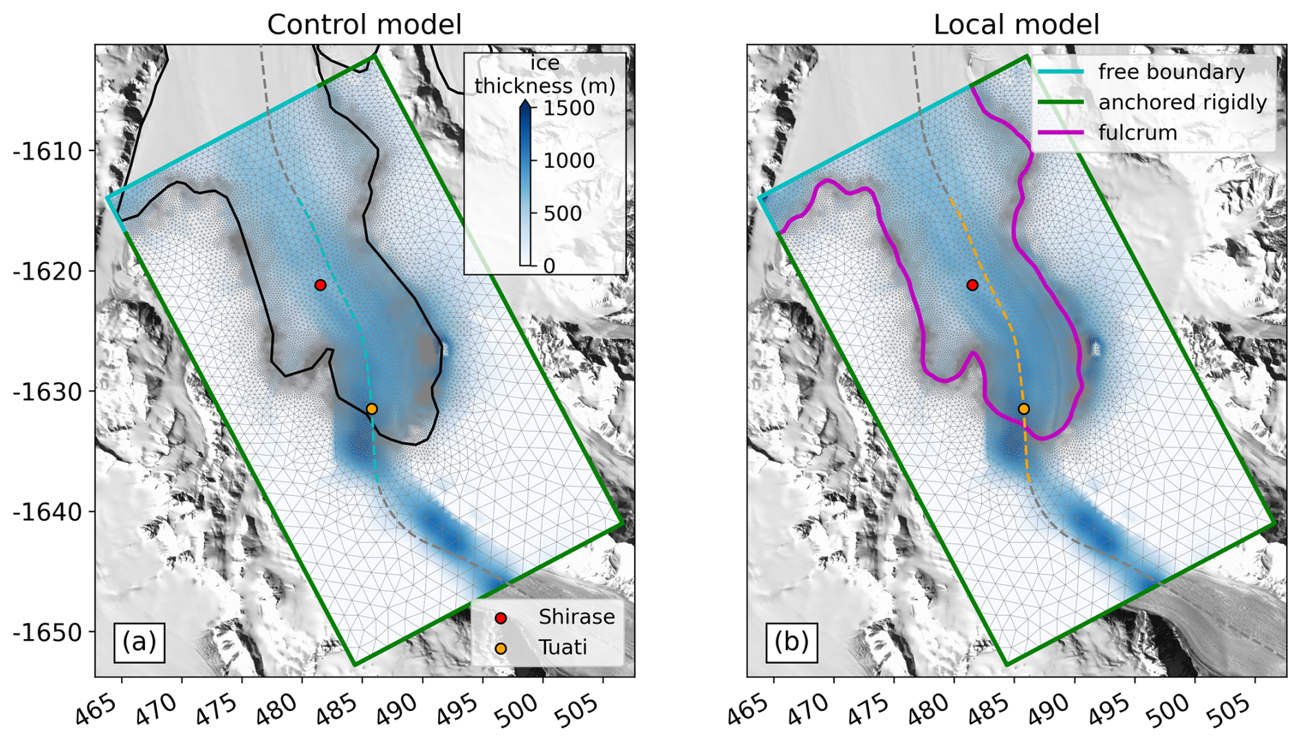
Figure 3 Setups for the control and local models at Priestley Glacier. (a) The control model uses the ASAID grounding line and BedMachine v2 ice thickness. (b) The local model uses a DInSAR-derived grounding line from TerraSAR-X data and ice thickness from freeboard inversion for floating ice. Colored outlines indicate boundary conditions. The finite-element mesh is in the background. The dashed gray line shows the IceBridge flight path (November 2013) with radar data for ice-thickness validation (Appendix A1). Dashed blue and orange lines represent locations of homogeneous model solutions in Fig. 9j and k, respectively.

4 Results

4.1 Tide-model accuracy before and after adjustment

At Priestley Glacier, modeled ocean tides exhibit the highest amplitude variability, reaching ±0.4 m, followed by the IBE, at ±0.15 m, and the load tide, at ±0.05 m (Fig. 4a). The combined effect, referred to as tidal forcing, reaches ±0.6 m. The tides exhibit mainly diurnal characteristics, with a 14 d spring–neap cycle. The correlation between ERA5 reanalysis data and a 59 d pressure record from a local automatic weather station (AWS) at Priestley Glacier is 0.96 (Fig. 4b), indicating high confidence in the IBE correction. We use these time series to predict tidal forcing for the 56 Sentinel-1 SAR data collection times (Fig. 4c and d). The mapped vertical displacements of the 56 SAR acquisitions cover a time interval of more than 1 year and all stages of the tidal oscillation.

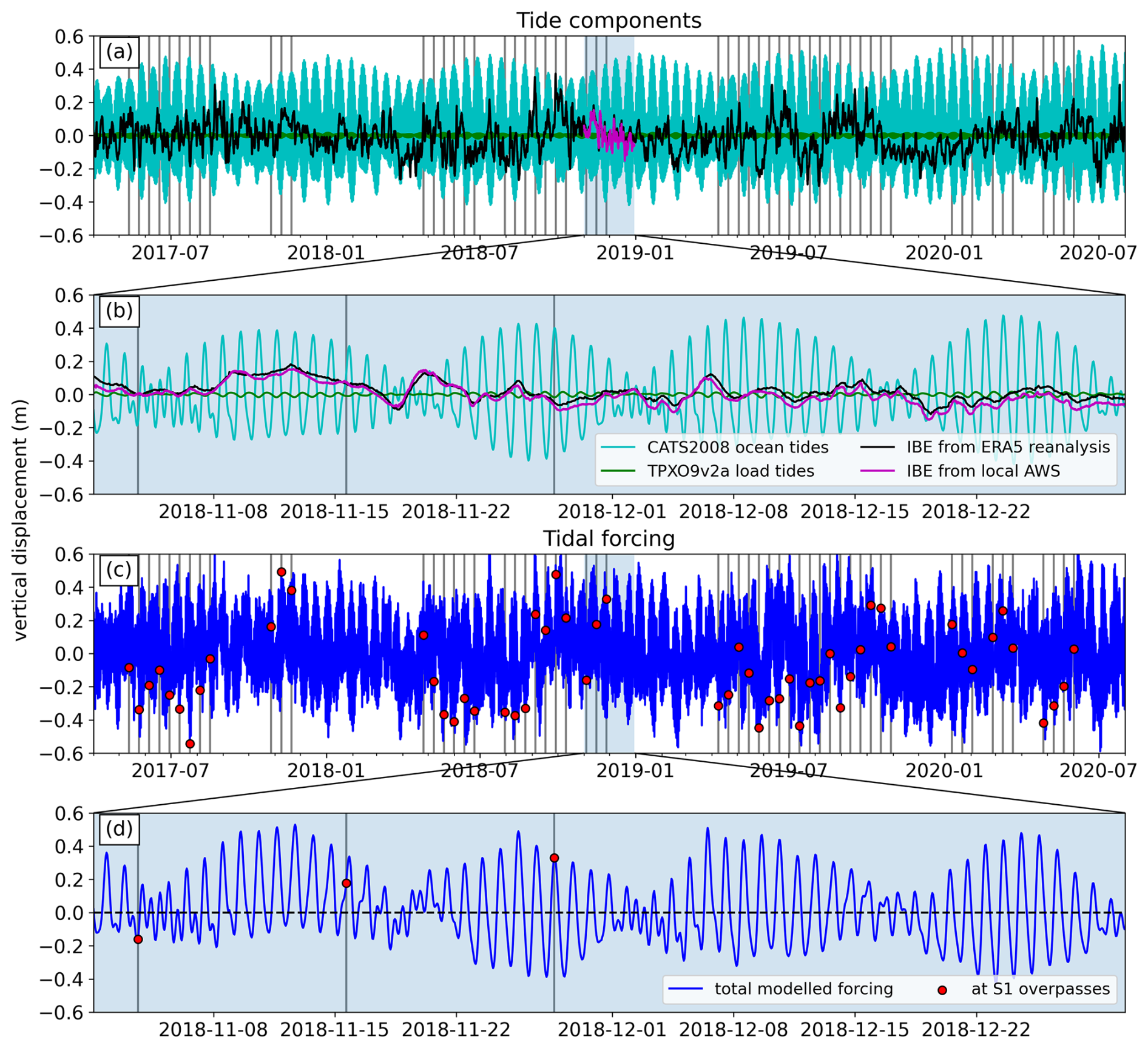
Figure 4 Tidal forcing at Priestley Glacier. (a) Tidal forcing combines the CATS2008 tide model, the TPXO9v2a load model, and the IBE from ERA5 data, compared with an IBE derived from a local AWS. Shaded areas show periods with in situ data for validation. (b) Detailed view of November and December 2018, when AWS and GPS data were collected. (c) Predicted tidal forcing at Sentinel-1 SAR acquisition times. (d) Focused view of November and December 2018. Gray lines indicate SAR acquisition dates; red dots show tidal-forcing values from the model.

Prior to the adjustment with DInSAR observations in the freely floating areas (Fig. 5a), the misfit between the modeled and measured differential tidal displacement is ±0.15 m (Fig. 5b). This is larger than the general accuracy of tide models in Antarctica (±6.5 cm; Stammer et al., 2014). After the adjustment of the modeled tidal forcing (Sect. 3.1.3.), the misfit is reduced to effectively zero, resulting in a match with all measurements (Fig. 5c). The required offsets at the 56 time stamps to achieve this greater accuracy have a mean of 0.04 m and a temporal standard deviation of 0.03 m.

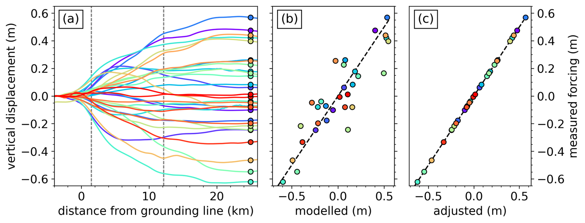
Figure 5 Sentinel-1 DInSAR measurements and tide-model comparison at Priestley Glacier. (a) Vertical displacements along an IceBridge profile in the tidal-flexure zone from 31 DInSAR interferograms. Colored dots show tidal forcing on the ice shelf; dashed gray lines mark the Tuati (flexure zone) and Shirase (floating) GPS stations. (b) Measured vs. modeled tidal forcing (colored dots), with the black dashed line indicating a perfect match. (c) Comparison after adjusting the modeled tidal forcing to align with DInSAR measurements.

The mapping of vertical displacement to individual SAR scenes shows smooth vertical flexure for most stages of the tidal oscillation (Fig. 6). Image quality is, overall, high, with the exception of a narrow band close to the lateral shear zones, which show low coherences throughout the dataset.

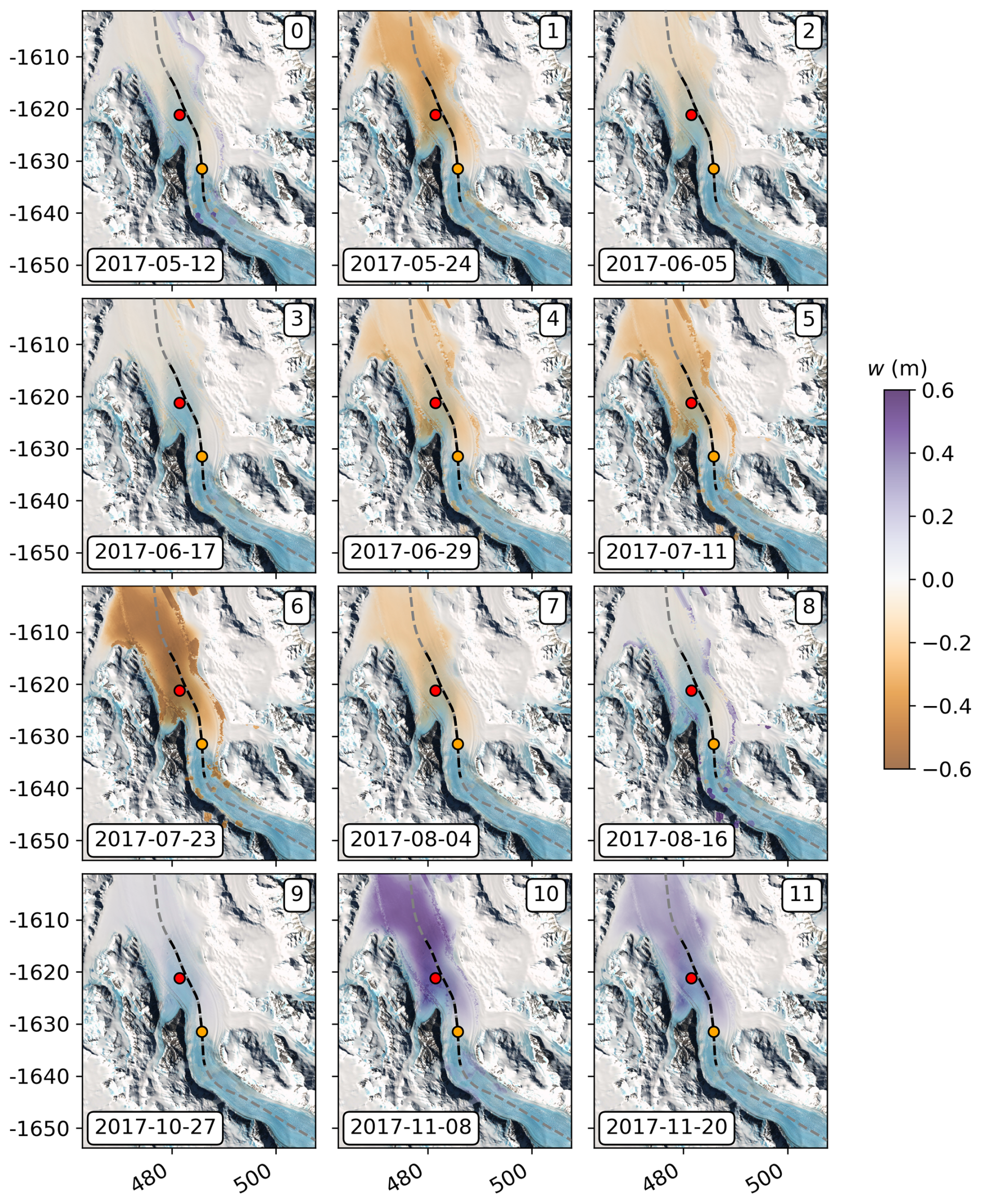
Figure 6 Selection of 12 synthesized vertical displacement maps in the tidal-flexure zone of Priestley Glacier, showing vertical displacement due to ocean tides during SAR data acquisitions in 2017. The dashed line indicates the IceBridge flight path (November 2013). Red and orange dots mark the GPS stations Shirase (freely floating) and Tuati (within the tidal-flexure zone).

With the 56 synthesized displacement maps corresponding to the SAR data acquisition times, we can now generate any desired combination of images. We reassembled the 31 double differences corresponding to the DInSAR combinations to enable a more direct comparison between the measured and mosaicked interferograms. The synthetic interferograms replicate the complex tidal fringes observed in the DInSAR measurements, with discontinuities appearing only outside of the central region of Priestley Glacier (Fig. 7).

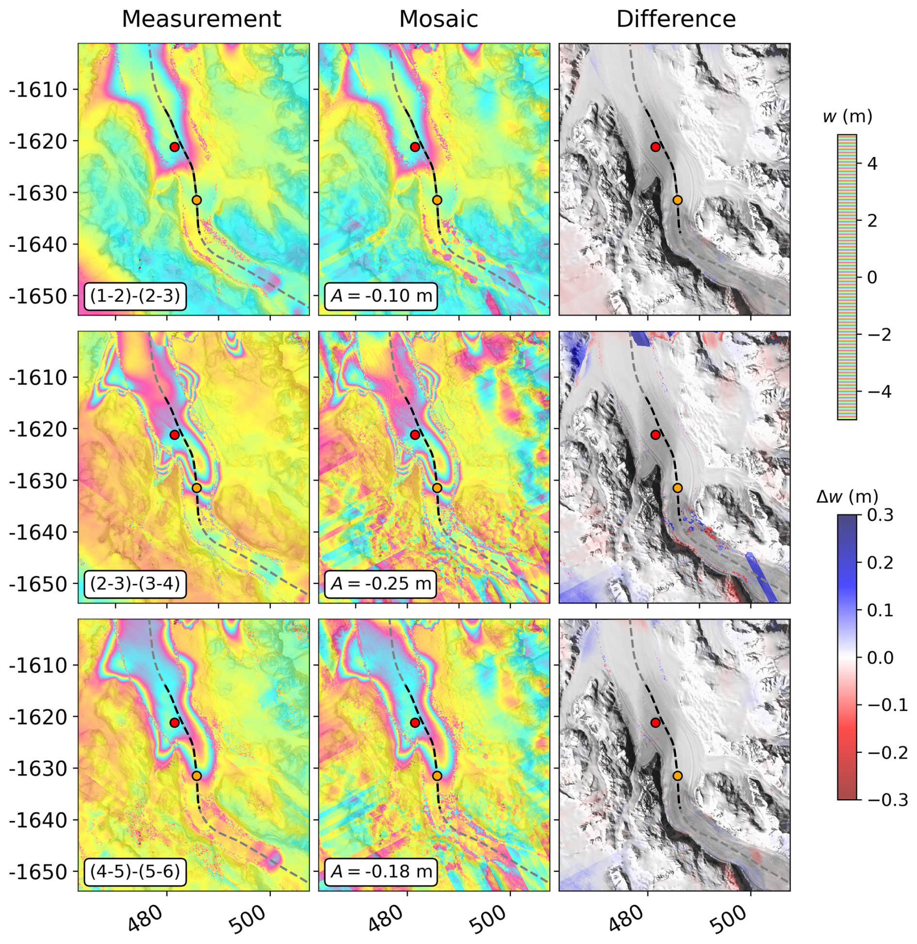
Figure 7 Selection of three measured and mosaicked images from 31 available DInSAR combinations, showing double-differential vertical displacement. The SAR image combination is indicated in the lower left corner. The dashed line marks the IceBridge flight path from November 2013, with red and orange dots showing the locations of the Shirase (freely floating) and Tuati (tidal-flexure zone) GPS stations.

4.2 Effect of ice heterogeneity in lateral shear zones

In the process of DInSAR image mosaicking, we initially used an empirical α-map derived only from all Sentinel-1 DInSAR images. However, alternative α-maps, generated from elastic finite-element model solutions, can also be used to create synthesized vertical displacement maps. This strategy allows us to evaluate the effect of reducing the effective ice stiffness in the shear zone on the tidal-flexure pattern by using modeled α-maps in which the Young's modulus is locally reduced. The goal is to achieve the best possible match between the mosaicked maps and the root-mean-square error (RMSE) between the measured and mosaicked DInSAR images (Fig. 8a).

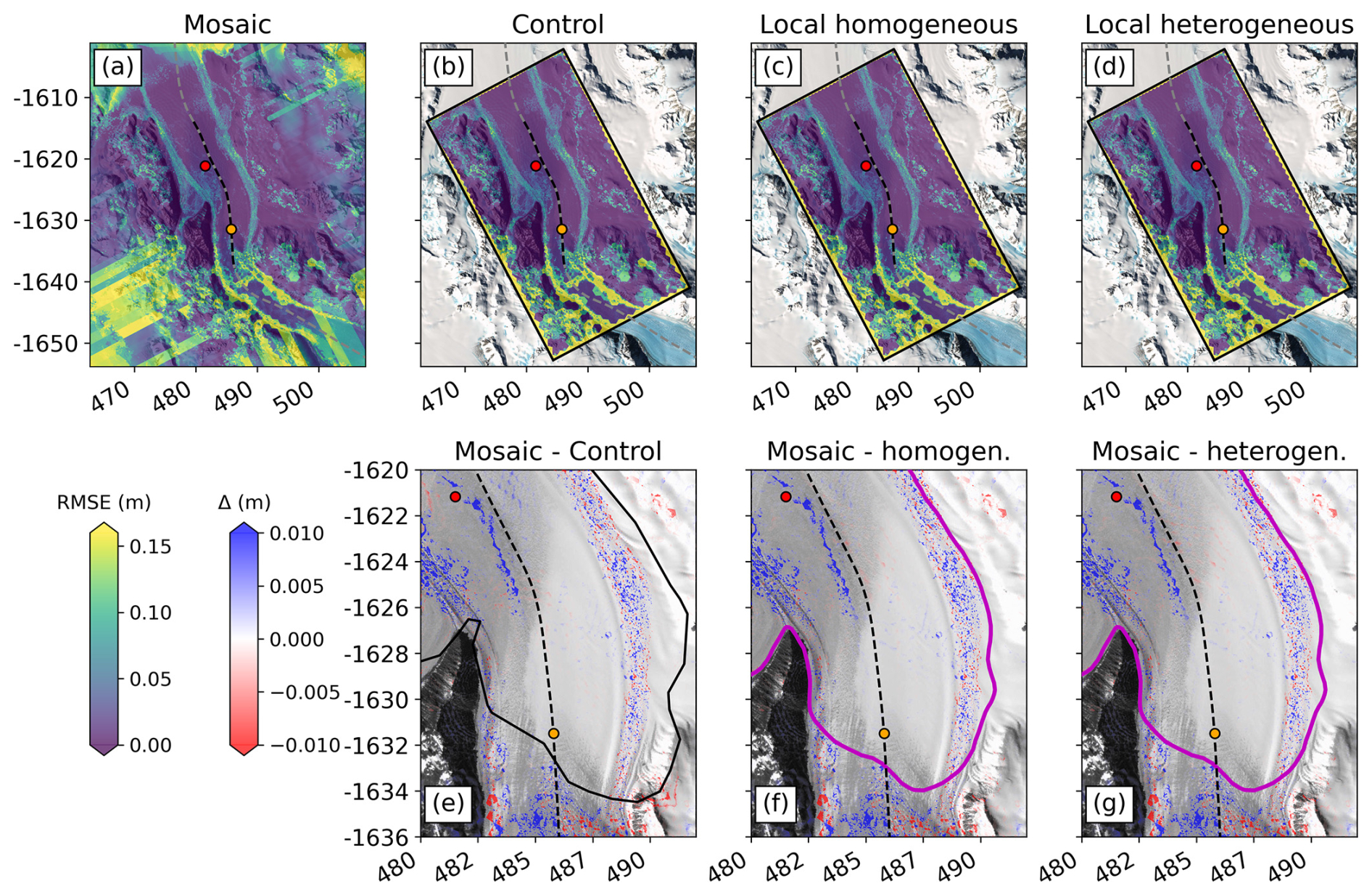
Figure 8 RMSE between 31 DInSAR images measured with Sentinel-1 and least-squares predictions based on various α-maps. (a) Mosaic using an empirically derived α-map from Sentinel-1 data. (b–d) Results from different finite-element model setups. (e–g) Comparison of mosaicked and modeled RMSE, showing that all model setups replicate the mosaic accurately within noise levels (<1 cm).

We tested three distinct finite-element model configurations: (i) the control model, using input data from publicly available datasets; (ii) the local homogeneous model, incorporating ice thickness from the freeboard inversion and DInSAR grounding line but assuming uniform ice properties across the modeling domain; and (iii) the local heterogeneous model, sharing the same input as (ii) but featuring ice stiffness variability, where the Young's modulus is systematically reduced in lateral shear zones. We use the control model as a test for its applicability for a continent-wide assessment, where updated grounding lines and ice thicknesses are not yet available.

All model configurations exhibit minimal RMSE in the central region of the floating ice shelf (Fig. 8b–d), indicating that they align well with the mosaic (Fig. 8e–g), irrespective of the α-map used. This demonstrates that our least-squares adjustment routine, as detailed in Sect. 3.1.4, is effective, regardless of the applied α-map. However, variations within the shear zone are random (Fig. 8e–g) and stem from phase decorrelation in these areas. Therefore, to gain a clearer understanding of the impact of ice stiffness on the tidal-flexure pattern, it is more insightful to directly compare the measured and modeled α-maps, rather than focusing solely on the RMSE between the measured and modeled DInSAR images.

We now compare measured and modeled α-maps (Fig. 9). Both the control model and the local homogeneous model tend to underestimate the measured flexure profile within the first 10 km of the grounding line and overestimate the flexure profile thereafter (Fig. 9j and k). The local model provides a better reproduction of the flexural pattern, compared with the control model, attributed to its more accurate grounding-line location, derived from TerraSAR-X, and its generally thicker ice, which results from the freeboard inversion. This increased thickness helps to account for two-dimensional damping effects (Wild et al., 2018), even at significant distances downstream of the grounding line (12–20 km). The measured flexural pattern is most accurately matched when the Young's modulus in the lateral shear zones is reduced to 20 % (Fig. 9l). Further reducing the Young's modulus to 10 % leads to overestimation of the measured α value.

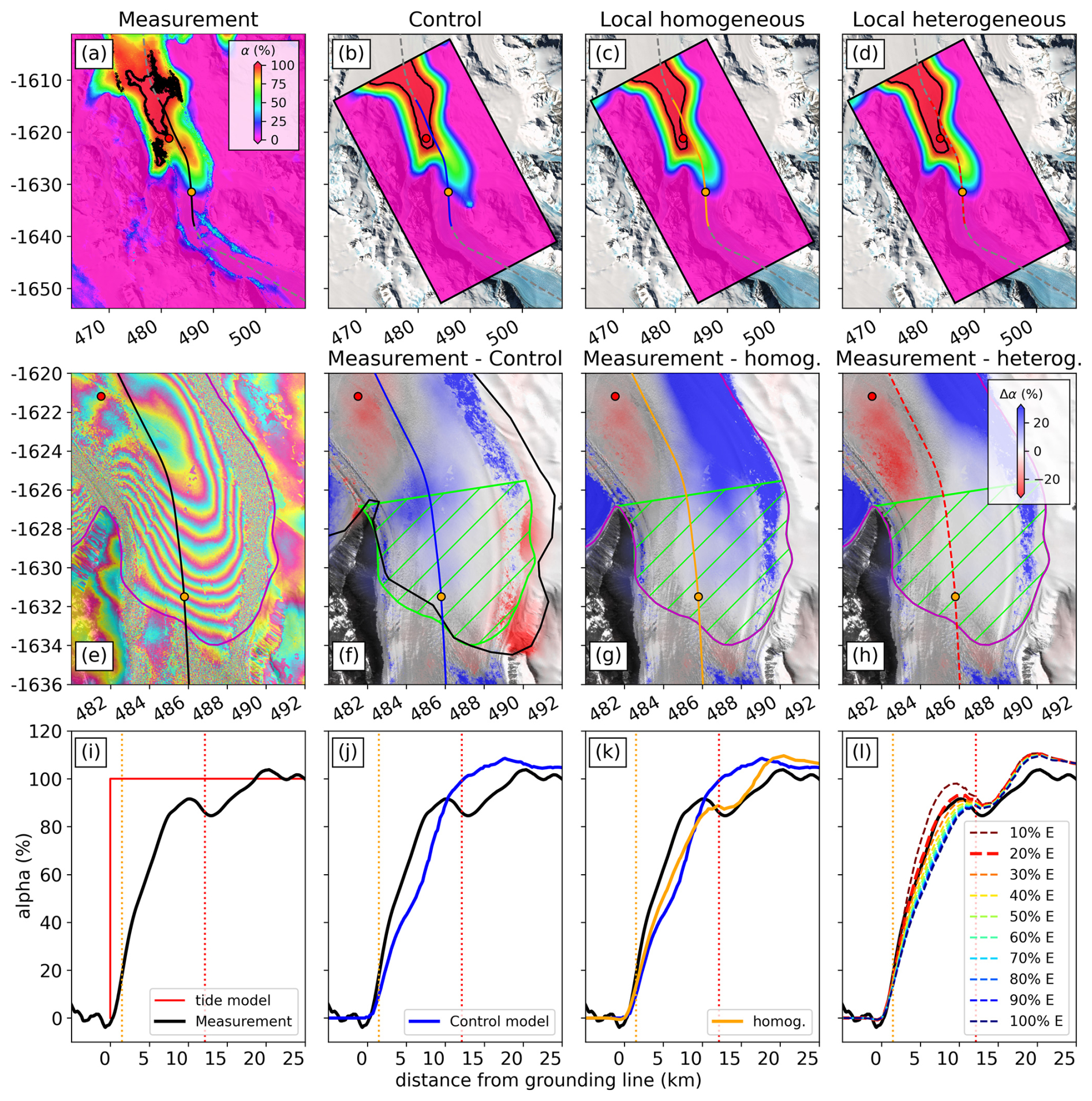
Figure 9 Comparison of percentage tidal displacement determined by various α-maps. (a–d) Tidal displacement percentages: (a) measured from 31 Sentinel-1 interferograms, (b) from the control model, (c) from a homogeneous model, (d) from a heterogeneous model with 20 % effective stiffness in the lateral shear zones. Black contours outline the hydrostatic line, where the ice is in hydrostatic equilibrium, exhibiting full tidal motion (α = 100 %). The dashed gray line marks the IceBridge flight path, indicating flexure curve locations in panels (i–l). (e) Measured tidal fringes in Priestley Glacier's grounding zone, highlighting phase decorrelation in the shear zones. (f–h) Differences between measured and modeled α-maps, with red and orange dots marking GPS receiver locations on the floating and tidal-flexure zones. The green hatched region marks the region analyzed in the scatterplots in Fig. 11. (i–l) Flexure curves, with the heterogeneous model (20 % E in lateral shear zones) closely matching the measured pattern. Dashed lines mark the locations of the Tuati (orange) and Shirase (red) GPS stations.

4.3 Validation with GPS records

We validate our findings using in situ measurements from two GPS sites: Shirase, which is nearly freely floating, and Tuati, located in the tidal-flexure zone. At Shirase, the mean ice-flow speed is 105 m yr⁻¹, while at Tuati it is 131 m yr⁻¹. These speeds are consistent with TerraSAR-X-derived measurements of 96 and 132 m yr⁻¹, respectively. To isolate the vertical tidal signal, we remove linear trends of −0.81 m yr⁻¹ at Shirase and −2.44 m yr⁻¹ at Tuati from the GPS elevation records. We then compare the resulting anomalies with tidal forcing predicted using various α-values from different models (Fig. 10).

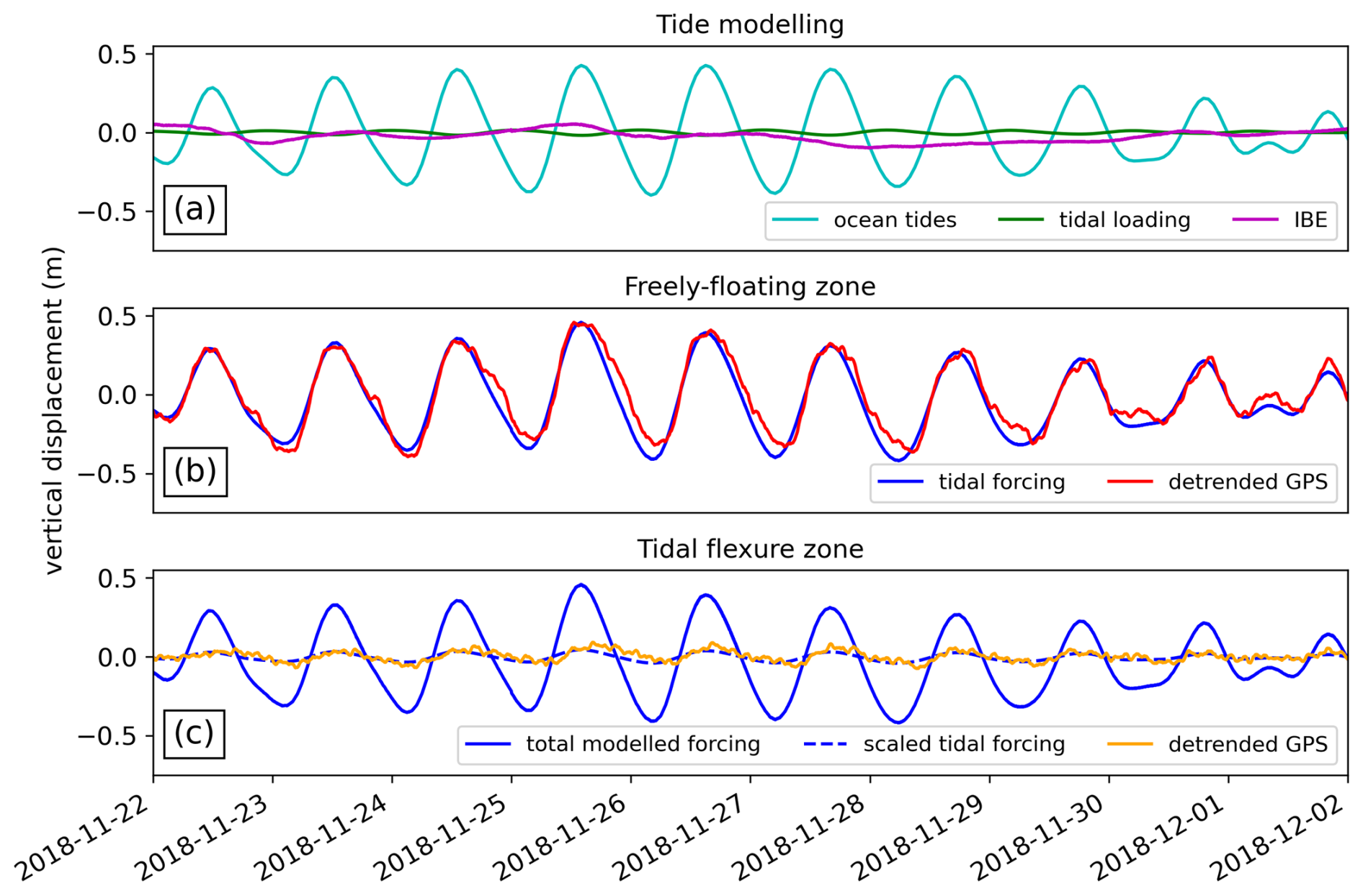
Figure 10 Example of improved tide-model output over one neap–spring–neap tidal cycle, achieved through linear scaling with the tide–deflection ratio from the control model. (a) Components of tidal forcing. (b, c) Tide modeling (b) accurately predicts measured vertical displacement where ice is freely floating but (c) neglects the damping effect of ice dynamics in the tidal-flexure zone if unscaled. The locations of the two GPS receivers are shown in Fig. 9.

The measured α-value for the Shirase GPS site is 89.6 %, which is overestimated by all model setups (control model: 105.8 %; local homogeneous: 101.5 %; local heterogeneous: 104.0 %). For Tuati, the measured α-value is 17.5 %, with the best match provided by the local heterogeneous model (control model: 9.8 %; local homogeneous: 13.2 %; local heterogeneous: 16.2 %).

Using these α-values, we linearly scale the previously derived tidal forcing to predict vertical tidal motion at the GPS locations. Including tidal loading and the IBE reduces the RMSE between the unscaled tidal forcing and the freely floating Shirase GPS measurements from 0.076 to 0.067 m. Scaling with the measured α-value improves the RMSE to 0.064 m. However, the modeled α-values slightly worsen the fit for Shirase (control model: 0.071 m; local homogeneous: 0.068 m; local heterogeneous: 0.07 m).

The benefits of using an α-map are more pronounced in the spatially extended tidal-flexure zone. The RMSE between the unscaled tidal forcing and the Tuati record is 0.182 m. Scaling with the measured α-value of 17.5 % improves the fit to 0.03 m (or by 84 %). The various modeled α-maps offer slightly better fits (control model: 0.027 m; local homogeneous: 0.027 m; local heterogeneous: 0.029 m). Therefore, as expected, any α-value scaling improves the fit between observed and predicted tidal displacements. The differences between using the α-values from our three model scenarios are small and show only comparatively little variability across the different model scenarios. This means that the locations of Shirase and Tuati are not particularly sensitive to the modeling choices, as is also evident in Fig. 9f–h. However, differences between the different model scenarios are more pronounced when evaluated across the entire flexure zone, as opposed to along the central flowline only.

In the tidal-flexure zone (green hatched region in Fig. 9f–h), local heterogeneous models with a Young's modulus ranging from 30 % to 100 % consistently underestimate the satellite-derived percentage of tidal displacement. The optimal fit is obtained with a 20 % Young's modulus. A 10 % Young's modulus tends to overestimate the tidal flexure, particularly for high α-values near the hydrostatic line (Fig. 11). The RMSE for the homogeneous case is 14.8 %, while that for the best heterogeneous case is 10 %, representing an improvement of 33 %. Further reducing the Young's modulus from 20 % of its reference value to 10 % increases the mismatch again, raising the RMSE to 10.4 %.

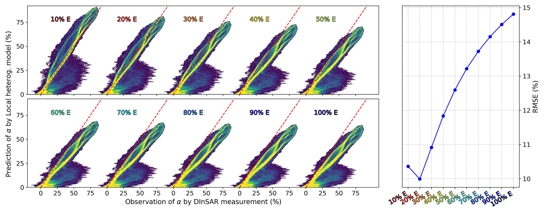
Figure 11 Scatterplots comparing measured and modeled α-maps from the local heterogeneous model of the tidal-flexure zone near Priestley Glacier's grounding line. Point density is color-coded, with yellow denoting high density. The dashed red line represents a perfect match. The heterogeneous model, using a 20 % Young's modulus in the shear zone, aligns best with measured values. The RMSE for each scatterplot is minimal for 20 % E and maximal for the homogeneous case (100 % E).

5 Discussion

5.1 Hypothesis evaluation: ice stiffness reduction in shear zones

Our results indicate that heterogeneous flexure models provide a better fit to DInSAR observations than their homogeneous counterparts. This supports the idea that satellite interferometry is sensitive to spatial variations in ice stiffness, particularly across shear zones. However, this interpretation depends on the choice of the reference Young's modulus, which we set to E = 1.6 GPa. To explore the sensitivity of our findings to this assumption, we conducted additional simulations using the homogeneous model. We find that lowering the homogeneous Young's modulus to E = 1.0 GPa yields a fit to the DInSAR measurements comparable to that of the best-fit heterogeneous model, which assumes E = 1.6 GPa with a 20 % reduction across shear zones (Fig. 12). This nonuniqueness highlights the importance of better constraining field-derived estimates of the effective Young's modulus.

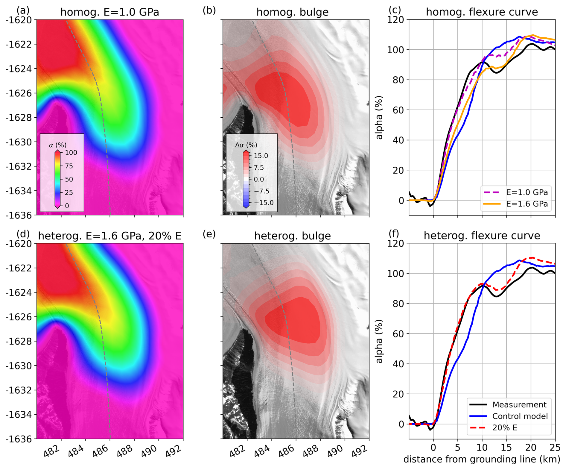
Figure 12 Comparison between the best homogeneous and best heterogeneous flexure-model solutions. (a) Elastic flexure for a homogeneous Young's modulus of E = 1.0 GPa. (b) Difference relative to the homogeneous reference case of E = 1.6 GPa. (c) Flexure curves for both homogeneous cases, compared with the DInSAR measurements and the control model. (d) Elastic flexure for a heterogeneous ice stiffness model with E = 1.6 GPa and a 20 % reduction in the lateral shear zones. (e) Difference between the best heterogeneous case and the homogeneous reference (E = 1.6 GPa). (f) Best-fit heterogeneous flexure curve, compared with satellite observations and the control model.

The reference value of E = 1.6 GPa is based on previous tiltmeter measurements from a relatively simple setting on the southern McMurdo Ice Shelf, which features a thick firn layer and limited lateral variability (Wild et al., 2017). In contrast, Priestley Glacier contains well-defined shear zones, consists largely of blue ice, and originates from the polar plateau, where ice temperatures are significantly colder. Given these differences, we expect Priestley Glacier ice to be inherently stiffer than that of the southern McMurdo Ice Shelf. For this reason, we retain E = 1.6 GPa as the reference value for our heterogeneous experiments and do not adopt the reduced homogeneous value as a new baseline.

This result is reminiscent of findings from Darwin Glacier, where tiltmeter data indicated a Young's modulus of E = 1.0 GPa (Wild et al., 2019). Like Priestley Glacier, Darwin Glacier exhibits a pronounced lateral shear zone and is composed predominantly of blue ice. These similarities raise questions about the appropriateness of using a reduced Young's modulus in such settings, where colder ice temperatures and structural complexity should lead to higher stiffness.

5.2 Elastic weakening in shear zones: contradictions and interpretations

In Wild et al. (2019), we identified a narrow band of relatively larger model misfits stretching from Darwin Glacier's shear margin to the freely floating ice shelf. These discrepancies were attributed to the microscopic process of ice anisotropy, to explain the observed macroscopic response and account for the glacial heterogeneity within the embayment. In the present study, we attempted to replicate a similar signal within the shear zone of Priestley Glacier using Sentinel-1 data. However, phase decorrelation in the shear zone impeded a direct enhancement of the model fit in these lateral regions.

However, the core issue is that we observe apparent elastic weakening within shear zones, which stands in contrast to laboratory measurements indicating that ice anisotropy has only a minimal effect on the elastic properties of glacier ice (Lutz et al., 2022; Rathmann et al., 2022). This suggests that attributing reductions in Young's modulus within shear zones to ice fabric is not physically justified. Our efforts also rely on isotropic material assumptions, which do not align with natural ice masses (Jacka and Budd, 1989). In regions characterized by simple shear, such as the lateral shear zones of fast-flowing outlet glaciers, there is a notable transition from initially isotropic to anisotropic ice (Thomas et al., 2021). This transformation results in a robust fabric aligned perpendicular to the shear plane, primarily due to the basal glide deformation of individual crystals. As grain rotation and dynamic recrystallization take place within the polycrystal, a preferred orientation fabric emerges, leading to bulk softening of ice stiffness. In polycrystalline shear zone ice with well-developed fabrics, the enhancement of ice flow can be up to 10 times greater than in the isotropic case (Hudleston, 2015). This becomes significant in regions where fast-flowing glaciers are constrained along their margins, leading to the disappearance of basal drag, and shear stresses from lateral boundaries become the sole determinant of effective strength to resist grounding-line discharge (Gudmundsson, 2013).

More broadly, the contradictions between field- and laboratory-derived properties call into question the appropriateness of using Young's modulus as a bulk tuning parameter to represent the combined effects of fabric, temperature, and damage. While ice fabric has limited influence on elastic properties, it significantly affects the viscous behavior of glacier ice. Given that tidal flexure is fundamentally a viscoelastic process, it would be more physically consistent to vary ice viscosity, rather than elasticity, within shear zones when tuning models to match observations. Nevertheless, because our analysis is based on comparisons of modeled and observed α-maps, which are temporally averaged and thus largely filter out transient viscoelastic signals, we sidestep the need to explicitly implement a viscoelastic model in this study.

This α-map based approach is only feasible because a long time series of Sentinel-1 data is available, capturing the full tidal cycle and enabling a reliable temporal average of the flexural response. As publicly accessible SAR satellite data become more abundant, we anticipate significant progress in our understanding of shear-zone weakening. This advancement will enhance the applicability of the methods outlined in this study, potentially informing the next generation of ice-sheet models with improved maps of spatially heterogeneous ice properties along Antarctica's grounding line.

5.3 Limitations and opportunities for improving shear-zone characterization

Caveats of our method are the reliance on synthesizing “single-tide” displacement maps and limited interferometric coherence for resolving fringes across the shear zone. These, in turn, hamper our capacity to unequivocally distinguish between potential mechanisms of shear-zone weakening – such as anisotropy, shear heating (Perol and Rice, 2015), fracturing (Albrecht and Levermann, 2014), or nonlinear viscous effects governed by Glen's flow law under tidal loading (Rosier and Gudmundsson, 2018). To definitively link the observed weakening in the shear zone of Priestley Glacier to the macroscopic influence of ice-crystal anisotropy, more in situ data are required. These data should not only capture “single-tide” vertical flexure but also resolve fringes across the shear zone, particularly where Sentinel-1 data lose sufficient coherence. It remains unclear whether the phase decorrelation observed in the shear zone of Priestley Glacier stems from intrinsic differences in setting, compared with Darwin Glacier, or if it is related to the use of Sentinel-1 data, which differ from the TerraSAR-X data used in our previous study. Despite this limitation, we successfully matched tidal flexure in the central areas of Priestley Glacier, providing evidence for shear-zone weakening and its macroscopic influence on the flexural pattern.

Terrestrial radar interferometry, as applied by Drews et al. (2021a) to the upstream section of Priestley Glacier, could fill this data gap due to its significantly higher temporal resolution (minutes to hours) compared with satellite SAR data (days to weeks). With tidal fringes extending across the shear zone, it would be possible to better constrain viscoelastic models in key regions affecting Priestley Glacier's resistance to vertical displacement, rather than using its central part as a proxy for processes occurring along its sides.

5.4 Justification for using an elastic approximation

The RMSE provides a useful measure of the absolute fit between the modeled tidal forcing and GPS records. However, it does not offer information about the timing of tidal oscillations at the two sites. To address this, we examine the correlation between unscaled tidal forcing and the GPS records. For Shirase, including load tides and the IBE improves the correlation from 0.92 to 0.94. For Tuati, the correlation increases from 0.62 to 0.66. The difference in correlation between the two GPS sites, about 0.3, suggests varying timing of tidal oscillations, which we attribute to viscoelastic effects. In an ideal elastic scenario, tidal deformation would occur instantaneously, leading to consistent correlations across the tidal-flexure zone, though with a reduced tidal amplitude through flexural damping.

Figure 13 illustrates the effect of introducing a synthetic time shift on the correlation between tidal forcing and GPS measurements. Applying a 0.37 h shift to the unscaled tidal forcing improves the correlation with the Shirase GPS measurements from 0.94 to 0.95. This minor improvement supports the assumption of hydrostatic equilibrium at the freely floating GPS site. In contrast, applying a 1.3 h time shift enhances the correlation between the flexure-zone GPS data and the tide-model output from 0.66 to 0.72, suggesting that viscoelastic time delays occur between the two GPS sites. Although estimating ice viscosity for a more precise fit is theoretically feasible, the elastic model used in this study achieves an 84 % improvement, compared with a tide model excluding tidal flexure, and provides a substantial enhancement. Further exploration of viscoelastic modeling is planned for future research.

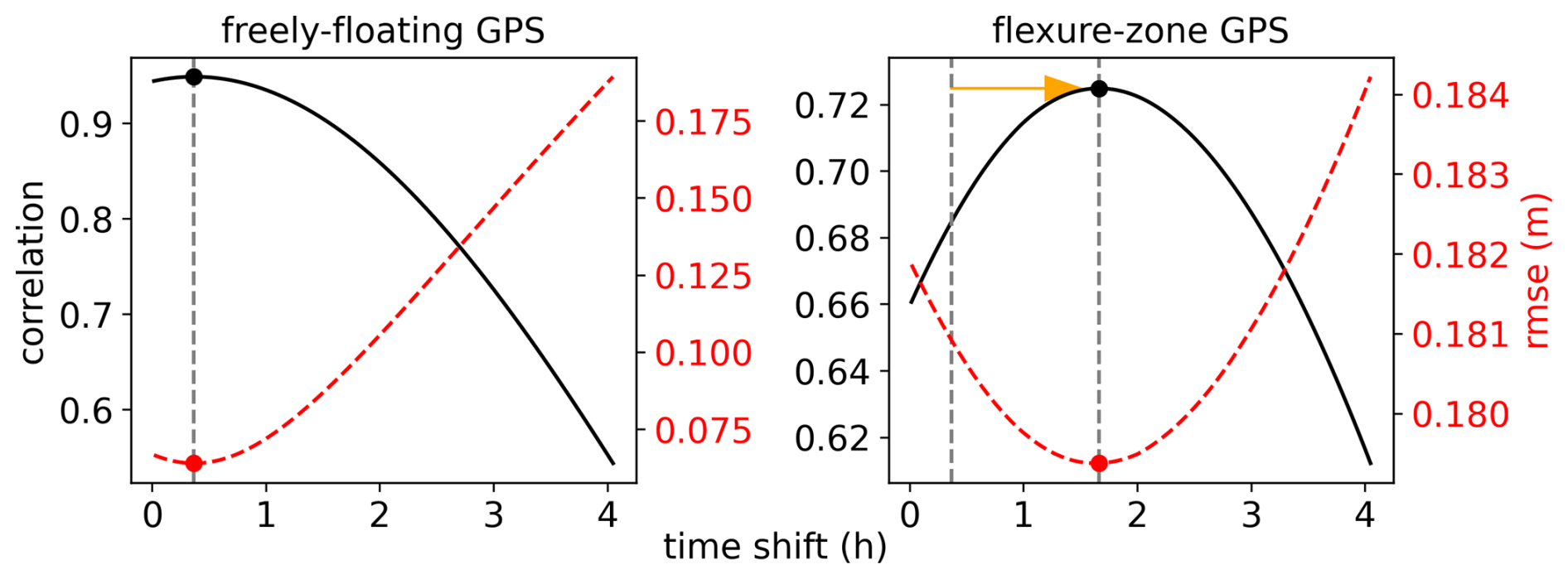
Figure 13 Correlations and associated RMSE between GPS measurements and tide-model output as a function of a synthetic time shift. The length of the orange arrow corresponds to a 1.3 h time delay that we largely attribute to viscoelastic time delays in the flexural response between the two GPS sites.

To approximate tidal flexure with an elastic model, significant tidal amplitudes during SAR image acquisition are crucial to minimize viscoelastic time delays (Wild et al., 2017). Instead of selecting individual DInSAR images for large tidal amplitudes, we reduce viscoelastic effects by computing a percentage tidal displacement field over all 31 Sentinel-1 DInSAR images (α-map; Han and Lee, 2014; Wild et al., 2019). This averaging approach also addresses geometric effects from horizontal surface motion around a neutrally deforming layer at the center of the ice shelf (Video S1 in the Supplement; Rack et al., 2017; Wild et al., 2018). Generating an α-map assumes minimal tidal grounding-line migration, as observed at Priestley Glacier, where high-temporal resolution terrestrial radar interferometry indicates horizontal grounding-line migration well below the scale of one ice thickness (Drews et al., 2021a).

5.5 Asymmetric tides and potential role of ephemeral re-grounding

Our GPS data show an asymmetric ocean tide, with a noticeably steeper rising tide compared with the falling tide (Fig. 10b). This asymmetry is not captured by the tide model, which predicts a more balanced symmetric tidal oscillation. There are a couple of potential explanations for this discrepancy: (1) preferential propagation of the tidal wave, which might enhance tidal inflow into the sub-ice-shelf cavity more than the outflow during the falling tide, or (2) transient re-grounding of the ice shelf at low tide. The latter has been suggested by Drews et al. (2021a) and could be linked to upstream flexure opposing the direction of the falling tide. This opposing flexure may suggest the formation of a temporary fulcrum offshore of the grounding line, potentially aligning with undulations in the bathymetry. However, our tidal-flexure model currently does not account for the shape of the offshore bathymetry, preventing us from evaluating the effects of transient re-grounding. Although it would be theoretically possible to incorporate the bathymetry as an elastically deforming boundary condition – similar to the bed beneath grounded ice in the current model setup – the limited availability of bathymetric data in the tidal-flexure zone complicates this modeling effort (Appendix A2).

6 Conclusions

This study highlights the importance of accounting for ice heterogeneity and tidal flexure in modeling the dynamics of Antarctic outlet glaciers. By integrating Sentinel-1 DInSAR data with tidal-flexure models, we demonstrated that reducing ice stiffness in lateral shear zones significantly improves the accuracy of vertical displacement predictions, particularly along the grounding line. Questions remain regarding the choice of the reference Young's modulus. In our heterogeneous experiments, we use E =  1.6 GPa, while in the homogeneous experiments we adopt E =  1.0 GPa, providing an alternative and equally valid explanation for the observed behavior. This highlights the need for better constraints on field-derived estimates of the effective Young's modulus. Nonetheless, we emphasize the broader utility of DInSAR beyond its conventional role in delineating grounding lines of ice shelves to map spatially variable ice properties – a first step toward mapping ice rheology along the Antarctic coastline to inform ice-sheet models.

Incorporating DInSAR in large-scale ice-sheet monitoring not only enhances our understanding of glacial dynamics but also provides a critical tool for mapping the mechanical properties of ice, essential for future studies on ice rheology and deformation. Expanding this approach to other Antarctic outlet glaciers, combined with the increasing availability of satellite data, will further refine our knowledge of ice heterogeneity and its impact on glacier flow, potentially transforming how we predict ice-sheet responses to a changing climate.

Appendix A

A1 Ice-thickness validation with airborne radar

Figure A1 illustrates a radar transect along an IceBridge flight path acquired in November 2013 (Paden et al., 2010), covering Priestley Glacier as it merges with the Nansen Ice Shelf. The REMA surface elevation data closely match the airborne measurements from IceBridge. However, discrepancies are more pronounced in the ice base measurements. Upstream of the grounding line, marked by a distinct reduction in basal reflectivity on the IceBridge radargram (black line in Fig. A1), the freeboard inversion method significantly overestimates ice thickness by several hundred meters. Consequently, the BedMachine ice thickness product is employed for both the control and local models in this region.

In contrast, downstream of the grounding line, the freeboard inversion ice thickness estimates align well with the airborne measurements. Here, the ice thickness decreases from approximately 1000 m at the grounding line to about 250 m near the ice-shelf front, consistent with the hydrostatic equilibrium assumed in this portion of the Nansen Ice Shelf.

A2 Sensitivity tests

Our analysis indicates that the Young's modulus in the shear zones is reduced by a factor of 5. To assess whether this effect stems from our model assumptions or represents a robust feature of the data, we performed a number of model experiments. Specifically, we investigated how varying the homogeneous Young's modulus and decreasing the foundation's spring stiffness beneath the grounded ice influence the modeled elastic response in our idealized setup. This setup assumes an idealized ice thickness and a grounding-line embayment resembling the geometry of Priestley Glacier, as described in Sect. 2.1.

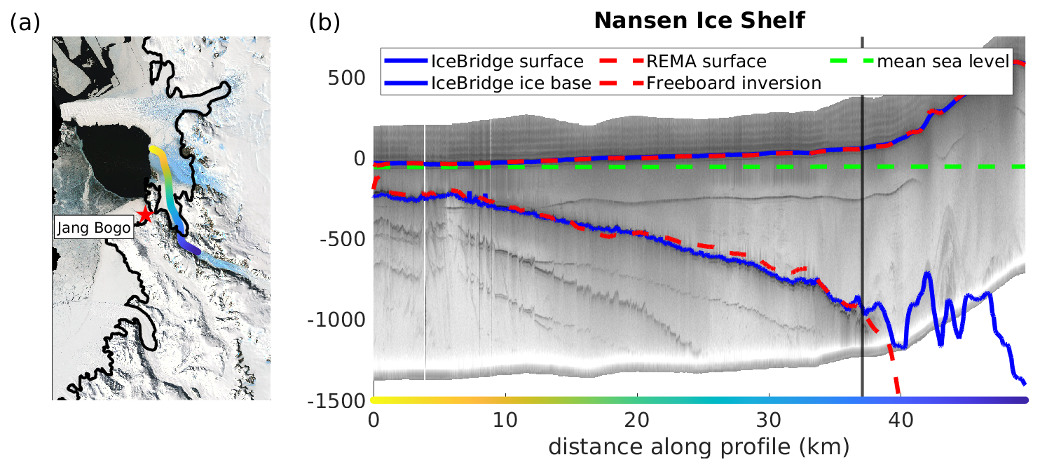
Figure A1 IceBridge radar profile, following the IceBridge flight path shown in panel (a). Panel (b) presents the airborne measurements of ice surface and ice base elevation (blue lines). REMA data indicate the ice surface elevation, while inversion of the freeboard is used to determine the ice base depth (dashed red lines). Mean sea level is referenced against the EIGEN-6c4 geoid (dashed green line). The approximate location of the grounding line is marked in black.

We systematically varied the homogeneous Young's modulus around its reference value of 100 % E = 1.6 GPa and found that reducing the Young's modulus, i.e., softening of the ice, steepens the modeled tidal-flexure curve for a given tidal amplitude of A = −1 m. This steepening is most pronounced at the floating sections of a grounding-line embayment (Fig. A2a) and moves the offshore inflection point, where tidal flexure over-shoots the applied forcing closer to the grounding line (Fig. A2b).

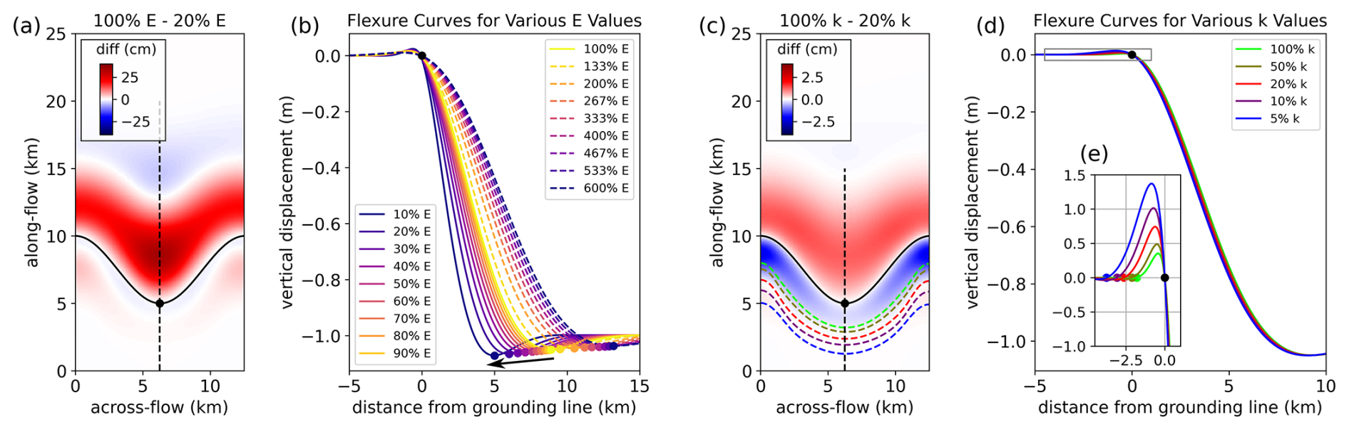
Figure A2 Sensitivity of tidal flexure to varying Young's modulus and bed stiffness. (a, c) Range of tidal flexure for Young's modulus/bed stiffness from 20 % to 100 % as a function of grounding-line geometry. (b, d) Tidal-flexure curves for both increasing and decreasing reference values. (e) Enlargement of the upstream bulge area, showing vertical displacement in centimeters along the y axis.

Reducing the foundation stiffness to 5 % of the reference value (k = 5 MPa m⁻¹) increases the flexure on both the floating and grounded portions of the ice. The differences between 100 % k and 20 % k are most pronounced at the grounded sections of adjacent grounding-line protrusions and least pronounced along the glacier centerline (Fig. A2c). Along the centerline, the modeled flexure curve shows a mean range of 0.3 ± 0.3 cm on the grounded portion and 1.6 ± 1.1 cm on the floating portion, measured from the grounding line to 10 km in the along-flow direction (Fig. A2d). This corresponds to a maximum of 2 %–3 % of the applied 1 m tidal forcing, which is significantly smaller than the 10 % bulge observed between the heterogeneous and homogeneous cases.

Interestingly, the inland extent of the grounding-line bump (Fig. A2e) is also influenced by the grounding-line geometry, with protrusions exhibiting a greater inland reach than the glacier centerline (Fig. A2c). This occurs because grounding-line protrusions have more surrounding floating ice available to induce flexure on the grounded part, compared with a grounding-line embayment.