How well do the regional atmospheric and oceanic models describe the Antarctic sea ice albedo?

We assessed how well regional climate models (HCLIM, MAR, RACMO), ocean models (MetROMS-UHel, NEMO), and ERA5 reanalysis simulate Antarctic sea ice albedo, snow, and ice thickness, using in situ data from field campaigns (ISPOL, Weddell Sea, in December 2004, and Marsden, McMurdo Sound, in November 2022) and satellite observations. The simulations performed were obtained with albedo parameterisations that greatly differed in complexity. While simple albedo parameterisations performed well in specific conditions applying ad hoc tuning (for instance, RACMO reproducing the Marsden albedo time series the most accurately), they struggled in simulating key processes. The most advanced albedo scheme applied in MetROMS-UHel produced the best overall results (including the diurnal albedo variability) when compared with ISPOL albedo time series and the observed albedo distribution from CLARA-A3 satellite products. In drier sea ice regions like the Ross Sea, the key issues affecting the accuracy of albedo models are the treatment of fractional snow cover and the snow albedo dependence on snow depth. Higher-resolution models do not necessarily outperform lower-resolution models if small-scale spatial variations in sea ice concentration, snow patchiness, and blowing snow are not accounted for. We believe that integrating the most sophisticated albedo schemes into regional climate or ocean models represents a major step forward in accurately simulating surface energy processes. Moreover, high-resolution topography and sea ice concentrations would be crucial to simulate complex coastal areas such as the Marsden campaign site.

1 Introduction

The Antarctic sea ice zone covers approximately 19×10⁶ km² in winter and 3.5×10⁶ km² in summer. Sea ice plays a crucial role in the polar climate due to its high albedo compared to the open ocean, significantly influencing the surface energy budget and, consequently, the mass and heat balance of the sea ice. This can initiate a positive feedback loop, where the loss of sea ice and snow cover reduces albedo, further increasing surface temperatures and accelerating the melt and increasing sea ice loss. This positive surface albedo feedback has been shown to contribute to Arctic amplification in both models and observations (Previdi et al., 2021, and references therein) but is less reported in the Antarctic (Casado et al., 2023).

Accurately representing the properties of sea ice, such as the albedo, ice and snow thickness, and their interactions with the atmosphere and ocean is crucial for reliable predictions in polar regions. These properties of sea ice can vary significantly. Sea ice consists of ice floes of varying thickness, typically covered by snow, and is often fragmented by cracks, leads, and polynyas. The surface albedo of sea ice depends on snow and ice characteristics and can range widely – from 0.9 for dry fresh snow to 0.4 for melting bare ice – but the spatial average albedo is highly affected by the fraction of open water, as it has an albedo of 0.06 (Warren, 1982; Perovich and Gow, 1996; Pirazzini, 2004; Light et al., 2022). The albedo also depends on planetary and atmospheric factors, such as the solar zenith angle and cloud cover.

Simple parameterisation schemes for sea ice are traditionally employed in regional atmospheric climate model applications. This is the case for the models used in this study: HCLIM (Belušić et al., 2020), MAR (Gallée and Schayes, 1994), and RACMO (van Dalum et al., 2024). In these models, sea ice concentration is prescribed, while sea ice thickness is either fixed (as in RACMO) or thermodynamically evolving (HCLIM, MAR), while neglecting the dynamical processes. In ocean modelling, more advanced dynamic–thermodynamic sea ice models are often applied. Examples of these include NEMO (Nucleus for European Modelling of the Ocean, Madec and the NEMO System Team, 2024) with the sea ice engine SI³ (Sea Ice modelling Integrated Initiative, Vancoppenolle et al., 2023) and ROMS (Regional Ocean Modelling System, Shchepetkin and McWilliams, 2005) coupled with the sea ice model CICE (Community Ice CodE, Hunke et al., 2022) by Debernard et al. (2017), Naughten et al. (2017), and Äijälä et al. (2025).

Both the regional atmospheric climate models and the regional ocean models rely on sea ice albedo parameterisation recommendations, such as those given in Ebert and Curry (1993), Perovich and Gow (1996), Curry et al. (2001), Pirazzini (2004), Liu et al. (2007), and Briegleb et al. (2007). Sea ice albedo is typically parameterised as a function of one or more variables, including air temperature, skin temperature, snow/ice type, snow grain size, snow depth/density, sea ice thickness, cloud cover fraction, and solar zenith angle. The complexity of these parameterisations varies depending on the intended application of the model. In the simplest cases, sea ice albedo is presented as climatological mean values, as in ERA5 (Hersbach et al., 2020) and RACMO, which use Ebert and Curry (1993) parameterisations. When more sophisticated radiative transfer schemes are applied, albedo is calculated based on the inherent optical properties of the surface (e.g. snow model CROCUS used in MAR, Brun et al., 1992).

Curry et al. (2001) and Liu et al. (2007) pointed out, that most climate modellers have justified using simple snow/ice albedo parameterisations because of the lack of observations against which to evaluate them. Indeed, detailed sea-ice-albedo-specific studies, which compare both observations and models, are rare. Recently, Jäkel et al. (2024) tested the coupled Arctic atmosphere–ocean–sea ice model HIRHAM–NAOSIM in the Arctic against MOSAiC campaign in situ observations, aircraft measurements, and satellite images. They found large (>0.1) discrepancies between albedo observations and models during the melt season and concluded that the surface-type parameterisation contributes significantly to the bias in albedo. Furthermore, the ERA5 sea ice albedo, or more exactly, the sea ice albedo of the Integrated Forecasting System (IFS) model of the European Centre for Medium-Range Weather Forecasts (ECMWF), has been identified as a limitation by several studies over the Arctic region (Pohl et al., 2020; Müller et al., 2024; Batrak et al., 2024). Batrak et al. (2024) investigated the albedo of sea ice in ERA5 and the Copernicus Arctic Regional Reanalysis (CARRA) dataset and found springtime albedo errors of around 0.06 and 0.14 respectively, computed against the CLARA-A2 satellite retrieval product (Karlsson et al., 2017). Therefore, both reanalysis datasets have issues over the Arctic sea ice, but they determine sea ice albedo differently: CARRA uses modelled albedos from the HARMONIE-AROME numerical weather prediction (NWP) system (Bengtsson et al., 2017), while ERA5 relies on monthly albedo values from Ebert and Curry (1993), which are valid on the 15th of each month and linearly interpolated for the other days (ECMWF, 2016).

Studies over Antarctica are crucial due to the distinct differences in sea ice characteristics between the polar regions. In the Arctic, summer snow cover melts first, leading to the exposure and subsequent melting of bare ice from above. In contrast, Antarctic conditions are characterised by colder, drier air and relatively greater heat flux from the ocean, causing sea ice to melt from the bottom up while retaining its snow cover for a longer period (Brandt et al., 2005b).

This paper evaluates a set of regional atmospheric climate models (HCLIM, MAR, RACMO), regional oceanic models (MetROMS-UHel, NEMO), and the fifth generation ECMWF reanalysis for the global climate and weather (ERA5, Hersbach et al., 2020) to assess how accurately they represent fundamental sea ice characteristics: sea ice albedo, snow thickness, and ice thickness. Each of these models is different in how they handle sea ice and surface albedo. We aim to bridge the models to observations by comparing the model outputs to sea ice observations of various spatial scales, from in situ measurements from field campaigns to drone and satellite observations. We focus on the Weddell Sea and the McMurdo Sound/Ross Sea domains, which exhibit distinctly different sea ice conditions. Our study examines the spring and summer seasons, when solar insolation is high and surface albedo plays a critical role in controlling the surface energy budget. The model validation was conducted using albedo, snow, and sea ice observations over the Antarctic sea ice. Surface-based and drone-based measurements collected during the Ice Station Polarstern (ISPOL, December 2004, Weddell Sea, Hellmer et al., 2008) and the Aotearoa / New Zealand Marsden field campaign (November 2022, McMurdo Sound, Dadic et al., 2025) were used. To bridge between the limited footprint of the in situ measurements and the larger footprint of the models, satellite observations were also used.

The paper is structured as follows. Section 2 describes the in situ and satellite observation data used in this study. Section 3 provides an overview of the models used. The results are presented in Sect. 4, covering atmospheric conditions (Sect. 4.1), albedo time series (Sect. 4.2), snow and ice thicknesses (Sect. 4.3), sub-grid sea ice characteristics (Sect. 4.4),- and comparisons to satellite albedo products (Sect. 4.5, 4.6). Section 5 summarises the findings and presents key takeaways of the study.

2 Observational campaigns and satellite images

Data from surface-based and drone-based measurements collected during the ISPOL and Marsden field campaigns were used for model validation. Figure 1a shows the locations of these campaigns, with a zoomed-in view in Fig. 1b of the Marsden campaign site, which was located in a more topographically complex region. To complement the localised in situ measurements and align them with the larger spatial coverage of the models, Landsat 9, Sentinel 2, and CLARA-A2 satellite observations were integrated into the analysis.

2.1 The ISPOL campaign

The ISPOL campaign took place in the Weddell Sea from 27 November 2004 until 2 January 2005. The main aim of the campaign was to gather data on physical and biogeochemical interactions between the atmosphere, ice, and ocean during the transition from austral winter to summer. The ISPOL experiment was mainly conducted on a single ice floe in the Weddell Sea, where the research vessel (RV) Polarstern was moored. The ice floe was located around 68° S, 55° W, drifting 290 km during the experiment with a 98 km south–north displacement (Fig. 1, Hellmer et al., 2006, 2008; Vihma et al., 2009). The entire ISPOL floe comprised 2 m thick second-year ice (SYI) covered by 0.8 m of snow, along with locally formed and advected first-year ice (FYI) featuring modal thicknesses of 0.9 and 1.8 m, respectively, and topped with 0.3 m of snow (Hellmer et al., 2006). The Alfred Wegener Institute (AWI) measurement station was operated over the FYI, and the Finnish Institute of Marine Research (FIMR) station obtained readings from the SYI. Broadband albedo was measured from a pair of Kipp & Zonen CM5 (FIMR station) and Kipp & Zonen CM22 (AWI station) pyranometers, installed at about 1.5 m above the surface. After the FIMR radiation station was relocated on 17 and 27 December due to the ice flow break-up, thick snow sites were chosen to maintain consistency in the radiation time series. Therefore, we refer to the measurements from the AWI and FIMR radiation sites as FYI and SYI respectively.

The surface albedo was calculated as the ratio of the reflected and incoming shortwave radiation. The accuracy is approximately 3 % for the shortwave radiation measurements (Vihma et al., 2009). The measured ice floe was surrounded by leads and fragmented ice. The weather was warm, with air temperature mostly above −5 °C and even around zero degrees during the first week of December. The meteorological observations of Bareiss and Görgen (2008) and observed properties of snow and sea ice from Vihma et al. (2009), Haas et al. (2008), and Nicolaus et al. (2009a) are used to assess the performance of the regional atmospheric and oceanic models described in Sect. 3.

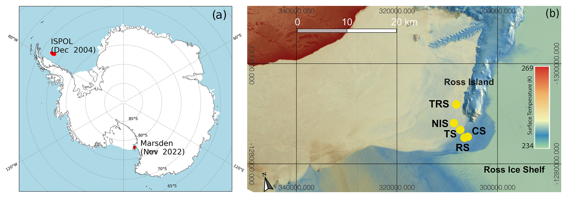
Figure 1 (a) The locations of the ISPOL and Marsden campaigns. (b) Locations of the camp site (CS), Ridge Site (RS), Transition Site (TS), New Ice Site (NIS), and Turtle Rock Site (TRS) in McMurdo Sound during the Marsden field campaign in polar stereographic coordinates. The image shows an overlay of Landsat surface temperatures over a Landsat greyscale visible image on 10 October 2022. The temperature scale is approximate only because the overlay is slightly transparent, which alters the colour.

2.2 The Marsden field campaign

A field campaign on the land-fast sea ice in the McMurdo Sound was carried out in November 2022 to assess the physical properties and spatial variability of snow on the land-fast sea ice. The campaign was part of the Aotearoa / New Zealand Marsden Fund project “Can Snow Change the Fate of Antarctic Sea Ice?” (Dadic et al., 2025; Martin et al., 2025a). Figure 1 shows the locations of the camp site (CS), Ridge Site (RS), Transition Site (TS), New Ice Site (NIS), and Turtle Rock Site (TRS) of the Marsden field campaign in McMurdo Sound, Antarctica.

The albedo observations used in this study were collected over two areas of different sea ice thickness (∼2.3 m CS and 1.2 m NIS) located at about 2 km distance from each other. Figure 1b also shows Landsat surface temperatures, illustrating potential sources of different sea ice characteristics in the region. The thickest sea ice formed earlier in the winter and was closer to the edge of the Ross Ice Shelf. Broadband albedo was measured on both locations using a pair of Kipp & Zonen CM4 pyranometers installed on a drone, while a continuous time series of broadband albedo was measured with a pair of Kipp & Zonen CMP22 pyranometers installed at about 1.2 m above the surface in a fixed station at the CS over the thicker ice. The drone's pyranometers are embedded into gimbals that ensure their horizontal alignment. However, continuous adjustment of the alignment generates vibrations that, when summed to the instrumental error, cause a total uncertainty in the measured albedo of the order of ±3 %. The uncertainty of albedo measured with the fixed CMP22 pyranometers is around ±1 %. Snow depth was measured in snow pits and along horizontal transects using a magnetostrictive device (magnaprobe), while ice thickness was measured in ice holes and along transects with an electromagnetic induction device (EM-31) carried on a sledge. The campaign was characterised by a steady temperature increase from −25 to −3 °C with a snowstorm in the last week of the campaign (27 and 28 November).

2.3 Satellite products

Data from two multispectral satellites, Landsat 9 and Sentinel 2, are used to estimate the high-resolution broadband surface albedo over the Marsden field campaign site. The instruments on board Landsat 9 and Sentinel 2 provide images at different spatial resolutions, depending on the wavelength of the spectral band, but the broadband albedo products can be calculated at 30 and 20 m resolutions respectively. The images were acquired in different channels in visible–shortwave infrared wavelengths (452–2294 and 458–2280 nm respectively) during the period of the Marsden expedition. To obtain the broadband albedo values, the Liang (2001) algorithm of narrowband to broadband albedo conversion was applied, which uses the blue, red, near-infrared, and shortwave infrared bands to estimate the broadband albedo. For the Sentinel 2 image, the L2A reflectance product with already calibrated bands is used. However, the Landsat 9 L1 image went through further processing, using the methodology proposed by Traversa et al. (2021) for high latitudes. This involved several correction steps (radiometric calibration and zenith angle, atmospheric and topographic corrections) to estimate the surface albedo. Correction for the anisotropy was not applied, since existing correction models are not able to suitably account for albedo variations at high solar zenith angles (Traversa and Fugazza, 2021). The uncertainty of the Landsat 9 albedo product, based on the applied methodology described in Sect. 2.3, is ±0.02 in polar regions (Traversa et al., 2021). For Sentinel 2 albedo imagery, an uncertainty of ± 0.05 was estimated by Naegeli et al. (2017) and Di Mauro et al. (2024).

Furthermore, the CLARA-A3 blue-sky albedo product (dates mentioned in the text refer to the central date of the monthly averaging period Karlsson et al., 2023), which has a coarser resolution of 25 km, is used to evaluate the albedo variability over the whole Weddell and Ross seas. Riihelä et al. (2024) have evaluated the mean bias of the data against a selection of high-quality in situ surface albedo measurements to be generally 10 %–15 %.

Two high-resolution satellite images from the Marsden campaign site and two lower-resolution, broader-scale satellite images – one from the ISPOL site and one from the Marsden campaign site – are utilised. The commonly used albedo products from the Moderate Resolution Imaging Spectroradiometer (MODIS, e.g. Hall and Riggs, 2021) do not cover the open ocean; thus we are not able to use them.

3 Regional oceanic and atmospheric models

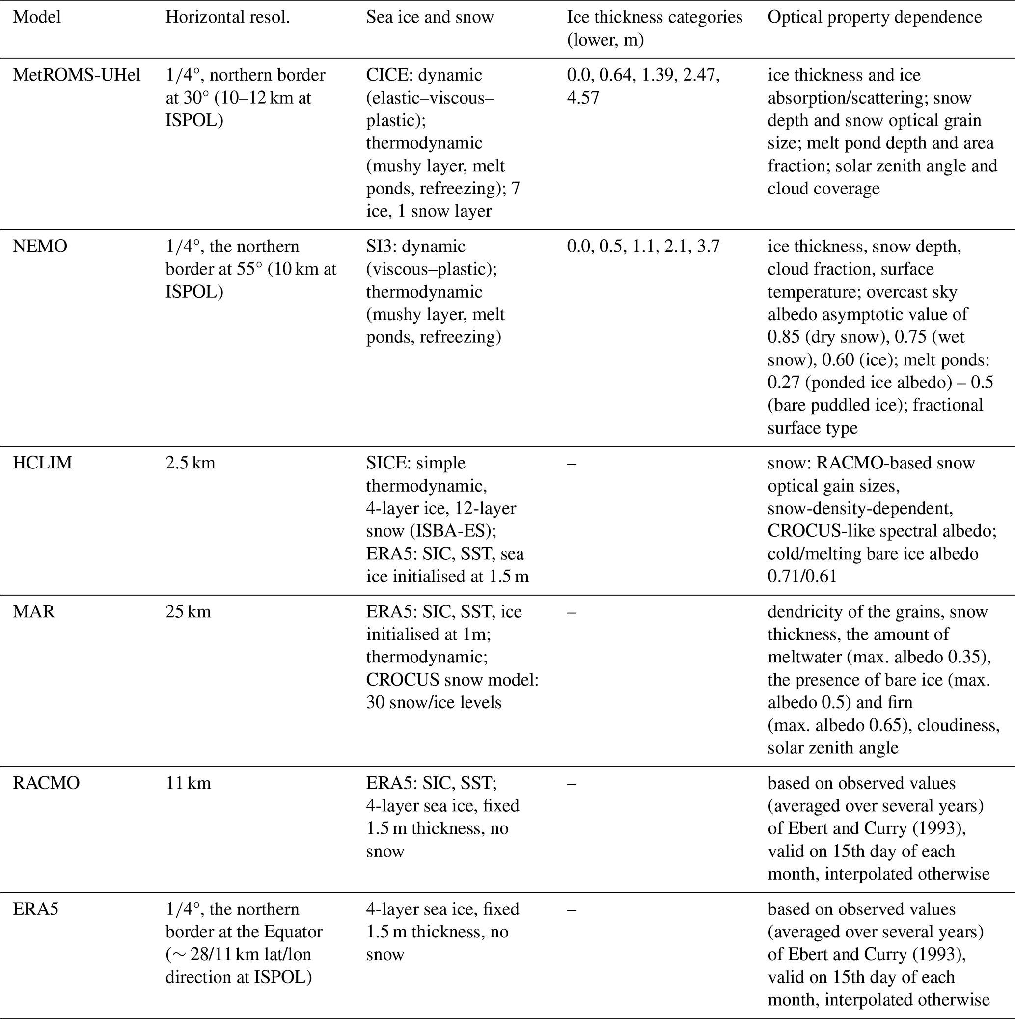
The observations are used to assess the albedo modelled by MetROMS-UHel and NEMO ocean models; the regional atmospheric models HCLIM, MAR, and RACMO; and the ERA5 reanalysis product. The sea ice and snow-related characteristics of these models are summarised in Table 1.

Ebert and Curry (1993)Ebert and Curry (1993)

Table 1 Summary of relevant model characteristics for the models used in this study. Regional oceanic models: MetROMS-UHel and NEMO. Regional atmospheric climate models: HCLIM, MAR, and RACMO. Reanalysis product: ERA5.

3.1 MetROMS-UHel

MetROMS-UHel (Naughten et al., 2018; Äijälä et al., 2025) is a coupled ocean–sea ice model. It consists of the terrain-following regional ocean model ROMS (Regional Ocean Modelling System, Shchepetkin and McWilliams, 2005) and the dynamic–thermodynamic sea ice model CICE (Hunke et al., 2022). The model uses the development version 3.7 of ROMS code and version 6.3.1 of CICE for sea ice. The model is run on a $\mathrm{1}/\mathrm{4}$° grid with the northern border at 30° S and a relocated south pole. This gives a Cartesian resolution of 8–12 km on the continental shelves around Antarctica. ERA5 reanalysis is used for atmospheric forcing. A detailed description of the model setup can be found in Äijälä et al. (2025).

The sea ice has five thickness categories and seven vertical ice layers, each having one snow layer. The lower bounds for the ice thickness categories are 0.0, 0.64, 1.39, 2.47, and 4.57 m. The model uses elastic–viscous–plastic formulation for dynamics (Hunke and Dukowicz, 2003; Bouillon et al., 2013) with an incremental remapping scheme (Lipscomb and Hunke, 2004) for advection. For thermodynamics, a mushy layer formulation is used (Turner et al., 2013), with a level-pond parameterisation (Hunke et al., 2013) with refreezing based on Stefan's law. Albedo is calculated with a Delta-Eddington multiple scattering radiative transfer model (Briegleb et al., 2007). The shortwave radiation forcing given to the Delta-Eddington model is calculated using total cloud cover, humidity, and solar zenith angle.

In the model, apparent optical properties (AOPs, e.g. albedo and transmittance) of ice and snow are calculated by the Delta-Eddington model using ice and snow microscopic inherent optical properties (IOPs, i.e. extinction coefficient, asymmetry parameter, single scattering albedo) that depend on snow depth, ice thickness, snow optical grain size, and ice absorption–scattering coefficients (Holland et al., 2012). It calculates the AOPs for three different surface types: snow-covered ice, bare ice, and ponded ice for all thickness categories. The horizontal fraction of surface type is used to get the weighted average albedo of the grid cell. The IOPs for bare and ponded ice are taken from semi-empirical modelling based on SHEBA observations over the Arctic (Light et al., 2008), and the IOPs for snow use the equivalent ice sphere approximation for specific snow grain size from Grenfell and Warren (1999).

3.2 NEMO

The ocean model NEMO (Nucleus for European Modelling of the Ocean, Madec and the NEMO System Team, 2024) is coupled with the dynamic–thermodynamic sea ice model SI3 (Sea Ice Modelling Integrated Initiative, Vancoppenolle et al., 2023). The model runs at $\mathrm{1}/\mathrm{4}$° resolution, with a northern border at 55° S, resulting in 10 km Cartesian resolution at the ISPOL location. Oceanic forcings at the border are from the reference ORCA025 simulations (Barnier et al., 2006), while the atmospheric forcings are from the JRA55 reanalysis (coherent with the forcings of ORCA025). The grid has 121 unevenly spaced vertical layers with a resolution of 1 m at the surface and up to 200 at 5000 m depth.

NEMO's SI3 has five categories of varying thickness to represent the ice pack, with upper bounds for the categories at 0.5, 1.1, 2.1, and 3.7 m. We note that the sea ice categories differ from those of MetROMS-UHel, as model setups were done separately, and respective sea ice model default categories were used. The last category has no upper bound and can represent arbitrary thick ice. The sea ice of any thickness category is described by two ice layers and one snow layer. The maximum sea ice concentration per pixel is 95 %, to account for unresolved polynyas and leads. The albedo of the snow/sea ice is calculated through empirical methods, taking into account factors such as ice thickness, snow depth, and surface temperature. The albedo parameterisations are based on Shine and Henderson-Sellers (1985) but revised following Brandt et al. (2005b) and Grenfell and Perovich (2004). The impact of melt ponds on the albedo has also been included (Lecomte et al., 2015). Melt pond properties as given by the physical level-ice scheme are characterised by the volume and level area of meltwater per unit grid cell area. They can refreeze, in which case a lid can appear, masking the effect of ponds on surface albedo.

SI3 assumes that snow, bare ice and ponded ice can coexist. However, if snow is present over sea ice, the total albedo of the grid cell is equivalent to only the snow albedo, with a deep snow asymptotic value of 0.85 for dry snow and 0.75 for melting snow (Grenfell and Perovich, 2004). If no snow is present on the ice, the total albedo is computed as a linear combination, weighted by the surface type fraction, of the bare ice albedo (which depends on ice thickness, with a maximum asymptotic value of 0.6) and the pond albedo (ranging from 0.5 to 0.27 for deep ponds), following Lecomte et al. (2011). NEMO model runs are only available for the years 1980 to 2018, hence for the ISPOL case and not for the Marsden field campaign.

3.3 HCLIM-AROME

The regional atmospheric model HARMONIE Climate cycle 43 (HCLIM, Belušić et al., 2020) using the non-hydrostatic HARMONIE-AROME physics package (Seity et al., 2011; Bengtsson et al., 2017) is set up for the two Antarctic domains with 2.5 km grid spacing. ERA5 reanalysis is used for atmospheric forcing. The HCLIM simulations use the Simple Sea-ice Scheme (SICE, Batrak, 2021). SICE is a one-dimensional thermodynamic sea ice parameterisation scheme. The external ice concentration field, in this case from ERA5, is required to define ice-covered grid cells.

SICE allows for simple bare sea ice albedo parameterisations that are dependent on surface air temperature. In this case, cold bare ice has an albedo of 0.71  and melting bare ice has an albedo of 0.61. When ice is covered by snow a different albedo scheme is used. Because snow upon the ice is an insulating layer with higher albedo and lower thermal conductivity than the underlying ice, HCLIM couples SICE, the surface modelling platform (SURFEX, Masson et al., 2013), and the Interactions Surface Biosphere Atmosphere Explicit Snow 12-layer model (ISBA-ES, Boone and Etchevers, 2001; Decharme et al., 2016) to represent snow on the ice. This is the same snow scheme used by HCLIM on land. The topmost snow layer is always less than or equal to 0.05 m thick. The scheme describes snow thermal conductivity, radiation flux, snow accumulation, melt, and snowpack compaction in the 12 snow layers. However, there are no parameterisations of specific snow-over-ice processes, such as snow–ice formation or melt ponds. Snow albedo is calculated using the method of CROCUS (Brun et al., 1992; Vionnet et al., 2012), in three ([0.3–0.8], [0.8–1.5], and [1.5–2.8] µm) spectral bands, which then are combined to the total broadband albedo. The default snow albedo depends on snow density, snow optical grain size, and ageing.

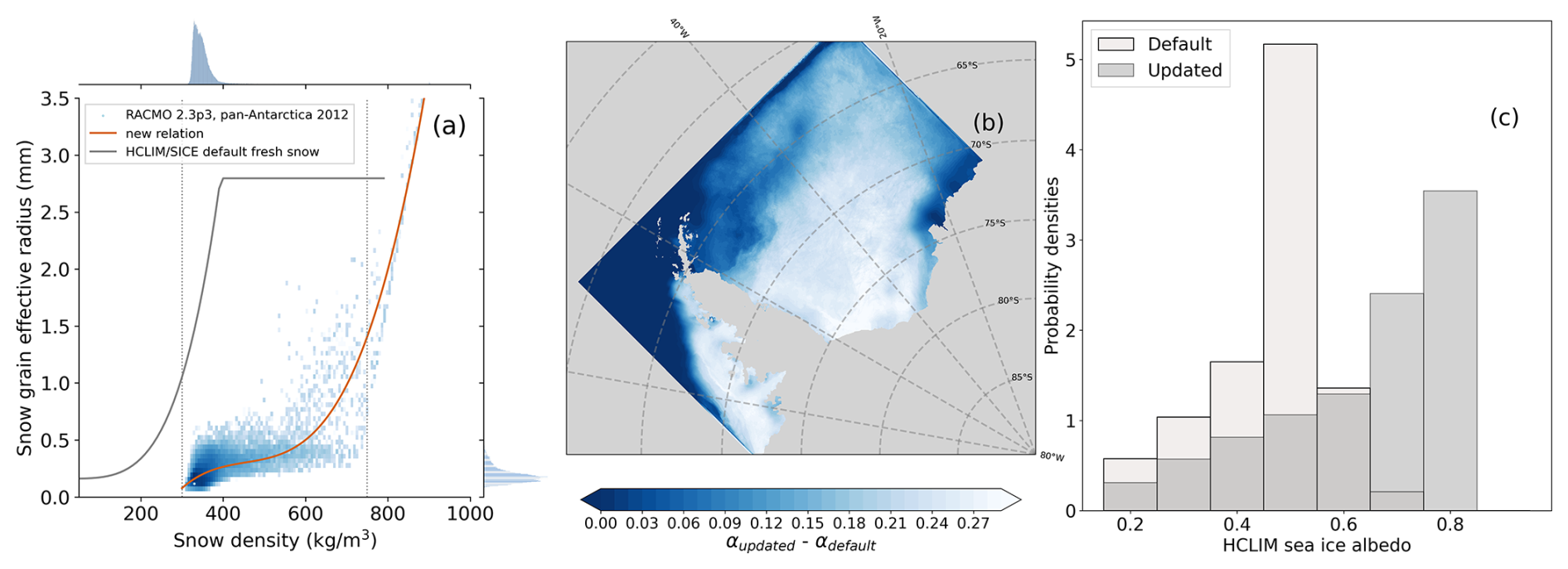
Figure 2 (a) RACMO2.3p3 2012 yearly snow grain effective radius as a function of snow density is shown as the density plot (blue shades), fitted third-order polynomial results in the updated HCLIM snow grain size to snow density relation (red solid line). The histograms show the RACMO data density. The HCLIM default relation is shown with a grey solid line. The dotted lines represent the snow density limits for sea ice in SICE and on land. (b) Differences between and (c) the probability density of both HCLIM updated and the default setting mean broadband albedo for December 2004.

The snow grain size used in the snow albedo calculation, which is only a function of snow density, determines the reflectivity of snow to shortwave radiation. In the default HCLIM setting, it is an empirical relation from Anderson (2008) measured at NOAA-ARS snow research station in Danville, Vermont, USA. It is modified further by an extra ageing term for the visual spectral band, which represents the darkening effects of snow grain metamorphism and impurities' accumulation in the snow (Vionnet et al., 2012). This term was designed for the Alps (Col de Porte) and is not representative of the polar regions. Therefore we updated the snow on sea ice and snow on land terms by setting the age-dependent term to zero.

The snow optical grain size and density relation of Anderson (2008) is not appropriate for the polar regions, where snow grain sizes are known to be smaller (Libois et al., 2015). Snow grain sizes that are too large lead to snow albedo values that are too low. This affects surface meteorology, surface energy, and mass balance. For example, the first test runs conducted for this study showed a surface temperature warm bias as large as 5 °C over sea ice compared to the ISPOL campaign measurements.

For this study, the snow grain size and density relation is updated using the output from the regional climate model RACMO version 2.3p3 (van Dalum et al., 2019, 2020, 2022). RACMO2.3p3 has updated its spectral snow albedo and radiative transfer scheme and the fresh snow grain sizes, which better correspond to Antarctic observations (Libois et al., 2015). Figure 2a shows the updated snow grain size to snow density relation together with the HCLIM default relation. In the default HCLIM setting, only large grain sizes are allowed, which leads to maximum snow albedo values of 0.75. With the improved grain sizes, the fresh snow albedo can reach a more realistic 0.85. The resulting differences in the monthly averaged broadband albedo are shown in Fig. 2b and c and are as large as 0.3.

3.4 MAR

The Modèle Atmosphérique Régional (MAR) is a hydrostatic regional atmospheric model specifically developed for the polar areas (Gallée and Schayes, 1994). For this study, a pan-Antarctic domain with a 25 km resolution (305×272 grid points) and 24 vertical levels, ranging from 2 m to 17 km above the surface, is used. ERA5 reanalysis is used as a lateral atmospheric forcing and sea surface temperature/sea ice cover. The sea ice thickness is initialised from 1 m. Snow can accumulate at the surface of the sea ice afterwards. Sea ice can also melt to a 0.1 m minimal value.

The snow–ice module includes submodules for surface albedo, meltwater refreezing, and snow metamorphism, based on the snow model CROCUS (Brun et al., 1992; Gallee et al., 2001). Thirty levels were used to represent the snowpack over Antarctica and the surrounding sea ice. Snow albedo in the CROCUS model is calculated in three separate spectral bands as a function of the snow properties in the top 3 cm of the snowpack. The snow albedo depends on the impurities in the snow (ageing term) and the optical diameter of snow grains. Unlike in HCLIM, the snow optical diameter also takes into account snow metamorphism, based on empirical laws describing the evolution rate of the type (dendric/non-dendric) and size of the snow grains (Brun et al., 1992). As described above for the HCLIM model, the CROCUS model was not initially made for polar regions, so the same correction was applied by setting the snow ageing term to 0. Hence, the snow albedo of MAR has the same three-band scheme as HCLIM, but MAR prognostically simulates the snow optical grain size, while HCLIM estimates this grain size from the snow density. If no snow is present over the sea ice, then the albedo of the bare ice varies exponentially between 0.55 and 0.5 as a function of accumulated meltwater (Lefebre et al., 2003; Tedesco et al., 2016). Finally, if the snow depth is thinner than 0.1 m, the total albedo transitions linearly between snow albedo to bare ice albedo.

When evaluating MAR albedo during the Marsden campaign, the values from the closest sea ice grid point, centred at 77.79° S, 166.71° W, are used.

3.5 RACMOp2.4

The polar version of the Regional Atmospheric Climate Model (RACMOp2.4 van Dalum et al., 2024) consists of two major parts; the dynamical core of HIRLAM (Undén et al., 2002) that models large-scale motions in the atmosphere and the physical parameterisations of the IFS (ECMWF, 2020), which represents physical processes on the sub-grid scale. This includes, for example, a cloud, turbulence and precipitation scheme. Additional parameterisations have been added in RACMO for a dedicated glaciated land surface tile, such as a multi-layer snow scheme, firn-densification modules, grain size evolution, and melt and refreezing parameterisations.

The RACMO version used in this study, version 2.4p1, has been developed recently and includes changes in several key aspects with respect to previous model versions (van Dalum et al., 2024). The IFS physics parameterisations have been updated from cycle 33r1 (ECMWF, 2009) to cycle 47r1 (ECMWF, 2020). This includes changes in all major schemes in particular in the new cloud scheme, and a new lake model is introduced. Other changes include a new multi-layer snow scheme for seasonal snow on non-glaciated surfaces and a new land-ice mask with fractional ice cover, resulting in a better representation of partly glaciated regions. A detailed description can be found in van Dalum et al. (2024). For experiments used in this study, RACMO is run on an 11 km horizontal resolution grid and is forced by ERA5 at the lateral boundaries.

As RACMO is not coupled to an ocean model, the sea ice extent is prescribed by ERA5. RACMO uses the ECMWF IFS model for sea ice, which employs a four-layer sea ice slab with a fixed maximum thickness of 1.5 m. There is no snow modelled on top of sea ice. The albedo is based on Ebert and Curry (1993) and thus does not depend on snow conditions. Instead, monthly sea ice albedo values for the Arctic Ocean, valid on the 15th of each month, are linearly interpolated to the forecast time. For the Antarctic, the seasonal cycle is shifted by 6 months. The bare sea ice albedo represents summer months, while the dry snow albedo is applied during winter months, with both direct and diffuse components. The albedo is derived using separate values for four spectral bands in the near-infrared and visible light, and the broadband albedo is the sum of the spectral albedos weighted by the relative solar flux in each wavelength region and further weighted by the direct and diffuse fractions. While this parameterisation scheme intends to capture key surface, cloud, and atmosphere effects, the albedo values are climatological means and do not depend on the state of the surface and atmosphere within the RACMO model. For example, the effect of fresh snowfall on the albedo on sea ice during summer is therefore often not captured properly, as the albedo model does not take the actual conditions into account.

3.6 ERA5

Given the findings of Pohl et al. (2020), Müller et al. (2024), and Batrak et al. (2024) that highlight the limitations of ERA5 sea ice albedo over the Arctic, ERA5 is included in this analysis over Antarctica. In ERA5, the sea ice concentration is given by the Ocean and Sea Ice Satellite Application Facility (OSI SAF) (409a) dataset (from 1979 to August 2007), and the OSI SAF open dataset (September 2007 onward). Like RACMO, ERA5 also uses the ECMWF IFS model for sea ice. ERA5 considers the Marsden CS to be on land, not on sea ice. When evaluating ERA5 albedo during the Marsden campaign, the values from the closest sea ice grid point, centred at 77.85° S, 166.54° W, are used. Since HCLIM, MAR, and RACMO use sea ice concentrations from ERA5, it can be assumed that these models extrapolate the sea ice concentrations from adjacent ERA5 ocean grid points to areas classified as land in ERA5.

4 Results

4.1 Atmospheric conditions

The model's ability to accurately reproduce top-layer snow and ice conditions is influenced by atmospheric modelling (as in HCLIM, RACMO, and MAR) or by the atmospheric forcing (as in MetROMS-UHel with ERA5 or NEMO with JRA55), particularly during the melt season. The comparison between modelled and observed 2 m temperature is presented in Fig. 3, while additional atmospheric variables such as air pressure, relative humidity, wind direction, and wind velocity are provided in Figs. A1 and A2.

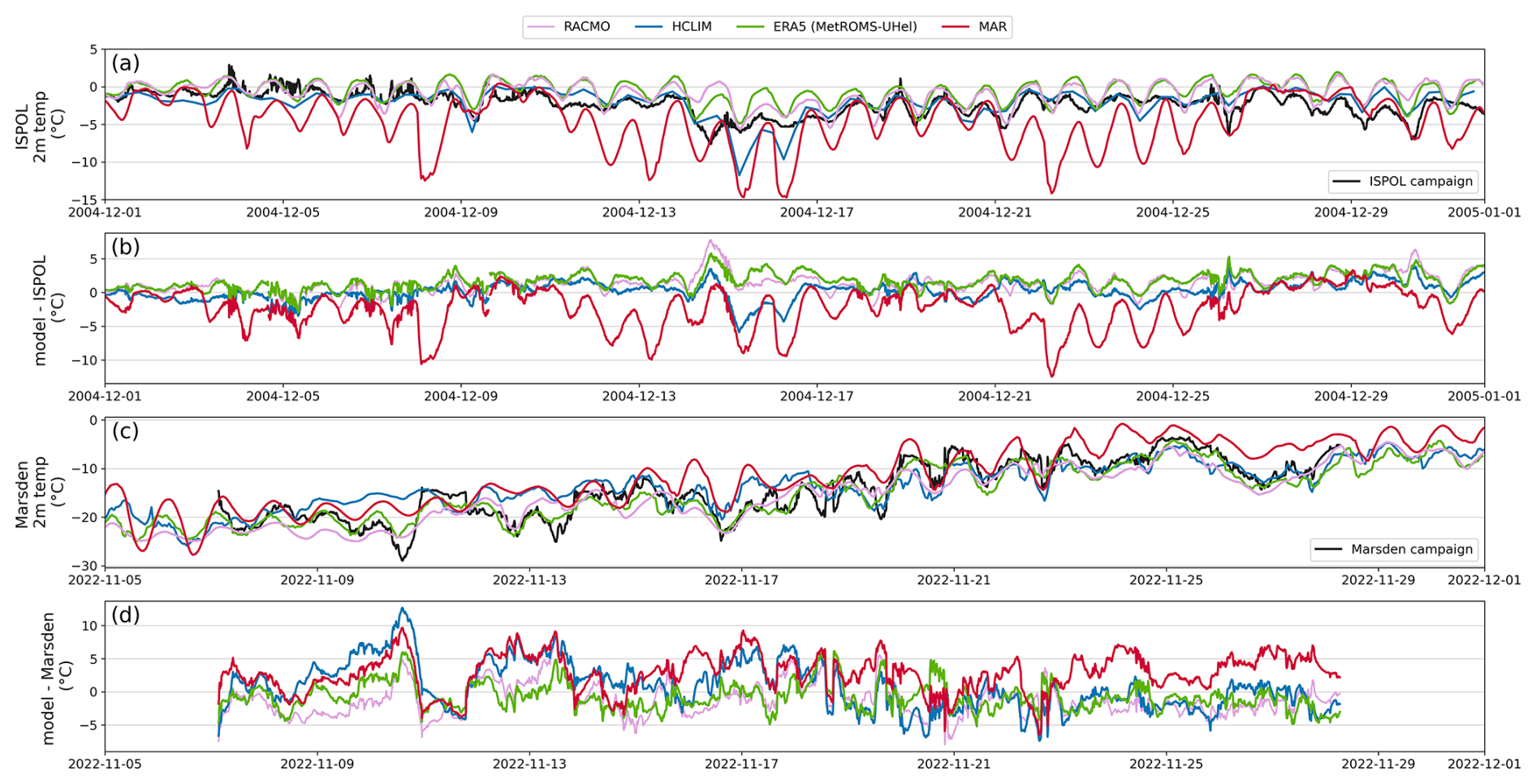
Figure 3 Modelled and observed 2 m temperature and the temperature differences during the ISPOL campaign (a–b) and Marsden campaign (c–d).

HCLIM reproduces the surface temperature observed during the ISPOL campaign best (with a mean difference of 0.2 °C), as well as the surface pressure and wind speed and direction. RACMO and ERA5 have, on average, a 1.4 and 1.6 °C warm bias, respectively, indicative of the low sea ice albedo, as discussed later. ERA5, with a resolution of 0.25° (approximately 28 km), exhibits a temperature pattern comparable to the 11 km resolution RACMO. In contrast, MAR, which has the coarsest spatial resolution of the models in the set at 25 km, displays significant diurnal variability and is, on average, 2.3 °C colder than observations, with deviations reaching up to 13 °C.

The conditions during the Marsden campaign were notably different – the air temperatures were well below freezing (mostly below −10 °C). The Marsden field campaign took place in a challenging region for models, located a few kilometres north of Ross Island (see Fig. 1). Notably, in both ERA5 and MAR, the Marsden field campaign site is inaccurately represented as land rather than sea ice. Even so, HCLIM, RACMO, and ERA5 differ by only 0.8, 1.2, and 0.8 °C from the observations. Figure 3 shows that on average, MAR exhibits a 2.8 °C warm bias and pronounced diurnal temperature fluctuations. Figure A2 reveals the problems that atmospheric models have in simulating the correct wind direction over the Marsden campaign site: instead of the observed predominantly southerly winds, the models predicted more easterly winds. The reason for this discrepancy is the resolution differences and the proximity of Ross Island and the Ross Ice Shelf.

We have included total cloud coverage of the models in Fig. A3. There are considerable differences in cloud cover over the ISPOL and Marsden campaign sites between the models, which can only partly be explained by differences in resolution. The snow and ice albedo can be, on average, 4 %–6 % higher under cloudy conditions compared to clear skies (Key et al., 2001). However, only MetROMS-UHel, MAR, and NEMO account for the effect of clouds in their sea ice albedo parameterisations, whereas HCLIM, RACMO, and ERA5 do not include this effect.

4.2 Comparison between modelled and measured sea ice albedo

In situ measurements provide a detailed understanding of the temporal variability of sea ice albedo, along with general snow and ice characteristics. However, these measurements fall within the sub-grid scale of the models used in this study, with HCLIM offering the highest resolution at 2.5 km. Additionally, both campaign locations present challenges for model reproduction – McMurdo Sound is characterised by complex topography, and the ISPOL campaign took place close to the edge of the modelled December sea ice extent. Figure 4 shows the month-long ice and/or snow albedo time series. Table 2 presents the mean albedo values with standard deviation. Since both campaigns measured on either an ice floe or land-fast ice, we compare these measurements to the modelled sea ice albedo rather than the modelled total albedo, which would include open-water albedo if present in a model grid cell.

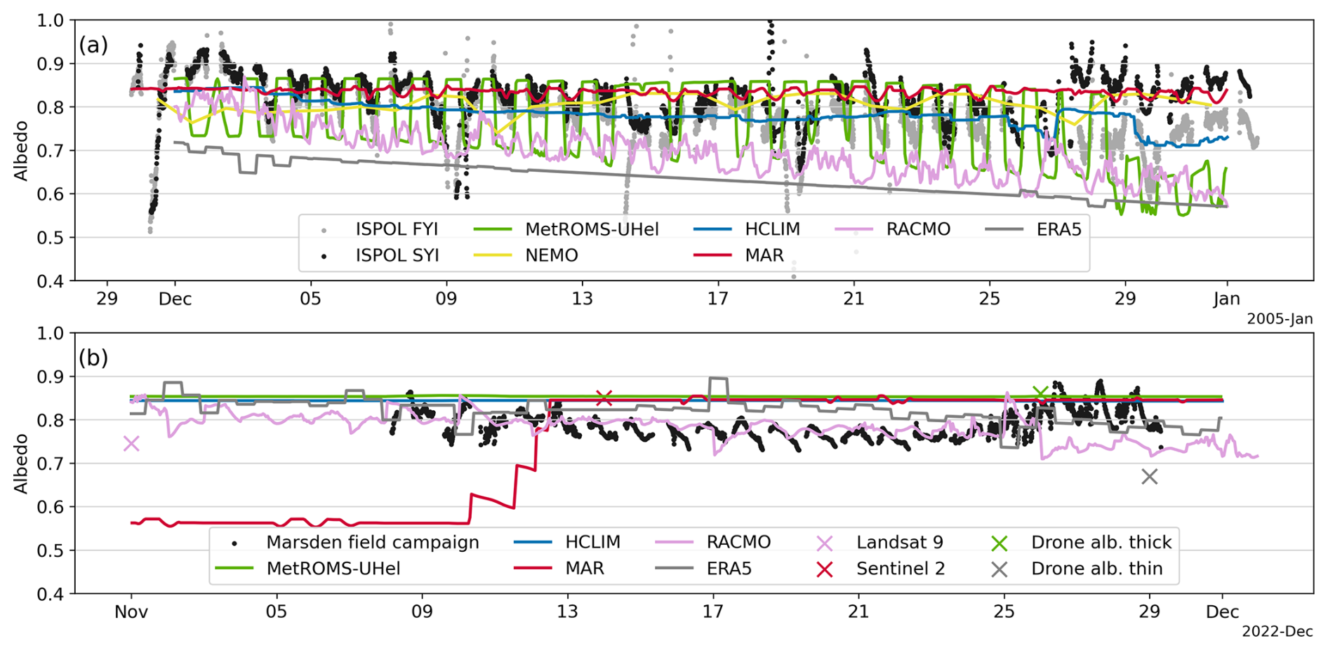
Figure 4 Observed and modelled sea ice albedo time series for the ISPOL (a) and the Marsden (b) campaigns. Some models, such as MetROMS-UHel and HCLIM, output separate albedo values for snow and ice. Others, like MAR, NEMO, and RACMO2.4, provide a grid-box-averaged albedo that combines contributions from ocean, ice, and snow. For these models, we derived the snow and ice albedo by isolating the ocean contribution using sea-ice-concentration data. Sea ice albedo derived from high-resolution Landsat 9 and Sentinel 2 images is shown here and analysed further in Sect. 4.5. The mean sea ice albedo values from drone measurements are shown here but analysed in Sect. 6.

Table 2 Average observed and modelled snow/ice albedo values and corresponding temporal standard deviations due to variability (in brackets) over the campaign period. ISPOL campaign site: measurements done at the FYI and SYI radiation sites. Marsden campaign: measurements conducted at the fixed radiation station at the camp site (CS). NEMO model runs are only available for the ISPOL case and not for the Marsden field campaign.

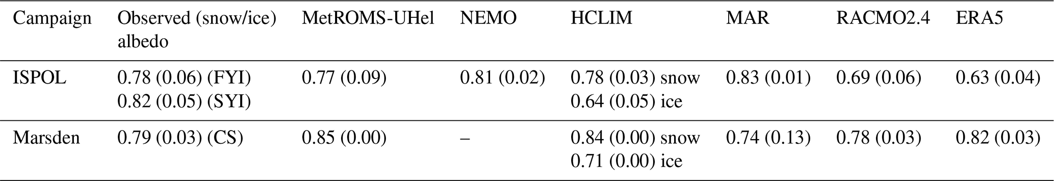
On the ice floe, to which RV Polarstern was moored during the ISPOL campaign, snow depth decreased on average from 32 to 14 cm on FYI and from 95 to 83 on SYI during December 2004 (Nicolaus et al., 2009a). On the FYI, the thinner snowpack had a mean albedo of 0.78 (SD = 0.06), while on SYI the thicker snow cover had a mean albedo of 0.82 (SD = 0.05). The standard deviation of albedo primarily reflects the diurnal variability observed during the ISPOL campaign, driven by near-melt snow conditions during the day, refreezing at night, and changes in the solar zenith angle. Additional changes in observed albedo were influenced by snowfall, drifting snow, and the relocation of the equipment (Vihma et al., 2009).

The snow on top of the 1 to 4 m thick land-fast ice in the McMurdo Sound had a relatively thin (∼0.21 m, CS) or patches of thin (∼0.02 m, NIS) snow on top. Snow thickness variability in the observed range between 0 and 0.2–0.3 m has a big impact on the albedo. For densely packed, fine-grained snow, the snow layer becomes semi-infinite – meaning that further increases in depth no longer affect snow reflectance – at a depth of approximately 0.10 m (Zhou et al., 2003).

Overall, a mean surface albedo of 0.79 (SD = 0.03) was observed. A snowstorm during the last week of the campaign led to an increase in albedo which reached up to 0.9. The observed albedo was primarily influenced by variations in drifting snow accumulation patterns within the field of view of the downward-looking pyranometer. The snow was often reported as optically translucent, allowing the bare ice beneath to be visible. In nature, bare ice albedo varies between 0.1 and 0.7 depending on the ice thickness and the presence of cracks, melt, brine pockets, and air bubbles (Allison et al., 1993; Brandt et al., 2005a). Bare ice albedo values above 0.56, however, have been observed only during melting, when the surface of the ice decomposes into white ice or “surface scattering layer”. White ice is typical of summer Arctic sea ice but has never been observed over Antarctic sea ice (Grenfell and Maykut, 1977). However, Traversa and Di Mauro (2024) recently reported the presence of this “surface scattering layer”, which they referred to as the weathering crust, over blue ice areas of ice shelves of the Northern Victoria Land, Antarctica.

Considering that the measurements are from a single point location, while model output represents grid cell averages, the models reproduce high albedo values and diurnal variability at the ISPOL location but struggle to accurately capture the albedo variability at the Marsden site. MetROMS-UHel successfully captures both the overall level of albedo and the strong diurnal variability observed during the ISPOL case, with a mean modelled albedo of 0.77 (SD = 0.09). In the Marsden case, MetROMS-UHel suggests a constant albedo of 0.85. NEMO output was only available for the ISPOL case study, in which case it has a monthly mean albedo of the sea ice of 0.81 (SD = 0.02). As only daily NEMO albedo fields were saved, any modelled diurnal variability is lost for this analysis.

HCLIM simulates a snow albedo of 0.78 (SD = 0.03) for the ISPOL case, close to the observed albedo over SYI. The HCLIM snow albedo in the Marsden campaign case is 0.84 (SD = 0.00). The HCLIM bare ice albedo for the Marsden case is 0.71 (SD = 0.00), coming from the simplistic two-value (0.61 or 0.71) parameterisations of bare ice albedo in the model. HCLIM bare ice albedo is too high, as bare ice albedo values above 0.56 are unlikely in this context.

MAR simulates a monthly mean albedo of 0.83 (SD = 0.01) and 0.74 (SD =  0.13) for the ISPOL and Marsden field campaigns respectively. A small diurnal variation is present in the model output at the ISPOL location but not to the extent of the observations or of the MetROMS-UHel simulations. A significant increase in MAR's surface albedo, from 0.55 to 0.85, occurred between 10 and 13 November when a thin layer of snow fell within the previously bare ice grid cell in the model, resulting in an immediate rise in the modelled albedo.

RACMO and ERA5 both use time-interpolated monthly albedo values based on the albedo scheme developed by Ebert and Curry (1993) for the Arctic sea ice. Differences between the two models come from the resolution: RACMO was run at 11 km resolution, but ERA5 has a 0.25° (∼28 km) resolution. At the ISPOL location, both RACMO and ERA5 had lower surface albedo values than expected from observations, with RACMO at 0.69 (SD = 0.06) and ERA5 at 0.63 (SD = 0.04). However, over the Marsden campaign site, RACMO more accurately represents the observed conditions compared to all other models. In this instance, the assigned monthly average sea ice albedo values of Ebert and Curry (1993) align with the albedos observed in this case study. ERA5 differs in this case, as the values from the nearest sea ice grid point are used because the campaign site is inaccurately represented as land rather than sea ice.

Comparisons with the Marsden CS measurements come with a caveat: to analyse the sea ice properties, instead of land, the EAR5 and MAR model values from the closest sea ice grid point were used. In both cases, the nearest sea ice model grid point is not located at the CS site but towards NIS or TRS sites or farther. The proximity of Ross Island and the Ross Ice Shelf results in rapidly changing sea ice properties over short distances, as described in Sect. 4.3 and 4.4. While observations taken farther from land – such as during the ISPOL campaign – offer a cleaner comparison, we work with the data available.

Overall, when compared to measurements from the ISPOL and Marsden campaign sites, the models reproduced the conditions observed during the ISPOL campaign but did not accurately simulate the conditions during the Marsden campaign. For the ISPOL case, all modelled albedos, except RACMO and ERA5, fell within the observed ranges. The MetROMS-UHel model accurately captured both the magnitude and diurnal variability of snow albedo for the ISPOL case. In contrast, RACMO's prescribed albedo was consistently about 0.1 too low throughout the ISPOL campaign season. The snow and ice conditions in the Marsden campaign area were very different. All models, except RACMO, simulated sea ice albedo as being dominated by cold, snowy conditions and were unable to account for the patchiness and drifting snow patterns observed in the region. RACMO accurately predicted the observations from the Marsden campaign, despite relying on Ebert and Curry (1993) monthly averages of sea ice albedo for its predictions.

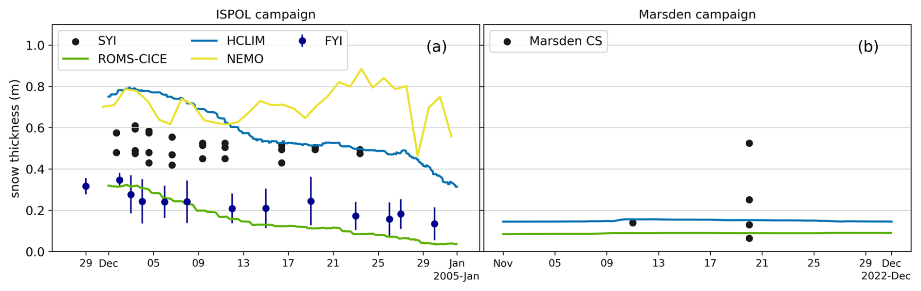
Figure 5 Snow thickness over sea ice time series for the ISPOL (a) and the Marsden campaigns (b). ISPOL campaign: measurements which were taken closest to the FYI and SYI radiation sites. Marsden campaign: measurements conducted near the fixed radiation station at the camp site (CS). For the models, the grid-box-averaged snow thickness is shown if available. All the other models provide hourly output, whereas NEMO provides daily output. ERA5 and RACMO do not have snow on sea ice. MAR provides combined snow and ice thickness and is excluded here.

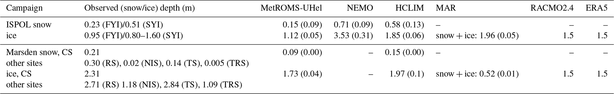
Table 3 Measured in situ and grid-box-averaged modelled snow and ice thicknesses and corresponding temporal standard deviations due to variability (in brackets) over the campaign period. ISPOL campaign: measurements over FYI and SYI. Marsden campaign: measurements from camp site but also from Ridge Site (RS), Transition Site (TS), New Ice Site (NIS), and Turtle Rock Site (TRS), shown in Fig. 1.

4.3 Comparison between modelled and measured sea ice and snow thickness

A certain optical thickness of snow is required to obscure the underlying ice, and similarly, bare ice must reach a specific thickness to mask the darker ocean beneath. Therefore, to interpret the comparison between modelled and observed albedo, it is valuable to analyse the modelled snow and ice thickness in comparison to the observed values. During both campaigns, ice and snow thicknesses were measured at multiple locations across the campaign sites, leading to broad distributions, especially of snow thicknesses across both sea ice campaign regions. Only NEMO and MetROMS-UHel have sub-grid ice categories, which are used to analyse such unresolved spatial variability of sea ice thickness in Sect. 4.4. Here, modelled grid-box-averaged sea ice thickness and snow thickness are examined and compared with measurements taken closest to the location of the albedo measurements. The models are not regridded to a common low-resolution grid in order to preserve high-resolution information.

Figure 5 and Table 3 compare the measured snow thickness in the ISPOL and Marsden campaigns with grid-averaged model outputs. Generally, the thicker the sea ice, the greater the ice freeboard and the amount of snow it can support.

The ISPOL location measurements were done over the FYI and SYI. MetROMS-UHel snow thickness follows the level and trend of the ISPOL FYI measurement site: 0.35 m thickness at the beginning of the month and only a few cm thick at the end. The grid-box-averaged bare sea ice thickness underneath is 1.15 m. HCLIM predicts thicker snow, 0.8 m at the beginning of the month, dropping to 0.4 m at the end of the month, with a 1.85 m sea ice underneath the snow. NEMO also predicts a thicker, 0.71 m, snow cover over a 3.5 m bare sea ice. While HCLIM shows a decrease in snow thickness over the month, NEMO snow thickness is variable but not decreasing. The snow cover modelled by NEMO and HCLIM is thicker than measured at the ISPOL SYI and FYI locations. However, there were sites at the ISPOL ice floe where snow thicknesses were in that range (Nicolaus et al., 2009a). MAR only provides the combined sea ice and snow depth output, which amounted to 1.96 m. RACMO has a fixed sea ice thickness of 1.5 m and no explicitly modelled snow on top (Table 1).

During the Marsden campaign, snow thickness measurements were done in multiple locations (averages given in Table 3). Reportedly, the thicker ice at CS was covered by a thin (0.21 m) but heterogeneous snow layer with small spots (1–2 m²) of bare ice. The thinner ice (at NIS and TRS) was mostly bare with small patches (1–2 m²) of thin (approximately 1–2 cm) snow (Martin et al., 2025a). In Fig. 5, the model output is exclusively compared to the measurements at CS, closest to the radiation time-series measurements. The models predict a thin (0.09 m (MetROMS-UHel) or 0.15 m (HCLIM)), uniform snow cover. The thickness of bare sea ice is modelled to be 1.73 and 1.97 m for MetROMS-UHel and HCLIM respectively. Because MAR considers the Marsden CS to be on land, and the closest sea ice grid point is further away, MAR's snow and sea ice thickness are not fully representative. MAR's combined sea ice and snow depth is 0.50 m at the start of the period and increases to 0.53 m throughout 10–12 November, causing the increase of albedo seen in Fig. 4 due to snowfall. ERA5 and RACMO sea ice have a constant and uniform thickness of 1.5 m and no modelled snow.

4.4 Sub-grid sea ice characteristics around the Marsden campaign site

Even within a small sea ice region, multiple types of sea ice can be present. NEMO and MetROMS-UHel have sub-grid ice categories, which can be used to analyse the unresolved spatial variability of sea ice thickness within each model grid cell. However, NEMO output for the Ross Sea in November 2022 was unavailable, as the model data only extend up to 2018. Therefore, we compared MetROMS-UHel with the Marsden campaign measurements from November 2022, and with NEMO for November 2004. The model's intrinsic bare ice characteristics per category remain consistent year to year, while the presence of ice types, the fractional snow cover, and the cloud coverage change.

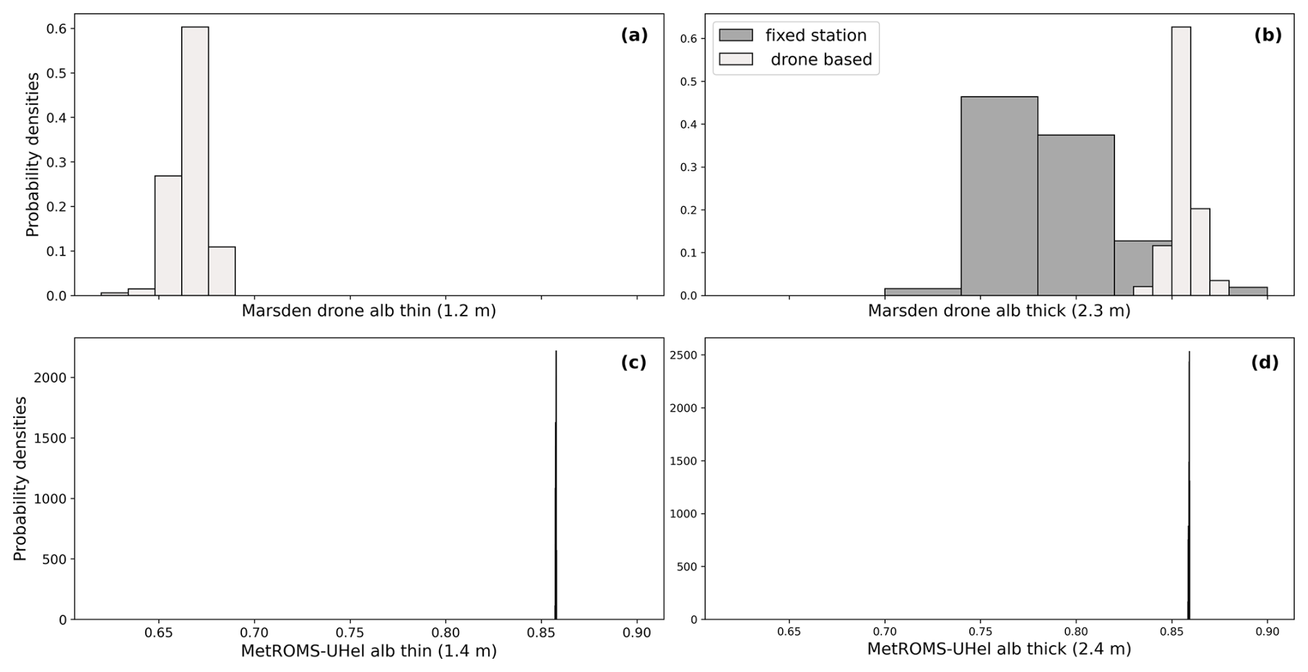
Figure 6 Probability distributions of drone-based or fixed-station sea ice albedos at the Marsden field campaign (a, b) for November 2022, measured over thinner ice (1.2 m; a) and thicker ice (2.3 m; b), and the modelled MetROMS-UHel albedos (c, d) for closest thickness categories (1.4 and 2.4 m respectively).

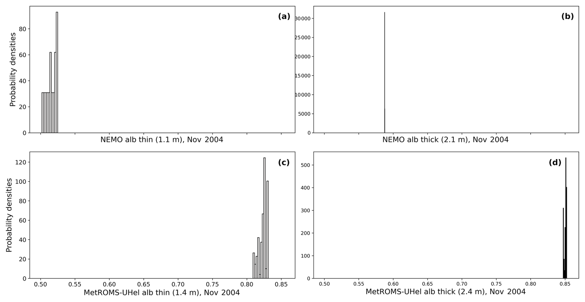
Figure 7 Probability distributions of the modelled NEMO sea ice albedos (a, b) for 1.1 and 2.1 m ice categories and the modelled MetROMS-UHel albedos (c, d) for closest thickness categories (1.4 and 2.4 m respectively) for November 2004 Marsden field campaign location.

Figure 6a–b show the probability distributions of the albedo measured from a drone flying a single vertical profile at an altitude between 30 and 50 m over thick ice and another profile between 30 to 70 m altitude over thin ice with patchy snow cover. The flight lasted ∼10 min, without significant changes in solar zenith angle and cloud conditions. At these heights, the footprint of the drone's downward-facing pyranometer, calculated as the area contributing to 90 % of the received radiation, has a radius ranging from 90 m (at 30 m height) to 210 m (at 70 m height). Hence, these probability distributions represent the albedo averaged over footprints of ∼0.02–0.04 km² and, therefore, are better suited for validating satellite albedo products and model simulations than the fixed-station measurements.

Over the thick ice, the downward-facing pyranometer of the fixed station mostly receives the radiation reflected from the surface type located just underneath it (∼ a few m²), having a mean albedo of 0.80. In contrast, the pyranometer on the drone captures radiation from all surface types within its footprint, weighted by their respective fractions. This resulted in a higher mean albedo of 0.86. Since the fraction of bare ice was significantly smaller than that of snow-covered ice, the drone measured more radiation reflected from the patchy snow cover compared to the bare ice.

Starting from the altitude of 30 m and above, the measured albedo did not change with altitude, meaning that the spatial distribution of surface albedo variability included in the footprint of the downward facing pyranometer did not change with increasing footprint radius. Hence, the small variations in the drone-based albedo observed from 30 m above the surface and at higher altitudes were associated with measurement errors (caused for instance by small vibrations of the drone and small deviations from the horizontal alignment of the pyranometers when compensating for changes in wind speed) rather than with spatial variability. The spread of the drone-based albedo probability distributions, which represent the measurement uncertainty during ∼ 10 min flight, is much narrower than the spread of the probability distribution of the albedo measured from the fixed station close to the surface during a 1-month-long observation period (Fig. 6b).

The temporal variability of the fixed-station albedo is caused by the change in solar zenith angle; the changes in cloud cover; the occurrence of precipitation and snowdrift; and, to a lesser extent, snow metamorphism (which was weak because the surface temperature was well below freezing for the whole period). During the studied period, the daily minimum solar zenith angle decreased from 60.5 to 56.2°, and cloud cover ranged from 0 to 8 oktas. The continuous snow drift, snow erosion, and formation of snow patches and dunes changed the snow thickness in the footprint area of the fixed downward-looking pyranometer in a similar way to that in the surrounding area. Hence, we can argue that the probability distribution of the fixed-station albedo illustrates the effects of both temporal and spatial albedo variability, assuming that the snow thickness variability that occurred right below the pyranometer is a good proxy for the larger-scale spatial variability.

Drone-based albedo measurements over the thin ice showed a mean albedo of 0.66, as the ice surface was dominated by bare ice with snow patches. The thinner and younger ice was formed in August 2022, which is why it had less snow than the thicker ice, which was formed in March 2022.

The modelled MetROMS-UHel albedos for the 1.4 and 2.4 m ice thickness categories are included in Fig. 6c–d. The selected model thickness categories are the closest to the observed sea ice thicknesses. The modelled NEMO albedos for 1.1 m and 2.1 m ice categories are compared to the modelled MetROMS-UHel albedos for the 1.4 and 2.4 m ice thickness categories for November 2004 of the Marsden field campaign site location in Fig. 7a–b.

The discrepancy between the observations and the models over the thinner ice is large: Δ_mean=0.2 for MetROMS-UHel. In this case, the MetROMS-UHel modelled albedo is snow-dominated, as both ice categories are covered with a layer of snow. The same situation occurs in 2004, where the MetROMS-UHel albedo is also dominated by snow, but NEMO had snow-free conditions. NEMO's bare ice albedo depends mainly on ice thickness, with a maximum albedo value of 0.5 for 1 m thick sea ice and approaching an albedo value of 0.6 for 1.5 m and thicker ice, with additional adjustments based on cloud fraction.

The drone-based albedo measurements over the thicker ice are reproduced by MetROMS-UHel, with differences between the average values of the two distributions being negligible (Δ=0.004). MetROMS-UHel albedo has a narrower distribution (SD = 0.00) than the observed distribution (0.02). NEMO's albedo is 0.59, which is close to the maximum value assigned by the model to bare ice albedo but is far too low compared to the observations.

These model-to-observation comparisons demonstrate that direct comparisons with surface-based point measurements are not meaningful when there is metre-scale spatial heterogeneity in surface albedo. MetROMS-UHel and NEMO have information on sub-grid ice categories, but the snow on the ice, if any, covers it uniformly. The comparisons also show that the correct estimate of the snow cover depth is essential to correctly model the sea ice albedo.

4.5 Spatial albedo variability over the McMurdo Sound area

Expanding the analysis to cover larger areas that align with the model resolution is a fairer evaluation of the models. This section compares the model output to high-resolution (30 m Landsat 9 and 20 m Sentinel 2) satellite images over a limited area (260×260 km² Landsat 9 and 110×110 km² Sentinel 2) in McMurdo Sound, which includes the Marsden campaign site. In Sect. 4.6, the comparison is expanded to lower-resolution satellite observations over larger areas, covering the entire Ross and Weddell seas.

Landsat 9 albedo observations on 1 November in Fig. 8, and Sentinel 2 observations on 14 November 2022 in Fig. 9, are compared to the modelled total albedo of sea ice (combination of ice, snow and ocean). The satellite images show a variety of albedo values over the region: open ocean with an albedo of around 0.1, thicker bare land-fast ice with an albedo of 0.7 and higher depending on the snow cover, and everything in between. The image also shows bare and snow-covered land.

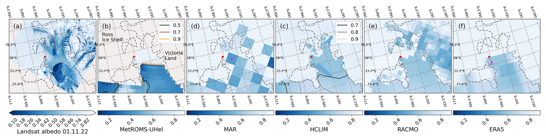
Figure 8 Landsat 9 albedo over the Marsden campaign site (a), on 1 November 2022 compared with the modelled albedo, closest hourly output to the satellite flyover, of MetROMS-UHel (b), MAR (c), HCLIM (d), and RACMO (e), and ERA5 reanalysis (f). For these maps and the ones below, where relevant, we use combined bare ice or snow and ocean albedo (with a value of 0.06) using sea ice concentration for scaling; for MetROMS-UHel, we use the total snow and ice albedo and combine with ocean albedo similarly; for MAR, we used albedo averaged across all surface types. Snow fraction contours (0.5, 0.7, and 0.9 with black, brown, and yellow lines) are shown atop MetROMS-UHel. Sea ice concentration contours (0.7, 0.8, and 0.9 with black, grey, and light-grey lines) are shown atop HCLIM, which seem to describe the spatial variability of the albedo better. Red points indicate the location of the Marsden field campaign site, and the magenta points are the locations where the model values were taken.

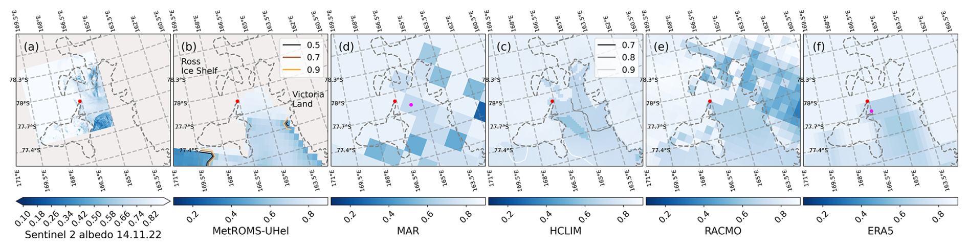
Figure 9 Sentinel 2 albedo over the Marsden campaign site, on 14 November 2022 and the modelled total albedos, closest hourly output to the satellite flyover, of MetROMS-UHel (b), MAR (c), HCLIM (d), RACMO (e), and ERA5 reanalysis (f). Snow fraction contours (0.5, 0.7, and 0.9 with black, brown, and yellow lines) are shown atop MetROMS-UHel, but sea-ice-concentration contours (0.7, 0.8, and 0.9 with white, grey, and black lines) are shown atop HCLIM, which seem to describe the spatial variability of the albedo better.

Overall, the albedo in the region increased between the two dates. This is also evident at the Marsden campaign site, shown in Fig. 4, where the Landsat 9 sea ice albedo is lower than the in situ observations, while the Sentinel-2 albedo is higher. Except over the land-fast sea ice, where concentrations remain unchanged, sea ice concentrations in McMurdo Sound increased locally, which explains the observed albedo increase over the sea ice. The higher albedo on the latter date could have various causes, such as solar zenith angle (SZA) differences due to satellite fly-by times, using different satellite sensors and data processing variations. The uncertainty of the Landsat 9 albedo product is ± 0.02 in polar regions, while that of the Sentinel-2 albedo imagery is ± 0.05. We can estimate the effect of solar zenith angle on snow and ice albedo between the two dates using parameterisation from Gardner and Sharp (2010). Assuming pure, dry fresh snow with an albedo of 0.9 and a solar zenith angle of 0°, the albedo reduction due to the solar zenith angle at the Landsat 9 overpass (SZA=70.8°) is 0.038. For the Sentinel 2 overpass (SZA=67.3°), the corresponding albedo effect is 0.036. For ice and snow with lower albedo values, the effect is more pronounced – for example, sea ice with an albedo of 0.5 experiences albedo effects of 0.1, for both SZA=70.8 and 67.3°. However, the difference in albedo between the two observation dates remains small, on the order of 0.01 or less.

Figure 10 Sea ice albedo distribution (land removed) over the Landsat 9 image domain.

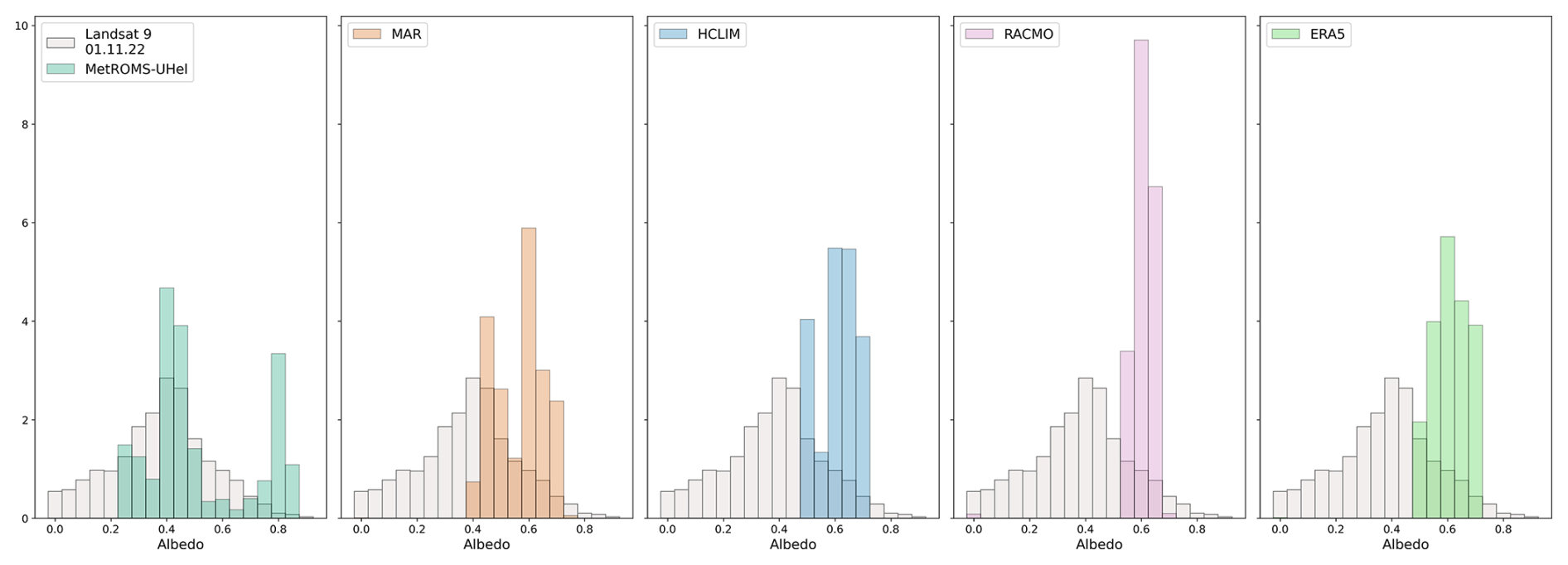
Because of the small area of the sea ice in the satellite images, more quantitative comparisons are difficult. Figure 10 shows the probability distributions for the sea ice albedo on the Landsat 9 image (Fig. 8), highlighting model deficiencies over the limited sample area. The surface albedo over the ocean/sea ice part of the Landsat 9 image has a wide distribution between 0 (open ocean) and 0.9 (snow-covered sea ice) and a clear maximum at 0.4. The regional climate models, particularly MAR with its low spatial resolution, lack detailed representation of the observed surface albedo. RACMO, ERA5, and HCLIM have a narrow distribution of sea ice albedo values, between the 0.4–0.75 range. Although HCLIM operates at a high, 2.5 km resolution, its sea surface temperature and sea-ice-concentration fields are derived from the 0.25° (∼28 km) resolution ERA5 reanalysis. As a result, any high-resolution sea ice variables output by HCLIM are influenced by the lower-resolution ERA5 forcing. The same is true for RACMO and MAR.

Among the tested models, MetROMS-UHel displays the largest variation in sea ice albedo over the same area covered by the satellite albedo products. The distribution of the modelled sea ice albedo is bimodal. Over this small sea ice area, the sea ice concentration in the model remains generally high (above 90 %). The fractional snow cover on top of the sea ice is also a key factor in determining sea ice albedo. The combination of high sea ice concentration (>95 %) and snow fraction (>90 %) in McMurdo Sound resembles the features of land-fast sea ice observed in the satellite images. This results in the high albedo peak centred at 0.8 in the MetROMS-UHel albedo distribution. However, unlike the Landsat 9 image, the MetROMS-UHel output fails to capture the distinct characteristics of free-floating sea ice both spatially and in its probability distribution. The MetROMS-UHel sea ice albedo distribution exhibits a lower albedo peak centred at 0.4, but albedos below 0.3 are not represented.

Model comparisons with such high-resolution, albeit limited-area, satellite products are valuable and should be further explored, ideally using larger satellite image datasets. These comparisons reveal the complexities of observed sea ice, highlighting model deficiencies while guiding advancements in model development.

4.6 Spatial albedo variability over the Weddell and Ross seas

The largest area of comparison is the Weddell (2 799 169 km²) and Ross seas (3 200 661 km²), defined by the size of the HCLIM respective domains. The maps for the satellite images, the model, and ERA5 over the Weddell Sea and Ross Sea are shown in Figs. 11 and 12. The distributions of the surface albedo over these areas are shown in Figs. 13 and 14. Furthermore, similar distributions but for sea ice and snow only (with fractional ocean albedo removed) are shown in Figs. B1 and B2 in Appendix B, illustrating the snow and ice albedo parameterisation distribution, without sea-ice-concentration effects.

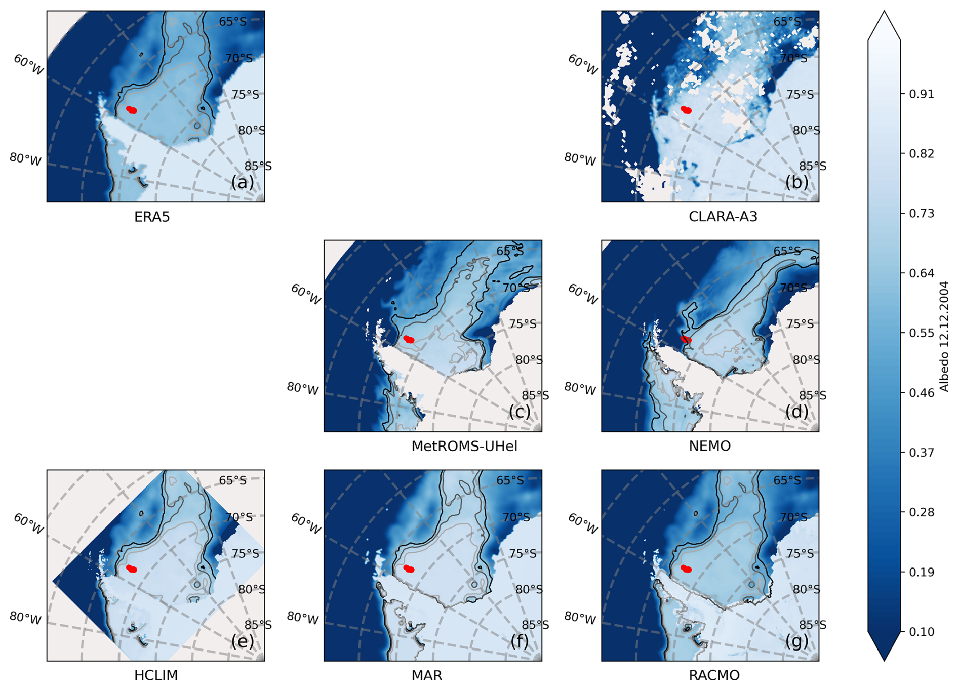
Figure 11 Monthly mean ERA5 (a) reanalysis and CLARA-A3 (b) satellite albedo products from over the Weddell Sea domain as reference for model validation and corresponding monthly mean albedo maps from MetROMS-UHel (c), NEMO (d), HCLIM (e), MAR (f), and RACMO (g) models. Sea ice concentration contours are shown on top with black, grey, and light-grey contour lines for the values of 0.7, 0.8, and 0.9 respectively. The location of the ISPOL field campaign is marked with red.

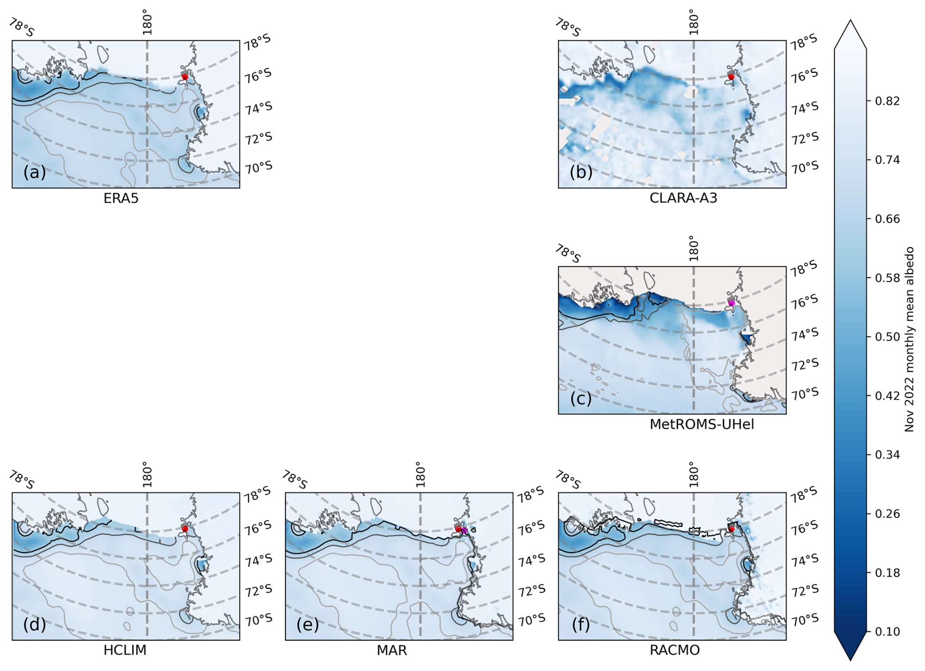
Figure 12 Monthly mean ERA5 reanalysis (a) and CLARA-A3 satellite albedo (b) products over the Ross Sea domain as reference for model validation and corresponding monthly mean albedo maps from MetROMS-UHel (c), HCLIM (d), MAR (e), and RACMO (f) models. Sea ice concentration contours are shown on top with black, grey, and light-grey contour lines for the values of 0.7, 0.8, and 0.9 respectively. The location of the ISPOL field campaign is marked with red. NEMO model runs are only available for the ISPOL case and not for the Marsden field campaign.

The surface albedo in the sea ice zone is always strongly influenced by sea ice concentration. HCLIM, MAR, and RACMO use the sea-ice-concentration fields from ERA5, which itself is satellite-derived. The spatial surface albedo patterns in Fig. 11 are therefore the same in these models. However, RACMO and ERA5 have lower sea ice albedo compared to CLARA-A3 and other models. This is better revealed in Fig. 13. The sea ice zone albedo in ERA5 has the first mode at 0.60, although the maximum observed sea ice zone albedo is as high as 0.85. The secondary mode of 0.05 is from points with no sea ice cover. RACMO has the first mode at 0.65. Figure B1 shows that sea-ice-concentration-independent snow and ice parameterisation over the whole region is about 0.65 for both ERA5 and RACMO. This value is consistent with Ebert and Curry (1993, Fig. 6, with Antarctic values shifted by 6 months), which shows sea ice albedo over Antarctica in mid-December to be around 0.6–0.7.

The regional oceanic models differ in the sea-ice-concentration patterns. We note that NEMO predicts the sea ice margin to be close to the ISPOL field campaign site. NEMO also has the first mode lower than expected from the observations, at 0.70, and does not describe 0.80 and higher albedo values due to overall lower sea ice concentrations. Figure B1 shows that the first mode for snow and ice albedo is at 0.80. Therefore, the main difference in the surface albedo comes from sea ice concentrations in NEMO and MetROMS-UHel, not from their albedo parameterisations. MetROMS-UHel model shows the best agreement with the spatial distribution and density distribution of the CLARA-A3 satellite albedo.

Over the Ross Sea domain, shown in Fig. 12, the albedo spatial pattern is a combination of sea ice concentration and snow fraction. The sea ice concentrations in the defined domain are mostly high, and we see only open water at the Ross Sea polynya. The CLARA-A3 image shows more small-scale variability, but the distribution shows a clear mode at 0.75–0.80. The models predict it correctly but do not describe the variety of lower, 0.2–0.7 albedo values. Exceptions are the ERA5, with a lower-than-observed strong mode at 0.7, and MetROMS-UHel, which matches the distribution of observed albedo values well. Notably, MetROMS-UHel reproduces the coastal polynya in front of the Ross Ice Shelf that can be seen from CLARA-A3 in Fig. 12.

RACMO does better over the Ross Sea in November 2004 than over the Weddell Sea in December 2004. When interpolating between monthly climatological averages in the sea ice albedo parameterisation of Ebert and Curry (1993), the predictions are occasionally accurate. The regional climate models MAR, HCLIM, and RACMO have similar behaviour over the Ross Sea, although RACMO has slightly lower first-mode snow albedo. The small differences come from parameterisations only, as the sea-ice-concentration fields are all the same ERA5 input.

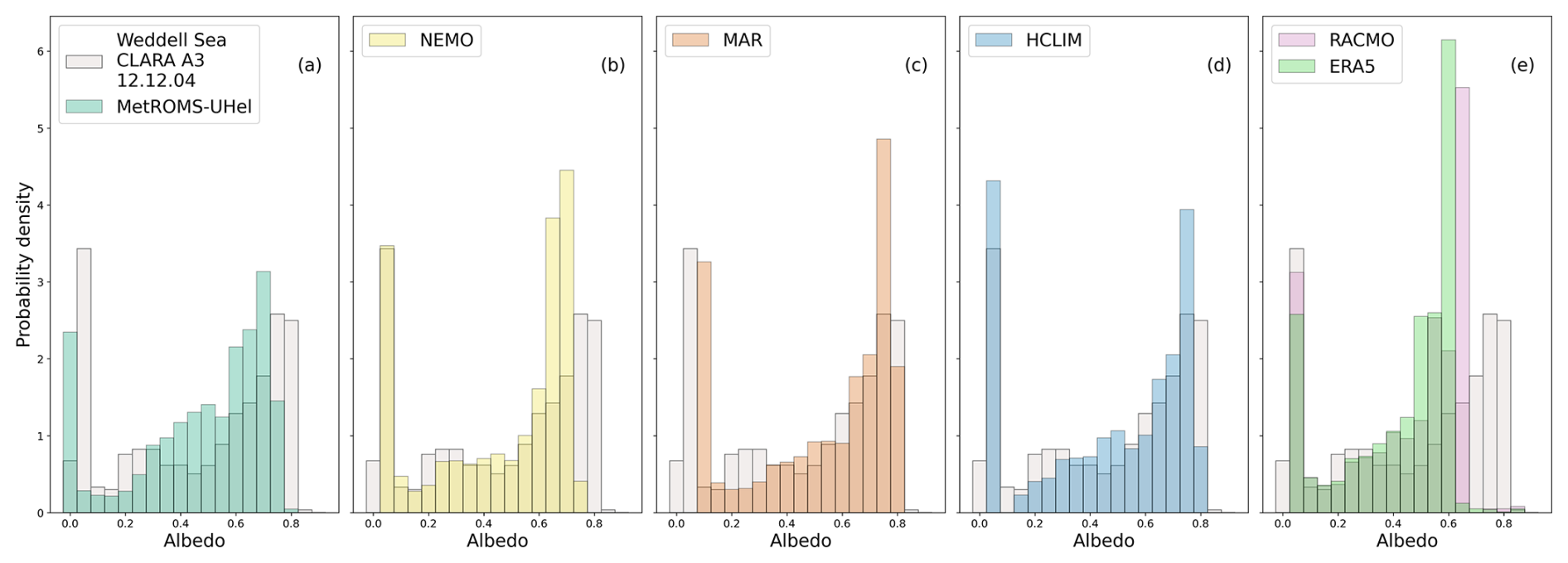
Figure 13 (a–e) December 2004 monthly average sea ice albedo distribution over a 2 799 169 km² Weddell Sea area (the area is defined by the smallest HCLIM domain size).

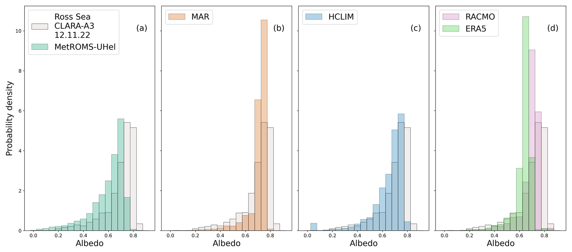
Figure 14 December 2004 monthly average sea ice albedo distribution of sea ice albedo over a 3 200 661 km² Ross Sea area (the area is defined by the smallest HCLIM domain size). NEMO model runs are only available for the ISPOL case and not for the Marsden field campaign.

5 Conclusions

This model comparison study examined the sea ice representation in three regional atmospheric models (HCLIM, MAR, RACMO), ERA5 reanalysis, and two regional ocean models (MetROMS-UHel, NEMO). We concentrated on sea ice albedo as described in Sect. 3. Each of the models used in this study is different in how they handle sea ice and surface albedo. We tested the models against various observational data – from detailed in situ data from the ISPOL and Marsden field campaigns, to small-area Landsat 9 and Sentinel 2 albedo products, to large-scale CLARA-A3 products. The regional atmospheric and ocean models rely on sea ice albedo parameterisations. However, due to the scarcity of observational data, especially over Antarctica, and the limitations imposed by model resolution and computational costs, simplified snow and ice albedo parameterisations are applied. The level of accuracy representing the ice and snow albedo required depends on the specific use case of a particular model, but even small adjustments in snow and ice albedo parameterisations can lead to significant improvements in reproducing the observed sea ice albedo, as well as other variables, such as surface temperatures. The key takeaways from our study are as follows:

1. Accurate parameterisation of bare ice and snow albedo is essential for model performance. Fine-tuning these parameters can enhance the model's ability to reproduce observed conditions. For example, initial tests with the HCLIM model revealed a significant warm bias in surface temperatures, with discrepancies as large as 5°C over sea ice compared to measurements from the ISPOL campaign. This bias was attributed to snow grain size distribution unsuitable for polar regions, which also led to modelled albedo that is too low. Updating the snow grain size distribution led to albedo levels similar to observations and removed the warm bias. Furthermore, ERA5 (and RACMO) uses time-interpolated monthly albedo values based on Ebert and Curry (1993), which has been identified as a limitation in this study and several other studies (Pohl et al., 2020; Müller et al., 2024; Batrak et al., 2024). RACMO and ERA5 predict significantly lower albedo sea ice over the Weddell Sea during the ISPOL campaign, 0.69 and 0.63, respectively, compared to the observed 0.78/0.82 at the ISPOL radiation measurement sites. This discrepancy extends across the entire Weddell Sea when compared to satellite data.

2. In drier sea ice regions like the Ross Sea, the key issue affecting the performance of albedo models is the treatment of fractional snow cover. When models simulate a fully snow-covered surface, their albedo values tend to be significantly higher than the observed albedo values, which incorporate substantial areas of snow-free sea ice. All models, except RACMO, predict high sea ice albedo in the range of 0.82 to 0.85, compared to the observed 0.79, due to their representation of uniform snow cover.

3. Sea surface albedo can be influenced by highly localised factors such as small-scale variations in sea ice concentration and patchy or blowing snow. As a result, higher-resolution models do not necessarily outperform lower-resolution models if these localised effects are not accounted for. For instance, although HCLIM operates at a 2.5 km spatial resolution, its sea-ice-concentration fields are derived from the 0.25° (∼28 km) resolution ERA5 data, and it employs a simple one-dimensional thermodynamic sea ice parameterisation scheme, which limits its ability to capture these finer-scale processes. The Landsat 9 high-resolution surface albedo image of the McMurdo Sound area shows a wide distribution ranging from 0 (open ocean) to 0.9 (snow-covered sea ice), with a clear peak at 0.4. In contrast, the regional models, both the low-resolution MAR and the high-resolution HCLIM, exhibit a narrow range of albedo values and fail to capture the detailed variability observed in the satellite data.

4. Comparing the modelled total (ice, snow and ocean) grid-box-averaged sea ice albedo to in situ measurements near the margins of the sea ice extent (with lower sea ice concentrations) or on land-fast sea ice (with highest sea ice concentrations) is problematic. In this study, HCLIM, MAR, and RACMO all used ERA5 sea-ice-concentration fields, but MetROMS-UHel and NEMO calculate these fields prognostically. For instance, the ISPOL campaign site was at the very margins of NEMO's sea ice extent. Furthermore, the location of the Marsden campaign site was complicated to the models – ERA5 and MAR consider the Marsden CS to be on land, not on sea ice. When evaluating ERA5 and MAR albedo during the Marsden campaign, the values from the closest sea ice grid point were used. Since HCLIM, MAR, and RACMO use sea ice concentrations from ERA5, it implies that these models extrapolate the sea ice concentrations to areas classified as land in ERA5.

Surface albedo over polar sea ice is complex, and this study focused only on first-order effects, excluding factors such as the cloud and solar zenith angle dependence of surface albedo, which themselves can be 10 % (Key et al., 2001; Gardner and Sharp, 2010; Jäkel et al., 2024). In case studies characterised by significant variation in surface types, such as during the spring/summer season, it is primarily uncertainties in the parameterisation of these surface types that influence the modelled surface albedo, rather than cloud effects (Jäkel et al., 2024). The effect of using different surface types can lead to a 20 %–30 % difference in albedo, such as when shifting from bare ice to snow-covered ice, as seen in the case of MAR (Fig. 4b). Using a snow albedo parameterisation that is not suitable for polar regions can result in differences exceeding 30 %, as demonstrated by HCLIM (Fig. 2). While future research should include a more comprehensive evaluation of cloud impacts, as explored by Jäkel et al. (2024) and Foth et al. (2024), there is still room for improvement by refining the aspects of albedo discussed in this paper. Coupling advanced radiative transfer models with regional climate or ocean models, as demonstrated in RACMO (though limited to land not sea ice), MetROMS-UHel, and SNICAR-ADv4 (Whicker et al., 2022), represents a major step forward in simulating surface processes. This approach enables a detailed representation of the optical properties of both snow and ice, thereby enhancing the accuracy and performance of coupled model systems.

Appendix A: Meteorological comparison extended

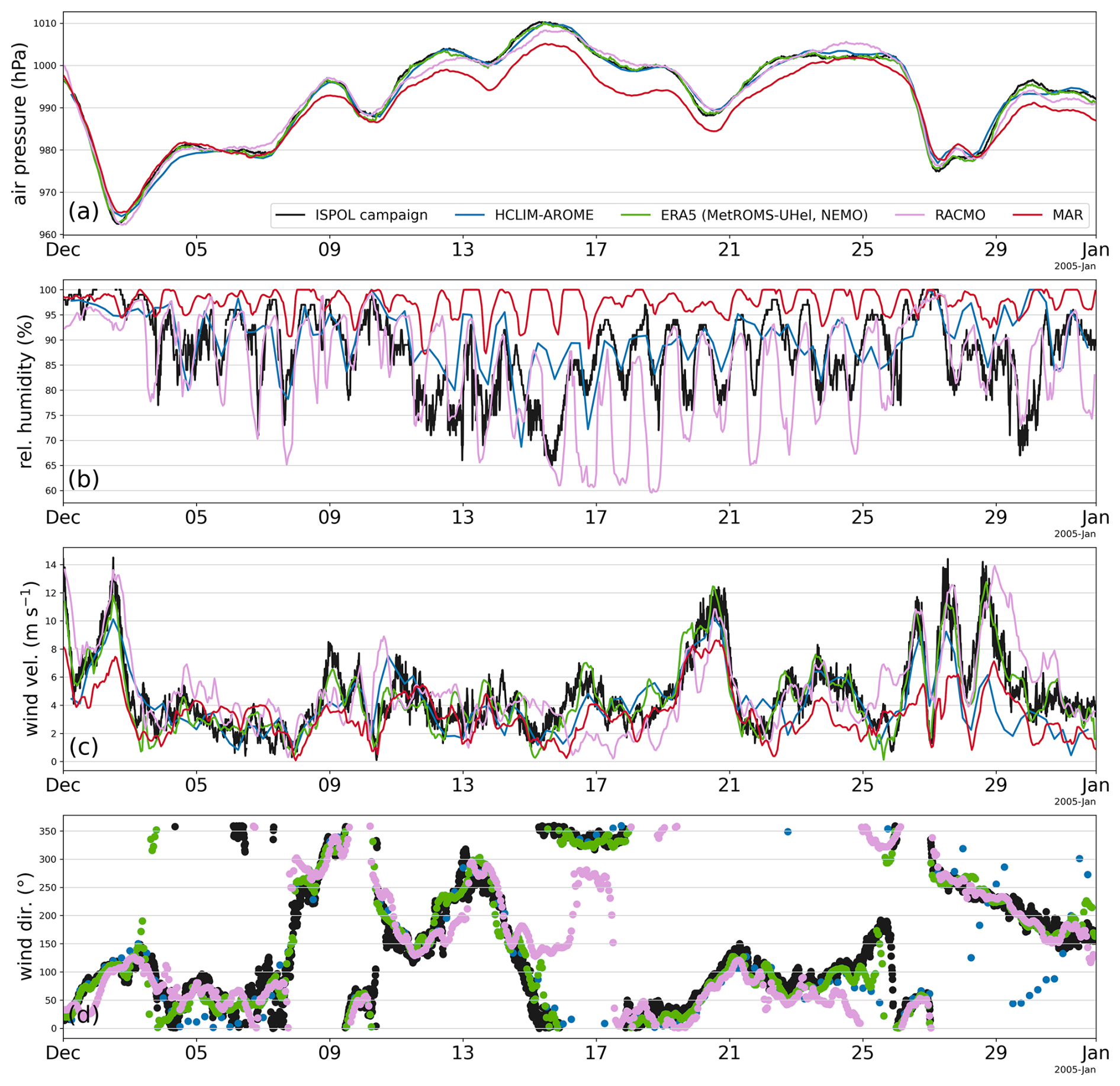
Figure A1 Weather conditions during the ISPOL experiment measured at the RV Polarstern (black) compared with the model output from HCLIM (blue), RACMO (pink), MAR (red), and ERA5 reanalysis (green). (a) Air pressure, (b) relative humidity, and (c, d) wind velocity and direction.

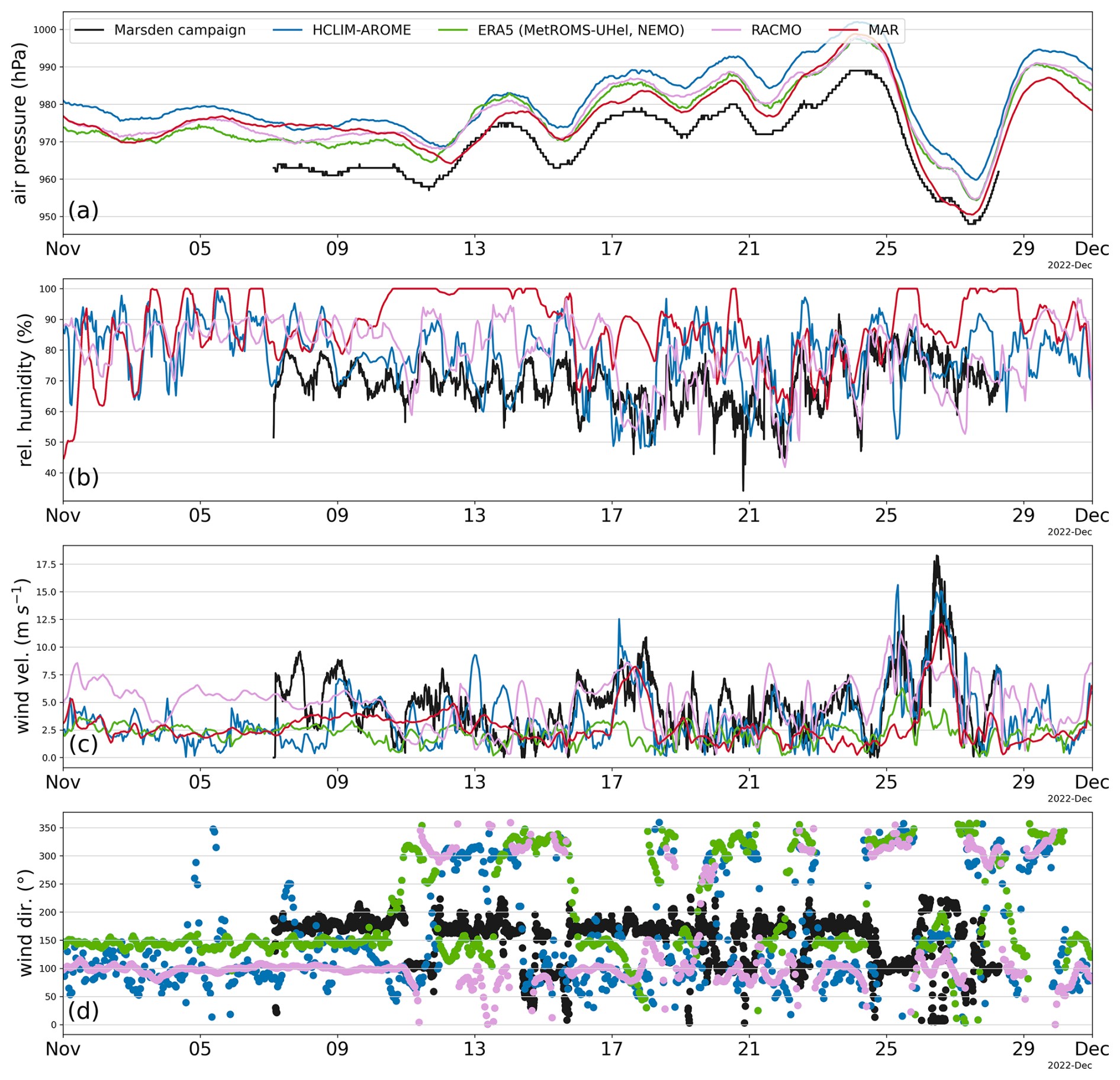
Figure A2 Weather conditions during the Marsden campaign compared with the model output from HCLIM (blue), RACMO (pink), MAR (red), and ERA5 reanalysis (green). (a) Air pressure, (b) relative humidity, and (c, d) wind velocity and direction.

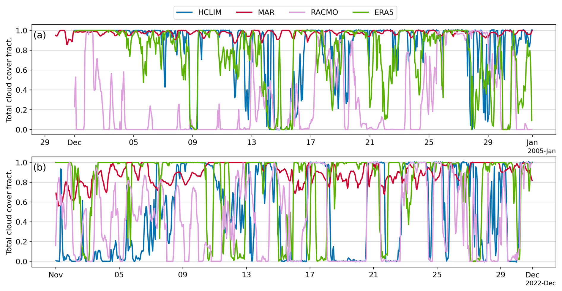
Figure A3 The modelled total cloud cover from HCLIM (blue), RACMO (pink), MAR (red), and ERA5 reanalysis (green).

Appendix B: Sea ice albedo distributions over Weddell and Ross seas, modelled snow and ice only

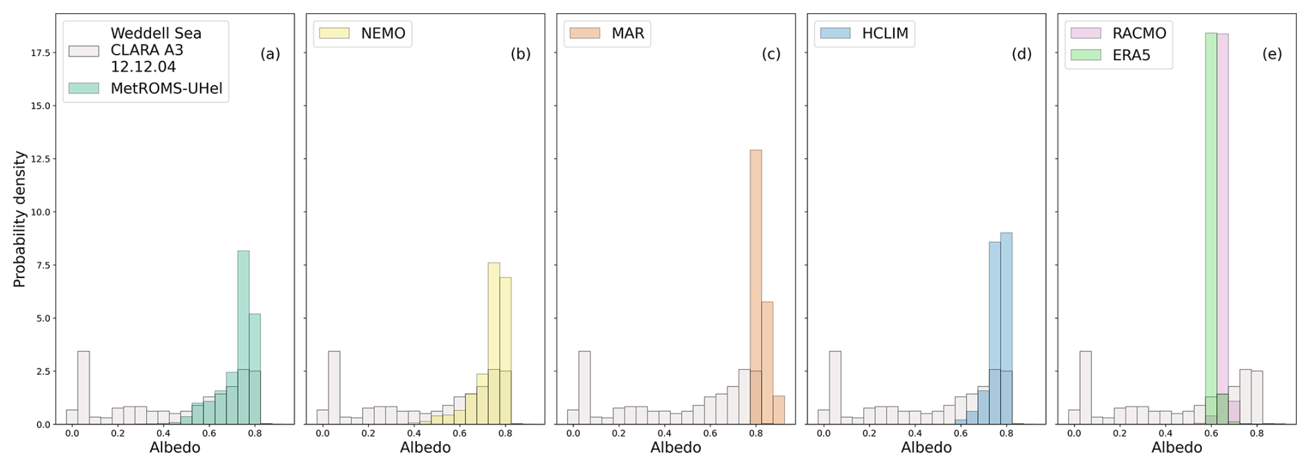
Figure B1 Probability distributions of monthly averaged sea ice albedo over a 2 799 169 km² Weddell Sea area (the area is defined by the smallest HCLIM domain size). For the model output in panels (a)–(e), only the contributions from sea ice and snow are shown, with ocean albedo removed.

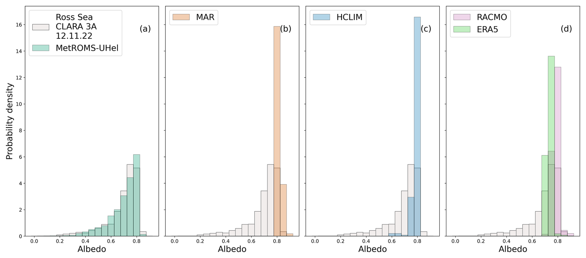
Figure B2 Probability distributions of monthly averaged sea ice albedo over a 3 200 661 km² Ross Sea area (defined by HCLIM domain size). For the model output in panels (a)–(d), only the contributions from sea ice and snow are shown, with ocean albedo removed. NEMO model runs are only available for the ISPOL case and not for the Marsden field campaign.