Multi-frequency altimetry snow depth estimates over heterogeneous snow-covered Antarctic summer sea ice – Part 2: Comparing airborne estimates with near-coincident CryoSat-2 and ICESat-2 (CRYO2ICE)

For the first time, a comparison of altimetry-derived snow depth estimates between dual-frequency spaceborne and near-coincident multi-frequency airborne estimates is conducted using data from the recent under-flight of a CryoSat-2 and ICESat-2 (CRYO2ICE) orbit by a simultaneous airborne campaign over the Weddell Sea in December 2022 carrying Ka-, Ku-, $\mathrm{C}/\mathrm{S}$-band radars and a scanning near-infrared lidar. From this unique combination of airborne sensors, the accuracy of snow depth captured by the near-coincident CRYO2ICE orbits can be evaluated. The CRYO2ICE snow depth achieved along the orbit was, on average, 0.34 m, which is within 0.01 m from passive-microwave-derived observations and 0.12 m from a model-based estimate. The retrieval methodology appears to play a significant role, which we suspect is highly dependent on the classification and filtration schemes applied to remove potentially ambiguous altimetry observations. Comparison with airborne snow depths at 25 km segments showed correlations of 0.51–0.53, a bias of 0.03 m, and root-mean-square deviation of 0.08 m when using the airborne lidar scanner as air–snow interface and $\mathrm{C}/\mathrm{S}$-band at maximum amplitude at the snow–ice interface. To understand how comparisons across ground, air, and space shall be conducted, especially in preparation for the upcoming dual-frequency radar altimeter mission Copernicus Polar Ice and Snow Topography Altimeter (CRISTAL), it is critical that we investigate the impact of different scattering mechanisms at varying frequencies for diverging viewing geometries considering dissimilar spatial and range resolutions.

1 Introduction

With its insulating properties and its regulating role in sea ice growth and melt, snow on sea ice plays a pivotal role in the climate system (Webster et al., 2018; Sturm et al., 2002). Snow is considered a key component in the sea ice thickness retrieval methodology using satellite altimetry under the assumption of hydrostatic equilibrium; thus, it is critical that accurate and timely large-scale estimates of snow depth are available. For Antarctic sea ice, this is especially critical considering the multi-layered, complex, and heterogeneous snow cover present due to the relatively warm air temperature coupled with strong winds, heavy precipitation, and relatively thin ice (Massom et al., 2001). Such exceptional conditions result in significant snow metamorphism occurring, limiting microwave radar penetration into snow and further complicating the radar signals observed. The relatively warm temperatures can enlarge snow grain sizes, create internal ice layers, and ensure the presence of liquid water within the snowpack (Webster et al., 2018). Considering the predominantly seasonal and relatively thin ice cover (Worby et al., 2008), capillary brine wicking into the basal snow layer and increasing salinity of the snow cover can further limit microwave penetration (Nandan et al., 2017). These conditions permit the survival of a year-round, highly complex, and diversified snow cover (Arndt and Paul, 2018).

Recent studies (e.g., Garnier et al., 2021; Lawrence et al., 2018; Kwok and Maksym, 2014; Kacimi and Kwok, 2022) have utilised dual-frequency or multiple-interface-tracing approaches to derive snow depth from altimetry by using a measure of the air–snow (a-s) and snow–ice (s-i) interfaces. Frequently, the a-s interface has been observed using laser observations that reflect at (or very close to) the snow surface (Kacimi and Kwok, 2022, 2020), where freeboard (elevation of ice above local water level) observations computed from lasers are referred to as the total freeboard (snow + ice). Since its launch in 2014, observations from a high-frequency satellite radar altimeter operating at Ka-band have also been used as a measure of a-s interface based on the assumption of limited penetration into snow (Garnier et al., 2021; Guerreiro et al., 2016). The s-i interface has usually been observed by use of Ku-band radars, where laboratory experiments have shown that Ku-band signals can penetrate to the s-i interface under cold and dry conditions (Beaven et al., 1995). Thus, Ku-band observations are generally assumed to penetrate the snow cover, hence providing radar freeboards which, when corrected for slower wave propagation speed, are converted to sea ice freeboards (e.g., Hendricks, 2022; Mallett et al., 2020). However, this assumption has been disputed in several studies (e.g., Nab et al., 2023; Willatt et al., 2023, 2010, 2011; De Rijke-Thomas et al., 2023; Armitage and Ridout, 2015; Rösel et al., 2021; King et al., 2018; Nandan et al., 2017, 2020, 2023) based on data from ground-based, airborne, and spaceborne observations. Here, they argued that phenomena such as snow metamorphism, redistribution, brine wicking, or flooding can significantly limit the penetration of Ku-band waves. However, even based on observations showing that Ku-band penetration can be limited, the dual-frequency approach remains one of the few Earth observation methods expected to observe snow depth over sea ice under optimal conditions. These assumptions are pivotal for the future dual-frequency $\mathrm{Ka}/\mathrm{Ku}$-band polar radar altimetry mission Copernicus Polar Ice and Snow Topography Altimeter (CRISTAL), planned for launch in 2027/2028 (Kern et al., 2020), where the dual-frequency approach is one of the driving factors of the satellite design. To investigate the simultaneous dual-frequency approach further, ESA altered the orbit of their polar Ku-band radar altimetry mission, i.e., CryoSat-2, in July 2020 to align periodically with NASA's polar laser altimetry mission, i.e., the Ice, Cloud, and land Elevation Satellite-2 (ICESat-2), for the Northern Hemisphere, known as the CRYO2ICE Resonance Campaign. This alignment was further adjusted in July 2022 to maximise orbits in the Southern Hemisphere.

Currently, spaceborne dual-frequency altimetry for snow depth estimation has been relatively widely used in the Arctic (e.g., Lawrence et al., 2018; Guerreiro et al., 2016; Garnier et al., 2021; Kacimi and Kwok, 2020; Fredensborg Hansen et al., 2024a), with few attempts to apply it in the Antarctic (e.g., Kacimi and Kwok, 2022; Garnier et al., 2021) due to the challenging snow conditions. Furthermore, most studies on satellite altimetry dual-frequency approaches rely on monthly-based, gridded snow depth composites rather than orbit-wise estimates. Fredensborg Hansen et al. (2024a) presented the first estimates of satellite-derived dual-frequency snow depth along orbits; however, a direct validation of these observations was limited to a few in situ buoys available. Fortunately, in December 2022, the CryoSat Validation Experiment (CryoVEx) programme with ESA in collaboration with the Natural Environment Research Council (NERC) Drivers and Effects of Fluctuations in sea Ice in the ANTarctic (DEFIANT) project completed an airborne campaign over Antarctic land and sea ice. There, an under-flight was performed for a CRYO2ICE orbit on 13 December 2022, carrying a full suite of instruments relevant for estimating snow depth over sea ice and evaluating microwave penetration with the use of different sensors, including $\mathrm{C}/\mathrm{S}$- (“snow radar”), Ka-, and Ku-band radar altimeters. This campaign presents the first opportunity to compare near-coincident dual-frequency satellite-derived snow depth estimates with simultaneous airborne snow depth estimates derived from multi-frequency approaches.

Here, we present the second part of a two-part study, where we compare airborne snow depth estimates derived from the traditional hypothesis of microwave penetration into snow (Part 1; see Fredensborg Hansen et al., 2025; hereafter cited as Part 1) with near-coincident spaceborne radar (CryoSat-2) and laser (ICESat-2) orbits along a dedicated CRYO2ICE orbit. This is currently the only CRYO2ICE (or any dual-frequency satellite orbit) validation under-flight carried out with a full suite of instruments able to evaluate penetration into the snow. In particular, this study aims to evaluate the capabilities of CRYO2ICE (emulating the future CRISTAL dual-frequency polar satellite altimetry mission) to estimate snow depth along-track similar to what the airborne sensors observe. Of particular interest is the unique combination of airborne sensors (at $\mathrm{C}/\mathrm{S}$-band, Ku-band, and Ka-band) from which different information on the snow conditions might be leveraged.

2 Data

2.1 ICESat-2 and CryoSat-2 (CRYO2ICE)

2.1.1 ICESat-2

ICESat-2 carries a photon-counting Advanced Topographic Laser Altimeter System (ATLAS) that transmits green laser pulses (532 nm) split into a six-beam measurement configuration separated into three beam pairs (gt1–3). Each beam pair carries a strong and a weak beam, and they are denoted as left (gtl) or right (gtr) beams relative to the satellite orientation (Neumann et al., 2019). For this particular track, the ICESat-2 spacecraft was in forward orientation, which resulted in gtl beams being designated as strong beams and gtr as weak. Each laser pulse is emitted with a pulse repetition frequency of 10 kHz, leading to a 0.7 m along-track separation that, with a footprint of 11–17 m at nominal altitude (Magruder et al., 2020), allows for oversampling and unprecedented surface sampling. The operational Sea Ice Heights product (ATL07, Kwok et al., 2023a) aggregates 150 photons into surface segments and identifies the segments as floes or leads based on a radiometric classification. These 150-photon aggregates result in inconsistent segment lengths based on surface reflectivity and specularity. From ATL07, along-track freeboards are calculated in the ATL10 product based on a reference sea ice surface derived from the available lead (or sea surface height) segments. For ATL10 (Kwok et al., 2023b), a sea surface height reference is provided for consecutive 10 km along-track sections where at least one sea surface sample (lead) is available for each beam independently. Hereafter, the sea surface height segment elevation is subtracted from the floe heights to provide total freeboards. Negative total freeboards are set to 0. For this study, data from ATL07 and ATL10 release 006 (r006) are used. ATL07 is used only for visualisation purposes, whereas ATL10 is used for processing. ICESat-2 is sensitive to the presence of clouds and fog, altering the location of the reflection interface due to limited penetration, resulting in gaps along the track (e.g., Fredensborg Hansen et al., 2021; Petty et al., 2021).

2.1.2 CryoSat-2

CryoSat-2 carries the interferometric Ku-band synthetic aperture radar (SAR) altimeter (SIRAL), which primarily acquires observations in SAR mode over sea ice. In SAR mode, the radar waveform is computed through delay-Doppler SAR processing of 64 individual bursts, which are multi-looked to provide a waveform for each Doppler beam with a footprint of ∼ 300 × 1650 m sampled at 20 kHz (Scagliola, 2013). Due to the various processing chains used to derive radar freeboards from CryoSat-2, we introduce three different products used to evaluate the sensitivity of different retrieval methods. While different geophysical corrections might be applied across the various freeboard products, we do not assume these to play a significant role, since freeboards are relative observations and since the impact is of the order of centimetres, primarily related to lead-sparse areas (Ricker et al., 2016). The processing chains and products are briefly described below. For all products, the radar freeboard is derived by differencing an interpolated sea level anomaly, using observations classified as leads as tie-points, from the observations classified as originating from ice floes.

• ESA Baseline-E (ESA-E). The operational ESA-E observations in SAR mode provide radar freeboard by a combined waveform retracker. For diffuse waveforms, which are expected to originate from floes, a 70 % threshold first-maximum retracker algorithm (TFMRA) is applied, and for specular echoes (i.e., leads) a peak-finder based on the model-fitting method described in Giles et al. (2007) is implemented. Leads and floes are discriminated based on a combination of parameters including sea ice concentration, waveform peakiness, standard deviation of the stack of waveforms, and peakiness of the stack (Meloni et al., 2020), following methods presented in Passaro et al. (2018). ESA-E radar freeboards used here are pre-processed following the methodology presented in Fredensborg Hansen et al. (2024a, their Supporting Information S1) to remove erroneous observations.

• ESA CryoSat ThEMatic PrOducts (CryoTEMPO) over sea ice. The CryoTEMPO products aim to deliver simplified, harmonised, and agile CryoSat-2 products that are easily accessible and usable by non-altimeter experts and end-users with the possibility of evolving the processing chain depending on the current state of the art. The CryoTEMPO sea ice thematic product (Hendricks, 2022) contains geolocated and time-associated radar freeboards and sea ice freeboards with associated uncertainties. The surface elevations are derived using the Sar Altimetry MOde Studies and Applications over ocean (SAMOSA+) algorithm with an unrestricted waveform classification, allowing for retrieval of freeboards over mixed surfaces and thinner floes (Stefan Hendricks, personal communication, 2024). The radar freeboard is converted to sea ice freeboard (not used in this study) with an outlier restriction of −0.25 to 2.25 m applied, where identified outliers are removed from both parameters for consistency. The reader is referred to Hendricks (2022) for further information.

• Fully focused SAR (FF-SAR). The FF-SAR technique performs the coherent processing of the radar echoes during the whole illumination time of a surface scatterer (Egido and Smith, 2017, 2019). This processing enhances surface resolution, enabling the discrimination of smaller features on the sea ice surface, potentially leading to improved freeboard estimation. Surface elevation information is retrieved from multi-looked FF-SAR waveforms with a physical sea ice retracker (Egido et al., 2022). Waveforms are classified as lead, floe, or ambiguous ice based on the specular versus diffuse power ratio (often denoted as SDR).

2.2 CRYO2ICEANT22 airborne campaign and sensors

With the continuation of the ESA validation programme CryoVEx under the Cryo2IceEx and NERC DEFIANT projects in December 2022, the first under-flight of a CRYO2ICE orbit carrying radars possible to evaluate microwave penetration was completed. This airborne campaign (dubbed CRYO2ICEANT22) captured a dedicated CRYO2ICE orbit over sea ice in the Weddell Sea on 13 December 2022. The full survey flight took place from 15:52 to 00:29 UTC (following day), with the satellite orbit under-flight occurring at ∼ 18:48–21:46 UTC, with ICESat-2 (orbit number 23676, reference ground track 1283) passing at ∼ 17:36 UTC and CryoSat-2 (absolute orbit number 67222) passing at ∼ 20:16 UTC. The airborne campaign was aligned with the CryoSat-2-predicted orbit, and all observations were within 60 m from the CryoSat-2 observations with ∼ 80 % within 20 m (not shown).

The surveys were carried out using a British Antarctic Survey (BAS) DASH-7 aircraft from Rothera Research Station with CReSIS Ka- (32–38 GHz), Ku- (12–18 GHz), and $\mathrm{C}/\mathrm{S}$-band (2–8 GHz) radar altimeters, as well as an airborne laser scanner (ALS) of the type Riegl LMS Q‐240i‐80. An in-depth description of the airborne sensors and associated data processing can be found in Fredensborg Hansen et al. (2025, Part 1). Briefly summarised, the Ku- and Ka-band radar altimeters are assumed to have a primary scattering from a single surface (assumed to be the snow–ice and air–snow interfaces, respectively), which are assumed to be trackable using the threshold first-maximum retracker algorithm (TFMRA). Here, different retracking thresholds (40 %, 50 %, or 80 %) are used to track different locations of the leading edge of the radar waveform which have commonly been used to best represent the “average” surface elevation within a footprint. The $\mathrm{C}/\mathrm{S}$-band radar (snow radar) is assumed to have scattering from both the air–snow and snow–ice interfaces, trackable from single waveforms. These interfaces are retrieved using two algorithms: continuous wavelet transform (CWT; Newman et al., 2014) or peakiness (PEAK; Jutila et al., 2022). For all three radars, the location of the maximum power (MAX) on the waveform is extracted to represent the dominant scattering interface. The swath available from ALS is used to extract a vertical nadir profile emulating the a-s interface at the location of the radars. This is achieved by averaging all ALS observations within a 5 m diameter footprint at each radar observation.

There was no in situ component carried out over sea ice; hence, ground-truth data describing the snow conditions are unavailable. We were also unable to identify other reference observations (e.g., buoys) available to provide input on the conditions.

2.3 Auxiliary data

Ideally, for the validation of snow depth derived from the airborne and spaceborne $\mathrm{Ka}/\mathrm{Ku}$ combinations, one would use the snow radar on board the same platform. However, the methodologies currently used to derive snow depth from snow radars have been validated primarily for the Arctic (Kwok et al., 2017a; Jutila et al., 2022; Kurtz and Farrell, 2011) or applied during winter conditions (October) in the Weddell Sea and Bellingshausen Sea (Kwok and Maksym, 2014; Kwok and Kacimi, 2018) for campaigns flown in 2010–2016, so they may not represent the sea ice conditions during this campaign. Therefore, we also compare the CRYO2ICE results with additional snow depth estimates (passive-microwave-derived or modelled).

2.3.1 AMSR2 passive-microwave radiometer-derived snow depth

We use the passive-microwave-derived snow depth product by (Meier et al., 2018). The snow depth estimate is derived from AMSR2 observations using the methodology of Markus and Cavalieri (1998) and is provided in a polar stereographic projection at a 12.5 km resolution as a daily estimate of a 5 d average. The same method is applied to both hemispheres but excludes perennial areas of the Arctic (Meier et al., 2018). The algorithm is only applicable to dry snow. Large temporal fluctuations can occur due to freeze–thaw events, where wet snow during the day refreezes during the night, resulting in large grain sizes. This, in turn, leads to reduced emissivity at higher frequencies, which can result in an overestimation of snow depth (Meier et al., 2018). For this study, we extract the nearest-neighbouring AMSR2 observations along the CRYO2ICE observations for comparison.

2.3.2 CASSIS snow depth

Centre for Polar Observation and Modelling (CPOM) Antarctic Snow on Sea Ice Simulation (CASSIS) simulates the daily creation and drift of floes, where the floes accumulate snow from the atmosphere and Antarctic Ice Sheet and lose snow to the ocean and snow-ice formation (Lawrence et al., 2024). Here, they utilise a Lagrangian framework to accumulate snow on top of floes while taking into account katabatic snowfall from ice shelves and snow-ice formation by assuming 55 % of the daily snow accumulation submerges and refreezes. The CASSIS model is provided at a daily resolution in a polar stereographic grid with a tangential plane at 70° S at 10 km grid resolution, and the Lagrangian points are initiated on the 21 February every year with ship-based observations collected within the Antarctic Sea-Ice Processes and Climate (ASPeCt) programme. We extract the nearest-neighbouring CASSIS observation along the CRYO2ICE observations for comparison.

3 Methodology

3.1 Collocation of CRYO2ICE observations

For the collocation of CryoSat-2 and ICESat-2 freeboard observations along a CRYO2ICE orbit, we follow the methodology presented in Fredensborg Hansen et al. (2024a). In summary, one uses the observed CryoSat-2 radar freeboards as the baseline for collocating ICESat-2 observations. Here, we compute this individually for all three processing chains of CryoSat-2 data (ESA-E, FF-SAR, and CryoTEMPO). All ICESat-2 total freeboard observations (from all three beam pairs including both strong and weak beams) within a search radius of 3.5 km from the observed CryoSat-2 radar freeboard are selected. An average inverse-distancing-weighted ICESat-2 total freeboard observation per CryoSat-2 radar freeboard is then computed. At each CryoSat-2 observation, smoothing is applied using the same search radius (analogous to a smoothing along-track window of 7 km) to reduce noise.

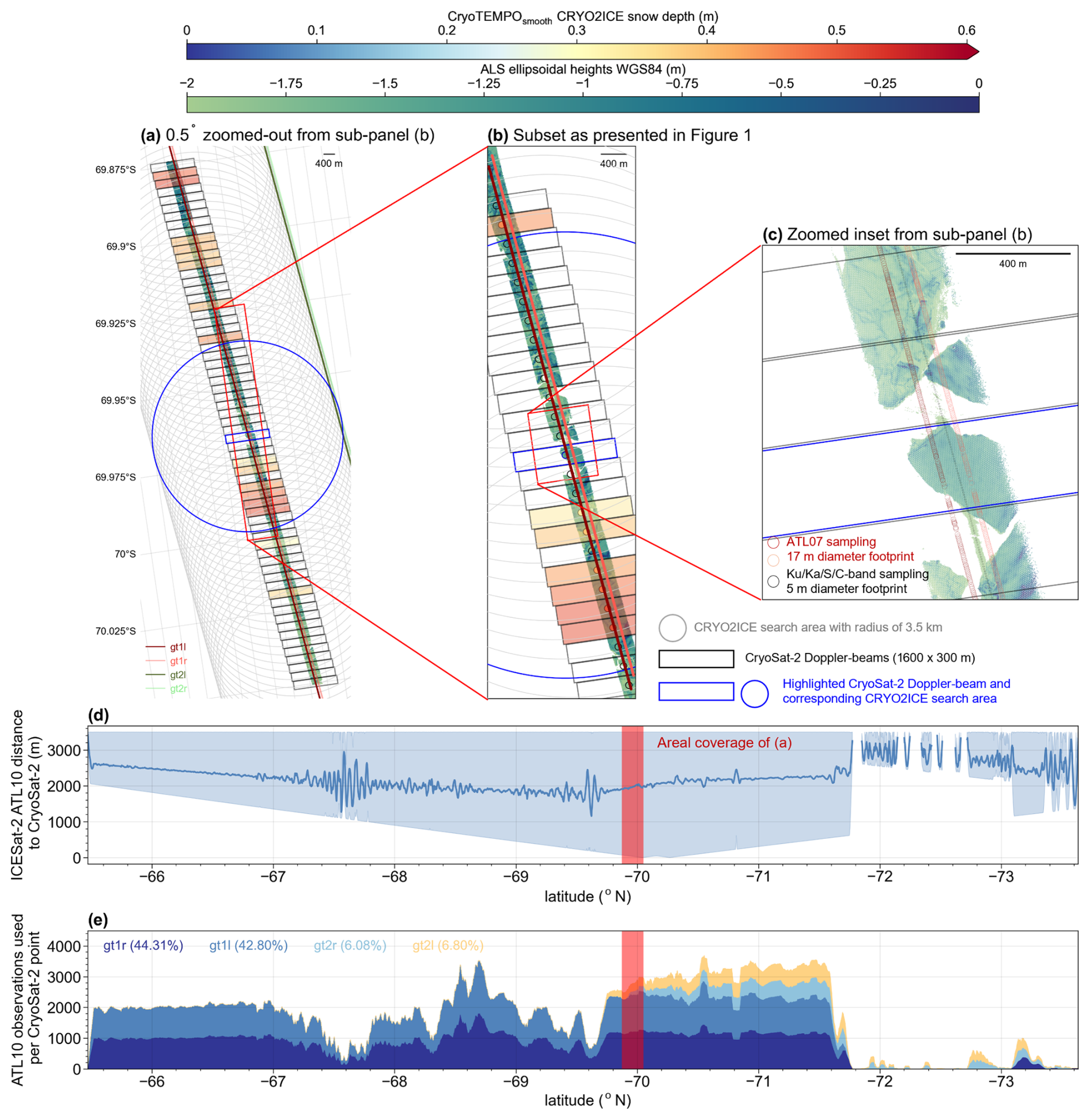
Figure 1 Comparison of data coverage between CryoSat-2, ICESat-2 (coinciding beams), and airborne data, and statistics of CRYO2ICE collocation. The CryoSat-2 Doppler beams are coloured according to the CRYO2ICE-derived snow depth when available. (a) Transect along the CRYO2ICEANT22 and CRYO2ICE under-flight (0.5° zoom-out from the subset shown in panel b) highlighting the full coverage of the 3.5 km search radius applied to CryoSat-2 and ICESat-2 observations for collocating CRYO2ICE observations, including ICESat-2 leftmost and central beam pairs. (b) A subset of the CRYO2ICEANT22 transect (for location, see Part 1), where, in addition to the CryoSat-2 Doppler-beam footprints, the central location of each Doppler-beam is shown by a small, not to scale, point-coloured according to the derived CRYO2ICE snow depth. (c) Further zoom into the subset highlights the footprint of ICESat-2, CryoSat-2 Doppler-beams, and the airborne observations. (d) Average distance to ICESat-2 ATL10 freeboard observations from each CryoSat-2 observation, where the shaded area denoted maximum and minimum distance. (e) The Number of ATL10 observations used per CryoSat-2 point to derive the CRYO2ICE ICESat-2 collocated total freeboard observations, separated per beam. The red vertical span on (d)–(e) presents the coverage presented in panel (a).

An example of the spatial scales to consider is presented in Fig. 1. Here, it is evident that ICESat-2 and CryoSat-2 are not fully aligned along the track, i.e., for this part the best alignment between ICESat-2 and CryoSat-2 occurs with the left beam pair (gt1r/l), which accounts for 87 % of CRYO2ICE observations along the entire track (Fig. 1e). Towards the pole, the remaining 13 % aligns with the centre beam pair. This is also illustrated in Fig. 1a, particularly in the northern part of the transect where the beams are positioned on the easternmost side of the ALS swath, whereas the opposite is the case at the southernmost part of the transect. In addition, it is clear that applying a 3.5 km search radius incorporates observations from neighbouring beam pairs when they are in the vicinity. Figure 1d shows the average distance between the closest ICESat-2 beam pair, and CryoSat-2 varies between ∼ 2000 and 3000 m with a minimum distance of less than 1 m, where the highest coincidence with one of the beams occur. Since a smoothing radius is applied, each CRYO2ICE ICESat-2-weighted average freeboard includes observations before and after the CryoSat-2 observation along the track (see also Fig. 1 for the spatial scales). The reader is referred to Fredensborg Hansen et al. (2024a) for further details and comparison over Arctic sea ice.

3.2 Snow depth retrieval from dual-frequency approaches

Similarly to former dual-frequency snow depth studies (e.g., Kwok et al., 2020; Lawrence et al., 2018; Garnier et al., 2021; Fredensborg Hansen et al., 2024a), snow depth is retrieved by differencing the height of the air–snow interface (total freeboard from laser) and the snow–ice interface (represented by Ku-band radar freeboard assuming full penetration) while accounting for the delay in radar wave propagation speed by use of the refractive index of snow considering its density. Here, we utilise a constant bulk density of snow of 300 kg m⁻³. The methodology is described in detail in Part 1.

3.3 Accounting for the spatial scales through smoothing and segmentation

For comparison with the CRYO2ICE spaceborne data, we first average the airborne observations into 1 km segments following the method presented in Jutila et al. (2022). These 1 km average segments are used to smooth the high-resolution spatial snow depth variability that cannot be obtained from the Doppler-beam footprints of CryoSat-2. From these 1 km segments, we further derive CRYO2ICE-comparable snow depths using the same along-track smoothing search radius of 3.5 km. In addition, we segment both the CRYO2ICE snow depths and the airborne counterparts into 25 km segments, following the approach of Garnier et al. (2021) and aligning with the CRISTAL requirements (Kern et al., 2020).

4 Results

4.1 Evaluation of radar and total freeboard along the CRYO2ICE orbit

First, it is important to note the number of observations removed from processing when computing freeboards. This processing includes removal of ambiguous data through surface classification, errors in surface retrieval, filtering by set thresholds, and distance to the closest leads. For example, ESA-E provides 3269 sea surface height (or ellipsoidal height) observations along the full track (where the surface has been identified as sea ice). In comparison, FF-SAR provides instead 10 785 observations. However, the individual processing chains applied to ESA-E, FF-SAR, and CryoTEMPO resulted in only 440, 286, and 2212 radar freeboard observations, respectively, considering only radar freeboards within 3 m of the water level. Of these, 29.77 %, 24.83 %, and 32.10 % of the observations, respectively, had radar freeboards below −0.1 m. Here, we remove freeboards below −0.1 m (as opposed to Fredensborg Hansen et al., 2024a, who kept all negative freeboards over Arctic sea ice), since they present a significant contribution to a smoothed CRYO2ICE CryoSat-2 freeboard (compared with their ∼ 5 % negative freeboards). This results in 309, 215, and 1502 radar freeboard observations for ESA-E, FF-SAR, and CryoTEMPO, respectively, to apply the smoothing window on (∼ 7 km, or search radius of 3.5 km following Fredensborg Hansen et al., 2024a). For further data processing, we consider only the filtered and smoothed CryoSat-2 products.

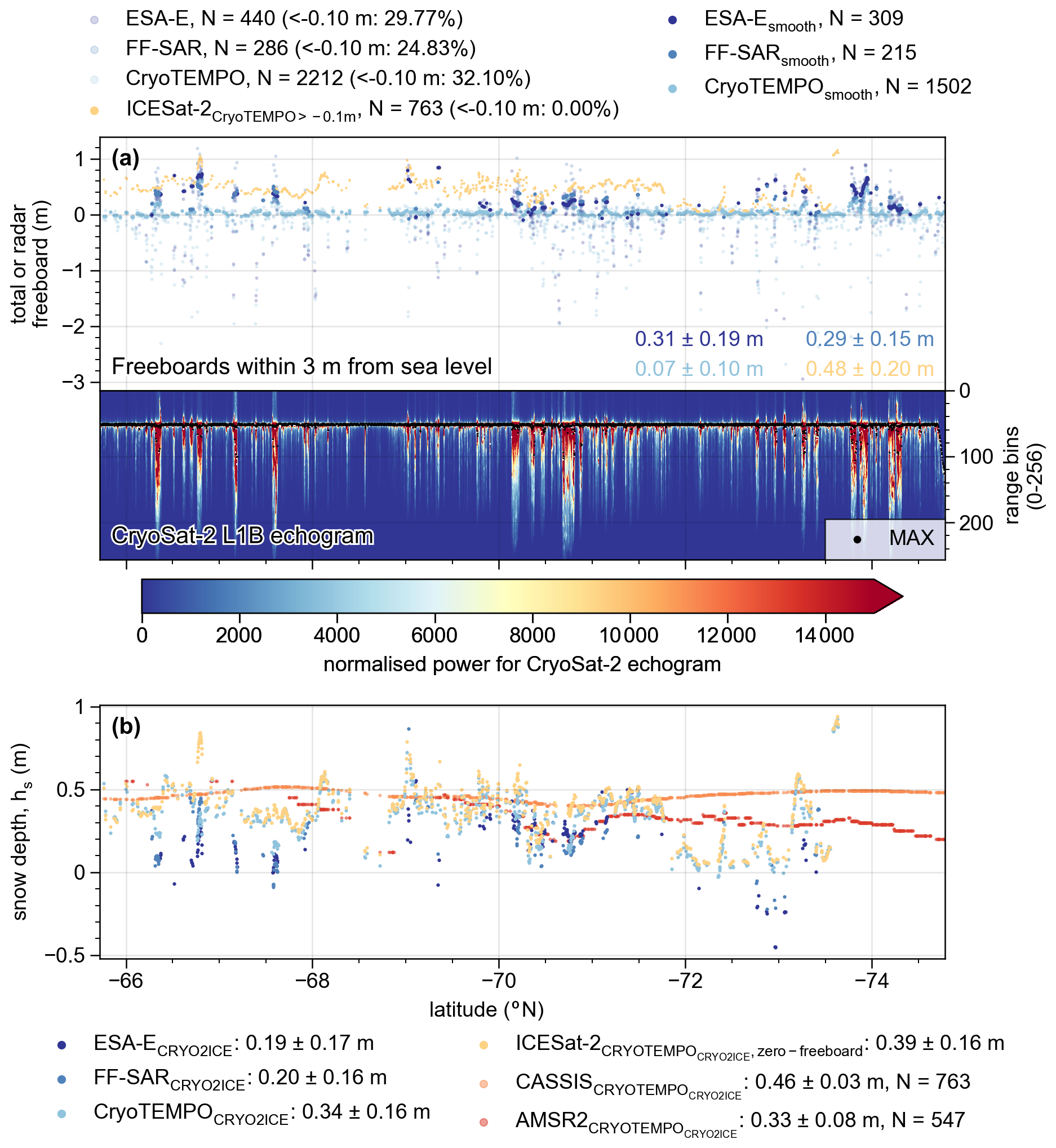
Figure 2 Estimation of snow depth along the CRYO2ICE orbit using CryoSat-2 radar freeboard observations from Baseline-E (ESA-E), fully focused SAR (FF-SAR), or the CryoTEMPO processing chains, as well as ICESat-2 ATL10 observations. (a) CryoSat-2 radar freeboards within 3 m from water level at native resolution, smoothed CryoSat-2 radar freeboards (using radar freeboards above −0.1 m), and total freeboard from ICESat-2 derived from smoothed CryoTEMPO observations following the methodology of Fredensborg Hansen et al. (2024a). In addition, the CryoSat-2 L1B echogram (radar waveforms) is provided to identify outliers in radar freeboards, where the colour bar shows the normalised power of the waveforms as available in the CryoSat-2 ESA-E product (normalised to 0–65,535 with the colour bar adjusted for visualisation purposes). (b) Derived snow depth is shown for each CryoSat-2 processing chain (smoothed) using derived ICESat-2 CRYO2ICE total freeboards and compared with nearest-neighbouring CASSIS and AMSR2 snow depths. Average and standard deviation are given for radar/total freeboards (for all available data points) and snow depth (whenever CRYO2ICE observations are available, and for CASSIS and AMSR2 snow depths, the statistics are provided along CryoTEMPO_CRYO2ICE). Note that the latitudinal extent of the CRYO2ICE only partly overlaps with the under-flight as shown here. In particular, AMSR2 observations are mostly available south of the airborne under-flight; see Part 1.

Comparing the freeboards along-track (Fig. 2), it is evident that both ESA-E and FF-SAR achieve similar results at the few points available along track (average of 0.31 ± 0.19 and 0.29 ± 0.15 m, respectively), whereas CryoTEMPO has significantly lower average radar freeboard (at 0.07 ± 0.1 m). Furthermore, CryoTEMPO provides significantly more observations than any of the other processing chains (>4 times). FF-SAR and ESA-E generally provide observations where mostly highly diffuse waveforms are present (see Fig. 2a), whereas CryoTEMPO is able to generate freeboards over less diffuse waveforms likely caused by thinner sea ice and/or a heterogeneous ice cover with significant dominance of specularity. This is probably due to the different surface classification schemes applied, where ESA-E and FF-SAR apply more strict requirements to their waveforms. This also explains the ability to extract much smaller freeboards (of, on average, 0.07 m and where 931 of the 1502 (or 62 %) filtered radar freeboard observations were below the average value, with 453 of these 931 observations being positive). CryoTEMPO's average radar freeboard ranges close to a zero-freeboard assumption (that the sea ice surface, where Ku-band under dry and cold conditions is reflected from, is at the water level), although were we to apply such an assumption to the ICESat-2 total freeboards for snow depth retrieval the average snow depth would increase by 0.05 m on average (from 0.34 ± 0.16 to 0.39 ± 0.16 m). Thus, this suggests that (a) the floes could have been flooded and that the first 0.05 m (on average) represents wet snow, where snow-ice formation could occur under freezing conditions; (b) other snow metamorphism prohibiting the full penetration at Ku-band is occurring; or (c) the zero-freeboard assumption does not hold true for this track – or at least part of the track. Applying such an assumption basin-wide can have significant impacts on retrieved sea ice thickness (Kwok and Kacimi, 2018). However, along the track (Fig. 2b), the snow depth of ICESat-2 with the zero-freeboard assumption strongly follows the CryoTEMPO snow depths and has a correlation of 0.85. In comparison, the correlations between snow depths derived using CRYO2ICE ESA-E and FF-SAR with ICESat-2 at zero-freeboard assumption are 0.55 and 0.69, respectively. Here, since ESA-E and FF-SAR have primarily retracked thicker ice (higher radar freeboards, i.e., non-zero freeboard assumption valid), the snow depth is driven in part by the variability of the CryoSat-2 radar freeboards.

4.2 Comparison of CRYO2ICE snow depth with other composites

Comparing the derived CRYO2ICE snow depths (here we use only CryoTEMPO for further evaluation due to the limited data coverage of ESA-E and FF-SAR) with other snow depth composites (CASSIS and ASMR2; see Fig. 3; see Fig. 1 in Part 1 for a zoom-in view), it is evident that CRYO2ICE radar observations vary more (standard deviation of 0.16 m compared to 0.03 and 0.08 m for CASSIS and AMSR2, respectively); see Fig. 2b. In comparison, both CASSIS and AMSR2 are smoother along the transect, indicating that the spatial variability captured by ICESat-2 along the track is smoothed when using all the observations within the 10 × 10 km (or 12.5 × 12.5 km for ASMR2) resolution of the gridded products. On average, CASSIS snow depth is higher than CryoTEMPO CRYO2ICE snow depth by 0.12 m along the full extent of the CRYO2ICE track (763 valid observations). In contrast, AMSR2 agrees within a centimetre of the CRYO2ICE observations on average. However, it is noteworthy that between −70 and −71° N, AMSR2 follows a similar drop in snow depth as observed by CRYO2ICE. This suggests that both Earth-observation methods are sensitive to the snow conditions here, which is not well captured by the model. Here, one might argue that the dielectric conditions of the surface limit full retrieval of the snow depth, that AMSR2 is not fully tuned to the snow conditions of the Antarctic and thus not able to capture this information (which CRYO2ICE is unable to as well), or that the model has not fully captured the different processes that may alter the snow depth (such as snow metamorphism or redistribution). Another drop is observed between −72 and −73.5° N by CRYO2ICE; this is, however, not captured to the same extent by AMSR2. In addition, the AMSR2 product is intermittent, especially towards the ice edge in the north (see Fig. 1 in Part 1). This can be due to either liquid water in the snowpack or snow metamorphism, which might explain the drop in snow depth caused by a change in dielectric conditions of the surface, or it can be caused by the presence of multi-year ice (Rostosky et al., 2018). A visual comparison with operationally produced maps of multi-year ice concentration (Melsheimer et al., 2019) from before the austral summer and directly after (when available) supports a presence of multi-year ice in this region. However, the method notes caveats with misclassification over rough first-year and young ice, or when snow wetness or metamorphism occurs. Due to such caveats, the product is not available during the austral summer and, therefore, also not during the airborne campaign.

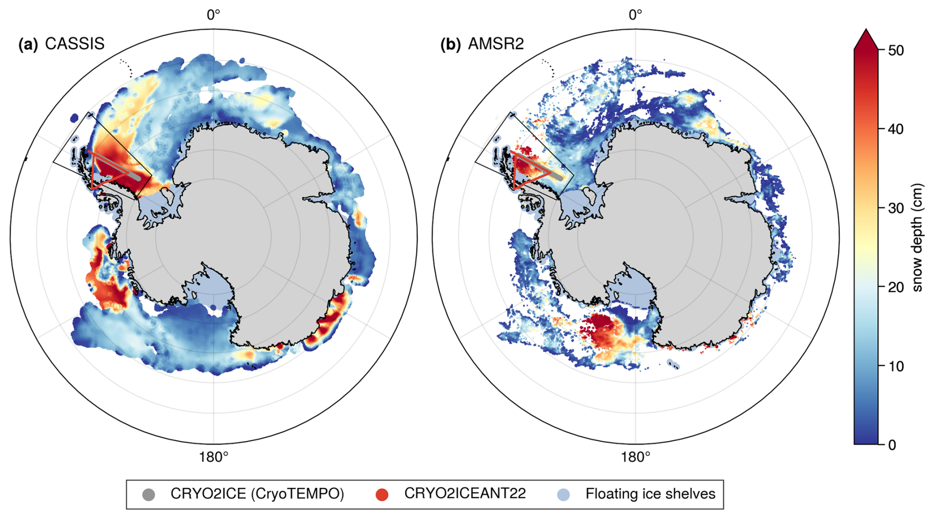
Figure 3 Pan-Antarctic snow depth distribution of 13 December 2022 from (a) CASSIS and (b) AMSR2. The location of the airborne CRYO2ICEANT22 track and collocated CRYO2ICE track is shown, and the black outlined box refers to the area showcased in Fig. 1 of Part 1. Floating ice shelves are provided in the NSIDC-0780 Antarctic regional mask data product (Meier and Stewart, 2023) at 6.25 km (using the NASA classification).

In addition, one may also question the freeboards obtained by CryoTEMPO, whether these are representative of the ice conditions within one CryoSat-2 footprint, or whether the ice conditions are too heterogeneous to derive a meaningful freeboard. While contributions of such ice conditions may not be distinguished in the CryoSat-2 waveforms due to the range resolution (∼ 0.47 m), a more restrictive classification scheme could remove such waveforms if confidence in the estimated freeboards is low and if they are considered ambiguous. Additional work is needed to identify if such a classification scheme is necessary for the CryoTEMPO product. However, the recent study by Müller et al. (2023) has shown the possibility of separating waveforms over thin ice from the ambiguous class, and providing freeboards over such ice would improve the ice conditions represented by the CryoSat-2 observations without favouring thicker ice. Currently, CryoTEMPO employs the physical retracker SAMOSA+, which is able to fit the waveforms, extract the tracking point based on assumptions of the distribution of surface scatters, and classify the waveforms independent of a restrictive classification scheme.

4.3 Comparison against airborne data

For the final comparison between the derived CRYO2ICE snow depths and the airborne snow depths derived along the under-flight, we compare the following snow depth combinations: ALS-Ku_TFMRA50, ALS-Ka_TFMRA50, ALS-Ku_MAX, ALS-Ka_MAX, ALS-${\mathrm{C}/\mathrm{S}}_{\text{MAX}}$, CWT, and PEAK, as these combinations are based on conventional assumptions. They are compared using airborne observations identified as sea ice floes (identified using the surface classification with pulse peakiness) and with snow depths above −0.05 m to limit the impact of viewing geometry accounting for measurement uncertainties. Furthermore, we also limit the upper threshold of snow depths to 1.5 m, assuming that higher snow depths are artefacts of the waveforms or viewing geometry or caused by limitations of the retrieval method (see Table 1 for data size constraints).

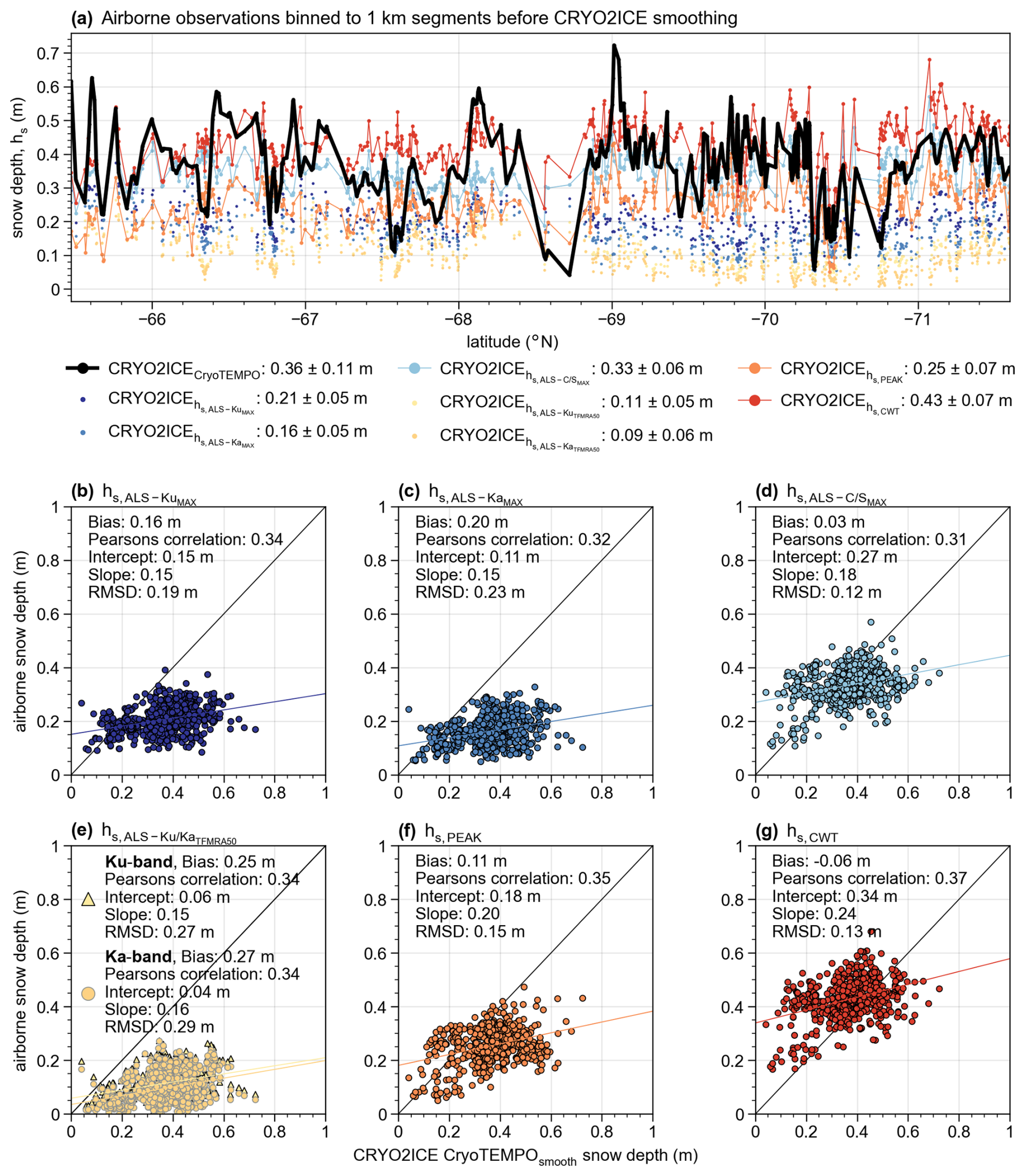
Figure 4 Comparison between airborne snow depth estimates and CRYO2ICE CryoTEMPO snow depths. Statistics computed for N=576 (coincidence of CRYO2ICE CryoTEMPO and airborne data). Bias computed as CRYO2ICE_CryoTEMPO–airborne snow depth. (a) Along-track comparison where airborne snow depths with most similar statistics are shown with both a marker and line. (b–g) Comparison between CRYO2ICE CryoTEMPO and each airborne product.

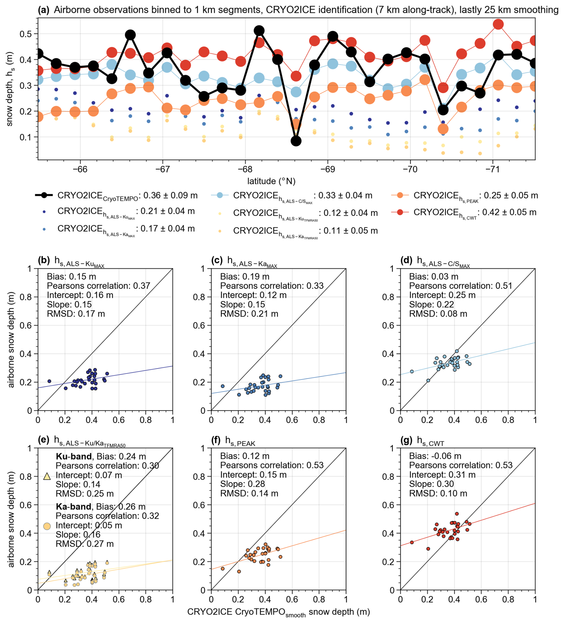
Figure 5 Same as Fig. 4 but with 25 km binning applied after CRYO2ICE identification. Statistics computed for N=28.

Table 1 Percentage of snow depth (h_s) observations identified as floes, at not a number (NaN), above 1.5 m, or below −0.05 m for the different combinations of airborne snow depth retrievals used in the comparison against satellite observations.

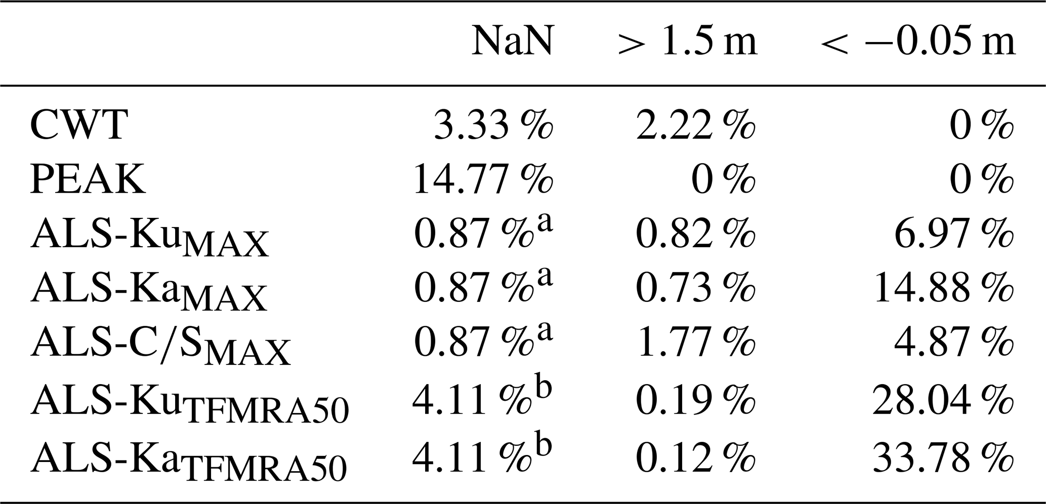
^a Since maximum power of waveforms is always available, this percentage denotes the times when there was not any ALS observations available within 5 m search radius of the radar to derive an along-track surface profile. ^b This percentage is a mix of the times when ALS was unavailable, or when the TFMRA50 retracker failed due to not being able to compute a threshold based on the restrictions set in Part 1.

First, we evaluate the comparison between the airborne observations and the CRYO2ICE CryoTEMPO observations by smoothing to the CRYO2ICE resolution from 1 km binned airborne snow depths (Fig. 4). Here, the highest correlations are observed for PEAK and CWT (0.35 and 0.37, respectively), although all seven airborne snow depth combinations show similar low to moderate correlations (0.31–0.37). The lowest bias is observed when using ALS-$\mathrm{C}/\mathrm{S}$_MAX of 0.03 m and with the lowest root-mean-square deviation (RMSD) of 0.12 m, followed by CWT with a bias of −0.06 m and RMSD of 0.13 m. PEAK presents a bias of 0.11 m and RMSD of 0.15 m. The other four snow depth combinations show significantly larger biases (0.16–0.27 m) and higher RMSD (0.19–0.29 m). Here, the spatial variability and resolution of the surface elevations clearly have an impact, and the fact that the airborne and satellites are observing in different ways seems to play a significant role.

We further evaluate the airborne and CRYO2ICE observations binned to 25 km segments (Fig. 5). While the bias remains the same for CRYO2ICE CryoTEMPO compared with both CWT and ALS-$\mathrm{C}/\mathrm{S}$_MAX, the correlations have greatly increased to a moderate correlation of 0.51–0.53 for ALS-$\mathrm{C}/\mathrm{S}$_MAX and CWT, respectively. RMSD has also decreased to 0.08 and 0.1 m, respectively. PEAK has increased by 0.01 m in bias but shares the highest correlation with CWT at 0.53 and has a decreased RMSD of 0.14 m. The other airborne estimates still have a lower moderate correlation of the order of 0.3–0.37 (with Ku_MAX achieving the highest), and with larger RMSD (0.17–0.27 m) and high biases (0.15–0.26 m). Overall, using a combination of ALS and $\mathrm{C}/\mathrm{S}$_MAX achieves the best result, which further supports the conclusion that the snow radar retrackers have discrepancies that need additional investigation.

We note here that there has been no ice drift correction applied between CryoSat-2 and ICESat-2 (where the time difference was approximately 2 h and 40 min) or between the airborne observations and the CRYO2ICE track (where the under-flight started approximately 1 h and 10 min after ICESat-2 overpass and ended approximately 1 h and 30 min after the CryoSat-2 overpass; see Sect. 2.1). While the airborne estimates themselves do not require ice drift correction since they were acquired on the same platform, there is, of course, a potential for misalignment when comparing the airborne estimates along both CryoSat-2 and ICESat-2 if used individually or if combined with CRYO2ICE (where ideally the observations would also be drift-corrected). Such a correction would require high temporal and spatial resolution drift observations of the order of hours and less than 7 km, which currently is not provided through publicly available products to the best of our knowledge. Fredensborg Hansen et al. (2024a) evaluated sea ice drift from daily medium-resolution products across 1 year's worth of CRYO2ICE observations and noted that, on average, the modal drift was of the order of a few kilometres between orbits Arctic-wide; hence, they would be minimised when smoothing with a 7 km along-track filter. Kwok et al. (2017b) presented average monthly-estimated drifts in the Weddell Sea of less than 10 km d⁻¹ and hence hourly drifts of less than a kilometre. Thus, we assume such drifts to be minimised with the CRYO2ICE smoothing, and we expect a further reduction of any drift impact when considering the 25 km segments.

5 Discussion and outlook

Arguably the most important aspect is considering how to collocate the radar observations acquired from ground-based as well as airborne and spaceborne instruments over sea ice. Willatt et al. (2023) evaluated the ground-based Ka/Ku-band radar system over Arctic spring-time sea ice and found that in the horizontal–horizontal (HH) polarisations (which are the current polarisations used on most airborne and spaceborne instruments, only the AWI IceBird carries a quad-polarised system) the strongest scattering in the majority of cases came from the a-s interface at both frequencies. Studies on their results over Antarctic sea ice from the Weddell Sea campaign in March/April 2022 are, at the time of writing, still pending; however, one might ponder whether similar results would occur considering the more complex snowpack of Antarctic sea ice and expected scattering further up in the snowpack. Importantly, Willatt et al. (2023) also argues that while the strongest scattering came from the a-s interface at Ku-band, scattering also did occur at the s-i interface, which could be leveraged. For example, they propose a waveform shape technique that assumes the trailing edge of the waveform includes information about the scattering further in the snowpack, which we also applied to the airborne observations (not shown). Unfortunately, it did not yield comparable results to the snow radar or provide much physical meaning when applied to Ka-band and Ku-band for this campaign. The derived snow depths using the waveform shape technique were approximately the same for the Ka-band and Ku-band, and the centroid used to denote the s-i interface rarely coincided with strong peaks on the trailing edge or corresponding snow–ice interfaces identified in the $\mathrm{C}/\mathrm{S}$-band, which we hypothesise is due to the specifications and resolutions of the instruments and the snow conditions observed.

There are several examples along our track, where it appears that the strongest scattering occurs at the a-s interface (also in agreement with findings from e.g., Fons and Kurtz, 2019; Willatt et al., 2010, 2011) but that significant, distinguishable scattering occurs further down supposedly at the s-i interface within the same radar waveform, suggesting that both interfaces contribute to the waveform and that both interfaces could be traceable even at Ku-band. However, tracking such interfaces would require a new, novel retracker able to detect smaller peaks below the main scattering horizon. Applying PEAK, which is able to detect up to five separate peaks regardless of whether they originate from the leading or trailing edge of the waveform, with the default parameters showed that, for some cases, it was able to track an interface below MAX. Tweaking the PEAK thresholds would allow for smaller peaks, which could be the s-i interface, to be retrieved; however, further work is required to understand how to fully apply this and which threshold values to use. Nonetheless, these findings suggest that both interfaces could – under the right circumstances and tweaked correctly – be retrieved from airborne Ku-band (and potentially Ka-band) alone, a suggestion also supported by De Rijke-Thomas et al. (2023) over Arctic spring-time sea ice. Additional work is necessary to evaluate under which conditions this applies both geographically (Arctic/Antarctic along with region/basin-specific) and seasonally. Similarly to the airborne data (Part 1, Sect. 5), the snow conditions also matter to the satellite observations, and the retracked scattering horizons are directly related to the instrument specifications of the spaceborne altimeters, as with the airborne data. Hence, any snow conditions (saline snow, icy layers, snow grains, etc.) limiting penetration at airborne scales are also expected to be impactful on the satellite scales, although at different magnitudes, which one may assume when the footprints are larger and the resolution lower.

Furthermore, current methods used to validate satellite observations with airborne observations apply similar retracking procedures at both scales for consistency without fully considering the fact that they are of different resolution and viewing geometry and may hold different information. Recent studies have aimed to evaluate which processes may play a significant role at different scales, as well as to what extent. For example, De Rijke-Thomas et al. (2023) presented some of the processes that may present differently from ground-based, airborne, and spaceborne scales dubbed as quasi-specularity. Hendricks et al. (2010) also noted that the airborne laser and radar altimeters could be statistically biased by the presence of smaller patches of open water (i.e., leads) or heavy ice deformation zones, observations also made in our study where the preferential sampling of the altimeters (radar or lidar) impacts the surface observed at footprint scales (leads vs. broken floes). A more in-depth dedicated analysis of the airborne data is necessary, and linking different sensors of different viewing geometries (laser vs. radar) and different penetration and backscatter signatures (using multi-frequency radars) is urged as a critical focus point to understand the full extent of where satellite multi-frequency altimetry is applicable.

The findings of this study suggest that the scattering mechanisms dominating at the Ka-band and Ku-band differ (with the Ka-band being more sensitive to different scatter interactions within the snow), resulting in several cases where the Ka-band's MAX occurred further down in the snowpack than the Ku-band. Evaluation of whether that is caused by the difference in dominating scattering mechanisms alone (e.g., volume scattering increasing biquadrate with frequency following the improved Born approximation Mätzler, 1998) or different ice observed by the radars still needs further work. However, future work on modelling the radar waveforms and understanding the backscatter contributions from different interfaces at the various frequencies with either 1D models such as multi-layer backscattering models as presented in Tonboe et al. (2021) or the Snow Microwave Radiative Transfer (SMRT) model (e.g., Meloche et al., 2024) is highly encouraged, provided viewing geometry, roughness, and resolutions are thoroughly considered and, to the best of abilities, accounted for. Investigating further is critical for the upcoming CRISTAL mission, but it is also critical for understanding the impacts of slant-looking Ka-band radar altimetry when using NASA's recently launched interferometric Surface Water and Ocean Topography (SWOT) mission, as well as for consolidating radar altimetry time series when considering different operation modes (from low-resolution mode (LRM) and pseudo-LRM to FF-SAR, SAR, and interferometric SAR) which also impact the retrieved waveform and the derived range.

Considering different viewing geometries, one may also consider whether the current CRYO2ICE methodology is applicable to Antarctic sea ice. One limitation for in-depth comparison is the limited number of CryoSat-2 radar freeboard observations, where both ESA-E and FF-SAR only provided observations for diffuse, non-ambiguous surfaces. However, were observations available (e.g., CryoTEMPO), comparison between airborne-derived snow depth estimates and CRYO2ICE CryoTEMPO would show similar statistics as for an along-track comparison with a monthly snow depth composite (Garnier et al., 2021). Discrepancies between snow radar and CRYO2ICE snow depths (using CWT and PEAK) present a current challenge associated with evaluating airborne and spaceborne-derived geophysical variables. Using lidar and $\mathrm{C}/\mathrm{S}$_MAX showed the highest agreement amongst all snow depth estimates derived at the 25 km scale. Additional work is encouraged for the evaluation of the CRYO2ICE orbits across the full Antarctic season to evaluate the information retrievable from near-coincident spaceborne laser and radar altimetry. This is especially relevant in preparation for CRISTAL, where understanding how to align observations – acquired even on the same platform (even if not at the frequencies expected for CRISTAL) – at different footprints and with potentially different scattering mechanisms should be approached. Here, the future airborne simulator for CRISTAL, known as CRISTALair (Garcia-Mondejar et al., 2023), will provide further insights and allow for continued dual- or even multi-frequency airborne observations to support research on consolidating different spatial scales.

For our study, we have not evaluated the relationship between roughness and the different retracked interfaces; however, it cannot be neglected and is therefore discussed here. Various roughness estimates and their relationships would need to be evaluated to understand how they impact the airborne radar observations, as well as how this is potentially translated into the spaceborne estimates. As such, one could compute a roughness estimate from the standard deviation of the lidar elevations within 5 m from the radar to evaluate the impact on the airborne observations further, similarly to De Rijke-Thomas et al. (2023). To provide a measure of roughness applicable towards the satellite scales, one must use the full swath. Here, roughness estimates could be computed per scan line following the methodology of Beckers et al. (2015) and Hutter et al. (2023), which could supply some information on the large-scale variability in roughness. Yet, such a roughness estimate only partially covers the CryoSat-2 footprint (400 m versus the cross-track Doppler-beam footprint of 1600 m) and provided at approximately every metre along-track (compared to the 300 m along-track footprint of CryoSat-2). Thus, significant work should be invested into understanding roughness at the different scales of the instruments, as well as how this may play a role. This is out of the scope of the current study but considered critical future work for the sea ice altimetry community. In addition, one must consider whether the roughness derived from the lidar (essentially, a measure of snow roughness) might be different from the sea ice roughness. Here, effects such as surfaces occurring smoother whenever snow redistributes around the rougher ice surfaces or rougher when snow features like sastrugi are created by wind redistribution likely have an effect. How and to what extent roughness from different interfaces impacts the radar pulse are also questions for future work.

It is critical that we continue and enhance the collection of consistent, detailed observations from a variety of spatial scales (ground-based to different areal components); however, without a strategically planned field-based campaign emulating what is observed from air to space, the evaluation of such observations is limited. However, without in situ components, validation of the airborne systems from different locations (regionally as well as dependent on the hemisphere, and considering the seasonal impact) cannot be independently ensured. Hence, the evaluation of the satellite observations, when compared to airborne observations, can only discuss similarities but not whether they are independently able to obtain the variables we expect given their observational capabilities.

6 Conclusions

In this study, we compared airborne snow depth estimates along a CRYO2ICE (CryoSat-2 and ICESat-2) under-flight carried out over the Weddell Sea on 13 December 2022 during the CRYO2ICEANT22 campaign. The derived airborne snow depth estimates (Part 1, Fredensborg Hansen et al., 2025) were compared with snow depth estimates derived along the CRYO2ICE orbit. The CRYO2ICE snow depths were also compared with two other Antarctic snow depth estimates (CASSIS and AMSR2) for further evaluation.

Comparison between three different CryoSat-2 processing chains showed large discrepancies likely caused by the waveform classification scheme utilised, as well as the ability to retrack waveforms from mixed-to-specular surfaces. Due to ESA-E and FF-SAR primarily retracking diffuse waveforms, their average radar freeboards along the CRYO2ICE track, whenever observations were available, were around ∼ 0.30 m. All three products had about 30 % negative freeboards. Comparing the derived CRYO2ICE snow depths showed, on average, CASSIS having 0.12 m thicker snow and AMSR2 and CRYO2ICE agreeing within 0.01 m (using CryoTEMPO as reference). Evaluating additional CRYO2ICE orbit across the Antarctic sea ice cover would be valuable to understand how well the snow depth variability can be retrieved along orbits using the established CRYO2ICE methodology.

We argue that future work should evaluate how we bridge different spatial scales (ground, air, and space) with the modelling of radar backscatter, taking into consideration viewing geometry, frequency, and footprints. Through comparison with the airborne-derived snow depth estimates (using ALS, Ka-, Ku-, and $\mathrm{C}/\mathrm{S}$-band “snow radar” observations) and binned to 25 km average, correlations of 0.51–0.53 were achieved with bias down to 0.03 m and RMSD of 0.08 m. The snow radar retrieval algorithms showed discrepancies but still a better agreement than with the snow depth estimates using Ka-band and Ku-band (in any combination with ALS and different retrackers), suggesting that the different processing methods from air and space, considering the different footprints, need further work to be made comparable. We strongly urge the community to further evaluate collocated past ground-based, airborne, and/or spaceborne observations from which new insights can hopefully be identified. Finally, we note that without an in situ component, we cannot state with certainty whether our satellite missions are able to retrieve what we believe they are retrieving. The same goes for the airborne data. Here, it is critical that we bridge the scales with ground, aerial, and satellite observations – ideally simultaneously – while accounting for the differences in spatial scales by sampling in patterns emulating what the satellite/airborne systems would observe. While this approach is dependent on logistics, weather, and sea ice conditions and whether the ground-based in situ campaigns are successful, these data are nonetheless a necessity to fully understand the capabilities of our remotely sensed observations, and must stay on the agenda when planning validation efforts.