the Creative Commons Attribution 4.0 License.
the Creative Commons Attribution 4.0 License.
 | 02 Oct 2025
Multi-frequency altimetry snow depth estimates over heterogeneous snow-covered Antarctic summer sea ice – Part 1: C∕S-, Ku-, and Ka-band airborne observations
Renée Mie Fredensborg Hansen
Henriette Skourup
Eero Rinne
Arttu Jutila
Isobel R. Lawrence
Andrew Shepherd
Knut Vilhelm Høyland
Fernando Rodriguez-Morales
Sebastian Bjerregaaard Simonsen
Jeremy Wilkinson
Gaelle Veyssiere
Donghui Yi
René Forsberg
Taniâ Gil Duarte Casal
The recent alignment of CryoSat-2 to maximise orbital coincidence with the Ice, Cloud, and land Elevation Satellite-2 (ICESat-2) over the Southern Ocean and Antarctica in July 2022, known as the CryoSat-2 and ICESat-2 (CRYO2ICE) Resonance Campaign, provided an opportunity to validate these satellites over land and sea ice. This was achieved through a simultaneous airborne campaign which involved an under-flight for near-coincident CryoSat-2 and ICESat-2 orbits in December 2022 and carried, amongst other instrumentation, Ka-, Ku-, -band radars as well as a scanning near-infrared lidar. This campaign resulted in the first multi-frequency radar evaluation of snow penetration over sea ice along near-coincident orbits. The airborne observations (at footprints of 5 m) revealed limited penetration of the snowpack at both Ka-band and Ku-band, with the primary scattering occurring either at the air–snow interface or inside the snowpack for both frequencies. On average, the Ka- and Ku-band scattering interfaces were 0.2 to 0.3 m above that for -band's primary scatter, where the average snow depth using -band reached around 0.5 ± 0.05 m depending on retrackers and combinations used. Interestingly, when the primary peak in the received signal occurs within the snowpack or at the air–snow interface, some scatter contributions are still present from the sea–ice interface at the Ku-band. This suggests a potential for snow depth to be derived from Ku-band signals alone by co-identifying these respective peaks in the waveform. Furthermore, it contradicts the assumption of a single scattering interface primarily contributing to the backscatter for Ku-band (and, to some extent, Ka-band) at airborne scales. The validity of this assumption needs further evaluation using former campaigns covering different sea ice conditions and seasons. With the unique combination of sensors and methods evaluated here, a shortcoming is the limited validation that can take place without strategically placed coincident in situ efforts. We call for coincident field initiatives as part of future validation campaigns considering the observational capabilities of airborne and spaceborne sensors when deciding on appropriate sampling strategies.
- Article
(7518 KB) - Full-text XML
- Companion paper
- BibTeX
- EndNote


Snow on sea ice plays a crucial role in the climate system of the polar regions with its insulating properties and high albedo, regulating sea ice growth and melt (Webster et al., 2018; Sturm et al., 2002). Beyond climatic importance and influence on the sea-ice–albedo feedback, snow depth plays a key role in the retrieval of sea ice thickness from satellite altimetry, as snow loading must be accounted for when assuming hydrostatic equilibrium. Hence, accurate and timely large-scale estimates of snow depth on sea ice are crucial. In particular, with relatively warm air temperatures even during freeze-up, strong winds, and heavy precipitation, the Antarctic sea ice is covered by an exceptionally heterogeneous snow cover (Massom et al., 2001). These conditions result in a wide variety of snow metamorphism occurring, complicating signatures observed using remote sensing methods. In particular, warm temperatures and variable atmospheric conditions can lead to, for example, large snow grain sizes and internal ice layers or ensure the presence of liquid water within the snowpack (Webster et al., 2018). Such conditions strongly interfere with the electromagnetic radiation from satellite observations. Coupled with a predominantly seasonal and relatively thin ice cover (Worby et al., 2008), the ice floes tend to depress below the water level due to the excessive loading of the snowpack, giving rise to snow-ice formation once flooded (Arndt et al., 2024). Finally, percolation of meltwater to the snow–ice interface during the austral summer can initiate the formation of superimposed ice (Arndt et al., 2021). Combined with the absence of strong surface melt, these conditions permit the survival of a year-round, highly complex, and diversified snow cover (Arndt and Paul, 2018).
Snow depth has been derived from altimeters by using a measure of the air–snow (a-s) interface and the snow–ice (s-i) interface (Kwok and Maksym, 2014), either from coincident surface elevations, range estimates, or freeboards (height of ice or ice + snow relative to the water level, depending on the frequency of the altimeter). Commonly, the a-s interface is identified using laser observations that reflect at (or very close to) the snow surface (Kacimi and Kwok, 2022, 2020), where the freeboard observations computed from lasers are referred to as the total freeboard (snow + ice). Ka-band altimeters are also usually assumed to have negligible penetration into the snow cover and are therefore often used as an estimate of a-s interface as well. Estimating the s-i interface has commonly been achieved by using Ku-band radars, where laboratory experiments have shown that Ku-band signals can penetrate to the s-i interface under cold and dry conditions (Beaven et al., 1995). Based on these experiments, Ku-band signals are often assumed to penetrate the snow cover, providing radar freeboards which are directly converted to sea ice freeboard after accounting for the slower wave propagation speed (e.g., Hendricks, 2022; Mallett et al., 2020). Several studies (e.g., Nab et al., 2023; Willatt et al., 2023, 2010, 2011; De Rijke-Thomas et al., 2023; Armitage and Ridout, 2015; Rösel et al., 2021; King et al., 2018; Nandan et al., 2017, 2020, 2023) have disputed this assumption based on comparisons using ground-based, airborne, and spaceborne observations, arguing that various interactions between the atmosphere, ice, and snow, such as snow metamorphism, redistribution, brine wicking, or flooding, can significantly limit the penetration of Ku-band waves. Nonetheless, this dual-frequency approach remains one of the few Earth observation methods to derive snow depth over sea ice, and it is currently one of the driving factors and main objectives of the future dual-frequency polar radar altimetry mission Copernicus Polar Ice and Snow Topography Altimeter (CRISTAL), planned for launch in 2027/2028 (Kern et al., 2020). For further investigation of the dual-frequency approach, ESA changed the orbit of their polar Ku-band radar altimetry mission, CryoSat-2, in July 2020 to align periodically with NASA's polar laser altimetry mission, the Ice, Cloud, and land Elevation Satellite-2 (ICESat-2) for the Northern Hemisphere. This alignment, known as the CRYO2ICE Resonance Campaign, was adjusted again in July 2022 to maximise orbits in the Southern Hemisphere. So far, near-coincident laser and radar observations have been collected over both hemispheres during the past 4 years with orbit maximisation efforts enabling the evaluation of snow depth estimates along-track across both hemispheres for at least 2 consecutive years (Fredensborg Hansen et al., 2024b).
To the best of our knowledge, no studies have fully evaluated the application of airborne multi-frequency altimetry for snow depth retrieval using lidar, Ka-band, Ku-band, and snow radars (with different ranges of frequencies having been flown but commonly covering -band and, more recently, also Ku-band) simultaneously in either the Arctic or the Antarctic since there, until now, has not been a campaign employing the full suite of instruments available. Most airborne studies have so far focused on (a) the Arctic snow depth using snow radars or combinations of snow radar and lidar (e.g.,Kurtz and Farrell, 2011; Newman et al., 2014; Rösel et al., 2021); (b) Ku-band radars combined with either ground-based reference observations or airborne lidars (e.g., Willatt et al., 2011; De Rijke-Thomas et al., 2023; King et al., 2018); or (c) deriving snow depth from snow radar, Ka-band, and/or Ku-band for the purpose of validating satellite observations (e.g., Garnier et al., 2021; Armitage and Ridout, 2015). Furthermore, while a variety of snow radar retrieval algorithms are available for Arctic applications (see, for example, Kwok et al., 2017, for an inter-comparison of snow radar retrieval algorithms applied to spring conditions), only a few studies have computed airborne snow depth and evaluated their applicability over Antarctic sea ice cover (e.g., Fons and Kurtz, 2019; Kwok and Kacimi, 2018; Kwok and Maksym, 2014; Galin et al., 2012; Panzer et al., 2013). Here, Fons and Kurtz (2019) presented some of the first airborne Ku-band results, showing that the main scattering horizon occurs closer to or at the a-s interface, indicating that the Ku-band scattering is also affected by the a-s interface.
Most observations acquired with either microwave snow radar sounders, -band radars, or lidars from airborne survey campaigns have been conducted through NASA's Operation IceBridge (OIB, 2009–2019), ESA's CryoSat Validation Experiment (CryoVEx, 2001–onwards), or Alfred Wegener Institute's (AWI) IceBird (2009–onwards). For sea ice, studies using NASA OIB have primarily relied on observations from a combination of lidar, snow radar, and optical sensors, which limits the potential for studies on Ka- and Ku-band signal penetration. 2009, 2010, 2011, and 2012–2016 campaigns carried several versions of a dedicated Ku-band radar at different frequency ranges (MacGregor et al., 2021). However, few studies utilise these data; for example, De Rijke-Thomas et al. (2023) used the 2016 Arctic campaign over landfast ice for dedicated analysis of airborne data, and Landy et al. (2021) used the 2011, 2012, and 2014 campaigns for evaluation of estimated sea surface height anomalies and radar freeboards using an optimised decorrelation framework. During the Arctic 2015 spring campaign, a Ka-band radar demonstrator was flown (MacGregor et al., 2021); however, to our knowledge, these data have not been further evaluated over sea ice. Lastly, campaigns after 2017 carried a combined 2–18 GHz snow radar (MacGregor et al., 2021; Rodriguez-Morales et al., 2020), which also covers the Ku-band frequency range, but sub-banding to evaluate the data at their specific bands at a cost of range resolution has not been fully explored. By analysing the radar returns over discrete sub-bands, Yan et al. (2017) demonstrated that the snow–ice interface appeared stronger over the 2–8 GHz sub-band versus the 12–18 GHz band, albeit at the expense of a degradation in vertical resolution with respect to the full 2–18 GHz. A difference at the air–snow interface was observed due to different surface roughness impacting differently depending on frequency. Furthermore, the above study noted that the interfaces were ambiguous for snow depths of less than 0.1 m, a direct effect of the degraded range resolution.
CryoVEx originally acquired Ku-band and airborne laser scanner observations over both Arctic and Antarctic land and sea ice to validate CryoSat-2, using the CryoSat-2 airborne simulator Airborne SAR Interferometric Radar System (ASIRAS), where SAR represents synthetic aperture radar. Based on the results of using SARAL/AltiKa (French–Indian Ka-band spaceborne pulse-limited radar altimeter in orbit since 2014) in combination with CryoSat-2 for snow depth retrieval (Guerreiro et al., 2016; Armitage and Ridout, 2015), efforts were made to include an airborne Ka-band sensor on the campaigns. Since spring 2017, CryoVEx has carried combinations of Ka-band and Ku-band sensors, originally as separate instruments, with ASIRAS and KAREN, and later through the combined Center for Remote Sensing and Integrated Systems (CReSIS) -band radar (flown on the CryoVEx 2019 summer and Cryo2IceEx 2022 spring campaigns, where both radars provide separate observations at their dedicated frequency bands). This instrumentation palette provides observations from lidars, Ka-band, and Ku-band along the same orbit, the only campaigns to fully employ and provide Ka-band airborne observations, from which both Ka- and Ku-band penetration can be further evaluated. Finally, CryoVEx in collaboration with the Natural Environment Research Council (NERC) Drivers and Effects of Fluctuations in sea Ice in the ANTarctic (DEFIANT) project completed an airborne campaign over Antarctic land and sea ice in December 2022 which under-flew a CRYO2ICE orbit (Fig. 1), a campaign that for the first time carried the full instrument suite including a snow radar, Ka- and Ku-band radars, and a scanning infrared lidar.
The AWI IceBird campaigns have been flying routinely in the Arctic since 2009, currently aiming for campaigns twice a year, i.e., during the Arctic sea-ice winter maximum in April and the summer minimum in August (Jutila et al., 2022a). The payload includes an airborne electromagnetic induction sounding sensor for total (snow + ice) thickness observations, along with a lidar and a CReSIS snow radar (2–18 GHz, since 2017) to derive the total freeboard and the snow depth, respectively. Currently, a method to derive snow depth from this particular snow radar has been developed; however, it has only been tested for the Arctic (Jutila et al., 2022b). One Antarctic campaign with a sea ice component has been conducted, but further analysis of the applicability of the methodology is pending.
With this two-part study, we bridge several gaps. In Part 1, we evaluate microwave penetration into Antarctic snow cover at Ka-band and Ku-band and the applicability of a -band snow radar, with comparison to lidar airborne observations. Here, we present the first in-depth evaluation of airborne coincident Ka-band, Ku-band, snow radar (-band), and lidar observations over sea ice. We note that the study is limited by the logistical challenges of airborne campaigns, and as such, the observations were acquired during the early Antarctic summer season. Hence, the physical conditions of the snow and ice pack on Antarctic sea ice likely limit the full evaluation of the various retrieval algorithms and data available for all surface, sea ice, and snow conditions. From the evaluation of the airborne data, we then compare airborne snow depth estimates derived from traditional hypotheses of penetration with near-coincident spaceborne radar (CryoSat-2) and laser (ICESat-2) orbits along a dedicated CRYO2ICE orbit, which is currently the only CRYO2ICE validation under-flight carried out with a full suite of instruments able to evaluate penetration into snow. This is presented in Part 2 (Fredensborg Hansen et al., 2025) (hereafter cited as Part 2).
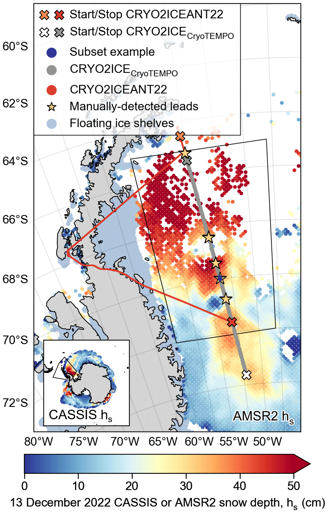
Figure 1Cryo2IceEx and NERC DEFIANT 2022 (CRYO2ICEANT22) campaign with under-flight on 13 December 2022 along the CryoSat-2 and ICESat-2 (CRYO2ICE) orbit with the location of subset example used throughout the study and location of manually detected leads for offset calibration overlaid with the AMSR2 snow depth product (for the main figure) and the CASSIS (Centre for Polar Observation and Modelling (CPOM) Antarctic Snow on Sea Ice Simulation) product (for inset); see the “Data availability” section for references to data products (which are further utilised in Part 2). Note that the CryoTEMPO product refers to a specific processing chain used for CryoSat-2 observations, which are further evaluated in Part 2. The black outline in the inset denotes the map extent shown as the main figure; black outline in the main figure denotes the area of interest for ERA5 precipitation and temperature calculations (see also Fig. 2). Floating ice shelves are provided in the NSIDC-0780 Antarctic regional mask data product (Meier and Stewart, 2023) at 6.25 km (using the NASA classification).
Table 1Radar parameters. If only one value per parameter is provided per row, the same value stands for all radars. Values in parenthesis denote average and standard deviation.
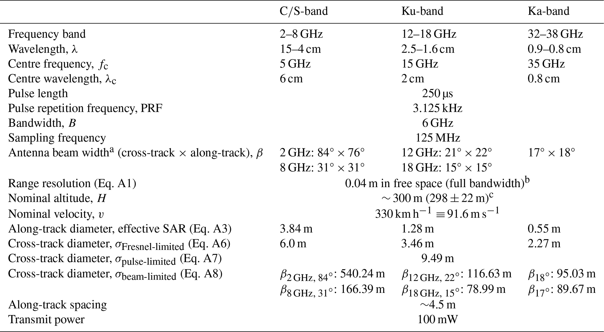
a Manufacturer of Ka-band antennae does not provide a number versus frequency, only for the full range. b Often, processing is completed for a smaller bandwidth, resulting in a slightly coarser resolution. c Based on the elevation variable in the CReSIS data profile.
2.1 Cryo2IceEx/NERC DEFIANT 2022 (CRYO2ICEANT22) airborne campaign
ESA continued their validation programme CryoVEx in collaboration with the Technical University of Denmark (DTU) National Space Institute (DTU Space), CReSIS, University of Leeds, and the British Antarctic Survey (BAS) under the ESA Cryo2IceEx and NERC DEFIANT projects in December 2022 (29 November to 20 December). The 2022 airborne campaign (dubbed CRYO2ICEANT22) focused on the validation of multi-frequency altimetry observations along coordinated CryoSat-2 and ICESat-2 orbits over both land and sea ice, including the dedicated CRYO2ICE orbit over sea ice in the Weddell Sea. The survey flights were carried out using a BAS DASH-7 aircraft from Rothera Research Station. The instrument package included Ka-, Ku-, and -band radar altimeters from CReSIS; an airborne laser scanner (ALS) of the type Riegl LMS Q‐240i‐80; five dual-frequency GNSS Javad Delta receivers; a high-precision inertial navigation system (INS) of the type iMAR (Jensen, 2024); four GoPro 9/10 cameras; an Eppley radiometer with pyranometer and infrared thermometer; and GNSS-R (reflectometry). For this study, we focus only on the radar and lidar observations that have been pre-processed using data from the GNSS receivers and iMAR INS as input. We only utilise visible imagery from the nadir-looking GoPro as qualitative validation of our surface classification.
During the campaign, there was no in situ component for local observations of snow depth or ice conditions on sea ice, nor were there other reference observations available to provide input on the conditions (e.g., active AWI snow depth and ice mass balance buoys during December 2022 (ID 2017S54, 2022S110, 2022T88) did not drift far enough from the Neumayer III research station to be covered by the orbit; see Grosfeld et al., 2016). Thus, we have to rely on ERA5 reanalysis estimates (see Fig. 2, Sects. 2.2 and 5) of precipitation and air temperature for the discussion on radar penetration and the impact on snow conditions.
2.1.1 radar and snow radar
The CReSIS Ka- (32–38 GHz), Ku- (12–18 GHz), and -band (2–8 GHz) radars were provided by the University of Kansas, and they allow for resolving various layers (e.g., snow versus ice over sea ice) depending on surface conditions (Rodriguez-Morales et al., 2014). The radars operate in frequency-modulated continuous-wave (FMCW) mode over a wide bandwidth, resulting in a fine (a few centimetres) vertical resolution depending on the bandwidth. Depending on the surface conditions, -band has a vertical resolution of 0.02–0.04 m (in snow), whereas Ku-band and Ka-band have a vertical resolution of approximately 0.04 m (Rodríguez-Morales et al., 2021; Panzer et al., 2013). For the campaign, the radars can be accommodated in different modes, where the default mode is full bandwidth, which supports simultaneous acquisition of all three radars in their full frequency range at altitudes up to ∼ 1200 ft (∼ 365 m) above ground level (a.g.l.), with an optimal operating altitude at 1000 ft (300 m) and a minimum altitude of 800 ft (240 m). At nominal flight altitudes, the diameter of the footprint of the radars is of the order of 5 m. For a detailed description of the pre-processing steps resulting in the radar waveforms used in the study, see Appendix A.
During the under-flight, the radars were turned on (off) before (after) reaching the intended CRYO2ICE orbit ground track to ensure that the instruments were running as expected when at the location. During these stretches, as well as during calibration manoeuvres, the radars are likely to experience signal degradation due to various flight manoeuvres (e.g., turns, too high altitude), which should be filtered out from the science data. Due to the segmentation of the CReSIS data into frames and the activation of truncation procedures (see Appendix A3), the size of the waveform parameter changes significantly during such manoeuvres (the number of range bins increasing from approximately 1200 to 25 000 or even more). For processing a full flight and combining all frames into one file, we consider only the frames where the aircraft was aligned with the intended satellite orbit (frames 74–232 selected manually; see extent in Fig. 1) and within the altitude of the default mode, resulting in range bin sizes of the order of ∼ 1200 and an along-track distance coverage of 792 km.
2.1.2 Airborne laser scanner (ALS)
The Riegl LMS Q-240i-80 ALS, provided by the BAS, uses three rotating mirrors, resulting in parallel scan lines on the surface with a maximum scan angle of 80°. It operates in the near-infrared (NIR) with a wavelength of 904 nm, assumed to reflect at the a-s interface. While NIR (904 nm) waves are generally assumed to reflect from first-encountered surfaces, they are likely to penetrate several centimetres under optimal cold, low-density surface snow (Deems et al., 2013). However, we assume that under these conditions such a potential penetration is negligible. The ALS has a pulse repetition frequency of 10 kHz and a sampling configuration of 40 scan lines per second with 251 shots per line, providing regular coverage of the surface at nominal flight speeds. This configuration provides 1 observation per square metre with an illuminated footprint of close to 0.7 m in diameter at a nominal flight height of 300 m a.g.l. and ground speeds of 250 km h−1. This corresponds to a cross-track swath width of approximately 400 m, and a laser shot-to-shot accuracy of a few centimetres. The ALS point clouds were combined with GNSS-INS solutions using precise point positioning (PPP) to provide ellipsoidal heights. Ellipsoidal heights are elevations relative to the reference ellipsoid, in this case World Geodetic System 1984 (WGS84). This is computed as the range obtained from retrackers (Sect. 3.1) subtracted from the altitude of the aircraft or spacecraft. Precise orbit and clock information, provided routinely by the International GNSS Service (IGS), was used. This allows for accurate solutions even for flights with long baselines. Offset angles between ALS and INS measurements were calculated and applied using standard calibration procedures (Skourup et al., 2024, currently under final review at ESA as of September 2025).
2.1.3 Visual cameras
The DASH-7 was equipped with a nadir-looking GoPro 10 with an image size of 5568×4176 pixels and a resolution of 72 dpi. The GoPro uses an internal GNSS mode and is set to capture images at 0.5 s intervals, with a field-of-view corresponding to approximately the ALS swath width. This setup ensures along-track overlapping images. The calibration procedures of the cameras are similar to those for the ALS.
2.2 ERA5 2 m air temperature and precipitation
Ideally, for the validation of snow depth derived from airborne -band combinations, in situ observations would be collected to provide a ground truth to compare against. However, during this campaign, there was no in situ sea ice component. Instead, we utilise estimates of precipitation and temperature from the ERA5 reanalysis data set within approximately ±1 month of the under-flight date to evaluate the potential impact of atmospheric events. ERA5 provides estimates of several atmospheric, land, and oceanic climate variables (Hersbach et al., 2023). Here, we utilise the 2 m air temperature, total precipitation, and snowfall parameters, all available on a regular 0.25° × 0.25° grid, averaged to daily resolution from 1 November 2022 to 31 December 2022. We use these observations to evaluate the temperature and precipitation conditions before, during, and after the campaign by computing the minimum, maximum, and average values of each parameter within a bounding box around the airborne flight path covering sea ice (see Fig. 2).
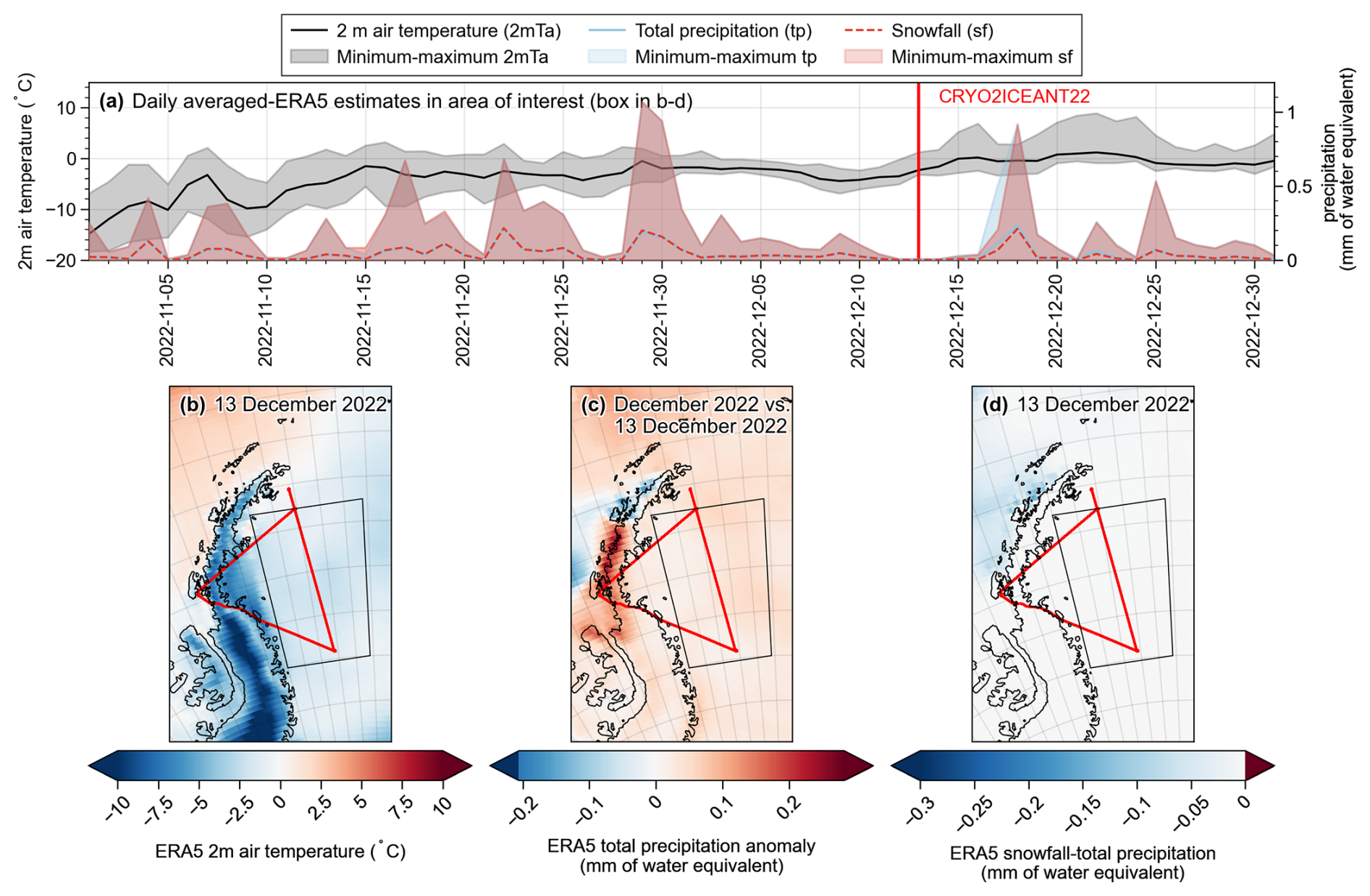
Figure 2(a) ERA5 daily averaged 2 m air temperature and precipitation (total precipitation and snowfall) for 1 November to 31 December 2022, computed for the area marked by the black outline in (b)–(d). (b) 2 m air temperature on 13 December 2022, (c) total precipitation anomalies, computed as the difference on 13 December compared to the December 2022 average, and (d) the difference between snowfall and total precipitation on 13 December 2022. The CRYO2ICEANT22 under-flight on 13 December 2022 is outlined in red (b–d and Fig. 1).
3.1 Surface retrieval methodology (retrackers) for airborne radar altimeters
To extract the surface elevation from radar altimeters, one must identify the precise point on the radar echo (power spectrum, i.e., the waveform) that corresponds to the surface being measured (the retracking point) using a retracker. Various retrackers are used in altimetry, and based on the measurement technique (snow radar or -band radars), one may either apply a retracker to extract a single surface scattering horizon as the dominant interface or multiple scattering horizons based on the assumption that the radar echo contains information about several interfaces. The multiple-interface approach is the main assumption applied to observations from FMCW snow radars, where the goal is to retrack the a-s and s-i interfaces. In contrast, for conventional altimeters, such as Ku- and Ka-band radars, the aim is to retrack the surface from which most backscatter is reflected, assuming one interface dominates the signal. Here, we specify the retrackers used in this study for the extraction of single and multiple scattering horizons.
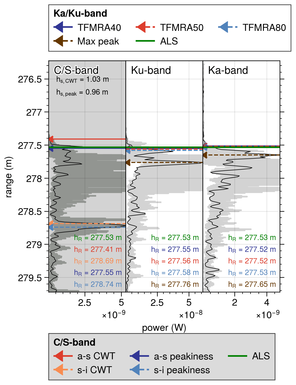
Figure 3Individual waveform examples (in black) for each radar (Ku-band, Ka-band, or -band) are provided, including the location of retracking points using various retrackers (depending on the radar). The corrected range at different retracking horizons (hR) and derived snow depths (hs) for multiple scattering horizons using different retrackers are also presented. In addition, the ±5 closest neighbouring waveforms (in grey) are shown to illustrate local variations in the waveforms. Here, Ka-band and -band have been aligned with the Ku-band's z axis (using the lever arms provided in Appendix B) with m and m, where z denotes the downward direction from the aircraft (or the range).
3.1.1 Single scattering horizons
The threshold first-maximum retracker algorithm (TFMRA) is commonly used for satellite radar altimetry observations acquired over sea ice, where studies have investigated and currently apply different retracking thresholds (40 %, 50 %, 70 %, or 80 %; see, for example, Ricker et al., 2014; Tilling et al., 2018; Lawrence et al., 2018; Garnier et al., 2021; Hendricks, 2022). For TFMRA, we retrack only points above the thermal noise level, determined as the average of the first 50 bins of the waveform. Three retracking thresholds are applied (40 %, 50 %, and 80 %) to the first maximum. The first maximum is identified using a 30 % threshold of the maximum value, and the retracking threshold is then applied to the first maximum to derive the range to the surface and, ultimately, the elevation. While the most commonly used empirical retrackers for spaceborne sea ice altimetry employ TFMRA at 50 % or 70 %, recent airborne studies have investigated using a threshold-maximum retracker algorithm at 70 % (De Rijke-Thomas et al., 2023). This algorithm uses the maximum power of the waveform to identify the surface, regardless of the origin of the backscatter. We also extract the maximum power here to evaluate the origin of the dominant scattering interface, although we do not use a threshold on the leading edge of the absolute maximum (similarly to ground-based studies of Willatt et al., 2023, where they also utilise the maximum amplitude, within a specific range window of expected surface scattering to reduce the impact of side lobes, as the main scattering interface).
3.1.2 Multiple scattering horizons
Currently, numerous retrieval methods for extracting a-s and s-i interfaces for snow radars exist, and several have been inter-compared over Arctic sea ice (Kwok et al., 2017). However, only two algorithms are currently provided as open-access software; hence, we only process the snow radar with those retrackers.
Newman et al. (2014) presented the continuous wavelet transform (CWT) retracker for the detection of snow and ice interfaces from the CReSIS snow radar systems. This retracker is capable of identifying interfaces independent of radar systems and without relying on specified thresholds. Instead, CWT aims to detect two interfaces on the leading edge of the waveform by first identifying the range bin where the power first rises above the noise floor on the leading edge of the waveform. This range bin is expected to represent the illumination of the first interface (a-s). To identify the s-i interface, the range bin on the leading edge exceeding a level of noise and an estimate of radar clutter is selected. This bin is expected to represent the illumination of an interface with the highest power reflection coefficient (the theoretical s-i interface). This is achieved by preconditioning the echogram to make these locations more distinguishable. Since the s-i interface, under relatively undeformed and cold conditions, shall contribute most to the power distribution, no modification of the echogram is applied for retracking. However, for detecting the a-s interface, the logarithm of the radar echogram is taken to make the theoretical location of the a-s interface more distinguishable. The discretised version of the CWT is applied to find the two interfaces by the use of Haar wavelets, which are scaled step functions designed primarily to find sudden transitions within signals. The coefficients of the wavelets are summed to detect an interface, identified as the value where the summed coefficients are maximised. Here, the benefit is that it is independent of a set of fixed thresholds and that it is not affected by changes in transmitted power and received noise, which vary depending on the radar system. Based on evaluation over first-year and multi-year Arctic sea ice, uncertainties were recorded at ∼ 0.06 m over low-topography targets (Newman et al., 2014).
Jutila et al. (2022b) developed the peakiness retracker (PEAK) specifically for the CReSIS 2–18 GHz snow radar system used on the AWI IceBird campaigns. This retracker enables snow depth retrievals even in more complex snowpacks, particularly in cases where the a-s interface is the main scattering surface. It is based on left- and right-handed pulse peakiness (PP) parameters following Ricker et al. (2014) as well as logarithmic and linear scale power thresholds. To detect the a-s interface, the normalised waveform is analysed using the logarithmic scale similar to Newman et al. (2014). The first peak that is above the noise level by a user-defined power threshold and satisfies a user-defined left-hand peakiness threshold is defined as the a-s interface. The s-i interface is located in a similar way but using the normalised linear scale waveform, linear scale power threshold, and right-hand peakiness threshold analysing up to five peaks. The last peak satisfying the thresholds is identified as the s-i interface, whether it is the maximum peak or not. If more than five peaks satisfy the thresholds, the waveform is regarded as ambiguous, and no interface locations are returned. The uncertainty of the retrieved snow depth was estimated to be 0.04 m (or 18 % of the snow depth) over level and landfast first-year sea ice. A detailed description can be found in Jutila et al. (2022b). A disadvantage of this method is its dependence on user-defined thresholds, which ideally should be verified with coincident ground-based measurements to ensure its accuracy.
Both retrackers are applied using the open-source Python package pySnowRadar (King et al., 2020), where for CWT the following default parameters are used: one reference snow layer and a CWT precision of 10. For PEAK, the following default parameters are used: a logarithmic peak threshold of 0.6, a linear peak threshold of 0.2, and both left and right peakiness thresholds of 20. An example of derived ranges using the retrackers presented herein on the airborne observations for all three radars is shown in Fig. 3. It is important to note that residual range side lobes, which have been reported as an issue in previous studies (Kwok and Haas, 2015; Kwok and Maksym, 2014), have been significantly reduced through the use of the current version of the CReSIS processing chain. Additional steps can be taken to remove snow depths over highly deformed ice (provided through a topography parameter) using coincident lidar observations; however, this has not been applied in our study due to inconsistencies between ALS and the a-s interfaces identified by the snow radars (see Sect. 4.1).
3.2 Pre-processing of airborne surface elevations and surface discrimination
Additional processing must be applied to the airborne observations (a) to derive a nadir lidar profile along the swath for comparison with the radar observations, (b) to align the lidar and radars by applying a calibration offset to account for internal delays in the radar system, and (c) to distinguish between floes and leads for comparing snow depth estimates only on floes.
3.2.1 Deriving nadir lidar profile along ALS swath
We extract a nadir lidar profile as the average of ALS observations within a search radius of 2.5 m from the centre location of each radar observation (latitude and longitude); see an example of the location of the nadir profile in Fig. 4a. This methodology has also been implemented in De Rijke-Thomas et al. (2023) and Jutila et al. (2022b). The nadir ALS profile allows for evaluation of where the radar scattering occurs within the snowpack along the flight track, assuming that the lidar scatters at the a-s interface. We note here that in the presence of broken floes or a highly heterogeneous ice cover (e.g., leads with small ice floes in between), the lidar will favour scattering from the ice floes as opposed to specular surfaces such as leads (which has also been discussed by Hendricks et al., 2010). Hence, in the case of such surfaces, the nadir lidar profile may reflect a different ice surface than the radar, as the radar instead will be dominated by specular returns from leads. This is further discussed in Sects. 4.3 and 5. Laser observations where the absolute difference of the radar elevations (derived using TFMRA50) and nadir laser profile are more than 3 m are noted as “not-a-number”.
3.2.2 Offset calibration to align radars with lidar
To account for internal delays in cables and electronics, a calibration offset (Δ) between the ALS and radars (with the radar observations subtracted from the lidar observations) must be computed to obtain aligned absolute surface heights. We compute this offset using manually identified specular surfaces, i.e., leads along the flight track, where the laser and radars are expected to reflect from the same surface. We manually identify seven leads (∼100 observations) and compute the mean offset per detected lead (see Table 2) from the ellipsoidal heights. From the seven mean offsets, we compute the mean offset per frequency band. It is important to note that within leads the TFMRAs at any given threshold provided the same offset, except for the Ka-band at 80 %, which was 0.02 m lower than the offsets at the other tested thresholds. For this study, we apply the calibration offsets of 0.34 and 0.22 m for Ku-band and Ka-band, respectively, neglecting the changes for Ka-band at 80 % which are within the range resolution of the altimeter. For -band, we used a-s and s-i interfaces identified with the PEAK retracker to compute the offsets, which resulted in 4.54 m for both interfaces. Using the CWT retracker, we obtained offsets of 4.74 and 4.58 m for the identified a-s and s-i interfaces, respectively. This indicates a bias compared with PEAK, leading to thicker snow estimates when using the CWT retracker. Specifically, CWT would retrack 0.04 m below the s-i interface compared with PEAK and 0.2 m above the a-s interface, assuming that the retrackers consistently retrack the same difference between interfaces. This results in a 0.24 m difference, equivalent to ∼0.19 m of snow depth, when using a snow density of 300 kg m−3. However, it is likely that the interfaces are retracked differently depending on the surface conditions and the resulting waveform shape; thus, the bias may vary depending on the waveform. We note that PEAK is used as a reference since it identified the same offset over leads for both interfaces. The calibration offset for the snow radar does not impact derived snow depths using PEAK or CWT, since these are based on relative measurements between the identified interfaces and are not calibrated to align with the ALS observations. We note that the alignment of the calibration is based on the assumption that the retracker successfully and correctly retracks the lead at the same elevation. However, due to the increased range resolution of the airborne radar, the different retrackers may select different range bins as the time when the surface is best illuminated. Thus, we also provide the offset to the maximum power in leads for each band. Here, the offset is computed as 0.31, 0.19, and 4.54 m for -band, Ku-band, and Ka-band, respectively, presenting biases of 0.03 m for both Ku-band and Ka-band using TFMRA50 as reference (although within the range resolution of the airborne system). There was zero bias for -band when referenced to PEAK a-s. This suggests that PEAK is successful in identifying the correct interface over leads, whereas CWT will retrack the a-s significantly before.
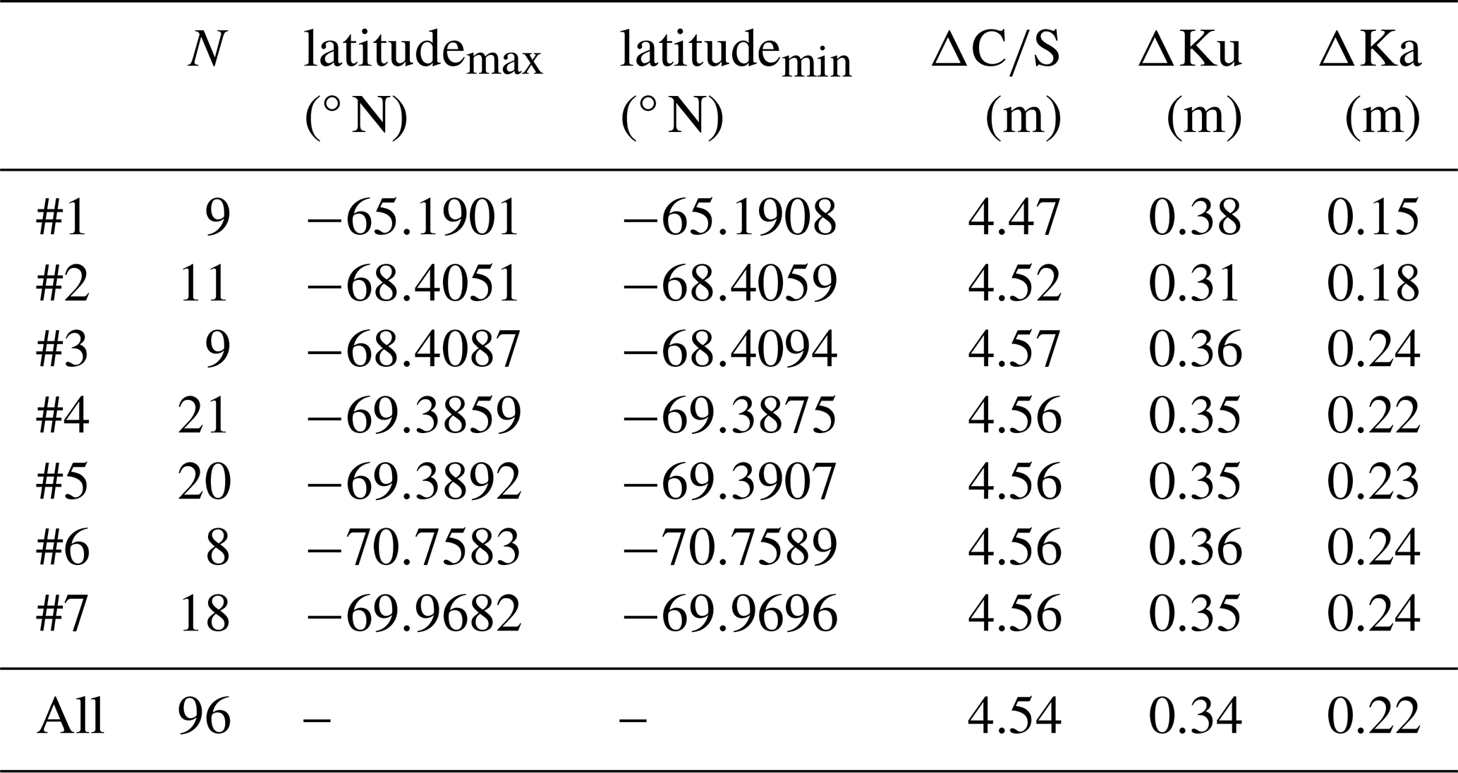
Table 2Manually detected leads from airborne observations used to compute the calibration offset (Δ) between ALS and the radar system for each frequency band. The last row includes the sum of all observations and the average offset of each frequency band. The offsets shown here were calculated with TFMRA50 for Ka-band and Ku-band, as well as the PEAK retracker at the a-s interface (discussed further in Sect. 3.2.2). N denotes the number of individual observations used per lead identified.
3.2.3 Discrimination between floes and leads in airborne radar observations
The necessity of discriminating observations from leads and floes is twofold. First, the radar and ALS observations perceive the surface differently, with specular reflections from the water dominating the radar signal. Simultaneously, small floes within the radar footprint might be present in the ALS swath and included in the observations used to generate the nadir laser profile. This results in an increase in the elevation over leads compared with the radar-derived elevation, which would provide a snow depth estimate when differencing laser and radar if not properly classified. Second, the aim of this study is to derive snow depth using multi-frequency altimetry; therefore, we are only interested in snow depth estimates over floes. To discriminate between floes and leads, it is common in spaceborne radar altimetry to use a multitude of waveform parameters such as maximum power (MAX) and PP, along with other waveform parameters specific to the delay-Doppler processing of SAR altimeters (e.g., Ricker et al., 2014; Tilling et al., 2018, applied to Arctic studies). MAX is defined as the highest power within the range window, and PP is computed as
where NWF denotes the number of range bins, PMAX is maximum power, and Pi is the power of the ith range bin. For easier visualisation, we convert to normalised values using maximum–minimum normalisation. Converting from normalised waveform parameters and back, we use , where y denotes the original waveform parameter value, yNORM denotes the normalised waveform parameter, and x is the array of the waveform parameter. We note that, while we use similar formulas to derive the waveform parameters as those used for spaceborne (and airborne, for example, Zygmuntowska et al., 2013) altimeter observations, we do not necessarily expect similar thresholds due to the different instruments and platforms. Instead, we derive specific thresholds discriminating between floes and leads in the CReSIS radar. For PP, we compute PP from −100 and +156 bins after MAX to align with the number of range bins for CryoSat-2 and to limit the impact of thermal noise on the estimated PP values.
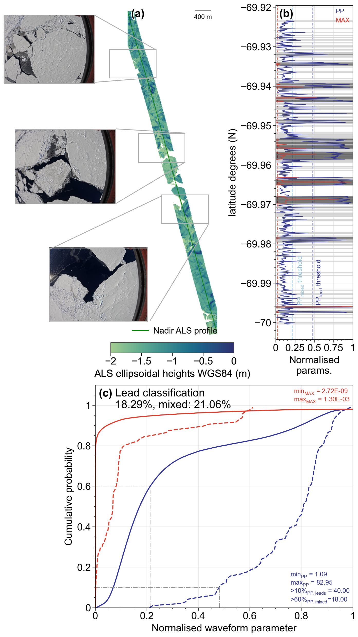
Figure 4Discrimination of sea ice floes and leads in the airborne observations. (a) ALS swath along with optical images to visually confirm the surface classification. (b) Normalised waveform parameters (pulse peakiness (PP) and maximum power (MAX)) shown along the nadir track of panel (a) with the identified surface types “leads” and “mixed” (based on panel c) highlighted as dark grey and light grey horizontal lines, respectively. The thresholds determined from panel (c) are also shown in panel (b) as dashed vertical lines. (c) Cumulative probability distribution of waveform parameters MAX (red) and PP (blue) for the entire flight (solid lines) and manually detected leads (dashed lines) are shown. Minimum and maximum values for the waveform parameters are provided, along with downwards rounded waveform parameter values at 10 % (“leads”) and 60 % (“mixed”), which are used to identify surfaces based on comparisons with the cumulative distributions of each surface type. The statistics of observations classified as “leads” and “mixed” surfaces are provided for the entire under-flight. Grey dashed lines align the chosen cumulative probability thresholds with the location of the respective distribution used.
We find that PP provides the strongest discrimination between surface types, shown by strong separation in the cumulative probability of the two distributions and minimal separation for MAX (Fig. 4c). From the cumulative distributions (Fig. 4c), we use the 10 % cumulative probability of PP, applied to the distribution of manually detected leads, as our lower bound for leads and 60 % cumulative probability for the distribution of the entire flight (approximately where the distribution of leads starts) as lower bound for mixed surfaces. Both values are rounded down to integers. Visual inspection of the waveform parameters and their lower bounds in Fig. 4b, compared with the ALS swath in Fig. 4a, supports the surface classification thresholds. Along the orbit, PP ranged between 1.09–82.95 with a 10 % lower bound threshold of 40 using the distribution of manually detected leads and a 60 % lower bound with PP of 18 using the full distribution, values which coincide well with the thresholds from former studies. Here, Ricker et al. (2014) classified leads through a combination of waveform parameters including PP ≥40, and Tilling et al. (2018) denoted specular surfaces as PP ≥18. In Tilling et al. (2018), mixed surface types had PP down to 9, from which one might argue that our classification is less robust and some mixed surfaces might still be included in the processing. Applying the requirement of leads and mixed surfaces having PP above thresholds of 40 and 18 (until 40), respectively, we identify 18.29 % of the observations as leads and 21.06 % as mixed (a total of almost 40 % of observations), and we remove these from further processing of snow depth estimates and evaluation of radar penetration.
3.3 Retrieval of snow depth from altimetry freeboards and/or elevations
Similar to Kwok et al. (2020), we calculate snow depth (hs) by differencing the height of interfaces at a-s (ha-s), equivalent to the total freeboard, and s-i (hs-i), equivalent to the sea ice freeboard, following
The sea ice freeboard (or s-i interface, hs-i) is related to the radar freeboard, assuming full penetration to the s-i interface, which is often considered the case for Ku- and C-band radars, as follows:
The second term in Eq. (3) accounts for the reduced propagation speed of the radar wave (cs) as it travels through the snowpack with a bulk density ρs assuming a cold and dry snowpack. The refractive index (ηs) at Ku-band is (Ulaby et al., 1986), and c is the speed of light in free space. Through combination of Eqs. (2) and (3), snow depth (hs) is given by
Now, snow depth (hs) is related to the differences between the a-s and s-i interfaces (extracted by a radar) with one free parameter, ηs, which is dependent on the snow bulk density and directly related to the snow conditions. Massom et al. (2001) presented an overview of Antarctic snow conditions from field observations acquired between 1992 and 1998 under a variety of seasonal and geographical conditions. The average snow density values from a number of studies ranged between 247 and 391 kg m−3, while the overall range was from 99 to 817 kg m−3. These results have guided some studies (e.g., Kwok and Kacimi, 2018; Kacimi and Kwok, 2020) to use 320 kg m−3 as their reference bulk snow density. Kwok and Maksym (2014) used 300 kg m−3 and noted that with a snow density uncertainty of 50 kg m−3 the overall uncertainty of radar-derived snow depth ranged between 0.03 and 0.05 m for snow depths between 0.1 and 0.7 m. One could argue for using a bulk snow density of ∼350–360 kg m−3 in this study, as the observations were acquired during Antarctic summer (December to February), and this value is used for that time period in the seasonal varying snow density scheme applied to CASSIS (Lawrence et al., 2024, their Fig. 2a). While Kacimi and Kwok (2020) noted that there is no accepted bulk density of Antarctic snow, Massom et al. (2001) suggested 200–300 kg m−3 under cold and dry conditions and a higher density (320–500 kg m−3) for warm and windy conditions. Here, we present a sensitivity study on the impact of choosing different bulk snow densities. Figure 5 shows that even for very thick snow depths, using either 300, 320, or 350 kg m−3, the maximum difference was m. Therefore, we do not expect a large impact when using slightly different snow densities, which is within the order of the resolution of the airborne instruments themselves. Instead, the largest differences occur under extreme events at the edges of the density range. For the densities reported by Massom et al. (2001), differences range from −0.13 to 0.08 m in these cases (using a range of 150–600 m−3). However, we note that in the case of extreme cases, the largest impact will likely be seen on the (in)availability of detected s-i interfaces rather than on the derived snow depth. Based on this sensitivity analysis and the limited impact of derived snow depth, we keep the bulk density of snow constant at 300 kg m−3.
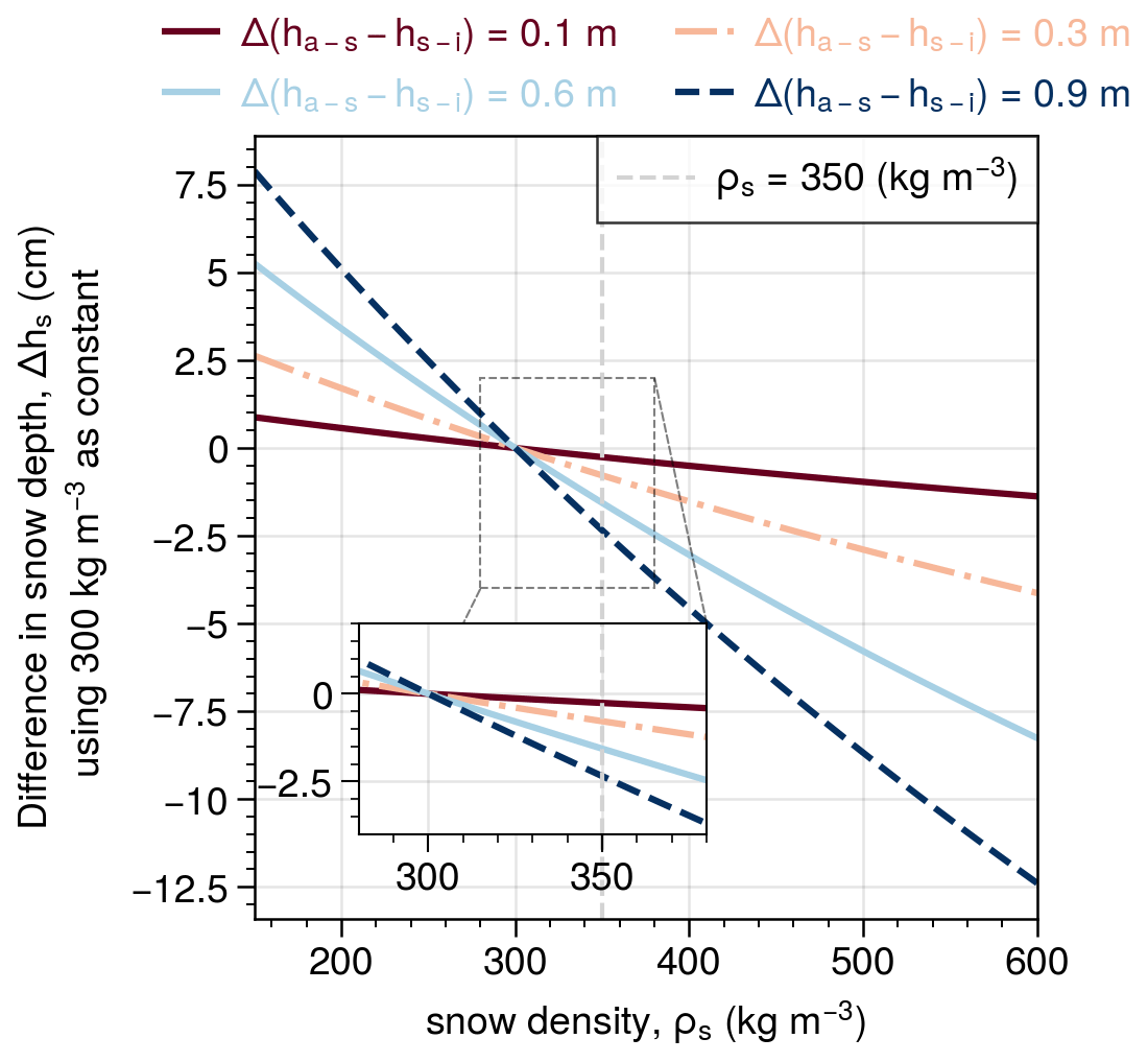
Figure 5Difference in snow depth (Δhs) from using a constant snow density of 300 kg m−3 compared with varying snow densities between 150–600 kg m−3 (based on field data presented in Massom et al., 2001) shown for four examples of height differences between interfaces (Δ(ha-s−hs-i)). An inset for the density range of 280–380 kg m−3 is shown and discussed further in Sect. 3.3.
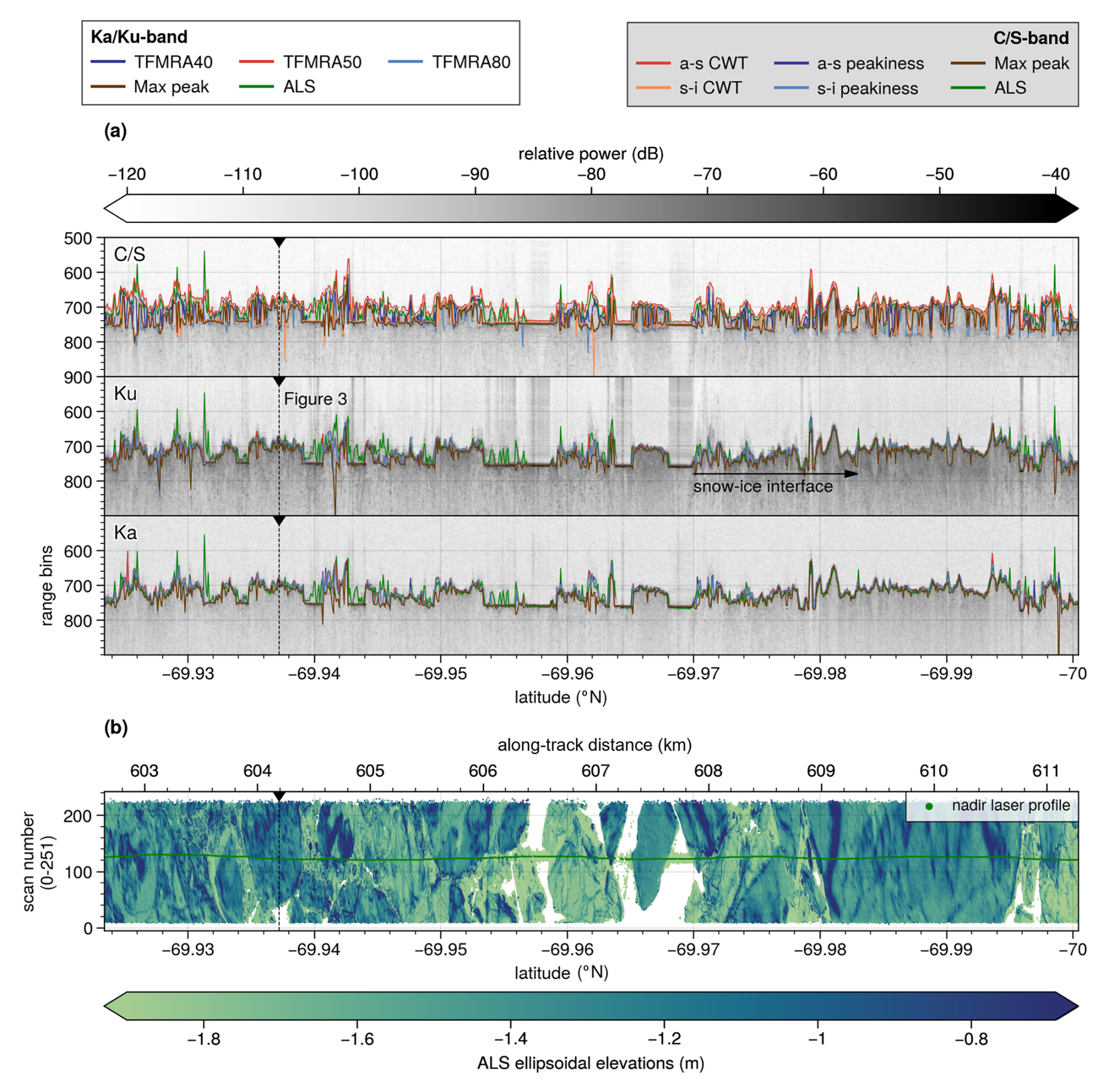
Figure 6(a) Echograms at –band, Ku–band, and Ka-band for the subset with overlaid retracked interfaces for all retrackers. In the Ku-band, what appears to be a s-i interface is somewhat apparent based on a qualitative guess corresponding to the location of the s-i interface observed in -band; however, it does not represent the maximum scatter or somewhere on the leading edge of Ku-band. (b) Corresponding ALS swath and nadir profile are shown as a function of scan number (not projected).
Table 3Comparison between ALS and scattering horizons of -band (snow radar), Ku-band, and Ka-band over floes (observations with surface classification as leads or mixed removed). Here, μ denotes arithmetic mean, σ is the standard deviation, and N is the number of observations (in total, there were floe observations: N=56 020). For the different versions of N, the percentages compared to the original data count (N) are provided in parentheses. We note here that the comparison between ALS and the radars has not accounted for slower wave propagation; thus, we allow for an uncertainty up to 0.1 m (i.e., double the range resolution in snow, which is about 0.04–0.05 m; see Appendix A2 and Table 1). Furthermore, we consider observations above 1.5 m as artefacts, since this would equate to a snow depth of 1.2 m using a density of 300 kg m−3, which is considered towards extreme snow depths (Massom et al., 2001).
4.1 Microwave penetration into the snow
For comparison of the backscatter horizons (interfaces, i.e., a-s or s-i interfaces) and evaluation of penetration capabilities, it is assumed that the ALS observations, due to zero penetration into the snow cover, are used as a reference for the a-s interface. Traditional hypotheses of the radars include Ka-band primarily scattering at the a-s interface, Ku-band at the s-i interface (over cold and dry snow), and that -band tends to reflect at the s-i interface at maximum scattering (e.g., Kurtz et al., 2013; Kwok et al., 2017; Jutila et al., 2022b; Farrell et al., 2012). Furthermore, airborne Ka-band and Ku-band traditionally assume one surface to primarily contribute (thus, we only track one point of the waveform). In contrast, we assume -band to be influenced enough by both interfaces to retrack both. We note that these conditions are not necessarily met during this campaign, with the relatively warm weather conditions. This is further discussed in Sect. 5. To evaluate the full extent of penetration, we here use MAX to present the strongest scatter.
The maximum power was reflected within 0.10 m from the a-s interface (using ALS) for 32.7 % and 42.9 % of the observations at Ku-band and Ka-band, respectively (Table 3), from which 82 %–86 % are coincident with those identified by TFMRA50 (see also Sect. 4.2). This is contrary to the assumption of total penetration at Ku-band scattering at the s-i interface. However, ∼60 % of Ku-band observations using MAX were scattered lower in the snowpack, between 0.1 and 1.5 m, when compared to ALS. Since the a-s interface plays a significant role in the backscattering of the Ku-band radar signal, conventional retrackers used for spaceborne estimates are unable to retrieve all the information available from airborne observations. Instead, the variability of retracked interfaces using MAX provides an indication of how much the contribution varies between interfaces. For comparison, Ka-band MAX is also reflected in the snow in 46 % of the observations assuming ALS represents the a-s interface. This suggests that either (1) the Ka-band is able to penetrate into the snow or (2) the laser and the Ka-band radar are dominated by different scattering interfaces that might provide a deeper snow depth than actually present. Armitage and Ridout (2015) noted that the Ka-band reflects from midway in the snowpack and upwards, which appears to be consistent with several instances here (Fig. 6a, Ka-band).
We observe that the Ku-band occasionally receives MAX reflections further into the snowpack but rarely to the extent seen with the -band. Additionally, there are instances where some s-i interface contribution is visible at Ku-band but only after MAX has been reached (Fig. 6a, Ku-band). This suggests that a-s interfaces (or other internal layers or snow metamorphism) can be the dominating contributor to the waveform but that the s-i interface may be extracted from a less dominant peak. Future work on revisiting retrieval methods where these instances occur under the assumption of multiple interfaces being present is encouraged. For all radar frequency bands, MAX is reflected more than 1.5 m lower than ALS between 1.5 % and 3.7 % of the time (Table 3), with the snow radar reflecting further than 1.5 m into the snowpack more frequently. In several instances, the Ka-band is reflected slightly below the Ku-band (see Fig. 3 or the larger variability in average values between TFMRA retrackers in Fig. 7). This suggests a greater sensitivity to retracking thresholds at Ka-band and indicates that volume scattering may play a role, resulting in more scattering and delay in pulse travel time. These results open up a discussion on whether, beyond footprint size, the frequency and the dominant backscatter mechanisms at airborne scales should be considered and not neglected.
MAX in -band is only reflected above ALS in 5 % of cases and has fewer observations at the same interface as ALS (16.9 %), highlighting its ability to penetrate into the snowpack and primarily reflect at an interface below (Table 3). For the 74 % of cases where MAX in -band extends within the expected snow depth range, also considering the uncertainty of the observations (0.1 to 1.5 m), the average depth below ALS is 0.57 m. In comparison, Ku- and Ka-band MAX within this range has average values of 0.44 and 0.42 m, respectively. If we consider all observations equally (and not disregard observations before or close to the a-s interface), Ku-band MAX reflects about 0.2 m above MAX, and Ka-band MAX reflects an additional 0.1 m further up on average.
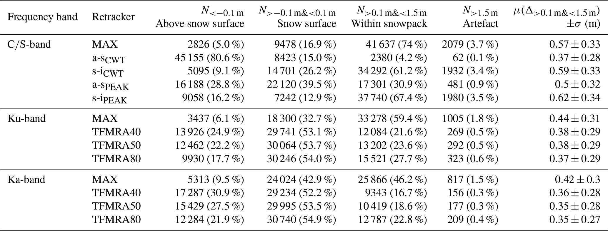
Figure 7(a–c) Comparison between different retrackers as ALS observations (nadir profile), where (a) shows ALS compared with TFMRA at 40 %, 50 %, and 80 % as well as MAX for Ku-band, (b) shows the same as (a) but for Ka-band, and (c) presents the comparison of interfaces identified using PEAK and CWT for -band as well as MAX. Statistics show average and standard deviation, along with 5 %–95 % percentiles. (d–i) Statistics and distribution of snow depth estimations based on the combination of different frequencies, retrackers and interfaces retracked. The percentage in parentheses denotes the number of observations below the threshold value used for statistics on the third line for each distribution. Bin width in panels (a)–(c) is 0.2 and 0.1 m for (d)–(i). The subscript “corr” refers to the applied calibration offset noted in (a)–(c) computed from the manually identified leads and presented in Table 2. Note the different y axis scaling for panels (d)–(i).
4.2 Air–snow and snow–ice: tracing the interfaces
Here, we evaluate the tracked interfaces using conventional assumptions and retrackers applied. It is noticeable that, for the majority of the track, the retrieved elevations for both Ka-band and Ku-band using TFMRA (40, 50 or 80 %) align with the ALS observations (Figs. 6a, 7a–c, and Table 3). This indicates that the first significant peak at both Ka-band and Ku-band is often reflected at the a-s interface. Specifically, between 52 % and 55 % of observations were within 0.1 m of the ALS interface at both Ka-band and Ku-band, using TFMRA for all retracker thresholds (Table 3). In addition, several inconsistencies between elevations from the ALS nadir profile and the radars are observed where the ALS favours scattering from broken floes within open water areas, such as leads, whereas the radar is dominated by the specular reflection (see Fig. 6). Similarly, when highly heterogeneous surfaces occur within the radar footprint, ALS elevations from the same surface show inconsistencies. Thus, the different viewing geometries and sampling of the instruments lead to discrepancies in the surfaces explored (e.g., 9.5 %–30.9 % of the observations at Ka-band and 6.1 %–24.9 % at Ku-band are reflected before the laser scanner, assuming an uncertainty up to 0.1 m).
The impact of a-s interface determination for the snow radar retrackers shows that CWT retracks a surface before the ALS for 80.6 % of the cases (Table 3), as opposed to PEAK, where this occurs in 28.8 % of the cases (following the same tendency as TFMRA for both Ka-band and Ku-band). For both Ku-band and Ka-band, whenever TFMRA retracks a peak that is below the a-s interface (by more than 0.1 m) and within the expected depth range, the averages are ∼0.38 and ∼0.35 m for Ku-band and Ka-band, respectively. However, this applies only for about 16.7 %–27.7 % of cases, depending on retracking threshold used. Were we to consider all observations equally (Fig. 7a–c), TFMRA at all thresholds primarily would retrack the a-s interface within the expected uncertainty of the radar system (maximum deviance from ALS is on average 0.09 m), with CWT a-s primarily retracking above ALS (on average by 0.2 m) and PEAK a-s within 0.01 m from ALS. The CWT s-i interface is retracked ∼0.1 m above the MAX power, whereas PEAK on average retracks s-i ∼0.05 m below MAX.
We note that PEAK has been applied with default parameters based on conditions during an Arctic spring campaign. Ideally, coincident in situ snow depth observations (either from ground-based radars, lidar scanning, or other snow depth estimates) are needed to align the thresholds with the conditions of the current campaign, since waveforms will differ in shape and magnitude depending on radar system and flight altitude. Significant work is required to understand how to tweak PEAK so that both interfaces retrack the expected interfaces. One method would be to align the vertical laser profile with the PEAK a-s interfaces over homogeneous floe surfaces, assuming both instruments are dominated by the same surface conditions and represent the surface similarly. However, this still leaves out how well the s-i interface can be tweaked. Here, in situ observations are crucial. Furthermore, PEAK was originally developed for the 2–18 GHz snow radar system of AWI IceBird, and therefore, the applicability of this method over the 2–8 GHz system may be limited. Although comparing along the radar echogram in Fig. 6 shows that, when clear peaks from the s-i interface are visible, PEAK appears to retrack them, albeit the interface could be retracked some bins before/after MAX is reached, potentially limiting the total snow depth by some range bins. Additional work is required to understand how applicable PEAK is for the 2–8 GHz systems, which could be evaluated from former OIB campaigns whenever additional in situ snow observations are available. Such work is out of the scope of the current study. Nonetheless, using PEAK for 2–8 GHz systems looks promising.
4.3 Deriving airborne snow depths from combinations of retrackers
In total, 16 different combinations of retrieved surfaces with different retrackers and frequencies were investigated for snow depth estimations. Figure 7d presents snow depth computed between ALS and -band (TFMRA50), Ka-band and Ku-band (TFMRA50), or Ka-band and Ku-band (MAX). Here, TFMRA50 generally reflects at or close to the a-s interface (∼ 70 %–76 % of snow depth is below 0.05 m for Ku-band and Ka-band, respectively). Removing these observations provides snow depth on average around 0.25–0.27 m, depending on frequency. Differencing Ka-band and Ku-band to derive snow depth using TFMRA50 or MAX provides limited snow depth (75.14 % and 47.59 % are below 0.05 m). Again, TFMRA50 for both frequency bands appears to primarily (and clearly) reflect the a-s interface, whereas MAX diverges more. At times, Ku-band will have contributions from within the snowpack and/or closer to the s-i interface, resulting in some average snow depths of ∼0.2–0.3 m. However, this average is significantly lower than expected based on the CASSIS model estimates presented in Fig. 1 and the snow radar retrackers (CWT and PEAK, Fig. 7f). Comparing TFMRA50 between the two frequency bands also suggests that the interfaces tracked in of the times (likely the a-s interface) are retrieved more consistently, whereas the contribution to the MAX peak at both frequencies appears to differ more often (average of 0.05 m difference when converting to snow depth, but in almost 50 % of times). Investigating snow depths higher than 0.05 m (range resolution in snow) using Ka-band and Ku-band MAX as the a-s and s-i interfaces, respectively, the average snow depth retrieved is 0.19 m.
Evaluating how MAX compares with ALS provides an idea of how far, at the different frequency bands, the penetration occurs. Here, snow depths using ALS and Ka-band MAX more often represent scattering from the same interface, within 0.05 m from the a-s interface (in almost 46 % of times) compared to Ku-band (∼31 %) and -band (∼17 %); see Fig. 7e. Average snow depths (above 0.05 m) are 0.35, 0.35, and 0.49 m for -band, Ku-band, and Ka-band, respectively. -band extends almost 0.15 m below on average, which supports the assumption and findings of non-complete penetration at Ku-band (and to some extent Ka-band) but rather scattering within the snowpack (whenever it is not reflected at the a-s interface) or limited penetration over thicker snow (Ricker et al., 2015). Interestingly, Ka-band and Ku-band agree within less than a centimetre on average when considering snow depths above 0.05 m, suggesting that (a) they both penetrate into the snowpack and also backscatter at the same interface or that (b) ALS has for these instances identified the a-s interface further above and that this MAX is really reflected at the a-s interface, making these snow depths an artefact of the methods.
To evaluate whether snow depth can be retrieved from both radars individually, we use TFMRA50 as an estimate of the a-s interface and MAX as an estimate of the s-i interface, since this would limit the impact of viewing geometry and provide an idea of whether snow depth can be retrieved for both frequencies under these conditions (see Fig. 7g). Here, more often Ka-band is reflected at the a-s interface with ∼ 44 % having snow depths less than 0.05 m (MAX and TFMRA50 reflected more or less at the same surface), whereas it is ∼ 34.5 % for Ku-band. Considering only the instances where snow depth of more than 0.05 m is achieved, MAX at Ka-band and Ku-band reflects at approximately the same location and provides ∼0.3 m of average snow depth (with Ka-band having slightly higher snow depths, likely due to it being reflected slightly before Ku-band); see Fig. 7g. Using Ka-band at TFMRA50 as the a-s interface and Ku-band at MAX as the s-i interface, in ∼27 % of the cases the snow depth is less than 0.05 m. For the remaining cases, the average snow depth is once again close to 0.3 m. Thus, Ku-band appears unable to extend fully to the s-i interface in many instances when compared with ALS-MAX, but it is reflected on average midway into the snowpack – as is Ka-band. Further work is necessary to evaluate this across other campaigns and in different regions under varying conditions to fully understand its relevance. However, it may also explain why Garnier et al. (2021) observed thinner snow depths from Ka/Ku-band airborne-derived estimates from the Arctic CryoVEx 2017 campaign compared to ALS/Ka from the same campaign.
Applying CWT and PEAK to Ka-band and Ku-band separately to evaluate the potential of extracting snow depth from multiple interfaces by Ka-band or Ku-band alone is presented in Fig. 7h–i. This is particularly interesting, since PEAK is able to retrack the s-i interface at peaks extending beyond MAX. Here, in 35 % of cases, PEAK at Ku-band retrieved snow depths lower than 0.05 m or provides no snow depth information at all, which is in the scale of TFMRA50-MAX at Ku-band. For the snow depths above 0.05 m, averages are around 0.37 m when using PEAK, similar to those obtained by using ALS and MAX at Ku-band. This reflects that, in the majority of cases, PEAK identified the s-i interface at MAX rather than at subsequent, but lower, peaks. For several instances where qualitatively the s-i interface contributes at Ku-band but is not the main scattering interface, PEAK was unable to extract this interface. This is likely due to either the power and right-hand peakiness thresholds applied being too strict for such interfaces to be retracked or additional clutter after the peak would mean that the peak cannot be distinguished as a separate peak. Once more, tweaking of parameters would provide additional insights, granted ground-based observations were available to validate the tweaking.
Using CWT for Ku-band results in ∼10 % of snow depths below 0.05 m and an average of 0.45 m (Fig. 7h). This is interesting, since CWT by definition is not able to retrack peaks below MAX (it only retracks on the leading edge). However, what appears to drive these snow depths is that the a-s interface is retracked significantly before the a-s interface in PEAK, TFMRA in Ku-band at any threshold, and ALS (not shown). As such, while the ranges of snow depths computed using CWT are within expectations and on average follow ALS-MAX well, the estimated location of the interfaces does not necessarily reflect the actual location. For Ka-band, PEAK is only able to extract a snow depth estimate in 40 % of cases, reaching on average ∼0.26 m, which is about 0.1 m thinner than Ku-band. Here, it highlights the lower penetration at Ka-band. Applying CWT at Ka-band also presents higher snow depths (on average 0.37 m, considering only depths above 0.05 m) compared with PEAK which is again counter-intuitive. Along-track comparison over echogram (not shown) also highlights large variability in where the a-s interface is retracked at Ka-band, which could be caused by side lobes that either have not been properly suppressed through deconvolution or larger leading edge at Ka-band caused by a potential higher sensitivity to scattering at this frequency.
Finally, we compare the snow depths retrieved using the PEAK and CWT retrackers for the -band snow radar. Here, clear differences in both shape of distribution and magnitudes of snow depths are evident. CWT rarely observes snow depths of less than 0.05 m (7.10 % of cases), whereas PEAK observes it in ∼36 % of cases (including times when snow depths are not available). On average, CWT retrieves 0.1–0.2 m thicker snow (depending on whether snow depths of less than 0.05 m are included or not). Here, it is clear that the snow radar algorithms show large variation, and further work is necessary to fully understand the limitations of using snow radars over different surfaces. In all cases, the standard deviation of the derived snow depths are of the order of the average snow depths, reflecting the high variability in retrieved snow depths.
The assumptions of Ku-band penetrating the snow cover with a primary scattering horizon at the s-i interface appear not to hold for snow on Antarctic sea ice, especially not during the summer, considering the results herein. Precipitation events (snowfall, rainfall), melting, brine wicking leading to saline snow, and/or flooding due to increased snowfall precipitation and depression of floes may cause the snow to become wet or snow metamorphism to occur (e.g., refreezing, snow-ice formation, ice lenses), which alter the dielectric properties and limits the Ku-band (and Ka-band) penetration. -band appears less impacted by this, as seen by the deeper penetration occurring for -band MAX and the detection of apparent s-i interfaces with both PEAK and CWT at, on average, ∼0.6 m below the a-s interface detected by ALS. For the area of interest (box in Figs. 1, 2b–d), ERA5 simulates average 2 m air temperatures below freezing until after the campaign (since 1 November 2022), although with maximum temperatures reaching thawing temperatures for several instances throughout November (6–7 November, 12–22 November, 25 November–2 December, and 13 December onwards). It is also worth noting that the average temperature up until the campaign occurs is around −5 °C, which could impact the snow and limit the radar penetration as shown by the presence of liquid water in snow at such temperatures (Barber et al., 1995; Kurtz and Farrell, 2011; Kurtz et al., 2013; Rösel et al., 2021). We have not removed data where the air temperature reaches −5 °C or above since the temperature data are based on reanalysis; however, we note that the presence of liquid water in the snowpack would significantly limit Ku-band and Ka-band. Figure 2a shows relatively warm temperatures in the latter part of November, which could have produced a complexly layered snowpack with multiple melt and freeze layers as well as large snow grains. This would limit penetration, especially at higher frequencies. We also note that while a thermal instrument was carried during the campaign and could potentially provide insights into surface temperatures, taking into consideration the field-of-view, the data processing of these data is still underway and can therefore not be evaluated at this time.
Several precipitation events occurred before the campaign which are all identified as snowfall events (Fig. 2a). It is not until after the campaign (16–18 December 2022) that a precipitation event occurs, where the total precipitation is not equal to the snowfall (i.e., a precipitation event with rainfall occurred). Hence, we do not expect a rain-on-snow (ROS) event (e.g., Stroeve et al., 2022) to have occurred or to impact the radar penetration observed along the under-flight. However, there is potential for snowfall events to have depressed the floes and caused flooding, which will impact the scattering horizon (i.e., scattering occurring not at the actual s-i interface but rather above it at the flooded interface, where snow-ice formation could occur), although -band would not be expected to penetrate flooded snow either. However, Marshall et al. (2004) showed for ground-based observations over terrestrial snow that C-band was able to reflect at ground reflections in wet snow, whereas Ku-band was quickly attenuated, which could explain to some extent the limited penetration occurring at both Ku-band and Ka-band. C-band and S-band generally penetrate deeper than Ka-band and Ku-band (with overall dry and cold conditions) due partly to the frequencies of the radar, and they also have potential for penetrating and scattering within the ice cover itself. However, the impact of this is assumed to be negligible for the airborne snow radars and the utilised retrieval methodology, as the maximum scattering at -band snow radars is assumed to be at the s-i interface (e.g., Kwok et al., 2017; Kurtz et al., 2013; Jutila et al., 2022b; Jutila and Haas, 2025; Kurtz and Farrell, 2011; Farrell et al., 2012). Other factors include blow-off of snow from the Filchner–Ronne Ice Shelf or the Antarctic Peninsula through katabatic winds onto the floes may also have increased the snow accumulation on the floes by redistribution of the snow. Additionally, melting of the snowpack when temperatures reach close to positive degrees could lead to scattering further up in the snowpack and result in a detected interface closer to the actual a-s interface along with the potential for superimposed ice to form in which meltwater from the surface will percolate the snowpack towards the s-i interface, resulting in an increased presence of liquid water. It is noticeable that a significant contribution (30 %–42 % for Ku-band and Ka-band, respectively, compared to 17 % at -band) of the maximum power occurs within 0.10 m from the lidar a-s interface, and that Ku-band MAX on average was reflected more than 0.1 m earlier than MAX in -band.
Of particular interest over first-year ice is the impact of brine wicking and a saline snow cover on the radar wave's penetration. Even with the western Weddell Sea sector having been measured to hold up to 80 % multi-year ice (Worby et al., 2008), the overall ice conditions of the Southern Ocean primarily consist of first-year ice. When first-year ice forms, a small amount of brine is expelled upward, yielding a thin layer of brine on the ice surface; with subsequent snow accumulation, an upward wicking of brine via capillary action (Barber et al., 1998; Mallett et al., 2024) into the basal snow layer occurs (Nandan et al., 2017). While this wicking process produces brine-wetted snow which primarily occurs at the base of the snow cover (bottom 6–8 cm) (Nandan et al., 2017), for thicker snow a strong salinity gradient is commonly observed in the bottommost layers and with low brine volumes or brine-free conditions in the uppermost snow layer (Fuller et al., 2014). From a remote sensing perspective, the altering effect of brine on the dielectric and microwave scattering properties of snow is important (Geldsetzer et al., 2009), particularly the strong microwave attenuation within snow volume (Nandan et al., 2016). Large snow grains, due to relatively warm temperatures and coated with brine due to brine wicking, will serve as significant scattering centres from Ku-band radar waves, which could explain some of the limited penetration observed at Ku-band and Ka-band (even when using MAX as s-i interface; see Fig. 7). Sporadic warming events can also amplify the porosity of the ice and its permeability which can further enable upward brine movement (Tucker et al., 1992) and hinder complete microwave penetration to the s-i interface at higher frequencies.
In some of the first studies of airborne CryoVEx Ku-band observations, Hendricks et al. (2010) presented observations from ASIRAS over late-spring western Arctic sea ice and found that little to no penetration into the snow cover occurred over the ice pack, which they concluded showed similarity to Antarctic results found in Willatt et al. (2010) with some regional dependency (comparing results the from Greenland Sea and Lincoln Sea). Here, range was retracked using a threshold spline retracker algorithm, where the spline curve models the leading edge and is used to find the half power point corresponding to the mean surface (analogous to applying TFMRA with 50 %). Similarly to Hendricks et al. (2010), a dominating signal from the a-s interface at both Ka-band and Ku-band is evident for our observations using TFMRA (at any threshold), showing that scattering from the a-s interface plays a significant role (Fig. 7), and further analysis is encouraged for the variety of airborne observations available, considering the different radar systems and their resolutions, as well as seasonal, regional, and hemispheric dependency. In addition, the inconsistency between laser and radar over otherwise expected identical scattering surfaces noted by Hendricks et al. (2010) as also observed here (i.e., over leads; see also Fig. 6) highlights the differences in dominating scattering surfaces for laser and radars. This further complicates the snow depth retrieval when using lidar and radar for different interfaces.
Our results present similar discrepancies between CWT and PEAK as in Jutila et al. (2022b), and similarly to Kwok et al. (2017) a critical question emerges regarding where on the snow radar waveform the a-s and s-i interfaces should be retracked to represent the snow depth correctly. More work is necessary on the snow radars to evaluate when the methods apply, to which extent tweaking of the different thresholds is necessary, how to align methods for different radar systems and campaign conditions (e.g., the impact of low-altitude or high-altitude flights, and Antarctic or Arctic conditions), and what extent the snow radars can fully be used on sea ice and compared to satellites. Our results also show that the assumption of zero freeboard may apply for this campaign along the airborne observations (Fig. 6 for -band shows strong reflections at or even below the surrounding lead surfaces along the selected subset). However, using the snow depth from when the s-i interface occurs below the surrounding lead surface will result in negative freeboards. In particular, negative freeboards can result in flooding of seawater, which can lead to snow-ice formation and additional intrusion of seawater into the snowpack as well as gradual drainage of brine within newly formed snow ice. Such aspects further limit microwave penetration depending on frequency, where Ku-band (and Ka-band in particular) will have limited penetration.
Beyond the microscale impact of the complex snow stratigraphy of the microwave signal, we also need to consider the larger macroscale surface heterogeneity and roughness. Kwok and Maksym (2014) presented a comparison between snow radar (2–8 GHz) Antarctic observations from 2010 and 2011 with derived roughness from airborne lidar (airborne topographic mapper, ATM) observations. Here, roughness was derived as the standard deviation of detrended elevations along a transect of 4 km. They found correlations between average snow depth and surface roughness at 0.77 and 0.84 depending on the years (2010/2011) and locations (Weddell Sea or Bellingshausen Sea), which they conclude is consistent with the fact that deformed ice tends to trap deeper snow. However, while their roughness estimate primarily supported the observation that snow tends to accumulate around obstacles, such a large-scale roughness parameter, this provides little insight into how this, at a point-to-point scale, may impact the retrieved airborne observations. They do note that the snow radar is not able to detect several interfaces over pressure ridges, a similar observation qualitatively made from our observations (see Fig. 6a), where the snow radar is incapable of retrieving snow depth over ridges due to only one single peak being present (as also shown as a waveform example presented in Kurtz et al., 2013).
Hendricks et al. (2010) evaluated airborne Ku-band observations and observed that deformed ice, and thus surface roughness, plays an important role in the retrieved elevations. This has later also been observed for spaceborne observations (e.g., Landy et al., 2020), which also cover a significantly larger area. Hence, roughness at various scales (large-scale deformation or at the scale of wavelengths) impacts the backscatter distribution – and hence the waveform – to an extent that is not well known. In a recent study, De Rijke-Thomas et al. (2023) hypothesise the impact of surface roughness and slope on the backscattering at Ku-band from airborne observations acquired over first-year ice near Eureka during the Arctic spring. They propose that the mechanism, known as probabilistic quasi-specular scattering from the s-i interface, plays a significant role in determining the contributions to radar backscatter distribution at various scales. In particular, an aspect of interest here is the ratio of scattering mechanisms dependent on frequency and, in turn, on the antenna design. Antenna beamwidth is a function of frequency (Table 1), which impacts the shape of the retrieved waveforms and the possibility of detecting individual scattering contributions from different interfaces. The beam-limited footprint is directly proportional to the antenna beamwidth (see Eq. A8), meaning that the -band radar in combination with its antenna beamwidth has a significantly larger beam-limited footprint (∼ 160–550 m) compared to both Ku-band and Ka-band (ranging from ∼ 116 m down to ∼ 80 m) and that potential strong scatters from off-nadir may impact more significantly at -band than at Ka-band. More importantly, the antenna beamwidth along with the individual surface scatters drives the shape of the retrieved waveform, with off-nadir scattering reflected in the trailing edge of the waveform, which could be picked up as s-i interface using the PEAK retracker in the case of strong off-nadir reflections. Or, for snow radars, lower spikes representative of the a-s interface observed before the main spike are, in fact, system artefacts known as side lobes (Kwok and Haas, 2015), which could impact the snow depth retrieval. However, pre-processing steps have been taken to minimise the impact of side lobes (see Appendix A). Nonetheless, it is worth considering what impact antenna beamwidth in combination with frequency has on which interface scattering dominates and how this is reflected in the waveform shape. However, to our knowledge, this has not been evaluated in depth for the radars utilised and is out of the scope of the current study.
From the inconsistent results between radars and retrieval methods presented herein, it is evident that limited conclusions about the most appropriate methods can be derived without the presence of coincident in situ observations. In order to untangle the scattering complexities of snow cover on sea ice, ground-based observations sampled in a manner emulating the airborne systems sensing conditions should be collected to validate the methods and the sensors independently. There is an urgent need for detailed field research and collection; hence, we urge future field campaigns to consider in situ components as a necessity to fully understand the capabilities and limitations of the instruments and their sensing abilities.
In this study, we examined airborne observations from a CRYO2ICE (CryoSat-2 and ICESat-2) under-flight carried out over the Weddell Sea on 13 December 2022 during the CRYO2ICEANT22 campaign. The airborne campaign carried an airborne laser scanner (ALS) and Ka-, Ku-, and -band radars from which snow penetration and potentially snow depth could be derived. This is achieved by utilising four different retrackers (TFMRA at 40 %, 50 %, and 80 %; MAX; CWT; and PEAK), with different retracking thresholds used and by questioning conventional assumptions, in particular regarding whether methodologies applicable to satellites are justified for airborne observations and whether traditionally used retrackers are retrieving what we expect.
At airborne scales, the a-s interface makes a significant contribution at both Ka-band and Ku-band, and this renders retrackers traditionally applied at satellite scales unsuitable for deriving the same surface at airborne scales. Furthermore, Ku-band was incapable of reaching the full extent of the snow radar (and therefore the s-i interface) in the majority of cases. The primary scattering horizon (MAX) at Ku-band and Ka-band was reflected inside the snowpack or at the s-i interface in 60 % and 46 % of times, respectively, whereas at -band MAX was reflected further down into the snowpack (expected at the s-i interface) in 74 % of times. MAX compared with ALS showed penetration down to 0.57 m on average (without accounting for a slower wave propagation speed). Ku-band MAX retracked on average 0.2 m before than -band MAX, and Ka-band retracked even 0.1 m before Ku-band. In contrast, using TFMRA showed scattering at or before the a-s interface in approximately 40 %–70 % of times at Ka-band and Ku-band. Based on these results, future work on evaluating additional Ka- and Ku-band observations from different campaigns is encouraged to understand under which conditions this applies and to which extent we can track different interfaces. Several instances showed primary backscatter at or close to the a-s interface for Ku-band with distinguishable, but lower, scattering from the s-i interface, which could allow for retrieval of snow depth from Ku-band alone. However, a novel retracker to identify these peaks would be necessary, as it would need to not make assumptions on which interface contributes the most at the different frequencies. PEAK was applied as an example of such a retracker; however, several lower peaks were not identified with PEAK, likely due to thresholds that are too strict. Additional tweaking of PEAK would be necessary to understand to what extend it can capture such multiple scattering in snowpacks. Using TFMRA50 (as the a-s interface) and MAX (as the s-i interface) at Ku-band gave similar snow depth results as applying PEAK, supporting conclusions that (a) the a-s interface contributes significantly and is distinguishable as separate peaks and (b) if the main scattering at Ku-band represents the s-i interface, snow depth could be retrieved from such a frequency alone at airborne scale.
The snow radar retracking algorithms (CWT and PEAK) show inconsistencies and discrepancies at -band. CWT retracked the a-s interface before ALS for 80 % of times, whereas PEAK was of the order of TFMRA for Ka-band and Ku-band (around 30 % of observations being reflected before or simply discarded due to no snow observations). The PEAK s-i interface was on average scattered 0.05 m below MAX, whereas the CWT s-i interface scattered 0.2 m before MAX on average. This is expected since PEAK can identify peaks before and after MAX as the s-i interface, provided the peak fulfils the requirements. In comparison, CWT only tracks the location on the leading edge of a waveform as the s-i interface, once it has exceeded a noise + clutter threshold.
Several inconsistencies are observed for the a-s interface determined by ALS and the radars and are likely caused by viewing geometry and different surface scattering mechanisms that dominate the signals. This was particularly evident over leads with broken floes. 5 %–10 % of observations at all frequency bands were reflected before the a-s interface identified by ALS. This further complicates the use of lidar as the a-s interface and any retracked interface as s-i interface from radars. Care should be taken considering highly heterogeneous sea ice cover.
Additional work should be invested to evaluate the snow radar processing methods further and to consider at which point on the snow radar waveforms the a-s and s-i interfaces should be retracked to not only represent the snow depth but also align the location of the derived interfaces with the actual interfaces. The different methods show large inter-variability where the interfaces are retracked depending on waveform shape, as well as snow and ice conditions. For snow depth estimates, CWT on average measured 0.1–0.2 m thicker snow than PEAK. PEAK also shows a stricter requirement to successfully identify snow depth, with more than 36 % of observations discarded or within 0.05 m (identifying the a-s and s-i interfaces at the same peak, resulting in 0 m of snow or discarding waveforms due to too much clutter or too many peaks). Using TFMRA provided limited snow depth information due to primarily scattering at the a-s interface. Using MAX at Ka-band and Ku-band showed higher variability, although still limited penetration. Here, ALS and MAX at Ku-band (and Ka-band) was on average underestimated by at least 0.15 m compared to ALS and MAX, and for several instances, Ka-band and Ku-band reflected either within the snowpack or contributions from different interfaces and attenuation of the signal limits the full extent of penetration. Based on this, it appears that the Ka-band and Ku-band maximum is retrieved from midway in the snow and upwards in the majority of times.
A significant shortcoming of this analysis is the missing validation of the methods and retrievals here, since there are no direct in situ observations available to compare against. Hence, with the significant discrepancies observed between the different methods and combinations of measurements, it is still not clear which combination or method provides observations most consistent with a ground truth. While we acknowledge the significant efforts required to ensure a successful field-based in situ component and that such efforts are often planned but due to unforeseen circumstances cannot be successfully completed, we note that without in situ observations we cannot independently validate the aerial observations nor the satellite observations. This is especially true for underrepresented locations such as the Southern Ocean that has a seasonal dependency that cannot be overlooked. Thus, we urge the continuation of strategically planned field-based efforts necessary to validate the airborne systems, consistently and throughout the season, to ensure that we can properly validate the satellite observations.
Here, the various pre-processing steps of the radar observations are presented. This includes the signal processing applied to generate the radar waveforms used in the study (Appendix A1), the expected radar footprints and resolution (Appendix A2), and the collection of the radar waveforms to provide one track from the segmented data provided by CReSIS for one full flight (Appendix A3).
A1 Signal processing of radar waveforms
Here, we briefly summarise the signal processing applied by CReSIS, also present in different README documents available on the CReSIS FTP server and their website at https://data.cresis.ku.edu/ (last access: 11 September 2024). In addition, for a more in-depth description, the reader is referred to Panzer et al. (2013) and Yan et al. (2017). First, digital errors are set to zero (to minimise digital error effects on processing), and the GPS data are synchronised with the radar observations using the UTC time stored in the radar data files. Next, the analogue-to-digital converter (ADC) input is used to convert from quantisation to voltage, and the direct-current bias is removed by subtracting the mean of the amplitude. Next, quick-look waveforms are generated using unfocused SAR processing for a total of 16 coherent average including hardware and software averages. Next, a fast Fourier transform (FFT) is applied with a Hanning window to convert the raw data into the range domain (analogous to pulse compression), and the data are flipped around based on the Nyquist zone. A high-pass filter is applied in the along-track direction to remove coherent noise. Then, a 1 range-bin by 5 along-track-range-line boxcar filter is applied to the power detected data and then decimated in along-track by 5. The quick-look output is used to find the ice surface location (fully automated and available in the product, but not used for scientific data). Finally, the output is elevation compensated (with radar range bin accuracy) and truncated in fast time based on the data posting settings (here, truncation information is provided; see further processing with this in Sect. A3). Information about the radars are provided in Table 1, and the formulas relevant for deriving footprints and range resolution are presented in Sect. A2.
A2 Resolutions and expected radar footprints
For a flat surface, the range resolution is
where B is the bandwidth, η is the index of refraction for the medium (for air, set to 1), c is the speed of light in vacuum, and kt=1.5 due to the application of a Hanning time-domain window to reduce the range side lobes of the chirped transmit waveform. B can be computed from the parameters f0, fmult, and f1 in the radar observations by the following:
and is 6 GHz for the current CReSIS radars.
Estimate of the along-track resolution before any coherent averaging can be derived similarly to the cross-track resolution. However, a processing known as stacking, coherent averaging, or unfocused SAR processing is applied. The data are coherently averaged 16 times and are decimated by the same amount. Thus, the along-track resolution (σalong-track) is given by
where H is the nominal altitude, λc is the centre frequency, and L is the SAR aperture length can be given as
Assuming all effects are accounted for when coherently averaging the data. However, since the data are only averaged coherently 16 times (sum of hardware and software averaging), we instead compute the SAR aperture length as
where n is the number of averages, v is the velocity of the aircraft, and PRF is the pulse repetition frequency. A factor of 5, equivalent to the number of incoherent integrations after unfocused SAR processing, must be accounted for when deriving the effective SAR aperture length (L) by dividing by 5.
For smooth or quasi-specular targets (such as interfaces), the primary response is from the first Fresnel zone. Thus, the directivity of specular targets effectively creates the appearance of a cross-track resolution equal to this first Fresnel zone. The first Fresnel zone is a circle with a diameter given by
where T is the depth in ice of the target (here assumed 0), and H is the height above the air–snow interface (or here the altitude). However, for rough surfaces with no clear layers, the cross-track resolution is constrained by the pulse-limited footprint, approximately given by
Finally, considering the beam widths and impact of range, the cross-track resolution be computed as beam-limited considering potential off-nadir reflections that could impact the signal:
where β is the beam width in radians. Here, we use the beam width given for the lowest frequency of the radar since beamwidth changes with frequency and is the largest at lowest frequencies.
A3 Processing of CReSIS radar segments into one under-flight track
The CReSIS data are available as .mat files grouped into segments, where one segment is a continuous data set where the radar settings do not change. A day can be divided into segments if the radar settings were changed, hard drives were switched, or other operational constraints required the radar recording to be turned off and on. In addition, each segment is broken into frames (analogous to satellite SAR scenes) to make analysis of the data easier. Frames span 33 s, covering approximately 4–5 km, depending on the aircraft speed. As such, one under-flight will have several frames spanning the segments and the entire under-flight. The CReSIS parameters of interest to this study include radar waveforms (Data in the CReSIS product), flight altitude (Elevation), GPS time (GPS_time), heading (Heading), pitch (Pitch), and roll angle (Roll) of the aircraft, latitude (Latitude), longitude (Longitude), two-way-travel time for a full waveform (Time), and various parameter records (such as f1, f0, and fmult which are necessary to run a retracking algorithm for the snow radar). It may be that the data are truncated (focused only around a clear surface signal to limit data size), where the waveform parameter can be truncated both before and after the identified surface signal. If that is the case, the parameter Truncate_Bins is activated and shows where in the Time parameter the waveform is relative to. This is important to incorporate since if truncation has been activated, the size of the waveform (number of range bins) will differ depending on frames. This plays a role when creating one file for the entire flight as the frames of one flight will change in size (of the waveforms), depending on the truncation occurred and the surface encountered; therefore, the data must be padded somehow to ensure the same parameter size. Furthermore, this allows us to properly estimate the range to a surface depending on the retracked waveform. Whenever the roll angle is more than , the range observation is set to “not-a-number”.
For position estimation, failing to compensate for the lever arm from the inertial measurement unit (IMU) to the GNSS antennas yields an attitude-dependent error (Stovner and Johansen, 2019). Lever arms, which are known locations of the GNSS receivers relative to the IMU, must therefore be used to correct the observations, and are provided in Table B1.
Table B1Lever arms (x, y, z) in metres for the different instruments. x is pointing to nose, y is pointing to the right wing and z is pointing downwards. For corrections, the arithmetic averages of the transmit and receive offsets were used as the offsets of radar phase centres with respect to the GPS. Only Δ in z axis is used to correct when aligning the ranges for visualisation purposes in Fig. 2a, the lever arms have otherwise been corrected for in the actual data.
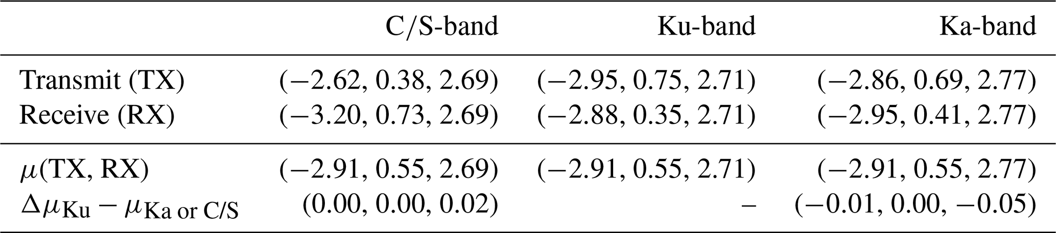
The CRYO2ICEANT22 campaign data are currently in the final stages before approval from ESA and will, once approved, be published on the ESA campaign site and on http://www.cs2eo.org (Bizoń et al., 2025). The processed CRYO2ICEANT22 data presented here are available from DTU DATA under https://doi.org/10.11583/DTU.26732227 (Fredensborg Hansen et al., 2024a). The code for processing the provided CRYO2ICEANT22 data and the satellite/model data are available on the following GitHub repository (Fredensborg Hansen, 2024, https://doi.org/10.5281/zenodo.13749342): https://github.com/reneefredensborg/cryo2iceant22-airborne- cryo2ice-weddell-sea-ice (last access: 11 September 2024).
ERA5 reanalysis data (Hersbach et al., 2023) are available from the Copernicus Climate Change Service (C3S) at https://doi.org/10.24381/cds.adbb2d47.
To generate Fig. 1, the following data have been extracted: the daily output on 13 December 2022 of CASSIS was provided by Isobel R. Lawrence via Andy Ridout (University College London, UCL). Currently, CASSIS model output from 1981–2021 (Lawrence et al., 2024) is available from http://www.cpom.ucl.ac.uk/cassis/ (last access: 9 July 2024). AMSR-E/AMSR2 Unified L3 Daily 12.5 km Brightness Temperatures, Sea Ice Concentration, Motion & Snow Depth Polar Grids, Version 1 (Meier et al., 2018) is available under https://doi.org/10.5067/RA1MIJOYPK3P on NSIDC.
Conceptualisation: RMFH, HS. Data curation: RMFH, JL, FRM, HS, IRL. Formal Analysis: RMFH, HS. Funding acquisition: HS, KVH, RF, JW. Investigation: RMFH, HS, AJ, IRL, SBS, GV. Methodology: RMFH, HS, AJ, IRL, AS, KVH, ER. Project administration: HS, RF, TGDC, JW. Software: RMFH. Supervision: HS, ER, KVH, RF, JW, TGDC. Validation: RMFH. Visualisation: RMFH. Writing (original draft): RMFH. Writing (review & editing): all authors.
The contact author has declared that none of the authors has any competing interests.
Publisher's note: Copernicus Publications remains neutral with regard to jurisdictional claims made in the text, published maps, institutional affiliations, or any other geographical representation in this paper. While Copernicus Publications makes every effort to include appropriate place names, the final responsibility lies with the authors.
This work was supported by ESA with DTU Space CRYO2ICEANT 2022 – Technical Support for the Antarctica CRYO2ICE 2022 Experiment (grant no. 4000141420/23/NL/IB/ab) and the UK Natural Environment Research Council DEFIANT project (grant no. NE/W004747/1). Renée Mie Fredensborg Hansen and Henriette Skourup acknowledge the great discussions of the International Space Science Institute (ISSI) Team 501 – “Multi-Sensor Observations of Antarctic Sea Ice and its Snow Cover”. Renée Mie Fredensborg Hansen was supported by the Nordic5Tech joint PhD-alliance research project between DTU and NTNU to characterise extreme sea ice features with a combination of remote sensing, in situ data, and physical modelling. Arttu Jutila was supported by the Research Council of Finland (grant no. 341550).
We acknowledge the use of data and/or data products from CReSIS generated with support from the University of Kansas, NASA Operation IceBridge (grant no. NNX16AH54G), NSF (grant nos. ACI-1443054, OPP-1739003, and IIS-1838230), Lilly Endowment Incorporated, and Indiana METACyt Initiative.
We thank the crew of the Rothera Research Station and the pilots who made the CRYO2ICEANT2022 campaign possible.
This research has been supported by the European Space Agency (grant no. 4000141420/23/NL/IB/ab), the UK Natural Environment Research Council (NERC) DEFIANT project (no. NE/W004747/1), and the Research Council of Finland (grant no. 341550).
This paper was edited by Vishnu Nandan and reviewed by John Yackel and two anonymous referees.
Armitage, T. W. K. and Ridout, A. L.: Arctic sea ice freeboard from AltiKa and comparison with CryoSat-2 and Operation IceBridge, Geophys. Res. Lett., 42, 6724–6731, https://doi.org/10.1002/2015GL064823, 2015. a, b, c, d
Arndt, S. and Paul, S.: Variability of Winter Snow Properties on Different Spatial Scales in the Weddell Sea, J. Geophys. Res.-Oceans, 123, 8862–8876, https://doi.org/10.1029/2018JC014447, 2018. a
Arndt, S., Haas, C., Meyer, H., Peeken, I., and Krumpen, T.: Recent observations of superimposed ice and snow ice on sea ice in the northwestern Weddell Sea, The Cryosphere, 15, 4165–4178, https://doi.org/10.5194/tc-15-4165-2021, 2021. a
Arndt, S., Maaß, N., Rossmann, L., and Nicolaus, M.: From snow accumulation to snow depth distributions by quantifying meteoric ice fractions in the Weddell Sea, The Cryosphere, 18, 2001–2015, https://doi.org/10.5194/tc-18-2001-2024, 2024. a
Barber, D., Fung, A., Grenfell, T., Nghiem, S., Onstott, R., Lytle, V., Perovich, D., and Gow, A.: The role of snow on microwave emission and scattering over first-year sea ice, IEEE T. Geosci. Remote, 36, 1750–1763, https://doi.org/10.1109/36.718643, 1998. a
Barber, D. G., Reddan, S. P., and LeDrew, E. F.: Statistical characterization of the geophysical and electrical properties of snow on Landfast first-year sea ice, J. Geophys. Res.-Oceans, 100, 2673–2686, https://doi.org/10.1029/94JC02200, 1995. a
Beaven, S. G., Lockhart, G. L., Gogineni, S. P., Hossetnmostafa, A. R., Jezek, K., Gow, A. J., Perovich, D. K., Fung, A. K., and Tjuatja, S.: Laboratory measurements of radar backscatter from bare and snow-covered saline ice sheets, Int. J. Remote Sens., 16, 851–876, https://doi.org/10.1080/01431169508954448, 1995. a
Bizoń, J., Burns, C., Easthope, R., Ewart, M., Goss, T., Gourmelen, N., Horton, A., Incatasciato, A., Jakob, L., Michael, C., Parrinello, T., Bouffard, J., Di Bella, A., and Meloni M.: cs2eo, European Space Agency, http://cs2eo.org (last access: 15 September 2025), 2025. a
Deems, J. S., Painter, T. H., and Finnegan, D. C.: Lidar measurement of snow depth: a review, J. Glaciol., 59, 467–479, https://doi.org/10.3189/2013JoG12J154, 2013. a
De Rijke-Thomas, C., Landy, J. C., Mallett, R., Willatt, R. C., Tsamados, M., and King, J.: Airborne Investigation of Quasi-Specular Ku-Band Radar Scattering for Satellite Altimetry Over Snow-Covered Arctic Sea Ice, IEEE T. Geosci. Remote, 61, 2004919, https://doi.org/10.1109/TGRS.2023.3318263, 2023. a, b, c, d, e, f
Farrell, S. L., Kurtz, N., Connor, L. N., Elder, B. C., Leuschen, C., Markus, T., McAdoo, D. C., Panzer, B., Richter-Menge, J., and Sonntag, J. G.: A First Assessment of IceBridge Snow and Ice Thickness Data Over Arctic Sea Ice, IEEE T. Geosci. Remote, 50, 2098–2111, https://doi.org/10.1109/TGRS.2011.2170843, 2012. a, b
Fons, S. W. and Kurtz, N. T.: Retrieval of snow freeboard of Antarctic sea ice using waveform fitting of CryoSat-2 returns, The Cryosphere, 13, 861–878, https://doi.org/10.5194/tc-13-861-2019, 2019. a, b
Fredensborg Hansen, R. M.: cryo2iceant22-airborne-cryo2ice-weddell-sea-ice, Zenodo [code], https://doi.org/10.5281/zenodo.13749342, 2024. a
Fredensborg Hansen, R. M., Skourup, H., Lawrence, I., Li, J., Rodriguez-Morales, F., and Yi, D.: Airborne ellipsoidal elevations and derived snow depths from Ka-, Ku-, -band and lidar observations along CRYO2ICEANT22 under-flight (13 December 2022) along co-located CRYO2ICE (CryoSat-2 and ICESat-2) observations of snow depth using CryoTEMPO, FF-SAR and ESA-E CryoSat-2 processing chains, Technical University of Denmark [data set], https://doi.org/10.11583/DTU.26732227, 2024a. a
Fredensborg Hansen, R. M., Skourup, H., Rinne, E., Høyland, K. V., Landy, J. C., Merkouriadi, I., and Forsberg, R.: Arctic Freeboard and Snow Depth From Near-Coincident CryoSat-2 and ICESat-2 (CRYO2ICE) Observations: A First Examination of Winter Sea Ice During 2020–2022, Earth Space Sci., 11, e2023EA003313, https://doi.org/10.1029/2023EA003313, 2024b. a
Fredensborg Hansen, R. M., Skourup, H., Rinne, E., Jutila, A., Lawrence, I. R., Shepherd, A., Høyland, K. V., Li, J., Rodriguez-Morales, F., Simonsen, S. B., Wilkinson, J., Veyssiere, G., Yi, D., Forsberg, R., and Casal, T. G. D.: Multi-frequency altimetry snow depth estimates over heterogeneous snow-covered Antarctic summer sea ice – Part 2: Comparing airborne estimates with near-coincident CryoSat-2 and ICESat-2 (CRYO2ICE), The Cryosphere, 19, 4193–4209, https://doi.org/10.5194/tc-19-4193-2025, 2025. a
Fuller, M. C., Geldsetzer, T., Gill, J. P. S., Yackel, J. J., and Derksen, C.: C-band backscatter from a complexly-layered snow cover on first-year sea ice, Hydrol. Process., 28, 4614–4625, https://doi.org/10.1002/hyp.10255, 2014. a
Galin, N., Worby, A., Markus, T., Leuschen, C., and Gogineni, P.: Validation of Airborne FMCW Radar Measurements of Snow Thickness Over Sea Ice in Antarctica, IEEE T. Geosci. Remote, 50, 3–12, https://doi.org/10.1109/TGRS.2011.2159121, 2012. a
Garnier, F., Fleury, S., Garric, G., Bouffard, J., Tsamados, M., Laforge, A., Bocquet, M., Fredensborg Hansen, R. M., and Remy, F.: Advances in altimetric snow depth estimates using bi-frequency SARAL and CryoSat-2 Ka–Ku measurements, The Cryosphere, 15, 5483–5512, https://doi.org/10.5194/tc-15-5483-2021, 2021. a, b, c
Geldsetzer, T., Langlois, A., and Yackel, J.: Dielectric properties of brine-wetted snow on first-year sea ice, Cold Reg. Sci. Technol., 58, 47–56, https://doi.org/10.1016/j.coldregions.2009.03.009, 2009. a
Grosfeld, K., Treffeisen, R., Asseng, J., Bartsch, A., Bräuer, B., Fritzsch, B., Gerdes, R., Hendricks, S., Hiller, W., Heygster, G., Krumpen, T., Lemke, P., Melsheimer, C., Nicolaus, M., Ricker, R., and Weigelt, M.: Online sea-ice knowledge and data platform http://www.meereisportal.de, Polarforschung, 85, 143–155, https://doi.org/10.2312/polfor.2016.011, 2016. a
Guerreiro, K., Fleury, S., Zakharova, E., Rémy, F., and Kouraev, A.: Potential for estimation of snow depth on Arctic sea ice from CryoSat-2 and SARAL/AltiKa missions, Remote Sens. Environ., 186, 339–349, https://doi.org/10.1016/j.rse.2016.07.013, 2016. a
Hendricks, S.: Cryo-TEMPO: Algorithm Theoretical Basis Document – Sea Ice, Version 2.1, https://earth.esa.int/eogateway/documents/20142/37627/Cryo-TEMPO-ATBD-Sea-Ice.pdf (last access: 7 August 2024; currently not available), 2022. a, b
Hendricks, S., Stenseng, L., Helm, V., and Haas, C.: Effects of surface roughness on sea ice freeboard retrieval with an Airborne Ku-Band SAR radar altimeter, in: 2010 IEEE International Geoscience and Remote Sensing Symposium, 2010, Honolulu, HI, USA, 3126–3129, https://doi.org/10.1109/IGARSS.2010.5654350, 2010. a, b, c, d, e
Hersbach, H., Bell, B., Berrisford, P., Biavati, G., Horányi, A., Muñoz Sabater, J., Nicolas, J., Peubey, C., Radu, R., Rozum, I., Schepers, D., Simmons, A., Soci, C., Dee, D., and Thépaut, J.-N.: ERA5 hourly data on single levels from 1940 to present, Copernicus Climate Change Service (C3S) Climate Data Store (CDS) [data set], https://doi.org/10.24381/cds.adbb2d47, 2023. a, b
Jensen, T. E.: iMAR iNAT-RQH-4001, Technical University of Denmark, https://doi.org/10.11583/DTU.25673604.v1, 2024. a
Jutila, A. and Haas, C.: C and K band microwave penetration into snow on sea ice studied with off-the-shelf tank radars, Ann. Glaciol., 65, e5, https://doi.org/10.1017/aog.2023.47, 2025. a
Jutila, A., Hendricks, S., Ricker, R., von Albedyll, L., Krumpen, T., and Haas, C.: Retrieval and parameterisation of sea-ice bulk density from airborne multi-sensor measurements, The Cryosphere, 16, 259–275, https://doi.org/10.5194/tc-16-259-2022, 2022a. a
Jutila, A., King, J., Paden, J., Ricker, R., Hendricks, S., Polashenski, C., Helm, V., Binder, T., and Haas, C.: High-Resolution Snow Depth on Arctic Sea Ice From Low-Altitude Airborne Microwave Radar Data, IEEE T. Geosci. Remote, 60, 4300716, https://doi.org/10.1109/TGRS.2021.3063756, 2022b. a, b, c, d, e, f, g
Kacimi, S. and Kwok, R.: The Antarctic sea ice cover from ICESat-2 and CryoSat-2: freeboard, snow depth, and ice thickness, The Cryosphere, 14, 4453–4474, https://doi.org/10.5194/tc-14-4453-2020, 2020. a, b, c
Kacimi, S. and Kwok, R.: Arctic Snow Depth, Ice Thickness, and Volume From ICESat-2 and CryoSat-2: 2018–2021, Geophys. Res. Lett., 49, e2021GL097448, https://doi.org/10.1029/2021GL097448, 2022. a
Kern, M., Cullen, R., Berruti, B., Bouffard, J., Casal, T., Drinkwater, M. R., Gabriele, A., Lecuyot, A., Ludwig, M., Midthassel, R., Navas Traver, I., Parrinello, T., Ressler, G., Andersson, E., Martin-Puig, C., Andersen, O., Bartsch, A., Farrell, S., Fleury, S., Gascoin, S., Guillot, A., Humbert, A., Rinne, E., Shepherd, A., van den Broeke, M. R., and Yackel, J.: The Copernicus Polar Ice and Snow Topography Altimeter (CRISTAL) high-priority candidate mission, The Cryosphere, 14, 2235–2251, https://doi.org/10.5194/tc-14-2235-2020, 2020. a
King, J., Skourup, H., Hvidegaard, S. M., Rösel, A., Gerland, S., Spreen, G., Polashenski, C., Helm, V., and Liston, G. E.: Comparison of Freeboard Retrieval and Ice Thickness Calculation From ALS, ASIRAS, and CryoSat-2 in the Norwegian Arctic to Field Measurements Made During the N-ICE2015 Expedition, J. Geophys. Res.-Oceans, 123, 1123–1141, https://doi.org/10.1002/2017JC013233, 2018. a, b
King, J., Brady, M., and Newman, T.: kingjml/pySnowRadar: Updated IEEE TGRS Submission, Zenodo [code], https://doi.org/10.5281/zenodo.4071947, 2020. a
Kurtz, N. T. and Farrell, S. L.: Large-scale surveys of snow depth on Arctic sea ice from Operation IceBridge, Geophys. Res. Lett., 38, L20505, https://doi.org/10.1029/2011GL049216, 2011. a, b, c
Kurtz, N. T., Farrell, S. L., Studinger, M., Galin, N., Harbeck, J. P., Lindsay, R., Onana, V. D., Panzer, B., and Sonntag, J. G.: Sea ice thickness, freeboard, and snow depth products from Operation IceBridge airborne data, The Cryosphere, 7, 1035–1056, https://doi.org/10.5194/tc-7-1035-2013, 2013. a, b, c, d
Kwok, R. and Haas, C.: Effects of radar side-lobes on snow depth retrievals from Operation IceBridge, J. Glaciol., 61, 576–584, https://doi.org/10.3189/2015JoG14J229, 2015. a, b
Kwok, R. and Kacimi, S.: Three years of sea ice freeboard, snow depth, and ice thickness of the Weddell Sea from Operation IceBridge and CryoSat-2, The Cryosphere, 12, 2789–2801, https://doi.org/10.5194/tc-12-2789-2018, 2018. a, b
Kwok, R. and Maksym, T.: Snow depth of the Weddell and Bellingshausen sea ice covers from IceBridge surveys in 2010 and 2011: An examination, J. Geophys. Res.-Oceans, 119, 4141–4167, https://doi.org/10.1002/2014JC009943, 2014. a, b, c, d, e
Kwok, R., Kurtz, N. T., Brucker, L., Ivanoff, A., Newman, T., Farrell, S. L., King, J., Howell, S., Webster, M. A., Paden, J., Leuschen, C., MacGregor, J. A., Richter-Menge, J., Harbeck, J., and Tschudi, M.: Intercomparison of snow depth retrievals over Arctic sea ice from radar data acquired by Operation IceBridge, The Cryosphere, 11, 2571–2593, https://doi.org/10.5194/tc-11-2571-2017, 2017. a, b, c, d, e
Kwok, R., Kacimi, S., Webster, M., Kurtz, N., and Petty, A.: Arctic Snow Depth and Sea Ice Thickness From ICESat-2 and CryoSat-2 Freeboards: A First Examination, J. Geophys. Res.-Oceans, 125, e2019JC016008, https://doi.org/10.1029/2019JC016008, 2020. a
Landy, J. C., Petty, A. A., Tsamados, M., and Stroeve, J. C.: Sea Ice Roughness Overlooked as a Key Source of Uncertainty in CryoSat-2 Ice Freeboard Retrievals, J. Geophys. Res.-Oceans, 125, e2019JC015820, https://doi.org/10.1029/2019JC015820, 2020. a
Landy, J. C., Bouffard, J., Wilson, C., Rynders, S., Aksenov, Y., and Tsamados, M.: Improved Arctic Sea Ice Freeboard Retrieval From Satellite Altimetry Using Optimized Sea Surface Decorrelation Scales, J. Geophys. Res.-Oceans, 126, e2021JC017466, https://doi.org/10.1029/2021JC017466, 2021. a
Lawrence, I. R., Tsamados, M. C., Stroeve, J. C., Armitage, T. W. K., and Ridout, A. L.: Estimating snow depth over Arctic sea ice from calibrated dual-frequency radar freeboards, The Cryosphere, 12, 3551–3564, https://doi.org/10.5194/tc-12-3551-2018, 2018. a
Lawrence, I. R., Ridout, A. L., Shepherd, A., and Tilling, R.: A Simulation of Snow on Antarctic Sea Ice Based on Satellite Data and Climate Reanalyses, J. Geophys. Res.-Oceans, 129, e2022JC019002, https://doi.org/10.1029/2022JC019002, 2024 (data available at: http://www.cpom.ucl.ac.uk/cassis/, last access: 9 July 2024). a, b
MacGregor, J. A., Boisvert, L. N., Medley, B., Petty, A. A., Harbeck, J. P., Bell, R. E., Blair, J. B., Blanchard-Wrigglesworth, E., Buckley, E. M., Christoffersen, M. S., Cochran, J. R., Csathó, B. M., De Marco, E. L., Dominguez, R. T., Fahnestock, M. A., Farrell, S. L., Gogineni, S. P., Greenbaum, J. S., Hansen, C. M., Hofton, M. A., Holt, J. W., Jezek, K. C., Koenig, L. S., Kurtz, N. T., Kwok, R., Larsen, C. F., Leuschen, C. J., Locke, C. D., Manizade, S. S., Martin, S., Neumann, T. A., Nowicki, S. M., Paden, J. D., Richter-Menge, J. A., Rignot, E. J., Rodríguez-Morales, F., Siegfried, M. R., Smith, B. E., Sonntag, J. G., Studinger, M., Tinto, K. J., Truffer, M., Wagner, T. P., Woods, J. E., Young, D. A., and Yungel, J. K.: The Scientific Legacy of NASA’s Operation IceBridge, Rev. Geophys., 59, e2020RG000712, https://doi.org/10.1029/2020RG000712, 2021. a, b, c
Mallett, R., Nandan, V., Stroeve, J., Willatt, R., Saha, M., Yackel, J., Veysière, G., and Wilkinson, J.: Dye tracing of upward brine migration in snow, Ann. Glaciol., 65, e26, https://doi.org/10.1017/aog.2024.27, 2024. a
Mallett, R. D. C., Lawrence, I. R., Stroeve, J. C., Landy, J. C., and Tsamados, M.: Brief communication: Conventional assumptions involving the speed of radar waves in snow introduce systematic underestimates to sea ice thickness and seasonal growth rate estimates, The Cryosphere, 14, 251–260, https://doi.org/10.5194/tc-14-251-2020, 2020. a
Marshall, H., Koh, G., and Forster, R. R.: Ground‐based frequency‐modulated continuous wave radar measurements in wet and dry snowpacks, Colorado, USA: an analysis and summary of the 2002–03 NASA CLPX data, Hydrol. Process., 18, 3609–3622, https://doi.org/10.1002/hyp.5804, 2004. a
Massom, R. A., Eicken, H., Hass, C., Jeffries, M. O., Drinkwater, M. R., Sturm, M., Worby, A. P., Wu, X., Lytle, V. I., Ushio, S., Morris, K., Reid, P. A., Warren, S. G., and Allison, I.: Snow on Antarctic sea ice, Rev. Geophys., 39, 413–445, https://doi.org/10.1029/2000RG000085, 2001. a, b, c, d, e, f
Meier, W. N. and Stewart, J. S.: Arctic and Antarctic Regional Masks for Sea Ice and Related Data Products, Version 1, https://doi.org/10.5067/CYW3O8ZUNIWC, 2023. a
Meier, W. N., Markus, T., and Comiso, J. C.: AMSR-E/AMSR2 Unified L3 Daily 12.5 km Brightness Temperatures, Sea Ice Concentration, Motion & Snow Depth Polar Grids. (AU_SI12, Version 1), Boulder, Colorado USA, NASA National Snow and Ice Data Center Distributed Active Archive Center [data set], https://doi.org/10.5067/RA1MIJOYPK3P, 2018. a
Nab, C., Mallett, R., Gregory, W., Landy, J., Lawrence, I., Willatt, R., Stroeve, J., and Tsamados, M.: Synoptic Variability in Satellite Altimeter-Derived Radar Freeboard of Arctic Sea Ice, Geophys. Res. Lett., 50, e2022GL100696, https://doi.org/10.1029/2022GL100696, 2023. a
Nandan, V., Geldsetzer, T., Islam, T., Yackel, J. J., Gill, J. P., Fuller, M. C., Gunn, G., and Duguay, C.: Ku-, X- and C-band measured and modeled microwave backscatter from a highly saline snow cover on first-year sea ice, Remote Sens. Environ., 187, 62–75, https://doi.org/10.1016/j.rse.2016.10.004, 2016. a
Nandan, V., Geldsetzer, T., Yackel, J., Mahmud, M., Scharien, R., Howell, S., King, J., Ricker, R., and Else, B.: Effect of Snow Salinity on CryoSat-2 Arctic First-Year Sea Ice Freeboard Measurements, Geophys. Res. Lett., 44, 10419–10426, https://doi.org/10.1002/2017GL074506, 2017. a, b, c
Nandan, V., Scharien, R. K., Geldsetzer, T., Kwok, R., Yackel, J. J., Mahmud, M. S., Rösel, A., Tonboe, R., Granskog, M., Willatt, R., Stroeve, J., Nomura, D., and Frey, M.: Snow Property Controls on Modeled Ku-Band Altimeter Estimates of First-Year Sea Ice Thickness: Case Studies From the Canadian and Norwegian Arctic, IEEE J. Sel. Top. Appl. Earth Obs., 13, 1082–1096, https://doi.org/10.1109/JSTARS.2020.2966432, 2020. a
Nandan, V., Willatt, R., Mallett, R., Stroeve, J., Geldsetzer, T., Scharien, R., Tonboe, R., Yackel, J., Landy, J., Clemens-Sewall, D., Jutila, A., Wagner, D. N., Krampe, D., Huntemann, M., Mahmud, M., Jensen, D., Newman, T., Hendricks, S., Spreen, G., Macfarlane, A., Schneebeli, M., Mead, J., Ricker, R., Gallagher, M., Duguay, C., Raphael, I., Polashenski, C., Tsamados, M., Matero, I., and Hoppmann, M.: Wind redistribution of snow impacts the Ka- and Ku-band radar signatures of Arctic sea ice, The Cryosphere, 17, 2211–2229, https://doi.org/10.5194/tc-17-2211-2023, 2023. a
Newman, T., Farrell, S. L., Richter-Menge, J., Connor, L. N., Kurtz, N. T., Elder, B. C., and McAdoo, D.: Assessment of radar-derived snow depth over Arctic sea ice, J. Geophys. Res.-Oceans, 119, 8578–8602, https://doi.org/10.1002/2014JC010284, 2014. a, b, c, d
Panzer, B., Gomez-Garcia, D., Leuschen, C., Paden, J., Rodriguez-Morales, F., Patel, A., Markus, T., Holt, B., and Gogineni, P.: An ultra-wideband, microwave radar for measuring snow thickness on sea ice and mapping near-surface internal layers in polar firn, J. Glaciol., 59, 244–254, https://doi.org/10.3189/2013JoG12J128, 2013. a, b, c
Ricker, R., Hendricks, S., Helm, V., Skourup, H., and Davidson, M.: Sensitivity of CryoSat-2 Arctic sea-ice freeboard and thickness on radar-waveform interpretation, The Cryosphere, 8, 1607–1622, https://doi.org/10.5194/tc-8-1607-2014, 2014. a, b, c, d
Ricker, R., Hendricks, S., Perovich, D. K., Helm, V., and Gerdes, R.: Impact of snow accumulation on CryoSat-2 range retrievals over Arctic sea ice: An observational approach with buoy data, Geophys. Res. Lett., 42, 4447–4455, https://doi.org/10.1002/2015GL064081, 2015. a
Rodriguez-Morales, F., Gogineni, S., Leuschen, C. J., Paden, J. D., Li, J., Lewis, C. C., Panzer, B., Gomez-Garcia Alvestegui, D., Patel, A., Byers, K., Crowe, R., Player, K., Hale, R. D., Arnold, E. J., Smith, L., Gifford, C. M., Braaten, D., and Panton, C.: Advanced Multifrequency Radar Instrumentation for Polar Research, IEEE T. Geosci. Remote, 52, 2824–2842, https://doi.org/10.1109/TGRS.2013.2266415, 2014. a
Rodriguez-Morales, F., Leuschen, C., Carabajal, C. L., Paden, J., Wolf, J. A., Garrison, S., and McDaniel, J. W.: An Improved UWB Microwave Radar for Very Long-Range Measurements of Snow Cover, IEEE T. Instrum. Meas., 69, 7761–7772, https://doi.org/10.1109/TIM.2020.2982813, 2020. a
Rodríguez-Morales, F., Li, J., Alvestegui, D. G.-G., Shang, J., Arnold, E. J., Leuschen, C. J., Larsen, C. F., Shepherd, A., Hvidegaard, S. M., and Forsberg, R.: A Compact, Reconfigurable, Multi-UWB Radar for Snow Thickness Evaluation and Altimetry: Development and Field Trials, IEEE J. Sel. Top. Appl. Earth Obs., 14, 6755–6765, https://doi.org/10.1109/JSTARS.2021.3092313, 2021. a
Rösel, A., Farrell, S. L., Nandan, V., Richter-Menge, J., Spreen, G., Divine, D. V., Steer, A., Gallet, J.-C., and Gerland, S.: Implications of surface flooding on airborne estimates of snow depth on sea ice, The Cryosphere, 15, 2819–2833, https://doi.org/10.5194/tc-15-2819-2021, 2021. a, b, c
Skourup, H., Simonsen, S. B., Otosaka, I., Fredensborg Hansen, R. M., Shepherd, A., Li, J., Rodriguez-Morales, F., Lawrence, I., Veyssiere, G., and Forsberg, R.: ESA CRYO2ICEEX & NERC DEFIANT – Antarctica 2022. Airborne and in situ field campaign – Final report, Technical University of Denmark, ESA contract report, Version 1, 2024. a
Stovner, B. N. and Johansen, T. A.: GNSS-antenna lever arm compensation in aided inertial navigation of UAVs, in: 2019 18th European Control Conference (ECC), 2019, Naples, Italy, 4040–4046, https://doi.org/10.23919/ECC.2019.8795760, 2019. a
Stroeve, J., Nandan, V., Willatt, R., Dadic, R., Rostosky, P., Gallagher, M., Mallett, R., Barrett, A., Hendricks, S., Tonboe, R., McCrystall, M., Serreze, M., Thielke, L., Spreen, G., Newman, T., Yackel, J., Ricker, R., Tsamados, M., Macfarlane, A., Hannula, H.-R., and Schneebeli, M.: Rain on snow (ROS) understudied in sea ice remote sensing: a multi-sensor analysis of ROS during MOSAiC (Multidisciplinary drifting Observatory for the Study of Arctic Climate), The Cryosphere, 16, 4223–4250, https://doi.org/10.5194/tc-16-4223-2022, 2022. a
Sturm, M., Holmgren, J., and Perovich, D. K.: Winter snow cover on the sea ice of the Arctic Ocean at the Surface Heat Budget of the Arctic Ocean (SHEBA): Temporal evolution and spatial variability, J. Geophys. Res.-Oceans, 107, 8047, https://doi.org/10.1029/2000JC000400, 2002. a
Tilling, R. L., Ridout, A., and Shepherd, A.: Estimating Arctic sea ice thickness and volume using CryoSat-2 radar altimeter data, Adv. Space Res., 62, 1203–1225, https://doi.org/10.1016/j.asr.2017.10.051, 2018. a, b, c, d
Tucker III, W. B., Perovich, D. K., Gow, A. J., Weeks, W. F., and Drinkwater, M. R.: Physical Properties of Sea Ice Relevant to Remote Sensing, American Geophysical Union (AGU), Chap. 2, 9–28, https://doi.org/10.1029/GM068p0009, ISBN 9781118663950, 1992. a
Ulaby, F., Moore, R. K., and Fung, A. K.: Microwave remote sensing: From theory to applications (vol. 3), Norwood, MA., Artech House, 1986. a
Webster, M., Gerland, S., Holland, M., Hunke, E. C., Kwok, R., Lecomte, O., Massom, R., Perovich, D., and Sturm, M.: Snow in the Changing Sea-ice System, Nat. Clim. Change, 8, 946–953, https://doi.org/10.1038/s41558-018-0286-7, 2018. a, b
Willatt, R., Giles, K., Laxon, S., Stone-Drake, L., and Worby, A.: Field Investigations of Ku-Band Radar Penetration Into Snow Cover on Antarctic Sea Ice, IEEE T. Geosci. Remote, 48, 365–372, https://doi.org/10.1109/TGRS.2009.2028237, 2010. a, b
Willatt, R., Laxon, S., Giles, K., Cullen, R., Haas, C., and Helm, V.: Ku-band radar penetration into snow cover on Arctic sea ice using airborne data, Ann. Glaciol., 52, 197–205, https://doi.org/10.3189/172756411795931589, 2011. a, b
Willatt, R., Stroeve, J. C., Nandan, V., Newman, T., Mallett, R., Hendricks, S., Ricker, R., Mead, J., Itkin, P., Tonboe, R., Wagner, D. N., Spreen, G., Liston, G., Schneebeli, M., Krampe, D., Tsamados, M., Demir, O., Wilkinson, J., Jaggi, M., Zhou, L., Huntemann, M., Raphael, I. A., Jutila, A., and Oggier, M.: Retrieval of Snow Depth on Arctic Sea Ice From Surface-Based, Polarimetric, Dual-Frequency Radar Altimetry, Geophys. Res. Lett., 50, e2023GL104461, https://doi.org/10.1029/2023GL104461, 2023. a, b
Worby, A. P., Geiger, C. A., Paget, M. J., Van Woert, M. L., Ackley, S. F., and DeLiberty, T. L.: Thickness distribution of Antarctic sea ice, J. Geophys. Res.-Oceans, 113, C05S92, https://doi.org/10.1029/2007JC004254, 2008. a, b
Yan, J.-B., Gomez-García Alvestegui, D., McDaniel, J. W., Li, Y., Gogineni, S., Rodriguez-Morales, F., Brozena, J., and Leuschen, C. J.: Ultrawideband FMCW Radar for Airborne Measurements of Snow Over Sea Ice and Land, IEEE T. Geosci. Remote, 55, 834–843, https://doi.org/10.1109/TGRS.2016.2616134, 2017. a, b
Zygmuntowska, M., Khvorostovsky, K., Helm, V., and Sandven, S.: Waveform classification of airborne synthetic aperture radar altimeter over Arctic sea ice, The Cryosphere, 7, 1315–1324, https://doi.org/10.5194/tc-7-1315-2013, 2013. a
- Abstract
- Introduction
- Data
- Methodology
- Results
- Discussion and outlook
- Conclusions
- Appendix A: Pre-processing of CReSIS radar observations
- Appendix B: Lever arms
- Code and data availability
- Author contributions
- Competing interests
- Disclaimer
- Acknowledgements
- Financial support
- Review statement
- References