Gravity-derived Antarctic bathymetry using the Tomofast-x open-source code: a case study of Vincennes Bay

Vincennes Bay is a region of East Antarctica that is vulnerable to sub-ice-shelf basal melting from warm ocean water intrusions. The sub-ice-shelf bathymetry in this region is largely unknown despite its importance for ocean dynamics within ice shelf cavities and associated sub-ice-shelf basal melting. Here, we present an open-source approach to deriving open-ocean and sub-ice-shelf bathymetry from airborne gravity data using the Tomofast-x inversion platform. Using existing datasets of bed topography, bathymetry, ice geometry, instrumented seal dives, and airborne gravity data, we perform a constrained gravity inversion to generate a new bathymetry for Vincennes Bay. Our new bathymetry reveals large-scale bathymetric features, some of which were previously known to exist but were not resolved in existing regional bathymetry datasets, including the deep marine trough recently mapped offshore the Vanderford Glacier. A smaller and previously unknown bathymetric trough that reaches depths of more than 1500 m offshore the Adams Glacier is also identified. Ocean modelling using the new bathymetry simulates a 37 % increase in sub-ice-shelf melt rates compared with estimates generated using existing regional bathymetry datasets, highlighting the importance of more accurate bathymetry estimates in this region.

1 Introduction

Around Antarctica, sub-ice-shelf bathymetry exerts an important control on ocean dynamics within ice shelf cavities, with implications for sub-ice-shelf basal melting, grounding line dynamics, and overall ice sheet stability (Liu et al., 2024; McCormack et al., 2024; Haigh et al., 2023; Vaňková et al., 2023; Sun et al., 2022; Goldberg et al., 2020; Gwyther et al., 2014). Offshore, large-scale bathymetric features control the access of warm Circumpolar Deep Water (CDW) onto the continental shelf and towards ice shelf cavities (Eisermann et al., 2024; Liu et al., 2022). In regions of West Antarctica and the Antarctic Peninsula, particularly the Amundsen and Bellingshausen Seas, intrusions of modified Circumpolar Deep Water (mCDW, i.e. relatively warm and salty water) into ice shelf cavities are responsible for widespread grounding line retreat and ice shelf thinning (e.g. Pritchard et al., 2012; Thoma et al., 2008). In regions of East Antarctica, in particular the Sabrina Coast, the presence of mCDW across the continental shelf likely also drives grounding line retreat and mass loss from large outlet glaciers (e.g. Totten, Moscow University, and Denman Glaciers; Ribeiro et al., 2021; Brancato et al., 2020; Greene et al., 2017; Silvano et al., 2016; Rintoul et al., 2016; Li et al., 2015). Given the dominant role of sub-ice-shelf basal melt in mass loss from Antarctica and the control of bathymetry on the access of warm water parcels to ice shelf cavities, it is clear that accurate knowledge of bathymetry is required to improve estimates of basal melt.

Despite its importance, bathymetry on the continental shelf and beneath ice shelves is sparsely sampled and generally poorly resolved. Regional ocean models commonly use continent-wide bathymetry datasets that rely on interpolation of sparse ship-based measurements (e.g. IBCSO v2), with sub-ice-shelf bathymetry typically interpolated between open-ocean measurements and grounded ice topography (Dorschel et al., 2022). Where glacially incised troughs exist adjacent to ice shelf cavities (such as below Vanderford Glacier), IBCSO v2 uses artificial steering lines to model the continuation of these troughs (Dorschel et al., 2022). On the continental shelf, single beam or multibeam echo sounder measurements provide high-accuracy mapping of open-water bathymetry; however, logistical constraints and sea ice cover often limit the spatial extent of such ship-based measurements, particularly in nearshore coastal Antarctica. To date, only 23 % of the Southern Ocean has been mapped (Dorschel et al., 2022), with even fewer observations on the continental shelf around Antarctica. Direct measurements of sub-ice-shelf bathymetry are often impractical, costly, and time-consuming. For example, although seismic sounding and the use of autonomous underwater vehicles can provide direct measurements of sub-ice-shelf bathymetry (e.g. Schmidt et al., 2023; Muto et al., 2013; Smith et al., 2020; Gwyther et al., 2020; Jenkins et al., 2010; Nicholls et al., 2006), these observations are often sparse (e.g. due to access restrictions) and can be of limited quality (e.g. due to heavy crevassing interfering with the signal). Recent bathymetric mapping of a deep marine trough offshore the Vanderford Glacier (Commonwealth of Australia, 2022) provides one example of where large discrepancies exist in regional bathymetry datasets, with the recently mapped bathymetry being up to 1890 m deeper than the existing IBCSO v2 estimate. This highlights the need for alternate methods of deriving both open-ocean and sub-ice-shelf bathymetry.

Inversion of airborne gravity data can provide a first-order estimate of bathymetry, offering an efficient approach to infer sub-ice-shelf and open-ocean bathymetry across large areas, albeit at a lower resolution than ship-based observations. Numerous studies have used gravity inversion to infer bathymetry around Antarctica and Greenland (e.g. Charrassin et al., 2025; Constantino and Tinto, 2023; Eisermann et al., 2021; Yang et al., 2021; Constantino et al., 2020; Eisermann et al., 2020; Jordan et al., 2020; Tinto et al., 2015), with many using proprietary software packages to complete 2D and 3D gravity inversions. While proprietary software packages (e.g. Oasis Montaj and VPmg) provide a convenient approach to performing gravity inversion, the underlying codebase is often inaccessible, resulting in a “black-box” application to inversion problems, which may limit the reproducibility of results. With a move towards “Open Research” (Wilkinson et al., 2016), an open-source solution to the application of gravity inversion to derive bathymetry around the periphery of Antarctica would provide more transparent methodologies, increased reproducibility of analysis, and increased accessibility without software costs. Available open-source geophysical inversion platforms are summarised by Ogarko et al. (2024); however, we are not aware of any existing application of these software packages to Antarctica.

The primary aim of this study is to demonstrate the applicability of Tomofast-x (Ogarko et al., 2024), an open-source geophysical inversion platform, to derive sub-ice-shelf and open-ocean bathymetry from airborne gravity data and to apply this method to the Vincennes Bay region of East Antarctica. A secondary aim is to assess the impact of the updated bathymetry on warm water pathways and sub-ice-shelf basal melt across Vincennes Bay. Following an overview of gravity inversion and a description of applicable features of Tomofast-x in Sect. 2, we introduce the Vincennes Bay study area and provide details on airborne gravity data, the model setup, and a priori information used as input to our gravity inversions (Sect. 3). In Sect. 4, we present a synthetic application (hereafter referred to as the “Synthetic model”) to demonstrate the applicability of Tomofast-x to derive bathymetry and provide details of a quantitative ensemble modelling approach used to identify optimal model parameter choices. In Sect. 5, we subsequently use Tomofast-x to derive sub-ice-shelf and open-ocean bathymetry across Vincennes Bay in East Antarctica (hereafter referred to as the “Vincennes Bay model”), compare the new bathymetry to other current estimates, and discuss model uncertainty. In Sect. 6, we discuss the results and consider the implications for processes relevant to ice sheet retreat, including potential warm water pathways and ocean model-derived melt rates. Finally, we provide a conclusion of this work and comment on the future outlook for improving bathymetry estimates around Antarctica in Sect. 7.

2 Gravity inversions with Tomofast-x

2.1 Overview of gravity inversion

Forward modelling is used to derive a given data field from a model of known physical properties. Conversely, inverse modelling is the process by which physical properties of the Earth are inferred from observational data. Gravity inversion relies on leveraging measured anomalies in the Earth's gravitational field (relative to some assumed theoretical normal mathematical model of gravity) to infer information about the structure of the Earth (e.g. the subsurface mass distribution and topographical features). Anomalies in the Earth's gravitational field arise due to variations in the internal mass distribution of the Earth. Locally, the gravity field is affected by geometry/topography (i.e. volumetric changes) or changes in subsurface densities as well as far-field influences from deep geologic sources. As a result, gravity inversion problems are ill-posed; that is, they present non-unique solutions since comparable gravity responses can be produced by multiple mass distributions.

Two primary approaches to inverse gravity modelling exist: (1) geometry inversions aim to recover the depth and volume of features, while (2) property inversions aim to recover explicit density distributions. Property inversions are commonly used in mineral exploration and structural geological investigations to identify density variations in the subsurface (e.g. Martin et al., 2025; Witter et al., 2016) and have been used within Antarctica to infer crustal structure (e.g. Tondi et al., 2023). Within cryospheric sciences, geometry inversions are commonly applied to derive sub-ice-shelf bathymetry and have also been used to infer Moho depths (e.g. Pappa et al., 2019) and map sedimentary basins across Antarctica (e.g. Aitken et al., 2016). Geometry inversions typically require density values to be defined across the model domain, often relying on simplifying assumptions and requiring careful processing of observed gravity anomalies.

Various approaches to deriving sub-ice-shelf bathymetry have been applied in polar environments, with different considerations of subsurface density variations. For example, Boghosian et al. (2015) completed a series of 2D geometry inversions along gravity flight lines for a number of Greenland fjords. Using reference densities from close to the grounding line, Boghosian et al. (2015) assume homogeneous subsurface densities and assess model uncertainty arising from the choice of reference densities as well as the presence of heterogeneous densities in the form of sediment cover. Similarly, Tinto and Bell (2011); Tinto et al. (2015), Cochran et al. (2014), and Constantino et al. (2020); Constantino and Tinto (2023) conduct 2D geometry inversions along gravity flight lines; however, bedrock densities along the flight lines are manually adjusted to reduce gravity misfits (i.e. the difference between observed and modelled gravity fields). Three-dimensional gravity inversions have been used in various regions, with some studies using a priori information to infer subsurface density variations (e.g. Eisermann et al., 2020, 2021), while others assume homogeneous subsurface densities (e.g. Eisermann et al., 2024; Yang et al., 2021; Millan et al., 2020, 2017; Muto et al., 2013). In this study, we conduct a three-dimensional gravity inversion and assume homogeneous subsurface densities. We discuss the associated limitations of this assumption in Sect. 6.3.

Another important consideration in the application of gravity inversion modelling is the processing of observational gravity datasets. The gravitational field is a function of the cumulative effect of all subsurface mass, including deep geologic structures such as variations in the Moho, shallower topographic features, and variations in subsurface density, such as the presence of sedimentary basins. Therefore, separation of these signals is of paramount importance to ensure the signal of interest (in this case, shallow topographic features) is used as input to the inversion. To isolate the signal from bathymetric features, long-wavelength gravity contributions from deep geologic structures and short-wavelength contributions from local density variations typically need to be removed from the gravity signal (or accounted for explicitly in the inversion model). Often, a “regional” field is estimated and subtracted from the observed gravitational field to return the “residual” field of interest in a process referred to as “regional/residual separation”. Common techniques to estimate regional fields involve low-pass filtering (e.g. Constantino and Tinto, 2023; Eisermann et al., 2021; Cochran et al., 2014), upward continuation of gravity observations (e.g. Tinto et al., 2015), or a DC shift (i.e. constant offset) applied to gravity observations (e.g. An et al., 2019). Alternatively, deep geologic structures (i.e. the Moho) can be included in inversion models to explicitly model these long-wavelength contributions (e.g. Constantino et al., 2020; Greenbaum et al., 2015). Accounting for local density variations is more challenging and often requires iteration between geometry and property inversions to make some inference about lateral density variations. An additional approach that is commonly used can account for both long-wavelength regional gravity contributions and local density variations by calculating gravity misfits (i.e. the difference between observed and modelled gravity signals) in regions of known topography/geometry using forward modelling (e.g. Yang et al., 2021; Jordan et al., 2020; An et al., 2019). Subsequent gravity misfits are interpolated across regions without topographic constraints, and the estimated misfit field is then removed from gravity observations, attenuating unwanted contributions and revealing the best estimate of contributions solely from shallow topographic features. We use this approach of interpolated gravity misfits to generate a residual gravity field across Vincennes Bay for use in our inversion (Sect. 5.1).

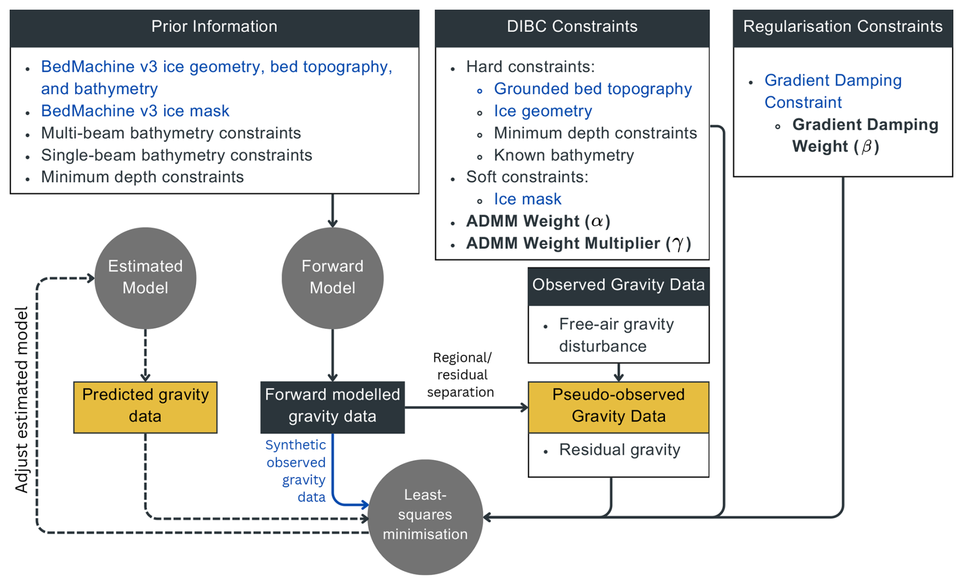
Figure 1 Schematic overview of the workflow used in this study. Dashed lines denote iterative processes completed during the inversion process. Orange elements denote gravity fields for which the misfit is minimised through the inversion process for the Vincennes Bay model. Bold text highlights key model parameters optimised through ensemble modelling. Blue text denotes components of the process used within the Synthetic model application.

2.2 Tomofast-x geophysical inversion platform

Tomofast-x is an open-source inversion platform capable of completing single and joint inversions using gravity and magnetic data (Giraud et al., 2021; Ogarko et al., 2021, 2024). Tomofast-x has previously been applied to various geophysical investigations (e.g. Martin et al., 2025; Giraud et al., 2023; Martin et al., 2021; Ogarko et al., 2021; Giraud et al., 2019). Working to minimise a least-squares cost function, Tomofast-x allows various geophysical, geological, and petrophysical data to be integrated into a constrained inversion model that includes a priori knowledge. The general application of Tomofast-x used here is shown in Fig. 1.

Tomofast-x models can be constrained by various techniques, in combination, including total variation (TV)-like regularisation to smooth the model (“gradient damping” constraints; Giraud et al., 2021; Li and Oldenburg, 1996; Rudin et al., 1992) as well as disjoint interval bound constraints (DIBCs; Ogarko et al., 2021) that provide physical bounds on model properties. Gradient damping aims to minimise the spatial variation of properties between neighbouring cells, reducing noise and complexity within the model (Li and Oldenburg, 1996). DIBCs specify the number of possible lithologies for a given model cell and provide upper and lower bounds for acceptable properties within each lithology (Ogarko et al., 2021). In Tomofast-x, DIBCs are enforced using the alternating direction method of multipliers (ADMM; Ogarko et al., 2021). Tomofast-x supports a non-uniform rectangular grid, allowing flexible model resolution and arbitrary surface topography to be included (Ogarko et al., 2024). The flexible mesh definition allows the use of decreased vertical resolution at depth (i.e. increasing vertical thickness) and decreased horizontal resolution around the model boundary to improve computational efficiency. Furthermore, the use of wavelet compression reduces memory requirements and further increases computational efficiency, without significant loss of resolution (Ogarko et al., 2024). Tomofast-x applies a property inversion (i.e. adjustment of individual cell properties) to solve inverse problems. However, the inclusion of DIBCs allows geometry-like inversions by separating the model into multiple lithologies, providing a versatile tool for geophysical applications across Antarctica.

For further details on the complete technical and numerical capabilities of Tomofast-x, we refer the reader to Giraud et al. (2021, 2023) and Ogarko et al. (2021, 2024). Key components of the inversion framework that are used in this study are further described below and shown in Fig. 1.

We use DIBCs to geometrically constrain regions of our models based on a priori information (Figs. 1 and 2). We include three unique lithologies (ice, water, and rock) within our models and use a priori information to discretise and assign properties to our model mesh (Fig. 2). Hard bound constraints are used to enforce geometric constraints, essentially forcing the model geometry to be “fixed” in specified regions (e.g. across regions of grounded ice, floating ice geometry, and in regions of known bathymetry). Soft bound constraints designate possible lithologies for each model cell in regions where geometry is allowed to vary (e.g. below floating ice and across open ocean). Details on the specific use of hard and soft bound constraints for this study are provided in Sect. 3.4.

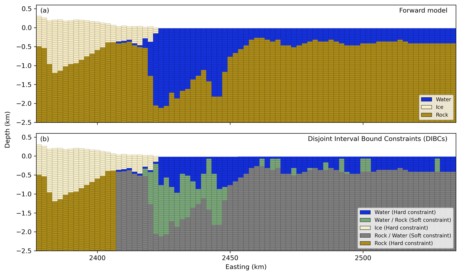
Figure 2 Example cross-section of the Vincennes Bay forward model and example DIBCs along northing = −897 km. (a) Discretisation of model cells used in the Vincennes Bay forward model. (b) Example usage of DIBCs along the same cross-section showing soft bound constraints used to enforce the ice mask and hard bound constraints to fix bed topography on grounded ice, ice geometry, minimum depth constraints in regions where seal dive data exist and to ensure floating ice remains floating.

We use gradient damping constraints to “smooth” the model, minimising non-physical features arising from the ill-posed nature of gravity inversions. For each model, the relative influence of DIBCs and gradient damping constraints on the overall cost function must be appropriately selected to ensure a physically plausible inversion result. The relative influence of each constraint type is controlled by weighting parameters, where the ADMM weight (α; Fig. 1) controls the DIBCs contribution, and the gradient damping weight (β; Fig. 1) controls the contribution from gradient damping. Here, we use ensemble modelling to quantitatively select optimal parameters based on physical model success criteria (Sect. 4.1).

3 Data and methods

3.1 Vincennes Bay study area

Vincennes Bay is a region with the warmest intrusions of mCDW and the fastest retreating glacier in East Antarctica (Picton et al., 2023; Ribeiro et al., 2021), where a deep marine canyon (the “Vanderford Valley”) was mapped offshore the Vanderford Glacier (Commonwealth of Australia, 2022, Fig. 3b). The Vanderford Glacier grounding line retreated over 18 km between 1996 and 2020 (Picton et al., 2023). Other smaller outlet glaciers (Adams, Anzac, Bond, and Underwood) neighbour Vanderford Glacier to the west (Fig. 3a) and have also experienced grounding line retreat in recent decades (Picton et al., 2023). High sub-ice-shelf basal melting is believed to drive grounding line retreat at Vanderford Glacier (Bird et al., 2025), with the Vanderford Valley likely providing a pathway for mCDW into the Vanderford Glacier ice shelf cavity. However, the pathway for warm water from the continental shelf to the Vanderford Valley and into the ice shelf cavity remains unknown. Containing approximately 0.67 m of global sea level rise equivalent (Morlighem et al., 2020), the Vincennes Bay drainage basin contributes to the larger Aurora Subglacial basin, which contains 7 m of global sea level rise equivalent and predominantly loses mass via the Totten Glacier. The close relationship between Totten Glacier and Vanderford Glacier (McCormack et al., 2024) highlights the importance of improving understanding of the Vanderford Glacier.

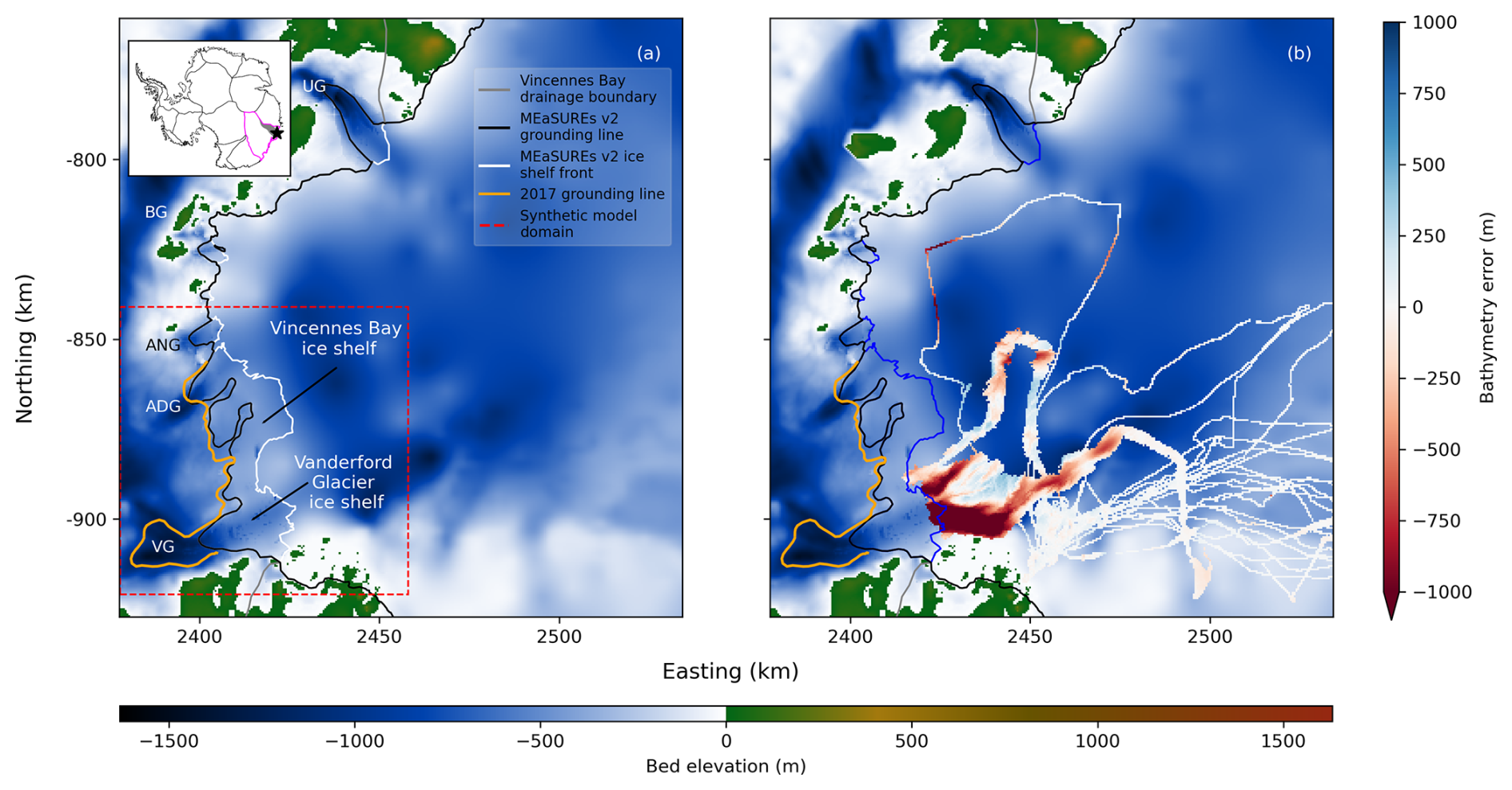
Figure 3 Overview of Vincennes Bay study area. (a) BedMachine v3 bed topography and bathymetry (IBCSO v2) (Morlighem et al., 2020). The black line denotes the MEaSUREs v2 grounding line from Mouginot et al. (2017). The Vincennes Bay drainage boundary is shown in grey. The 2017 grounding line is shown in orange (Picton et al., 2023). The red dashed line denotes the extent of the model core for the Synthetic model. Abbreviations are as follows: VG = Vanderford Glacier; ADG = Adams Glacier; ANG = Anzac Glacier; BG = Bond Glacier; UG = Underwood Glacier. The Vanderford Glacier ice shelf is not explicitly defined by Mouginot et al. (2017), but here we use “Vanderford Glacier ice shelf” to refer to the portion of the Vincennes Bay ice shelf that includes the main trunk of the Vanderford Glacier. The inset in (a) shows the extent of the Aurora Subglacial Basin (magenta outline) and the location of Vincennes Bay (black star). (b) All components consistent with (a), overlain with the bathymetry difference between IBCSO v2 bathymetry (i.e. from BedMachine v3; Morlighem et al., 2020) and mapped multibeam (Commonwealth of Australia, 2022) and single beam (Walter et al., 2016; Vander Reyden et al., 2016; Sowter et al., 2016) bathymetry. The extent shown in (a) and (b) denotes the area of interest and model core for the Vincennes Bay model.

Bathymetric mapping across Vincennes Bay has previously been limited, and the recent multibeam mapping (Commonwealth of Australia, 2022) revealed differences of up to 1890 m between the newly mapped regions and existing bathymetry estimates (Fig. 3b). Historic single beam acoustic depth soundings (Sowter et al., 2016; Vander Reyden et al., 2016; Walter et al., 2016) highlight regions offshore Adams Glacier with differences in excess of 1200 m (Fig. 3b). Furthermore, depth measurements from instrumented seal dives identify locations where regional bathymetric estimates are too shallow (McMahon et al., 2023; Ribeiro et al., 2021), albeit with greater uncertainty than ship-based observations. These differences suggest that deep pathways for mCDW into sub-ice-shelf cavities have not been well represented in ocean models to date. Therefore, ocean models are likely to poorly represent warm water pathways into the ice shelf cavity and associated sub-ice-shelf basal melt rates at Vanderford Glacier. This highlights the need for improved bathymetry estimates in this vulnerable region, particularly resolving large-scale bathymetric features that impact ocean circulation and connect sub-ice-shelf cavities with warm water masses across the continental shelf.

3.2 Airborne gravity data

The International Collaborative Exploration of the Cryosphere through Airborne Profiling (ICECAP) programme has been collecting airborne geophysical data in Antarctica since 2008. For this study, we use data from the ICP8 campaign, collected in 2017 (Roberts et al., 2018). Additional data are available in the study area due to the close proximity of the Casey Station staging area; however, ICP8 flights provide the only targeted survey of Vincennes Bay. Most other data are high-elevation transit flights to/from other regions, lacking the fidelity of low-altitude dedicated survey flights. Data are published as free-air gravity disturbances, calculated from the GRS-80 gravity model and relative to the WGS-84 ellipsoid (Fig. 4d).

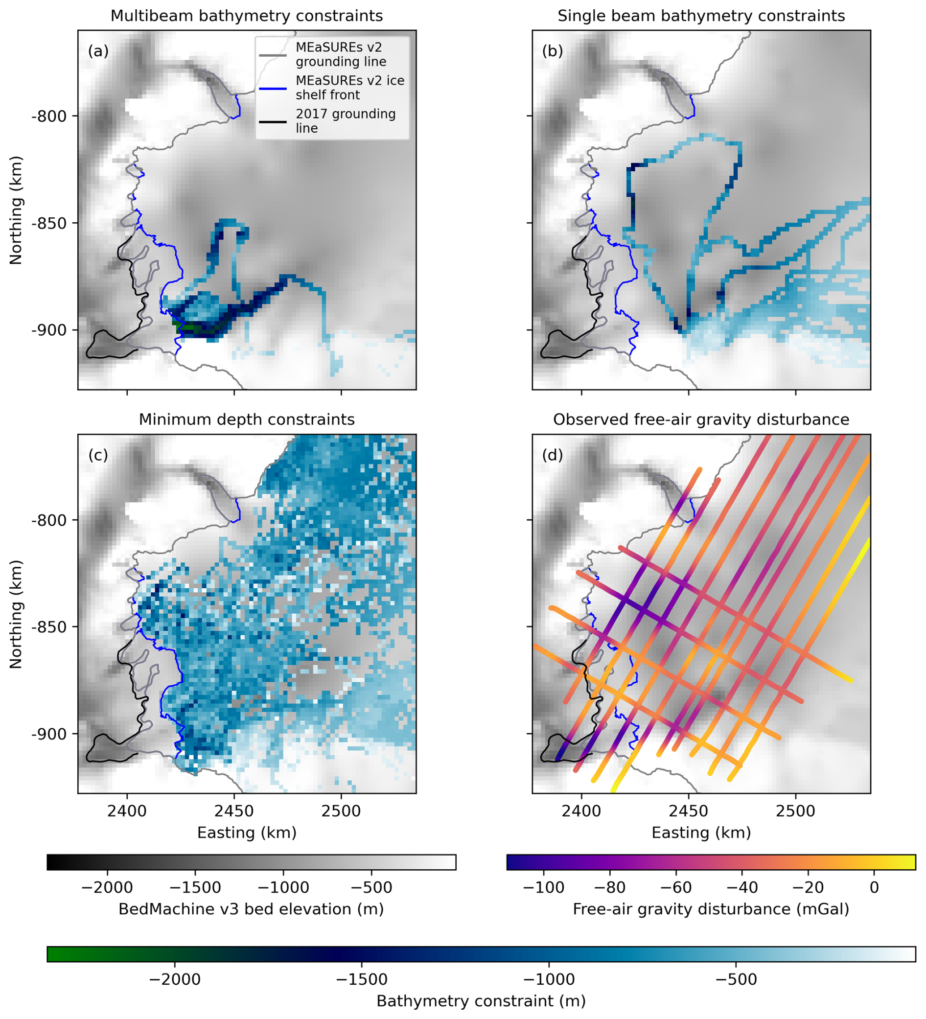
Figure 4 Known bathymetric constraints and observed free-air gravity data. (a) Multibeam bathymetry constraints (Commonwealth of Australia, 2022). (b) Single beam bathymetry constraints (Sowter et al., 2016; Vander Reyden et al., 2016; Walter et al., 2016). (c) Minimum depth constraints from instrumented seal dives (McMahon et al., 2023). (d) Observed free-air gravity disturbance data from selected ICP8 flight lines (Roberts et al., 2018). In all panels, the grey and blue lines represent the MEaSUREs v2 grounding line and ice shelf front, respectively (Mouginot et al., 2017). The black line is the 2017 grounding line from Picton et al. (2023).

We select flight lines from the ICP8 campaign to ensure consistent flight line orientation and spacing of ∼10 km in the north–south direction and ∼20 km in the east–west direction. Data were generally acquired from surveys flown at an altitude of 700–1000 m above the WGS-84 ellipsoid, at an average speed of ∼80 m s⁻¹. We split individual flight lines into multiple segments where more than 1 km of along-line data are missing. We remove all turns, transit flights, and line segments < 25 km, and trim flight lines around Casey Station where gravity measurements are affected by aircraft take-off and landing. Data are published with a 150 s temporal along-track filter applied (Roberts et al., 2018), resulting in a nominal along-line resolution of ∼6 km. We quantify the uncertainty associated with instrumentation errors based on cross-over analysis from selected ICECAP flight lines. Using a simple Bouguer slab correction based on a density contrast of 1643 kg m⁻³ between rock and water, the root mean square error (RMSE) crossover error of 2.61 mGal corresponds to a bathymetry error of ∼38 m. Additional processing (e.g. gridding) of airborne gravity data for the Vincennes Bay model is described in Sect. 5. The generation of synthetic gravity observations for the application of our Synthetic model is described in Sect. 4.

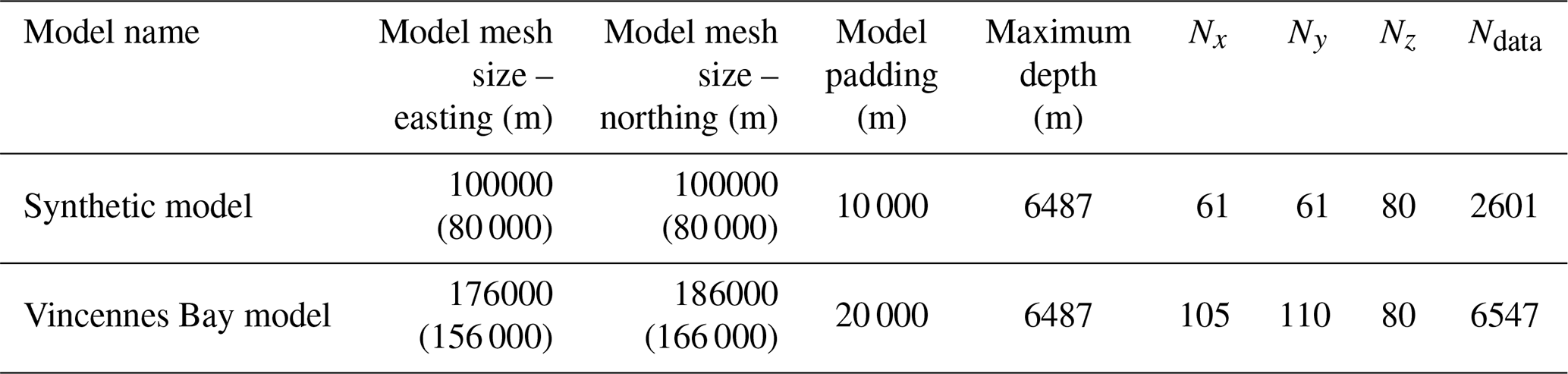
Table 1 Summary of model dimensions. Values in brackets represent dimensions of the model core (i.e. excluding the gravity buffer region from the model mesh). The model padding region extends beyond the model mesh in all directions.

3.3 Model setup and mesh

The Vincennes Bay model uses a terrain-following mesh at 2 km × 2 km horizontal resolution. The mesh comprises 80 horizontal layers and reaches a maximum depth of 6487 m. The vertical resolution is 50 m in the upper 3 km, increasing with depth by a factor of 1.1 below 3 km. To minimise edge effects from the boundary of the model or gravity data, which can introduce distortions or artefacts during the inversion procedure, we define a “model core” as the area of interest shown in Fig. 3 and generate a mesh that extends 10 km beyond (hereafter referred to as the “gravity buffer region”) the model core. We refer to the model core and gravity buffer region collectively as the “model mesh”. We provide observed gravity data across the model mesh. We then pad the model mesh (hereafter referred to as the “padding region”) using a horizontal resolution that coarsens by a factor of 1.1 from the edge of the buffer region (Table 1; Ogarko et al., 2024). Following the inversion, we remove the gravity buffer and padding regions before assessing the model. The Synthetic model is constructed in a consistent manner for a sub-region of the Vincennes Bay model (Fig. 3). Model mesh information is provided in Table 1.

3.4 Initial geometry and a priori information

We use existing bed topography, bathymetry, and ice geometry datasets from BedMachine v3 (Morlighem et al., 2020) to constrain our models using hard and soft bound constraints (Sect. 2.2). All data are referenced to the WGS-84 ellipsoid and interpolated onto a 2 km × 2 km mesh, consistent with the horizontal model resolution (Sect. 3.3), using bilinear interpolation. We discretise the model mesh using the BedMachine v3 ice mask (Morlighem et al., 2020) to identify regions of grounded ice, floating ice, ice-free land, and open ocean. However, we adjust the ice mask to correct the Vanderford Glacier grounding line position to the 2017 grounding line from Picton et al. (2023) to be consistent with the date of the gravity survey. This leads to an increase in the area of floating ice across the Vincennes Bay ice shelf (Fig. 3). Following interpolation to the model mesh and adjustment of the Vanderford Glacier grounding line, we re-impose the same geometric corrections used in BedMachine v3. That is, we assume all floating ice (including the new region of floating ice introduced at Vanderford Glacier) is in hydrostatic equilibrium and calculate the ice shelf thickness from the BedMachine v3 ice surface. Where the depth of the calculated ice base is lower than the BedMachine v3 sub-ice-shelf bathymetry (predominantly close to the grounding line) due to the effects of interpolation, we enforce a minimum water column thickness of 50 m by raising the ice base rather than lowering the bathymetry. Raising the ice base results in ice that is no longer in hydrostatic equilibrium; however, this approach prevents the introduction of unrealistic gradients in the initial bed topography close to the grounding line and is supported by the fact that the assumption of hydrostatic equilibrium is less robust close to the Vanderford Glacier grounding line (Chartrand and Howat, 2023).

For both the Synthetic and Vincennes Bay models, we initialise the models with grounded bed topography and the modified ice geometry discussed above and use hard bound constraints to fix regions of grounded ice and floating ice geometry. Soft bound constraints enforce the modified BedMachine v3 ice mask discussed above. This approach prevents floating ice from becoming grounded by enforcing a minimum water column of 50 m (i.e. one model cell) below floating ice. For the Vincennes Bay model, we make use of additional hard bound constraints in regions of known bathymetry from: (1) multibeam swath bathymetry mapping collected by the RSV Nuyina offshore the Vanderford Glacier (Commonwealth of Australia, 2022) and (2) single beam acoustic depth soundings collected during Australian Antarctic Division voyages since 2012 (Sowter et al., 2016; Vander Reyden et al., 2016; Walter et al., 2016). We interpolate multibeam swath bathymetry onto our model mesh using bilinear interpolation and take the median depth of single beam acoustic depth soundings within each 2 km × 2 km horizontal model cell. In addition, we use hard bound constraints to enforce minimum depth constraints across open-ocean regions using seal dive depths from McMahon et al. (2023). We select the deepest recorded dive depth within each 2 km × 2 km horizontal model cell. Where seal dives are deeper than mapped bathymetry, likely due to uncertainty in the estimated seal dive location (McMahon et al., 2023), we set the minimum depth constraint equal to the mapped bathymetry. A summary of bathymetric constraints used in the Vincennes Bay model is shown in Fig. 4. Additional information on the specific use of a priori information and hard and soft bound constraints for the Synthetic and Vincennes Bay models is provided in Sects. 4 and 5, respectively.

We assume homogeneous densities for ice (917 kg m⁻³), water (1027 kg m⁻³), and rock (2670 kg m⁻³). We model density contrasts, relative to the average crustal density of 2670 kg m⁻³, initialising our models with density contrasts of −1753, −1643, and 0 kg m⁻³ for ice, water, and rock, respectively.

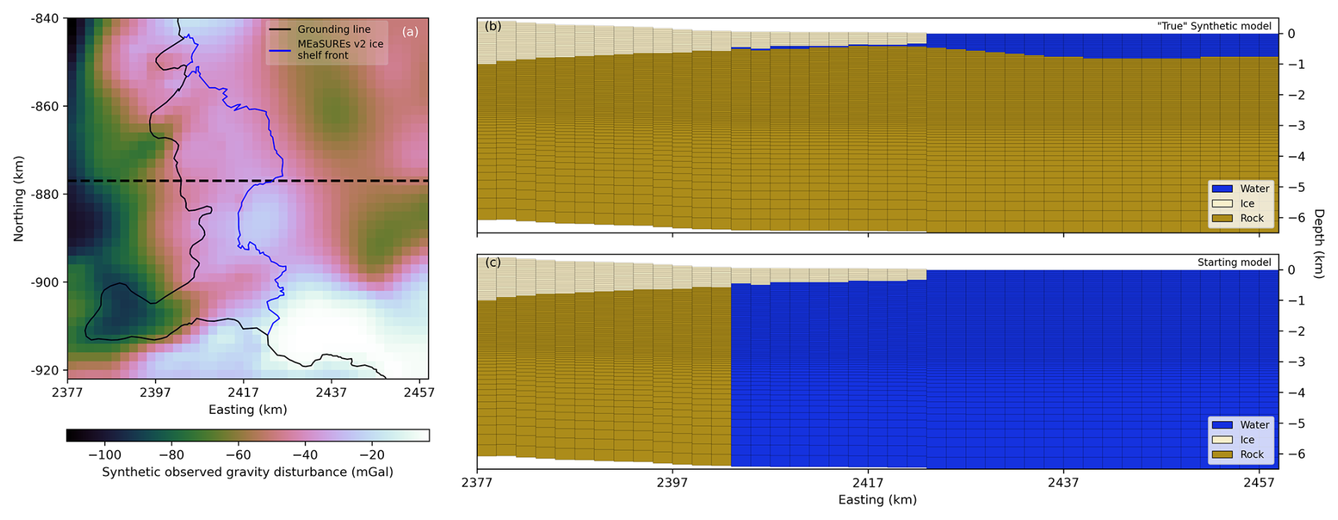
Figure 5 Overview of the Synthetic model. (a) Synthetic observed gravity data across the model core generated via forward modelling of the “True” Synthetic model. The black line denotes the MEaSUREs v2 grounding line, modified to include the 2017 grounding line from Picton et al. (2023). The blue line is the MEaSUREs v2 ice shelf extent. The black dashed line shows the cross-section along the centre of the model core (northing = −877 km) along which (b) and (c) are taken. (b) Example cross-section of the “True” Synthetic model. (c) Example cross-section of the starting Synthetic model.

4 Synthetic model application

The use of synthetic models reduces the ill-posed nature of the inversion problem since the “True” model is known. Therefore, they can be useful to understand the performance of an inversion algorithm for a particular use case. We use a realistic synthetic model to demonstrate the applicability of Tomofast-x to derive bathymetry from airborne gravity data and introduce a quantitative approach to model parameter selection. We construct a Synthetic model for a sub-region of the Vincennes Bay model domain (Fig. 3) using bed topography, ice geometry, and bathymetry from BedMachine v3 (Morlighem et al., 2020, Fig. 5b). We use hard bound constraints to constrain regions of grounded ice and ice geometry (Sect. 3.4) and do not include any hard bound constraints on bathymetry in regions of floating ice or open ocean. We forward model the gravity response of the Synthetic model to generate a synthetic gravity field (hereafter referred to as “synthetic observed gravity”) consistent with the “True” Synthetic model. We generate the synthetic observed gravity across the model mesh at a horizontal resolution of 2 km × 2 km (consistent with the horizontal model resolution) and a constant elevation of 1100 m to simulate an airborne gravity survey (Fig. 5a).

For the inversion, we initialise the model without an initial bathymetry so that the inversion is not influenced by any spurious initial geometries. That is, in regions of open water and below floating ice, we initialise the model as water throughout the entire depth of the model mesh (Fig. 5c). The padding region is initialised based on bed topography, ice geometry, and bathymetry from BedMachine v3 (Morlighem et al., 2020). We allow the inversion to continue for 300 iterations and use a wavelet compression rate of 0.1 to reduce memory usage and increase computational efficiency (Ogarko et al., 2024).

As mentioned in Sect. 2.2, the relative contribution of DIBCs and gradient damping constraints on the overall cost function must be carefully balanced to ensure physically plausible inversion results. Previous studies (e.g. Giraud et al., 2021; Martin et al., 2021) have used L-curve (Hansen and O'Leary, 1993) and L-surface (Bijani et al., 2017) analyses to identify optimal model parameters by selecting combinations that minimise the data misfit (i.e. the difference between simulated and observed data). However, L-curve and L-surface analyses do not evaluate the geological plausibility of a model. In the case of deriving bathymetry, relying solely on L-curve or L-surface analysis to select optimal parameter sets can lead to models that are not well defined (e.g. water can be introduced below rock without penalising the data misfit). Therefore, we consider the physical plausibility of a model by way of key “model success criteria”, including physical measures of model suitability (Sect. 4.1).

In Sect. 4.1, we introduce a quantitative ensemble modelling approach that aims to identify optimal model parameters by way of assessing “model success”. We apply this approach to the Synthetic model and discuss the results in Sect. 4.2.

4.1 Ensemble modelling approach

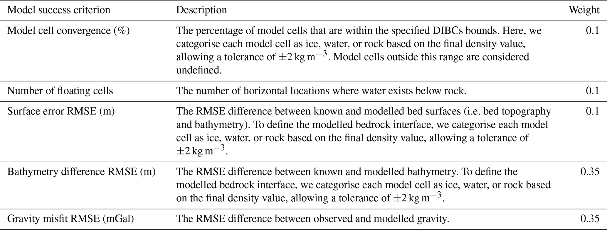
Table 2 presents five “model success criterion” which, when combined, provide a quantitative measure of overall model success. We examine the relative influence of different contributions from DIBCs (ADMM weight; α) and gradient damping constraints (gradient damping weight; β) on model success and identify optimal parameter combinations. We weight the model success criteria that assess the ability of the model to resolve accurate bathymetry while fitting the observed synthetic gravity data more heavily than other criteria in determining overall model success (Table 2). We note that the order of magnitude of each α and β parameter has a greater influence on model success than specific values; hence, we initially explore a range of parameters with different orders of magnitude. The ADMM weight can be dynamically adjusted during inversion by Tomofast-x using an additional user-defined parameter (i.e. ADMM weight multiplier, γ; Fig. 1) to subsequently fine-tune the α value once the appropriate order of magnitude is known. Accordingly, we perform a two-step ensemble approach where we first identify appropriate magnitude values of α and β and subsequently fine-tune the ADMM weight through a second ensemble that tests different γ values. For the initial ensemble, we test values of α and β (where γ=1 between $\mathrm{1}\times {\mathrm{10}}^{-\mathrm{9}}$ and $\mathrm{1}\times {\mathrm{10}}^{-\mathrm{2}}$) and also include a case with no gradient damping. This yields an ensemble of 72 Synthetic models, each with a unique parameter combination. Similar to the existence of multiple local optima within L-curve and L-surface analyses, this approach may identify multiple parameter sets that can yield comparable model results (Giraud et al., 2021; Bijani et al., 2017). Accordingly, we select models with comparable results to progress to the second ensemble stage.

Table 2 Model success criteria. Overall model success is calculated as the weighted sum of individual model success criteria using the weights specified. With the exception of model cell convergence, all model success criteria are calculated for the model core only. RMSE surface and bathymetry differences are calculated using a known bed surface derived from the forward model to ensure consistent biases from discretisation in the modelled and known bed surfaces.

For the second ensemble, we use the α and β values from the first ensemble and test different values of γ, to adjust the ADMM weight dynamically. We test γ values from 1.1 to 2, in increments of 0.1. We assess model success using consistent criterion weighting as the first ensemble (Table 2).

4.2 Results

Results of the initial ensemble modelling to identify optimal α and β parameters for the Synthetic model are shown in Fig. 6. We normalise results from each model success criterion and compute an overall model success score using the weighted sum of all criteria (Table 2; Fig. 6f). Note that the colour bars in Fig. 6a–f are such that light and dark colours represent good and poor success for each criterion, respectively. Figure 6f shows that, as with the use of L-curve and L-surface analyses, multiple parameter sets appear to yield largely comparable model results. The use of multiple physical criteria allows for additional interrogation of models with similar overall success.

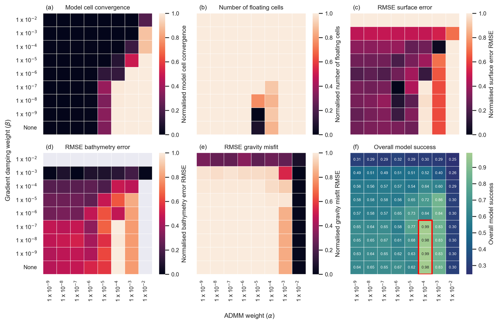
Figure 6 Normalised ensemble modelling results from the first Synthetic model ensemble. (a) Model cell convergence. (b) Number of horizontal locations where water exists below rock. (c) Surface difference RMSE. (d) Bathymetry difference RMSE. (e) Gravity misfit RMSE. (f) Overall model success calculated as the weighted sum of (a)–(e) using the weights specified in Table 2. The colour bars used in (a)–(f) show models with good success in light colours and models with poor success in dark colours. Grey cells in (d) indicate models for which a clear surface could not be determined. The red polygon in (f) denotes preferred models, all with comparable model success.

Figure 6 shows that for values of $\mathit{\alpha }>\mathrm{1}\times {\mathrm{10}}^{-\mathrm{4}}$, there is generally complete model cell convergence, unless high values of β (e.g. $>\mathrm{1}\times {\mathrm{10}}^{-\mathrm{4}}$) are used. However, for $\mathit{\alpha }>\mathrm{1}\times {\mathrm{10}}^{-\mathrm{4}}$, the estimated bedrock interface is consistently too deep (or unchanged from the starting model in the case of $\mathit{\alpha }=\mathrm{1}\times {\mathrm{10}}^{-\mathrm{2}}$) and the gravity misfit is consistently very high. This behaviour suggests $\mathit{\alpha }>\mathrm{1}\times {\mathrm{10}}^{-\mathrm{4}}$ is too high and DIBCs are satisfied too quickly, at the expense of the model appropriately fitting the synthetic observed gravity data. Models with α values < $\mathrm{1}\times {\mathrm{10}}^{-\mathrm{4}}$ show limited model cell convergence (Fig. 6a). Lower model cell convergence subsequently leads to higher bathymetry difference root mean square error (RMSE) values since the bedrock interface is less well defined (Fig. 6d). The influence of different magnitude α values on individual model success criterion (Fig. 6) suggests the optimal α value is between $\mathrm{1}\times {\mathrm{10}}^{-\mathrm{4}}$ and $\mathrm{1}\times {\mathrm{10}}^{-\mathrm{3}}$.

The influence of the magnitude of different β values is most apparent on model cell convergence (Fig. 6a), with higher β values generally leading to lower percentages of model cell convergence. Figure 6c and d shows that β values > $\mathrm{1}\times {\mathrm{10}}^{-\mathrm{4}}$ generally result in models with no clear bedrock interface at any location due to over-smoothing. The necessity of high model cell convergence to identify a clear bedrock interface suggests that β values ≤ $\mathrm{1}\times {\mathrm{10}}^{-\mathrm{7}}$ yield optimal model results. Figure 6f shows four models with similar overall model success scores (i.e. with α values of $\mathrm{1}\times {\mathrm{10}}^{-\mathrm{4}}$ and β values ≤ $\mathrm{1}\times {\mathrm{10}}^{-\mathrm{7}}$), which we refine in the second ensemble.

Each of the selected models includes some locations where water exists below rock (e.g. <0.5 % of horizontal points in the model core) and some do not quite reach complete model cell convergence (e.g. >99 %). To further improve the final model, we perform a secondary ensemble, testing different values of γ used to dynamically increase the ADMM weight as the inversion progresses. Here, we choose a data cost threshold of $\mathrm{1.4}\times {\mathrm{10}}^{-\mathrm{2}}$ such that α is increased by a given factor (γ) whenever the data cost reaches values below $\mathrm{1.4}\times {\mathrm{10}}^{-\mathrm{2}}$. We select the threshold of $\mathrm{1.4}\times {\mathrm{10}}^{-\mathrm{2}}$ so that the ADMM weight is adjusted after only a few iterations. When assessing model success from the second ensemble, we exclude models that do not reach 100 % model cell convergence. Figure 7 shows overall model success from the second ensemble modelling stage. Results for individual model success criteria are provided in Fig. S1 in the Supplement. The red star on Fig. 7 highlights the final selected model, with the highest overall model success. Note that all models in this second ensemble stage still have a few occurrences of water cells below rock. Accordingly, we correct these non-physical artefacts within the model core (by recategorising water cells below rock as rock) and run one additional forward simulation to generate a final model. We note that correcting these artefacts does not affect the modelled bathymetry, and the gravity misfit RMSE is changed by <1 %, highlighting that the presence of these artefacts is unlikely to have biased our model selection process or the final modelled bathymetry. The final modelled bathymetry is shown in Fig. 8b and has an RMSE error of 28 m compared to the “True” model (Fig. 8a) and an RMSE gravity misfit of 0.76 mGal (<1 % of the dynamic range of synthetic observed gravity data). Figure 8 shows that Tomofast-x is able to derive sub-ice-shelf and open-ocean bathymetry comparable to the Synthetic model, with only localised errors that are highest close to the grounding line where the model transitions between hard and soft bound constraints.

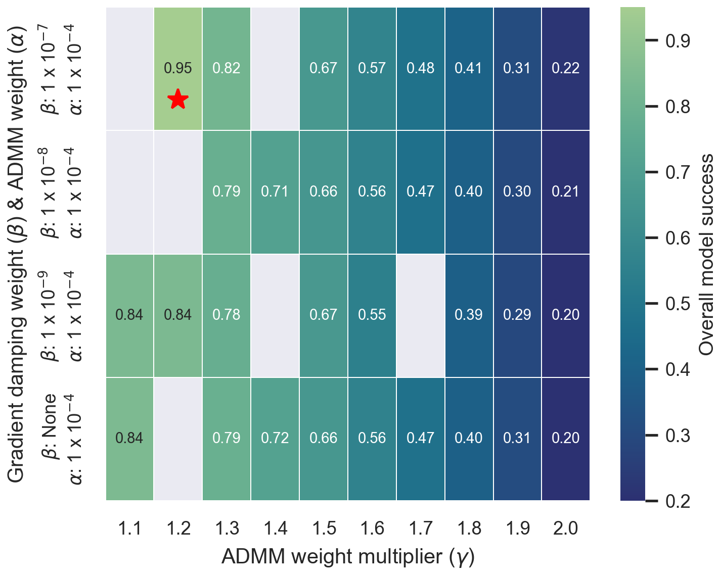
Figure 7 Overall model success from the second stage ensemble modelling. The red star indicates the final selected model. Grey cells indicate excluded models that did not reach 100 % cell convergence.

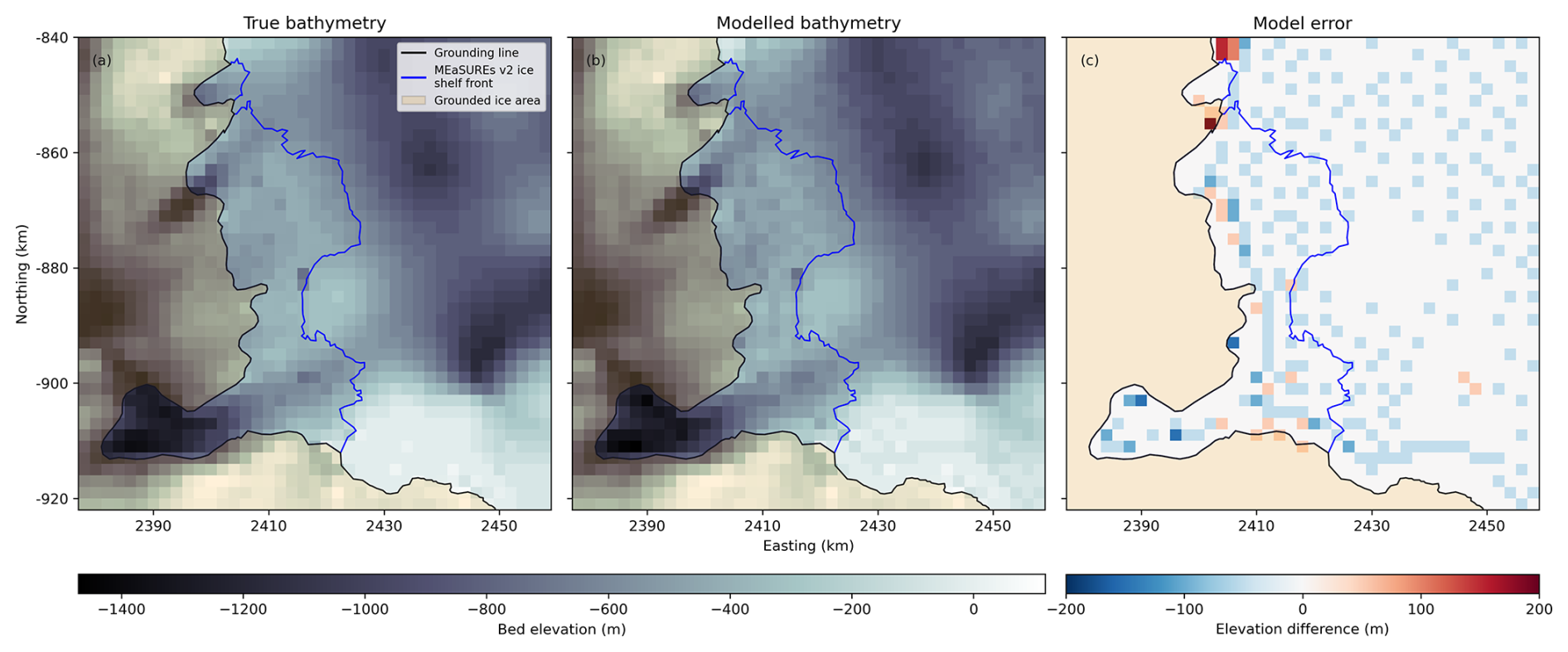
Figure 8 Final Synthetic modelled bathymetry. (a) “True” Synthetic model bed topography. (b) Modelled Synthetic bed topography. (c) Model error (b) − (a). Orange shading denotes grounded ice, and the black line is the MEaSUREs v2 grounding line, modified to include the 2017 grounding line from Picton et al. (2023). The blue line is the MEaSUREs v2 ice shelf extent (Mouginot et al., 2017).

5 Vincennes Bay model

In this section, we present an improved bathymetry for the Vincennes Bay region in East Antarctica (Fig. 3). We describe specific details of airborne gravity data processing in Sect. 5.1 and present the results and discuss model uncertainty in Sect. 5.2.

Similar to the Synthetic model application, we run an ensemble of models with different α, β, and γ values to determine optimal parameter combinations. To reduce the ensemble size, we select a subset of α and β parameter combinations, excluding those that consistently returned poor model convergence for the Synthetic model application (Figs. S2 and S3). For the second stage of the ensemble modelling, we use a data cost threshold of $\mathrm{2.2}\times {\mathrm{10}}^{-\mathrm{2}}$. During the ensemble modelling, we do not include hard bound constraints across regions of open ocean and below floating ice; rather, we use regions of mapped bathymetry to calculate the bathymetry RMSE, which is used to assess model success (Table 2). All other components of the model initialisation are consistent with the Synthetic model, as described in Sect. 4.

5.1 Forward model and airborne gravity data processing

We grid airborne gravity data (Sect. 3.2) at 2 km × 2 km horizontal resolution across the model mesh (consistent with the horizontal model mesh resolution; Sect. 3.3), using the equivalent source technique (Soler and Uieda, 2021) and continue the data upward to a constant elevation of 1100 m. To select optimal parameters required for the equivalent source model (i.e. relative source depth and damping parameters), we use a cross-validation technique (Soler and Uieda, 2021), identifying parameter combinations that yield the highest R² value between observed and modelled gravity values at observation locations. We select a relative source depth of 5 km and damping value of $\mathrm{1}\times {\mathrm{10}}^{-\mathrm{5}}$. Since regions of grounded ice are fixed using hard bound constraints, we mask the gravity data to regions allowed to vary during the inversion (i.e. regions of floating ice and open ocean) and 10 km upstream of the grounding line. Gridded gravity observations are shown in Fig. 9a.

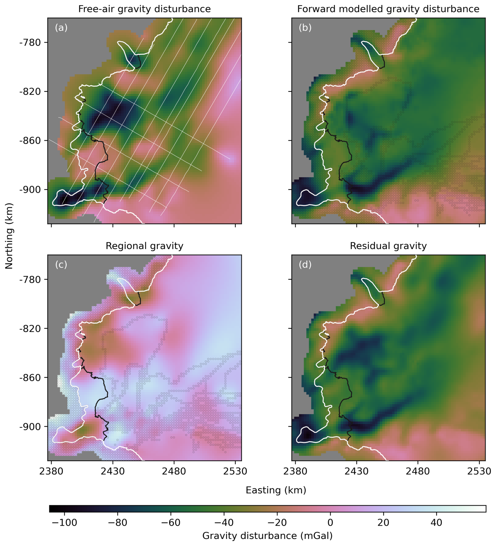
Figure 9 Processing of airborne gravity data. (a) Free-air gravity disturbance. (b) Forward modelled gravity disturbance from the Integrated IBCSO bathymetry. (c) “Regional gravity” derived from interpolated gravity misfit. (d) Residual gravity used as input to gravity inversions. The thick white line denotes the MEaSUREs v2 grounding line, modified to include the 2017 grounding line from Picton et al. (2023). The black line is the MEaSUREs v2 ice front. Thin white lines in (a) show select flight line locations. Black-outlined points in (b) and (c) identify points of known geometry used to interpolate the gravity misfit across the domain.

We construct a forward model for the Vincennes Bay model using bed topography and ice geometry from BedMachine v3 and merge available bathymetry mapping (Fig. 4a and b) and minimum depth constraints from instrumented seal dives (McMahon et al., 2023, Fig. 4c) with the existing IBCSO v2 (from BedMachine v3) bathymetry estimate. That is, in regions where instrumented seal dives are deeper than IBCSO v2, we set the bathymetry equal to the seal dive depth and use bilinear interpolation across a distance of 2 km around the boundary of each adjusted region to prevent sharp gradients in the adjusted bathymetry. We then integrate mapped bathymetry (Sect. 3.4) using the same bilinear interpolation technique to prevent sharp gradients around the boundary of the mapped bathymetry. We refer to this integrated bathymetry as the “Integrated IBCSO bathymetry” hereafter and forward model the gravity response to this initial bathymetry (Fig. 9b).

We perform regional/residual separation using an approach that leverages gravity misfits at locations of known geometry (An et al., 2019). We compute the gravity misfit between observed and forward modelled gravity at all locations where the geometry is known (i.e. “constraint points”; regions of grounded ice and mapped bathymetry). Gravity misfits at these locations are then interpolated across the whole domain using minimum curvature interpolation (Uieda, 2018, Fig. 9c) to derive a “regional gravity” field. This “regional gravity” field provides an estimate of long-wavelength gravity contributions as well as local density variations in the shallow subsurface. We remove the “regional gravity” field from the observed gravity field to provide a residual gravity field that is used as input to our gravity inversions (Fig. 9d).

5.2 Results

The inversion model selected from the ensemble modelling yields the bathymetry shown in Fig. 10b, with an RMSE gravity misfit of 1.27 mGal (Fig. 10d). Ensemble modelling results for the Vincennes Bay model are shown in Figs. S2 and S3, identifying two models with comparable overall success (Fig. S3). We select the model that results in the smallest mean bathymetry error in regions of mapped bathymetry. As with the Synthetic model, the selected model has a few occurrences of water cells below rock, primarily close to the grounding line. These regions are associated with highly variable gravity residuals close to the grounding line, particularly in the eastern portion of our domain. We attribute the variable gravity residuals and unphysical occurrences of water below rock in these regions to the transition from hard bound constraints across grounded ice to soft bound constraints across open ocean. We discuss this limitation further in Sect. 6. We correct these unphysical artefacts in the model core (by recategorising water cells below rock as rock) and run one additional forward simulation to generate a final model, which has a subsequent RMSE gravity misfit of 1.84 mGal (<2 % of the dynamic range of the gravity data). We note that this post-processing does not affect the modelled bathymetry. Furthermore, the impact of these artefacts is localised to close to the grounding line in regions of coastline where no ice shelves are present and there is relatively little ice loss. Therefore, any impact on our modelled gravity (hereafter referred to as “gravity-derived bathymetry”) likely does not have considerable impact on subsequent sub-ice-shelf basal melt rates or ocean circulation (Sect. 6.2).

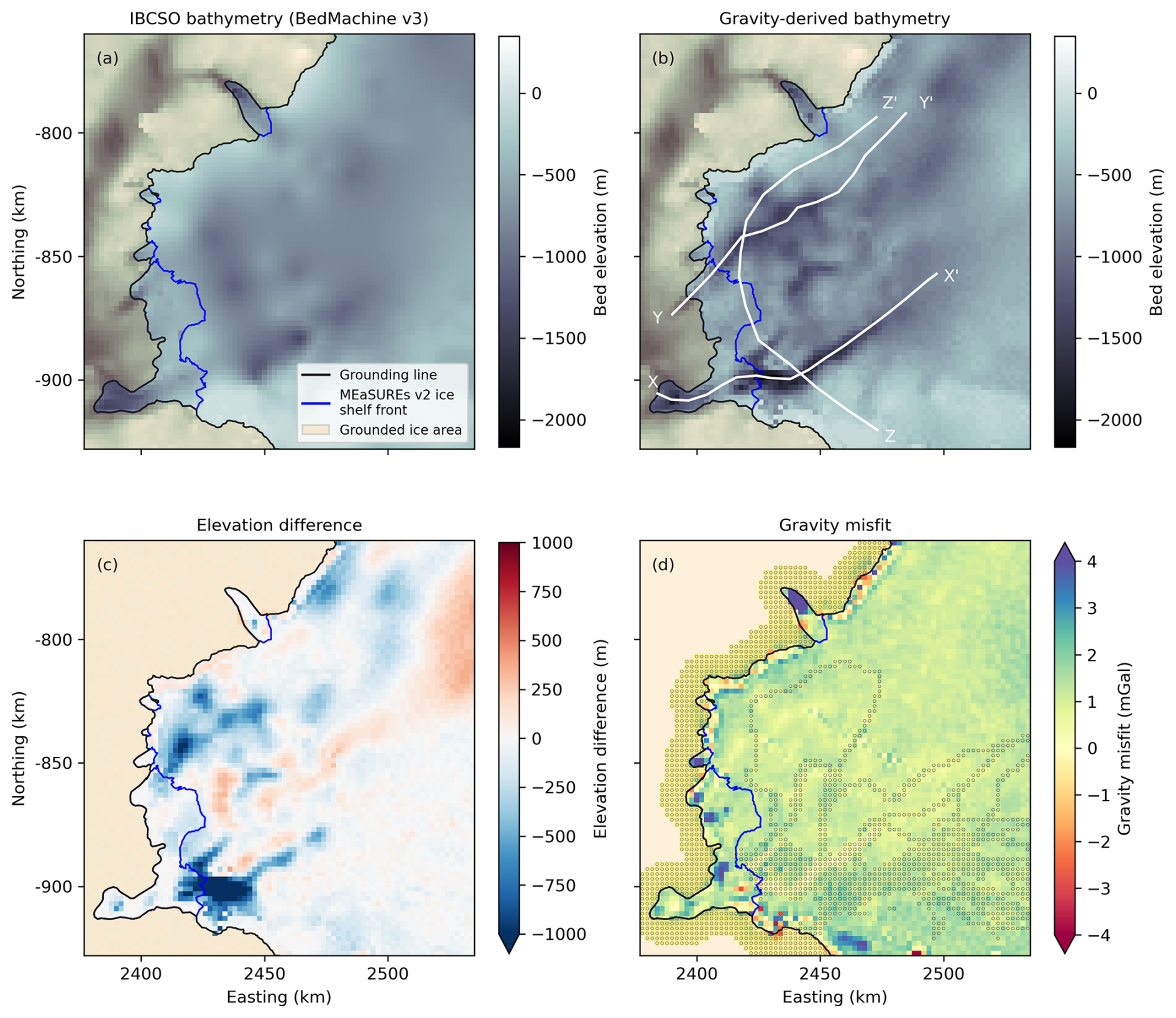
Figure 10 Vincennes Bay bathymetry derived from ensemble modelling. (a) IBCSO v2 (BedMachine v3) bathymetry. (b) Modelled bathymetry from gravity inversion (“gravity-derived” bathymetry). (c) Elevation difference calculated as (b) − (a). (d) Gravity misfit from gravity-derived bathymetry. Black outlined points in (d) identify points of known geometry used to interpolate the gravity misfit across the domain. Orange shading denotes grounded ice, and the black line is the MEaSUREs v2 grounding line, modified to include the 2017 grounding line from Picton et al. (2023). The blue line is the MEaSUREs v2 ice front. Profiles X–X', Y–Y', and Z–Z' on (b) are shown in Fig. 11.

5.2.1 Gravity-derived Vincennes Bay bathymetry

The gravity-derived bathymetry is, on average, 80 m deeper than IBCSO v2, with localised differences greater than 1850 m in the region of the Vanderford Valley (Fig. 10c). Our analysis reveals various large-scale bathymetric features that were not present in previous bathymetry estimates, with sub-ice-shelf and offshore bathymetry ranging from −63 to −2167 m (Fig. 10b). In particular, the gravity-derived bathymetry resolves the Vanderford Valley, a ∼6 km wide trough that extends ∼66 km offshore the Vanderford Glacier ice shelf cavity, reaching a maximum depth of 2167 m and connecting the Vanderford Glacier ice shelf cavity to the continental shelf (Figs. 10b and 11a). Towards the centre of the Vanderford Glacier ice shelf, gravity-derived bathymetry reveals a topographic sill that reaches an elevation of −556 m, upstream of which, and close to the present-day grounding line, the bathymetry deepens to ∼1600 m which is approximately 340 m deeper than IBCSO v2 (Figs. 10c and 11a). West of the Vanderford Valley, a smaller bathymetric trough, with an average depth of ∼1200 m, is revealed offshore the Adams Glacier (Fig. 11b and c). This feature extends ∼60 km offshore the Adams Glacier ice shelf cavity and reaches a maximum depth of 1566 m (Fig. 11b). Localised regions of high gravity misfit below floating ice (Fig. 10d) suggest potential grounding zones, where modelled water column thicknesses are <100 m (Fig. S4). In particular, below the Vincennes Bay ice shelf, regions of high gravity misfit and shallow water column correspond with localised regions of previously grounded ice based on the MEaSUREs v2 grounding line (Fig. S4). We note that by imposing a minimum water column thickness of 50 m (i.e. one vertical model cell) to enforce the modified ice mask (Sect. 3.4), our model does not explicitly allow grounding in these regions; however, it identifies regions where a shallow water column thickness may promote re-grounding of floating ice.

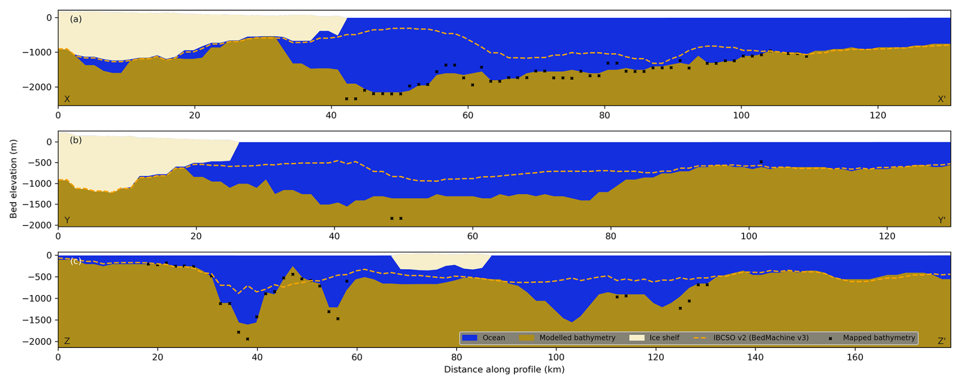
Figure 11 Two-dimensional cross sections of gravity-derived bathymetry along profiles shown in Fig. 10b. (a) Cross-section of gravity-derived bathymetry along profile X–X'. (b) Cross-section of gravity-derived bathymetry along profile Y–Y'. (c) Cross-section of gravity-derived bathymetry along profile Z–Z'. Solid brown areas show the gravity-derived bathymetry. Cream areas show Vincennes Bay ice shelves. Blue areas show regions of water. The dashed orange line shows the IBCSO v2 bathymetry estimate. Black crosses denote mapped bathymetry from single beam and multibeam bathymetry.

5.2.2 Model uncertainty

Quantifying errors in gravity inversions is challenging due to the combination of inherent uncertainties of the subsurface geology and associated assumptions and observational errors (some of which are discussed in more detail in Sect. 2). Here, we assess the uncertainty in our final bathymetry model (Fig. 10b).

Uncertainty associated with instrumentation errors results in a bathymetry error of ∼38 m (Sect. 3.2). We estimate the uncertainty associated with local variations in the geology that are not removed by the regional/residual separation (Sect. 5.1) using the gravity misfit at points of known geometry (i.e. grounded ice and mapped bathymetry). The RMSE gravity misfit of 1.0 mGal at constraint points corresponds to a bathymetry error of ∼15 m. The vertical resolution of the model grid (50 m) results in an inherent uncertainty of ±25 m due to the discretisation of all geometry data onto individual model cells. Without knowing the degree of correlation associated with individual components of model uncertainty, we sum individual sources of uncertainty (i.e. instrument uncertainty, geological uncertainty, and vertical model resolution) to provide a conservative uncertainty estimate of ±78 m.

Without using hard bound constraints to enforce minimum depth constraints from instrumented seal dives and mapped bathymetry during the ensemble modelling process, the geometry of open-ocean and sub-ice-shelf bathymetry is unconstrained. This provides an alternate approach to quantify model uncertainty, by comparing the gravity-derived bathymetry with mapped bathymetry. Figure 12 compares gravity-derived bathymetry with mapped bathymetry (Fig. 12a) and minimum depth constraints from instrumented seals (Fig. 12b). The gravity-derived bathymetry has a RMSE difference of 86 m (and a bias of −16 m) compared to mapped bathymetry (Fig. 12a). These uncertainty estimates are comparable with uncertainty estimates provided for other studies that derive bathymetry by way of gravity inversion (e.g. Eisermann et al., 2024; Constantino and Tinto, 2023; Jordan et al., 2020).

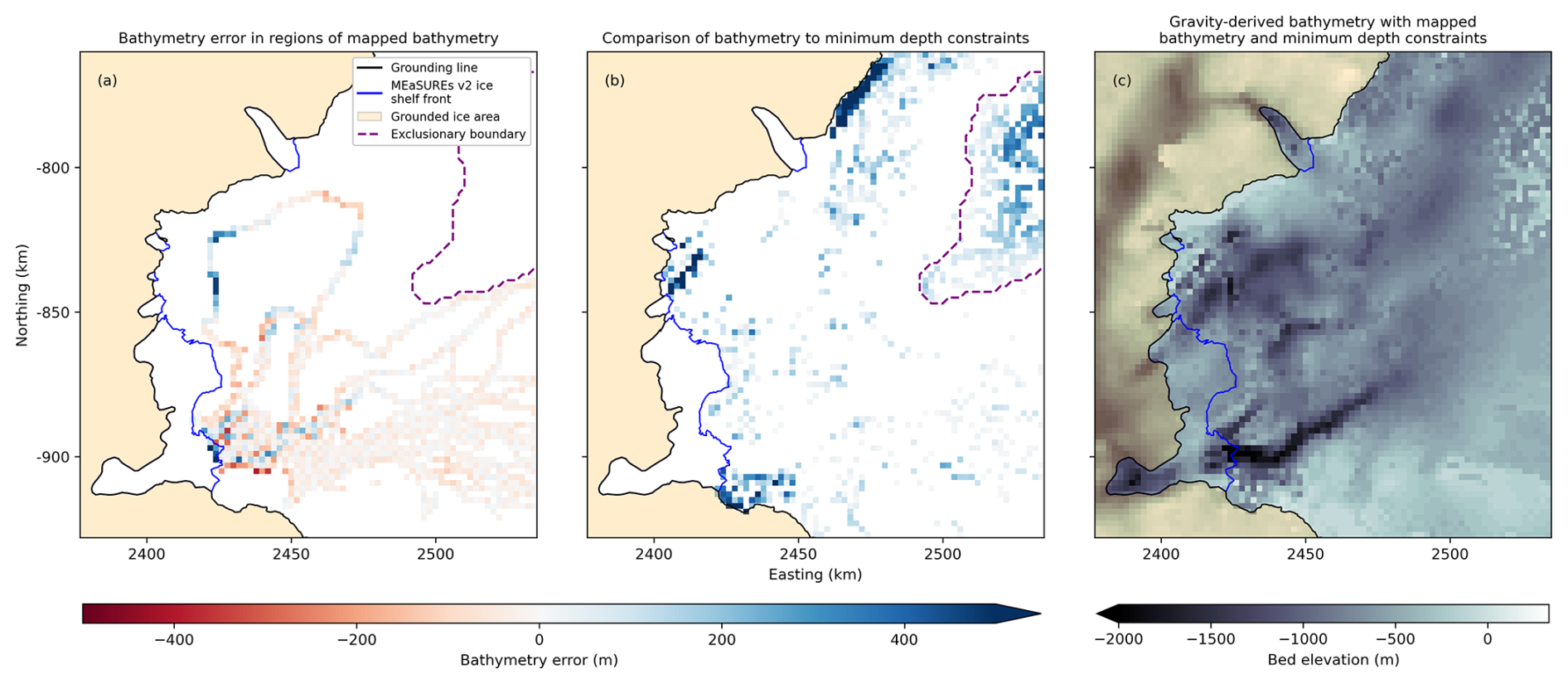
Figure 12 Gravity-derived bathymetry error. (a) Gravity-derived bathymetry error in regions of mapped bathymetry. (b) Comparison of gravity-derived bathymetry to minimum depth constraints. Blue regions denote areas where minimum depth constraints are deeper than gravity-derived bathymetry. (c) Gravity-derived bathymetry including mapped bathymetry and minimum depth constraints. The purple contour on (a) and (b) denotes the exclusionary boundary used when blending gravity-derived bathymetry with larger regional bathymetry.

Single beam bathymetry offshore Adams Glacier highlights a region where the gravity-derived bathymetry is up to 470 m too shallow (Fig. 12a). We attribute this to the method used to generate the Integrated IBCSO bathymetry applied in our forward model. That is, the narrow nature of single beam bathymetry estimates and the use of a 2 km interpolation distance to blend bathymetry datasets result in a narrow, deep bathymetric feature in this region that cannot be well resolved by the gravity inversion but is also likely not realistic. The smoother bathymetry returned by the inversion is likely more realistic, even if the absolute depth is not correct. Instrumented seal dives highlight a second region offshore, west of Underwood Glacier, where gravity-derived bathymetry is too shallow (Fig. 12b). We attribute this discrepancy to the scarcity of offshore bathymetry constraints, which has a direct impact on the accuracy of the regional/residual separation in this region. That is, the “regional gravity” field used in the regional/residual separation relies exclusively on interpolated values from far-field constraint points in this region, limiting the accuracy of, particularly, local density variations captured in this process. Accordingly, the offshore gravity high (Fig. 9d) drives an increase in mass in this region. Due to the homogeneous bedrock density used here, mass is controlled exclusively by changes in topography, resulting in shallow bathymetry returned in this region. We further discuss these limitations in Sect. 6.3. The discrepancy between gravity-derived bathymetry and minimum depth constraints from instrumented seal dives indicates that bathymetry is poorly resolved in this region. As such, we exclude this region of bathymetry when blending the gravity-derived bathymetry with larger regional bathymetry datasets to support ocean modelling (Sect. 6.2), ensuring a smooth transition at the edge of our model domain.

To provide a modelled bathymetry that directly integrates mapped bathymetry and minimum depth constraints from instrumented seal dives, we complete one additional inversion, with a starting bathymetry that combines mapped bathymetry and instrumented seal dives with the gravity-derived bathymetry returned from the ensemble modelling. We include hard bound constraints across regions of mapped bathymetry and enforce minimum depth constraints from instrumented seal dives, allowing the inversion to continue for 300 iterations (Fig. 12c). The resultant bathymetry shows high-frequency variations, particularly in the offshore region west of Underwood Glacier where gravity-derived bathymetry was previously too shallow. The use of minimum depth constraints results in high-frequency depressions in the bathymetry where model properties are enforced using hard bound constraints and cannot be altered through inversion. High-frequency variations are likely not realistic and arise primarily from the discrete nature of individual seal dives.

In addition to the model uncertainty noted above, the model resolution is limited by the resolvable wavelength of the gravity data. As noted in Sect. 3.2, the resolvable wavelength of gravity data used here is ∼6 km. Therefore, only bathymetric features with a wavelength ≥ 6 km are well resolved in our bathymetry model and significantly higher errors may occur in regions of rough bathymetry.

5.3 Vincennes Bay ocean modelling

Bathymetry is known to have important controls on sub-ice-shelf basal melt rates and ocean circulation (Goldberg et al., 2020). Given the common reliance of sub-ice-shelf basal melt estimates and/or basal melt parameterisations on regional ocean models, accurate regional bathymetry estimates are critical for reliably modelling nearshore ocean dynamics. Here, we apply a regional ocean model of Vincennes Bay using the Regional Ocean Modelling System (ROMS; Shchepetkin and McWilliams, 2005) to assess the impact that the potential warm water pathways revealed in our gravity-derived bathymetry have on sub-ice-shelf basal melting in Vincennes Bay. We run two model simulations, each with different ocean bathymetry: (1) using IBCSO v2 and (2) using our gravity-derived bathymetry. We compare the resultant modelled bottom ocean temperatures and sub-ice-shelf melt rates in Fig. 13.

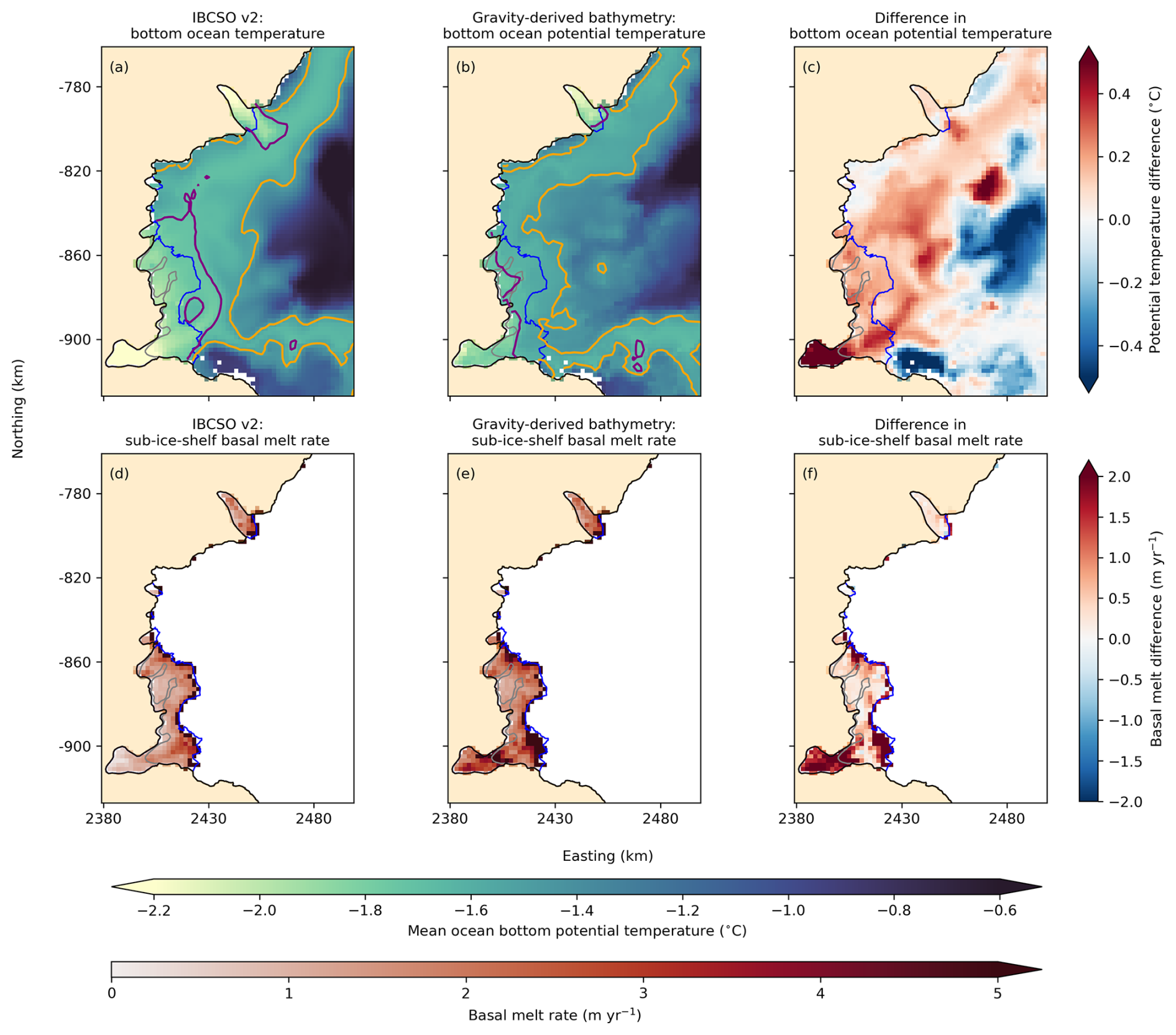
Figure 13 Mean annual modelled ocean bottom potential temperature and sub-ice-shelf basal melt rates for different bathymetry surfaces. (a) Modelled ocean bottom potential temperature using IBCSO v2 ocean bathymetry. (b) Modelled ocean bottom potential temperature using our gravity-derived bathymetry. (c) Difference in bottom ocean potential temperature, calculated as (b) − (a). (d) Modelled sub-ice-shelf basal melt rate generated using IBCSO v2 ocean bathymetry. (e) Modelled sub-ice-shelf basal melt rate generated using our gravity-derived bathymetry. (f) Difference in sub-ice-shelf basal melt rates, calculated as (e) − (d). Purple contours in (a) and (b) denote the lower bound of mCDW water temperatures (−1.7 °C) following Ribeiro et al. (2021). Orange contours in (a) and (b) denote water temperatures of −1.5 °C. Orange shading denotes grounded ice and the black line is the MEaSUREs v2 grounding line, modified to include the 2017 grounding line from Picton et al. (2023). The blue line is the MEaSUREs v2 ice shelf extent (Mouginot et al., 2017).

Ocean simulations were conducted with ROMS, with modifications for ice shelf mechanical pressure and thermodynamics, following Galton-Fenzi et al. (2012) and Dinniman et al. (2003). The model was built on a polar stereographic grid with a spatial resolution of ∼2 km and 25 vertical layers (producing minimum vertical resolutions of ∼10–20 m on the deep continental shelf and less than ∼2 m within the ice shelf cavity). This kernel has been previously employed for simulations of this region (e.g. Gwyther et al., 2014; McCormack et al., 2021). Lateral forcing (i.e. temperature, salinity, and velocity) is sourced from ACCESS-OM2-1 (Kiss et al., 2020). Surface forcing is also sourced from ACCESS-OM2-1 and consists of wind, heat, and salt fluxes, which together represent sea ice formation. We employ the sea ice flux parameterisation as used previously (e.g. Richter et al., 2022), rather than a dynamic sea ice model. Two simulations were conducted, where the only difference is the bathymetry surface product (i.e. IBCSO v2 and our modelled bathymetry). For further technical details on the model setup, we refer the reader to previous implementations of this model kernel (e.g. Gwyther et al., 2014).

High spatial gradients in ocean bathymetry can result in numerical instabilities in ocean models (Mellor et al., 1998), often requiring ocean modellers to “smooth” and/or manually adjust bathymetry datasets. As such, we use the gravity-derived bathymetry from the ensemble (Fig. 10b) without the high-frequency bathymetry variations introduced by integrating minimum depth constraints to minimise the amount of manual adjustment required for numerical stability. The bathymetry was smoothed to remove any overly steep gradients and a minimum water column (of ∼20 m) was enforced. The resulting change in bathymetry was minimal and key features (e.g. the Vanderford Valley and ice shelf cavity shape) were preserved. Ten years were simulated, with repeat annual forcing, and we analyse only the final year to allow a 9-year spin-up period.. We discuss the implications of warm water pathways revealed in our gravity-derived bathymetry on ocean circulation and basal melt rates in Sect. 6.2. We note that the limited scope of our ocean modelling is not intended to provide comprehensive estimates of sub-ice-shelf basal melt but to demonstrate the influence of different bathymetry estimates on basal melt rates.

6 Discussion

This study presents an open-source approach to deriving sub-ice-shelf and open-ocean bathymetry around Antarctica by way of geophysical inversion. Both the Synthetic and Vincennes Bay models demonstrate the applicability of Tomofast-x to derive accurate bathymetry through the use of DIBCs and an ensemble modelling approach.

6.1 Gravity-derived Vincennes Bay bathymetry using Tomofast-x

We integrate existing datasets of bed topography, mapped bathymetry, instrumented seal dives, and airborne gravity data to generate an improved bathymetry estimate for the Vincennes Bay region in East Antarctica. Our gravity-derived bathymetry highlights various bathymetric features that were previously unresolved in existing regional bathymetry estimates.

Our gravity-derived bathymetry identifies two large-scale bathymetric troughs that may provide pathways for warm water into the Vincennes Bay ice shelf cavity: the previously mapped Vanderford Valley and a smaller, previously unmapped trough into the Adams Glacier ice shelf cavity. These features are not dissimilar from an unknown trough recently identified through bathymetry mapping of the Totten Glacier. This trough enabled improved understanding of basal melt patterns within the ice shelf cavity and is expected to improve estimates of future sea level contributions from Totten Glacier (Vaňková et al., 2023). We explore the impact of the gravity-derived bathymetry on ocean dynamics and basal melt rates across Vincennes Bay in Sect. 6.2.

Our gravity-derived bathymetry also identifies a potential sill within the Vanderford Glacier ice shelf cavity (Figs. 10b and 11a) that likely plays an important role in the access of mCDW towards the Vanderford Glacier grounding line. Given the location of this topographic feature downstream of the 1996 grounding line location (i.e. MEaSUREs v2; Mouginot et al., 2017), it is possible that this feature was integral in grounding line persistence in previous decades and may have provided buttressing forces to the Vincennes Bay ice shelf (Fürst et al., 2016). However, the absence of geometry and/or density constraints within the Vanderford Glacier ice shelf cavity prevents confident determination of whether this feature is accurately modelled in the gravity inversion or arises as an artefact of our regional/residual separation methodology or assumed bedrock density (Sect. 6.3).

Comparison of our gravity-derived bathymetry to the recent pan-Antarctic gravity-derived bathymetry from Charrassin et al. (2025) (Fig. S5) highlights where high-resolution and regional studies can provide additional benefits in deriving bathymetry around Antarctica and indeed may be necessary for resolving some bathymetric features. Charrassin et al. (2025) use the Antarctic gravity anomaly and height anomaly grids (AntGG2021; Scheinert et al., 2024) that have a spatial resolution of 5 km. For Vincennes Bay, this has implications for how well the Vanderford Valley – a deeply incised, narrow channel that may be essential for the transport of warm water to the Vanderford cavity – is resolved. This also highlights the need for comprehensive swath bathymetry mapping across the continental shelf to reliably constrain gravity inversion models and the necessity for high-resolution airborne gravity to support local- and regional-scale gravity inversions for key areas around Antarctica, including within ice shelf cavities.

The bathymetry of Vincennes Bay has received little attention until recently, when depth measurements from instrumented seal dives identified regions of Vincennes Bay that were deeper than existing bathymetry estimates (McMahon et al., 2023; Ribeiro et al., 2021). There are uncertainties associated with data collected from instrumented seals; for example, McMahon et al. (2023) report a depth resolution of 25 m and use a 2.5 km horizontal resolution when analysing seal data to account for uncertainties in the seal dive location, while Padman et al. (2010) use a horizontal resolution of 2 km, consistent with the resolution used in this study. Furthermore, seals have rarely been recorded to dive to depths greater than ∼1200 m (Hindell et al., 2016), limiting the application of their dive depth data to regions of shallower bathymetry. Despite the uncertainties and limitations of these datasets, depth information collected by instrumented seals across vast regions around Antarctica provides valuable data to: (1) identify regions of the continental shelf where current bathymetry estimates may be too shallow and (2) integrate into updated bathymetry estimates, particularly to identify large-scale bathymetric features that may provide warm water pathways towards the periphery of the continent. We acknowledge that integrating minimum depth data from instrumented seals using hard bound constraints in our inversion results in likely unrealistic high-frequency variations in modelled bathymetry (Sect. 5.2.2), particularly offshore west of Underwood Glacier; however, this behaviour should not discount the usefulness of these datasets and is attributed to model limitations and assumptions made within this study, which we discuss further in Sect. 6.3.

While the use of airborne gravity data to derive sub-ice-shelf and open-ocean bathymetry around Antarctica is not a new concept (e.g. Constantino and Tinto, 2023; Eisermann et al., 2021; Yang et al., 2021; Constantino et al., 2020; Eisermann et al., 2020; Jordan et al., 2020; Tinto et al., 2015), the use of Tomofast-x provides a flexible and open-source approach to such an application. As discussed in Sect. 2.1, there are numerous approaches to both gravity data processing and geophysical inversions, each with their own advantages and limitations, and the choice of one is often dependent on available a priori information. The flexibility of Tomofast-x, coupled with ensemble modelling and the programmatic workflow developed for this study, allows the exploration of multiple approaches and the evaluation of the impact of models and assumptions of varying complexity in deriving improved bathymetry estimates around Antarctica. We discuss possible alternate approaches to refine and improve the assumptions of homogeneous density and regional/residual separation used here in Sect. 6.3.

6.2 Warm water pathways and implications for basal melt across Vincennes Bay

To assess the implications of warm water pathways revealed in our gravity-derived bathymetry on ocean bottom temperatures and sub-ice-shelf melt rates, we compare ocean model output from our two ocean model simulations (Sect. 5.3).

The gravity-derived bathymetry leads to increased nearshore bottom ocean temperatures across Vincennes Bay and localised increased temperatures in excess of 0.75 °C within the Vanderford Glacier ice shelf cavity (Fig. 13c). Given the classification of mCDW water masses from Ribeiro et al. (2021) (i.e. water masses with potential temperatures between −1.7 and 1.5 °C), our modelling suggests that no mCDW enters into the Vanderford Glacier ice shelf cavity when using the IBCSO v2 bathymetry (Fig. 13a), while our gravity-derived bathymetry allows mCDW access into the ice shelf cavity (Fig. 13b). Figure S6 shows a two-dimensional cross-section of ocean temperatures within and offshore the Vanderford Glacier ice shelf cavity, along northing −905 km, highlighting increased temperatures in the ice shelf cavity with our gravity-derived bathymetry. This finding is consistent with recent studies that suggest that sub-ice-shelf basal melt, driven by mCDW access to the ice shelf cavity, is likely responsible for rapid grounding line retreat at Vanderford Glacier (Bird et al., 2025; McCormack et al., 2023; Picton et al., 2023). Similarly, west of the Vanderford Glacier, the smaller bathymetric trough offshore the Adams Glacier (Fig. 11b) provides a pathway for mCDW to the Adams Glacier ice shelf cavity (Fig. 13b).

Figure 13d–f shows modelled sub-ice-shelf basal melt rates returned by our ocean model simulations. Sub-ice-shelf basal melt rates generated from our gravity-derived bathymetry are, on average, 37 % higher across all ice shelves within Vincennes Bay and 54 % higher across the Vincennes Bay ice shelf, compared to those modelled using IBCSO v2 bathymetry. Compared to those generated using the IBCSO v2 bathymetry, basal melt rates generated using our gravity-derived bathymetry are closer to current satellite-derived estimates (e.g. Paolo et al., 2022; Davison et al., 2023), suggesting that large-scale bathymetric features in the region likely have an important influence on sub-ice-shelf melting at Vanderford Glacier. Our modelling highlights localised differences of up to 6.6 m yr⁻¹ across the Vincennes Bay ice shelf (Fig. 13f), with large increases close to the grounding zone, where the glacier dynamics are most sensitive to changes. The discrepancy in mCDW access and basal melt rates across Vincennes Bay ice shelf cavities between the two model runs highlights the critical influence of bathymetry on our understanding of near-shore ocean circulation, basal melt rates, and subsequent ice sheet response.

6.3 Model limitations

The non-unique nature of gravity inversion often requires a number of simplifying assumptions that can limit the accuracy of inversion models. Here, we discuss particular assumptions and limitations within our methodology and the impact of those on our gravity-derived bathymetry.

Our regional/residual separation method (An et al., 2019; Millan et al., 2020) relies on known geometry at constraint points across the inversion domain. The spatial distribution of these constraint points impacts the accuracy of the interpolated “regional” gravity field and, subsequently, the inversion model, with errors increasing with distance from the constraint points (Millan et al., 2020). In poorly constrained regions, it is not possible to deduce the cause of observed gravity disturbances (i.e. whether they arise from changes in topography or density variations). For example, west of Underwood Glacier, an offshore gravity high in the observed gravity disturbance field (Fig. 9a) persists in the residual gravity field used as input to the inversion (Fig. 9d). However, the lack of geometry constraints in this region results in uncertainty in the origin of this gravity signal and increased uncertainty in the gravity-derived bathymetry in this region (Sect. 5.2.2). Furthermore, the choice of interpolation technique used to interpolate gravity misfits from constraint points can influence the resultant gravity field and thus the subsequent inferred bathymetry. Here, we interpolate gravity misfits using a minimum curvature algorithm to ensure that the calculated gravity misfits at constraint points are respected, since data at these locations provide the highest-confidence gravity data. Comparison of different interpolation methods on the resultant gravity-derived bathymetry was outside the scope of this study. To our knowledge, no studies have quantitatively assessed the optimal distribution of geometry constraints and the influence of different interpolation techniques to ensure reliable inversion results, and this should be a focus of future research efforts.

Our regional/residual separation relies on forward modelled gravity at constraint points. However, since local gravity disturbances are influenced from near- and far-field sources, surrounding topography can influence forward modelled gravity at constraint points. Therefore, uncertainty in topographic (i.e. BedMachine v3) and bathymetric constraints included in the forward model can influence the residual gravity field and propagate into the final inversion. Within our inversion domain, uncertainty estimates of bed topography in BedMachine v3 exceed 500 m in some inland regions (Morlighem et al., 2020) and a few hundred metres in some coastal regions close to the grounding line. Some previous studies complete two-dimensional gravity inversions along flight lines with coincident gravity and radar data to limit uncertainties associated with forward modelled bed topography (e.g. Constantino and Tinto, 2023). However, BedMachine v3 integrates all available airborne radar data for the Vincennes Bay region and provides the most up-to-date and publicly available estimate of bed topography suitable to support a three-dimensional gravity inversion. Additional geophysical measurements (e.g. ground-based and airborne radar) across regions of grounded ice would help to reduce uncertainty in bed topography, while direct bathymetry mapping offshore or point measurements from expendable ocean sondes would improve regional bathymetry datasets and provide additional constraint points for more accurate regional/residual separation.

The scarcity of geological information in the region requires assumptions of bedrock density, which has implications on the resultant amplitude of modelled bathymetry. The homogeneous bedrock density of 2670 kg m⁻³ used here assumes uniform bedrock with no sediments present across the inversion domain. While the regional/residual separation accounts for local density variations at constraint points, geologic features (e.g. sedimentary basins) away from constraint points can influence the modelled bathymetry, and the choice of homogeneous density value can affect the absolute depth of bathymetric features that are returned by the gravity inversion (Jordan et al., 2020). For example, Tinto et al. (2019) found an uncertainty of 50 kg m⁻³ resulted in ∼3 % uncertainty in the topographic relief, while Jordan et al. (2020) found that a difference of 170 kg m⁻³ resulted in ∼11 % difference in the total amplitude of sub-ice-shelf bathymetry across the Thwaites, Crosson, and Dotson ice shelves. As a result, while bathymetric features at constraint points are well defined within our gravity-derived bathymetry, the depth of features without coincident constraint points may be over- or underestimated based on our assumed bedrock density. Improved density constraints from additional geophysical measurements (e.g. seismic measurements) would allow for refined density assumptions, and/or additional geometry constraints from bathymetric mapping would improve consideration of local density variations through the regional/residual separation used here. The addition of new data would not change the location of large-scale bathymetric features resolved in our gravity-derived bathymetry but may refine spatial details. One possible way to reduce the mean bias in our gravity-derived bathymetry (−16 m) would be to have used an initial Tomofast-x solution to interpolate between constraints rather than IBCSO V2. However, as the magnitude of this bias is smaller than the model's vertical resolution, we believe it is unlikely that such a procedure would have yielded a notably different bathymetry.

The flexibility of Tomofast-x allows density and/or geometry to be inverted by adjusting the range used within DIBCs. For example, in addition to derivation of optimal model parameters, ensemble modelling allows multiple homogeneous density values to be tested to determine density values that minimise gravity and/or bathymetry error at constraint points (e.g. Vaňková et al., 2023). The property-inversion approach used by Tomofast-x allows subsurface densities to be derived when geometry is suitably well constrained (e.g. Eisermann et al., 2020, 2021), improving the assumption of homogeneous density that is commonly used (Eisermann et al., 2024; Yang et al., 2021; Boghosian et al., 2015) or the need to manually adjust bedrock densities to minimise gravity misfits (e.g. Constantino and Tinto, 2023). Finally, repeated iterative inversions for subsurface densities and geometry can also be implemented within the Tomofast-x framework and programmatic workflow developed here by iteratively adjusting the bounds supplied to DIBCs.

Due to the property-inversion approach used by Tomofast-x, it is possible for water to be introduced below rock (Sects. 4.2 and 5.2) during the inversion process. The inclusion of damping gradient constraints helps to return a contiguous bedrock/water interface; however, there is no strict enforcement of lithology ordering with depth. As such, water can be introduced below rock with no penalty to the overall cost function. Here, we assess this behaviour within the ensemble modelling by including a model success criterion to identify optimal model parameters that reduce this behaviour; however, this behaviour is not eliminated within any model setup presented here. Future development of Tomofast-x should include local constraints on vertical lithology ordering to ensure all models are physically plausible throughout the inversion process.

7 Conclusions and future outlook

In this study, we demonstrate the applicability of Tomofast-x to derive sub-ice-shelf and open-ocean bathymetry from airborne gravity data. Through the use of synthetic modelling, we introduce a quantitative ensemble modelling approach to determine optimal inversion model parameters and apply this methodology to derive improved bathymetry across the Vincennes Bay region of Antarctica. Gravity-derived bathymetry reveals multiple bathymetric features that were unresolved in previous bathymetry datasets. The Vanderford Valley, a ∼6 km wide deep bathymetric trough, is well resolved and provides a pathway for warm mCDW to access the Vanderford Glacier ice shelf cavity. We show that modelled basal melt rates increase by nearly 40 % across Vincennes Bay when the gravity-derived bathymetry is used to constrain a regional ocean model, compared to the existing IBCSO v2 bathymetry, highlighting the impact of regional bathymetry on modelled ice mass loss around Antarctica. The flexibility of Tomofast-x provides a versatile open-source tool for geophysical investigations across Antarctica. In particular, the use of wavelet compression and the ability to complete joint inversion with gravity and magnetic data broaden the applicability of Tomofast-x to high-resolution continent-wide geophysical investigations of geologic structure across the continent.

We highlight various model limitations and assumptions, all of which can be improved with additional observational datasets of airborne gravity, bed topography (e.g. ice-penetrating radar or seismic measurements), bathymetric mapping, and bedrock density. Several international collaborative initiatives are underway to promote and coordinate modelling initiatives and the collection of additional observational geophysical datasets. As discussed in Sect. 6.2, the need for smooth bathymetric data products in ocean models suggests that future bathymetric mapping should focus on identifying the presence of large-scale bathymetric features across larger areas. Gravity inversion could provide a first-order estimate of bathymetry to fill data gaps and to help identify regions of interest where more detailed bathymetric mapping may be useful.