Antarctic subglacial trace metal mobility linked to climate change across termination III

Antarctic meltwater is a significant source of iron that fertilizes present-day Southern Ocean ecosystems and may enhance marine carbon burial on geologic timescales. However, it remains uncertain how the nutrient flux from the subglacial system changes through time, particularly in response to climate, due to an absence of geologic records detailing element mobilization beneath ice sheets. In this study, we present a 25 kyr record of aqueous trace metal cycling in subglacial water beneath the David Glacier catchment measured in a subglacial chemical precipitate that formed across glacial termination III (TIII), from 259.5 to 225 ka. The deposition rate and texture of this sample describe a shift in subglacial meltwater flow following the termination. Alternating layers of opal and calcite deposited in the 10 kyr prior to TIII record centennial-scale subglacial flushing events, whereas reduced basal flushing resulted in slower deposition of a trace-metal-rich (Fe, Mn, Mo, Cu) calcite in the 15 kyr after TIII. This sharp increase in calcite metal concentrations following TIII indicates that restricted influx of oxygen from basal ice melt to precipitate-forming waters caused dissolution of redox-sensitive elements from the bedrock substrate. The link between metal concentrations and climate change in this single location across TIII suggests that ice motion may play an important role in subglacial metal mobilization and discharge, whereby heightened basal meltwater flow during terminations supplies oxygen to subglacial waters along the ice sheet periphery, reducing the solubility of redox-sensitive elements. As the climate cools, thinner ice and slower ice flow decrease subglacial meltwater production rates, limiting oxygen delivery and promoting more efficient mobilization of subglacial trace metals. Using a simple model to calculate the concentration of Fe in Antarctic basal water through time, we show that the rate of Antarctic iron discharge to the Southern Ocean is sensitive to this heightened mobility and may therefore increase significantly during cold climate periods.

1 Introduction

Southern Ocean biological productivity exerts a central influence on the concentration of CO₂ in the atmosphere by regulating the efficiency of the ocean biological pump (Sigman et al., 2010). Despite the Southern Ocean comprising the largest sink of anthropogenic CO₂ (Landschützer et al., 2015; Sabine et al., 2004), modern primary productivity in this region is limited by the availability of iron (Fe) (Martin, 1990) and manganese (Mn) (Balaguer et al., 2022; Browning et al., 2021). During glacial periods in the past, increased Fe fertilization of Southern Ocean phytoplankton supported elevated marine carbon burial and resulting atmospheric CO₂ drawdown (Jaccard et al., 2016; Martínez-Garcia et al., 2011; Martínez-García et al., 2014). Glaciogenic aeolian dust is considered the primary source of the amplified Fe flux during cold climates (Martínez-Garcia et al., 2011; Shoenfelt et al., 2018); however, recent studies show that Antarctic meltwater (Alderkamp et al., 2012; Annett et al., 2015; Dold et al., 2013; Forsch et al., 2021; Gerringa et al., 2012; Herraiz-Borreguero et al., 2016; Hodson et al., 2017; Monien et al., 2017) and iceberg-rafted detritus (Raiswell et al., 2008, 2016) contribute an equal or greater magnitude of bioavailable Fe to the modern ocean relative to aeolian dust (Hawkings et al., 2014, 2020). This suggests that the discharge of trace-metal-rich Antarctic meltwater can significantly enhance Southern Ocean primary productivity (Death et al., 2014) on geologic timescales.

Antarctic basal waters accumulate trace metals through abiotic water–rock interaction (Webster, 1994), biogeochemical weathering of bedrock (Mikucki et al., 2009), and dissolution of ancient marine salt deposits (Lyons et al., 2019). Some combination of these processes produces high metal concentrations in perennially ice-covered lakes and subglacial aqueous environments in the McMurdo Dry Valleys, most notably in an 18 km long groundwater system beneath Taylor Valley that discharges at Blood Falls (Mikucki et al., 2015). It is unclear whether subglacial waters become enriched in trace metals elsewhere throughout Antarctica. In the absence of available data describing trace metal cycling beneath the broader ice sheet, it is difficult to evaluate the total Antarctic flux of limiting nutrients like iron and manganese.

Throughout the continent-wide hydrologic system beneath the Antarctic Ice Sheet, melting of glacial ice at the base of the ice sheet is the primary source of oxygen to the ice–bed interface. Accordingly, areas with high basal melting and hydrological flushing rates will receive oxidized waters, while microbial utilization of oxygen in less hydrologically active regions can drive waters towards anoxia (Michaud and Priscu, 2023; Vick-Majors et al., 2016). Therefore, oxygen concentration in subglacial waters is likely controlled by the delivery of upstream glacial melt, as is inferred for Subglacial Lake Whillans based on in situ measurements (Vick-Majors et al., 2016). Emerging evidence indicates greater hydrologic flow from beneath the ice sheet interior to the margins during millennial-scale warm periods (Piccione et al., 2022). This link between Southern Hemisphere climate and subglacial meltwater flow rates could influence the magnitude of trace metals released from the Antarctic subglacial environment across glacial–interglacial cycles by changing the redox conditions of marginal basal water.

Geochemical properties of Antarctic subglacial meltwater have been measured in Subglacial Lakes Whillans (Tulaczyk et al., 2014) and Mercer (Priscu et al., 2021), beneath two Antarctic ice streams (Skidmore et al., 2010), and at two subglacial meltwater discharge sites (Goodwin, 1988; Lyons et al., 2019). Researchers speculate that chemical reactions governing trace element mobility in these contemporary waters may vary in response to ice dynamic changes, particularly as a consequence of future climate warming (Hawkings et al., 2020). Here, we present a 25 kyr record of hydrological and chemical conditions beneath the EAIS measured in a subglacial chemical precipitate that formed across glacial termination III (TIII): the rapid transition from glacial to interglacial climate conditions at the Marine Isotope Stage (MIS) 8–7 boundary between 251 and 243 ka. This sample provides an opportunity to examine the processes that govern Antarctic trace element mobility and to examine how climate change influences Antarctic subglacial meltwater supply and trace metal concentration. Using ²³⁴U–²³⁰Th calcite dates to construct a depositional age model, we find that a prominent change in precipitate texture occurs across TIII. Variations in isotopic compositions (Sr, U, C, and O) and deposition rate across this boundary indicate a shift in the subglacial hydrologic system, where heightened meltwater flushing rates during TIII give way to less frequent flushing and greater isolation of peripheral waters after the termination. Because of prolonged isolation following the glacial termination, precipitate parent waters exhibit a dramatic increase in trace metal concentrations. These data suggest that iron-rich subglacial waters can form as a natural consequence of ice thinning and deceleration during climate cooling events following terminations. Within this framework we outline a potential feedback between climate cycles and subglacial trace element mobility, where reduced hydrologic activity following terminations causes subglacial waters to become suboxic and triggers dissolution of redox-sensitive elements from the underlying bedrock.

2 Methods

We report geochronological and geochemical data from sample PRR50504: a chemical precipitate that formed in water at the base of the Antarctic Ice Sheet. This sample was found at the ice surface at Elephant Moraine: a supraglacial moraine in a blue ice region on the East Antarctic side of the Transantarctic Mountains along the Ross Embayment, within the David Glacier catchment. To get to the surface, it was eroded from the ice–bed interface and entrained in basal ice, which exhumed in the blue ice area experiencing prolonged sublimation (Kassab et al., 2019). This precipitate – a ∼ 2 cm accumulation of opal and calcite – consists of two distinct textures: the bottom 1.6 cm of the sample is made up of ∼ 200 µm, alternating layers of white opal and tan calcite, and the top 0.4 cm consists of brown calcite with two black colored opal layers (Fig. 1a).

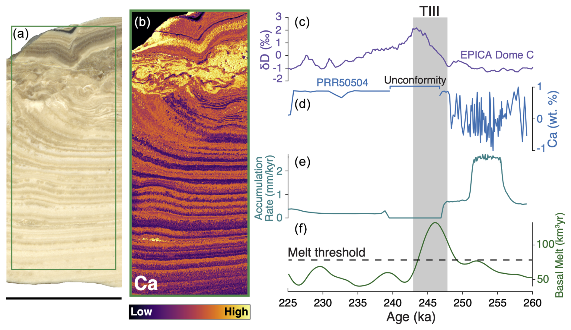
Figure 1 Sample PRR50504 formation time series versus EPICA Dome C ice core record. (a) Plain light image of sample PRR50504. Green box delineates location of the elemental map shown in panel (b). (b) Micro-XRF (µ-XRF) map of Ca in PRR50504. (c) δD measured in the EPICA Dome C ice core (Jouzel et al., 2007; Veres et al., 2013). (d) Time series of normalized Ca concentration in PRR50504. High Ca values represent calcite layers; low Ca values represent opal layers. (e) Calculated deposition rate of PRR50504. The period (247–239 ka) with a deposition rate of zero corresponds to the unconformity near the top of the sample. (f) Modeled meltwater production rates beneath Antarctica.

2.1 U-series geochronology

U-series ²³⁴U–²³⁰Th dates were produced for eight calcite layers in sample PRR50504 at the University of California Santa Cruz (UCSC) Keck Isotope Laboratory following methods described in Blackburn et al. (2020). Samples were separated into ∼ 2 mm slabs, and calcite was digested in 3 mL of 7 N HNO₃, which dissolves calcite but not opal layers. The solution was separated from undigested opal, and a mixed ²²⁹Th–²³⁶U tracer was added for isotope dilution analysis. U and Th separates were purified using ion chromatography with 1 mL columns of 200–400 mesh, AG1-X8 anion resin. Column wash acid was collected for later Sr measurements. Total procedural blanks were <10 pg for U and <25 pg for Th.

Uranium and thorium isotope measurements were conducted using the IsotopX X62 thermal ionization mass spectrometer (TIMS) housed at UCSC. Purified U and Th are loaded onto 99.99 % purity Re ribbon, in silica gel and graphite emitters, respectively. Uranium measurements were performed as a two-sequence “Fara-Daly” routine: in the first sequence, ²³⁴U (mass 266) is collected on the Daly, while ²³⁵U (mass 267) and ²³⁸U (mass 270) are collected on the high Faraday cups equipped with 1×10¹²Ω resistors. The second sequence placed ²³⁵U (mass 267) on the Daly and ²³⁶U (mass 268) and ²³⁸U (mass 270) on the high Faraday cups. The 266(Daly)/270(Faraday) composition was corrected using the Fara-Daly gain: (267Faraday/270Faraday)/(267Daly/270Faraday). Thorium was run as a metal and was measured using a peak-hopping routine on the Daly. Thorium fractionation and dead time were estimated by running NBS U-500 as a metal. Accuracy of ²³⁴U–²³⁰Th dates were tested using MIS 5e coral and compared to dates from Hamelin et al. (1991), as well as a previously dated carbonate precipitates (Frisia et al., 2017). U–Th ages were calculated using codes designed at UCSC. All ages were corrected for initial [${}^{\mathrm{230}}\mathrm{Th}{/}^{\mathrm{232}}\mathrm{Th}$] assuming a composition of 0.82 ± 0.4. Since the exact [${}^{\mathrm{230}}\mathrm{Th}{/}^{\mathrm{232}}\mathrm{Th}$]_i of our sample is unknown, we assume this ratio from the expected composition of the silicate upper crust in secular equilibrium, allowing for a departure from this composition of 50 % and propagating this uncertainty through to the final age. Decay constants for all data and models were from Cheng et al. (2000). All uncertainties are reported at 2σ, unless otherwise specified.

We constructed an age model describing age versus sample depth using Chron.jl (Keller, 2018). There we input sample height and ²³⁴U–²³⁰Th dating dates into a Bayesian Markov chain Monte Carlo model that considers the age of each layer and its stratigraphic position within the sample to refine the uncertainty of each date using a prior distribution based on the principle of superposition (Fig. S1).

2.2 Isotope analyses

2.2.1 Carbon and oxygen isotopes

Carbon and oxygen isotope ratios were measured by the UCSC Stable Isotope Laboratory using a Thermo Scientific Kiel IV carbonate device and MAT 253 isotope ratio mass spectrometer. Referencing δ¹³C${}_{{\mathrm{CO}}_{\mathrm{3}}}$ and δ¹⁸O${}_{{\mathrm{CO}}_{\mathrm{3}}}$ to Vienna PeeDee Belemnite (VPDB) is calculated by two-point correction to externally calibrated Carrara marble CM12 and carbonatite NBS-18 (Coplen et al., 2006). Externally calibrated coral Atlantis II (Ostermann and Curry, 2000) was measured for independent quality control. Typical reproducibility of replicates was significantly better than 0.05 ‰ for δ¹³C${}_{{\mathrm{CO}}_{\mathrm{3}}}$ and 0.1 ‰ for δ¹⁸O${}_{{\mathrm{CO}}_{\mathrm{3}}}$.

2.2.2 Strontium isotopes

Sr isotopic measurements were made on the TIMS at the UCSC Keck Isotope Laboratory using a one-sequence, static measurement: ⁸⁸Sr was measured on the axial Faraday cup, while ⁸⁷Sr, ⁸⁶Sr, ⁸⁵Rb, and ⁸⁴Sr were measured on the low cups. Accuracy of the ${}^{\mathrm{87}}\mathrm{Sr}{/}^{\mathrm{86}}\mathrm{Sr}$ was evaluated using standard SRM987 compared to a long-term laboratory average value of 0.71024, with a typical reproducibility of ±0.00004 ‰. The absolute standard errors for the precipitate Sr isotope measurements reported here are between $\mathrm{2.8}\times {\mathrm{10}}^{-\mathrm{5}}$ and $\mathrm{4.8}\times {\mathrm{10}}^{-\mathrm{6}}$.

2.3 Laser ablation (LA ICP-MS) elemental analyses

Laser ablation inductively coupled plasma–mass spectrometry (LA ICP-MS) analyses were conducted at the Facility for Isotope Research and Student Training (FIRST) at Stony Brook University following protocols outlined in Piccione et al. (2022). Analyses were made using a 213 UV New Wave laser system coupled to an Agilent 7500cx quadrupole ICP-MS. The National Institute of Standards and Technology (NIST) 612 standard was used for approximate element concentrations using signal intensity ratios. Laser data were reduced in Iolite software (Paton et al., 2011); element concentrations were processed with the trace-element data reduction scheme in semiquantitative mode, which subtracts baselines and corrects for drift in signal. Following acquisition, laser data representing calcite were isolated from those representing opal and detritus by subtracting points with Si concentration >100 000 ppm and with Al concentration >400 ppm.

2.4 Synchrotron X-ray fluorescence (XRF) and X-ray absorption near edge structure (XANES)

X-ray fluorescence (XRF) maps and X-ray absorption near edge structure (XANES) analyses were made at the tender energy X-ray spectroscopy (TES) Beamline 8-BM (Northrup, 2019) and at the X-ray fluorescence microprobe (XFM) Beamline 4-BM at the National Synchrotron Light Source (NSLS-II) at Brookhaven National Laboratory. At TES, incident beam energy was set to 2700 eV with Si (111) monochromator crystals and focused to a 5 × 10 µm spot size for large elemental maps and for microbeam X-ray absorption spectroscopy, and it was reduced to 2 × 3 µm for fine mapping. Samples were oriented at 45° to beam, and fluorescence was measured using a Canberra ultra-low-energy Ge detector. The 2700 eV beam stimulates fluorescence from elements Mg through S but is below the Ca K edge to avoid interference. Sulfur K-edge XANES measurements were collected over an energy of 2440–2550 eV, which stimulates fluorescence above the S K edge but is below Ca K edge to avoid interference. Energy scanning was conducted in quick on-the-fly mode, 10–30 s per scan with multiple scans at selected pixels of the elemental maps. At XFM, XRF maps were collected with the sample mounted at 45° relative to the micro-focused incident beam with a spot size of 5 × 8 µm. Data were collected using on-the-fly scanning with a 125 ms dwell time using a four-element Vortex-ME4 silicon-drift-diode detector with incident energy tuned to 17.3 keV to stimulate fluorescence from elements Ca and heavier. XANES spectra of Fe and Mn were measured by step-scanning energy across those elements' respective K absorption edges at 7.1 and 6.4 keV. Normalization and analysis of XANES spectra used the Athena software (Ravel and Newville, 2005).

2.5 Opal–calcite time series analysis

We investigated the depositional timing of finely laminated opal–calcite layers in the bottom 1.6 cm of PRR50504 through spectral analyses of time series data that describe these mineralogic transitions. Starting with the XRF element map of calcium (Fig. 2b), we measured a line scan of signal intensity across the precipitate layers to derive a spectrum representing mineralogy (i.e., high Ca layers represent calcite, low Ca layers represent opal; Fig. 2c). This spectrum was then plotted versus our age–depth model to produce a time series. To analyze the frequency of opal–calcite transitions in this time series, we used the MATLAB signal multiresolution analyzer app to generate decomposed frequency signals from the time series spectrum. The best match for the original spectra was produced with deconstructed signals with periods between 150 and 650 (Fig. 2b, c), indicating that opal–calcite layers were deposited with a centennial-scale frequency.

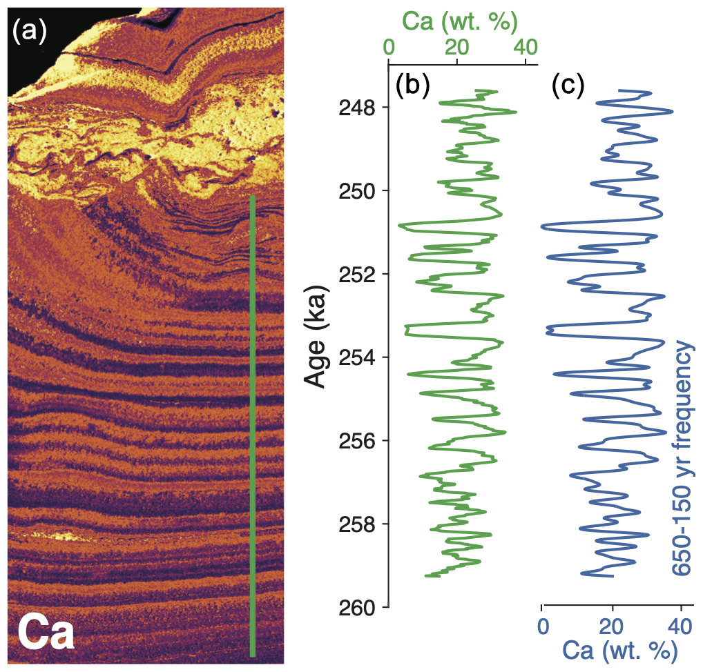
Figure 2 Pre-termination III centennial-scale opal–calcite deposition. (a) Map of Ca measured with micro-XRF (µ-XRF). Green line represents the area where the line scan was measured in panel (b). (b) Time series data of calcium concentration (wt %) in bottom segment of PRR50504. High Ca values represent calcite layers; low Ca values represent opal layers. (c) Signal multiresolution analysis of spectra in panel (b), including only periods between 650 and 150 years. The close match between this spectrum and the one in panel (b) suggests that the dominant depositional timescale of the opal–calcite cycles ranges between 650 and 150 years.

2.6 Model of subglacial meltwater production and relative iron discharge

To illustrate how Antarctic basal water melting and flux rates may have varied with climate and ice sheet fluctuations, we use a simplified model of thermal energy balance beneath the Antarctic Ice Sheet (see Supplement Sect. S1) (Fig. 1f). There are too many uncertainties, including the uncertainty in sample formation location, for us to make a meaningful attempt at simulating the specific variations that our precipitate sample has experienced. To appreciate the challenge with detailed modeling of past basal melting rates in Antarctica, one can examine the tremendous effort that it took Llubes et al. (2006) or Pattyn (2010) to derive estimates (with significant uncertainties) of melt rates beneath the modern, relatively well constrained, configuration of the Antarctic Ice Sheet (Llubes et al., 2006; Pattyn, 2010). Hence, we opt for a simplified model that captures the salient aspects of climate-driven variations in subglacial melting rates (Supplement Sect. S1). The implicit assumption in our approach is that the hydrological variations our sample experienced during its formation reflected the general subglacial hydrological conditions beneath the ice sheet.

We combine modeled subglacial meltwater production (Fig. 1f), with precipitate derived estimates of iron mobilization to explore the change in Antarctic Fe flux to the Southern Ocean across TIII. First, we assume that the modeled rate of meltwater production in the subglacial environment is a reasonable estimate of discharge rate, and thus the amount of water input to the system must be balanced by water export. We then calculate the Fe discharge rate by setting the Fe concentration of these Antarctic basal waters. Based on our precipitate Fe concentrations, parent waters had minimal Fe prior to the termination. To simulate Fe concentrations in Antarctic subglacial waters that contain dissolved oxygen and low concentrations of redox-sensitive elements, we set the concentrations of these waters equal to those of modern Subglacial Lake Whillans (2504 nM). (Vick-Majors et al., 2020). As discussed below, post-TIII precipitate chemistry suggests that metal-rich waters may form in the aftermath of glacial terminations and can affect Antarctic meltwater Fe flux. We simulate this additional Fe discharge by setting the post-TIII subglacial water Fe concentration equal to that of Subglacial Lake Whillans, with an addition of 1 %–5 % of the Fe concentration in the Blood Falls – like brine (4 × 106 nM).

3 Results and discussion

3.1 Description of precipitate mineralogy and formation mechanism

The subglacial precipitate studied here consists of alternating layers of opal and calcite, reflecting episodic shifts in precipitate parent water chemistry and/or physical conditions in the subglacial aqueous environment. Previous investigations of Antarctic subglacial precipitates with similar interspersed opal and calcite layers presented geochemical data and models suggesting that their formation is linked to cycles of freezing and flushing of basal water (Piccione et al., 2022). In the subglacial environment, opal deposition requires high concentrations of dissolved silicon (Si), likely sourced from chemical weathering of silicate bedrock and concentrated through freezing of the water body (cryoconcentration). The resulting high-Si waters produce colloidal opal in the water column, which settles on the substrate, forming a monomineralic opal layer (Piccione et al., 2022).

Silicate weathering and cryoconcentration increase the ionic strength of the fluid, but the absence of calcite in these layers suggests that the opal-forming water is undersaturated with respect to calcite, likely due to a lack of carbon. Thus, subsequent precipitation of calcite would require influx of dissolved carbon, which raises the alkalinity of the solution if this high-ionic-strength fluid is sufficiently buffered. The δ¹³C of these carbonates matches that of organic matter, suggesting that mineralization of organic matter is the most likely source of carbon in this environment (Piccione et al., 2022). As discussed further in the following section, the periodic and cyclic shifts between opal and carbonate indicate that this carbon was likely sourced via flushing of a second water from upstream, rather than in situ organic matter dissolution. We propose that the delivery of carbon occurs via flushing of carbon-rich waters into the system, shifting precipitation to calcite until the solution once again falls below the calcite saturation point (Piccione et al., 2022). Therefore, calcite accumulation (i) is minimal during times when subglacial flushing rates are slow because carbon production and delivery is low and (ii) is highest when subglacial flushing increases but (iii) can become dampened if subglacial flushing rates become so high that previously solute-rich subglacial waters are diluted with glacial meltwater.

3.2 Decreased subglacial meltwater flushing following glacial termination III

U-series data were collected in calcite along a transect from the top to the bottom of the precipitate. The calcite contained elevated uranium concentrations (1.37–3.12 ppm) and relatively low thorium concentrations (0.006–0.08 ppm), which resulted in high ${}^{\mathrm{230}}\mathrm{Th}{/}^{\mathrm{232}}\mathrm{Th}$ ratios (221–1228) and a minimal correction for detrital thorium in the final calculated ²³⁴U–²³⁰Th age. The calculated [${}^{\mathrm{234}}\mathrm{U}{/}^{\mathrm{238}}\mathrm{U}$]_i (brackets denote activity ratio; subscript ”i” denotes that this is the calculated initial ratio) ranges between 2.44 and 2.64. The spread in ${}^{\mathrm{230}}\mathrm{Th}{/}^{\mathrm{232}}\mathrm{Th}$ and [${}^{\mathrm{234}}\mathrm{U}{/}^{\mathrm{238}}\mathrm{U}$]_i likely results from heterogeneous conditions in the subglacial environment across the ∼ 25 kyr sample formation period. Error in calcite U-series geochronology can occur through open-system uranium or thorium behavior. For sample PRR50504, the eight calcite ages fall in stratigraphic order within 2σ uncertainties, corroborating the fact that the U-series system is acting as a closed system in this sample.

Based on the eight U-series measurements, we constructed a model describing age versus sample height that constrains the depositional age of PRR50504 to a 25 kyr period between 259.2 ± 2.15 and 224.8 ± 1.51 ka (Figs. 1; S1). The calcite and opal layers in the bottom section were deposited from 259.2 ± 2.15 to 247 ± 3.2 ka during the end of MIS 8. Following a depositional hiatus, the top calcite formed from 239.7 ± 2.55 to 224.8 ± 1.51 ka during MIS 7 (Fig. 1b). Based on this age model, the boundary between the top and bottom sections of the sample represents an unconformity that occurred from 247 ± 3.2 to 239.7 ± 2.55 ka, coinciding with TIII (Fig. 1). The interruption of precipitation could result from increased subglacial water flow during the termination, which would dilute subglacial waters with fresh meltwater and drive the parent solution below calcite saturation (Piccione et al., 2022) or from erosion of calcite during times of high meltwater flow (Wróblewski et al., 2017). In either case, the ∼ 7.3 kyr between TIII and the resumption of calcite precipitation represents the period over which parent waters became concentrated enough to reach calcite saturation again.

Though this subglacial precipitate records hydrologic and chemical conditions from a single location beneath EAIS, the sudden shift in precipitate textures across TIII (Fig. 1a) suggests that conditions in PRR50504 parent waters changed in response to a global climate event. Similar connections between the EAIS hydrologic system and Southern Hemisphere temperature change have been linked to catchment-scale subglacial meltwater flushing cycles driven by climate changes. (Piccione et al., 2022). To investigate the hydrologic change in PRR50504, we first focus on the alternating, 200 µm opal and calcite layers in the bottom section of the sample. Frequency analysis of the time series describing pre-TIII opal–calcite deposition shows that these mineralogic transitions occur on timescales of 150 to 650 years (Fig. 2c). There are no other glaciological (i.e., basal freezing/melting) or chemical (i.e., chemical weathering) processes that are both cyclic and can affect the basal hydrologic environment on a century scale. Therefore, century-scale pacing of opal–calcite layer formation is interpreted here to indicate that these layers resulted from subglacial meltwater flushing events in an active hydrologic system. That is, in the 15 kyr prior to TIII, ambient conditions in the subglacial environment where PRR50504 formed supported freezing of parent waters and opal precipitation, which was interrupted by centennially paced flooding of upstream waters that drove calcite precipitation. Following TIII, opal layers in PRR50504 become less frequent – with only two thin 50–200 µm black-colored opal layers deposited in the upper section of the sample – and the sample is made predominantly of red-brown calcite. Compared to the fine opal–calcite layering prior to the termination, the deposition rate of this post-TIII calcite is significantly slower (Fig. 1e), indicating that meltwater flushing to the sample formation area slowed as the climate cooled following TIII.

3.3 Greater trace metal mobility following termination III

The diminished Antarctic subglacial hydrologic activity following TIII not only slowed deposition rates in PRR50504, but also triggered a significant shift in parent water chemistry (Fig. 3). In the pre-TIII bottom section of the sample, opal and calcite contain little to no trace metals, save for one prominent layer with high Fe concentrations (Fig. 3). Elemental maps collected using micro-X-ray-fluorescence (µ-XRF) imaging show that this pre-TIII iron is concentrated in a single particulate-rich layer (Fig. 3b). Measurements of X-ray absorption near edge structure (µ-XANES) spectra on these particles indicate that they are Fe(III)-rich silicates, consistent with detrital sediments (Fig. 4b). In contrast, the portion of PRR50504 deposited after TIII shows enriched concentrations of redox-sensitive trace elements, including Fe, Mn Cu, S, and Mo, as demonstrated by laser ablation multi-collector inductively coupled mass spectrometry (LA ICP-MS) and µ-XRF analyses (Fig. 3b, c). All five elements are found in high abundance within the calcite layers (Fig. 4b), while Fe, Mn, and Cu are abundant in particles directly above the unconformity and in the two black opal layers (Fig. 3b). The enrichment of metals in both opal and calcite suggests that the observed trend in trace metals reflects higher metals in precipitate parent waters following TIII.

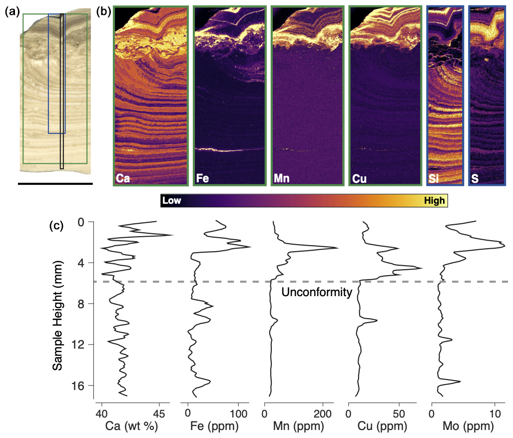
Figure 3 Elemental composition of sample PRR50504 measured with XRF and LA ICP-MS. (a) Plain light image of PRR50504. The green box delineates the location of Ca, Fe, Mn, and Cu µ-XRF maps in panel (b); the blue box delineates the location of the Si and S µ-XRF maps in panel (b); and the black box delineates the location of the LA ICP-MS analyses in panel (c). Scale bar below image is 1 cm. (b) µ-XRF maps of Ca, Fe, Mn, Cu, Si, and S. (c) LA ICP-MS Ca, Fe, Mn, Cu, and Mo concentration analyses of calcite layers in PRR50504.

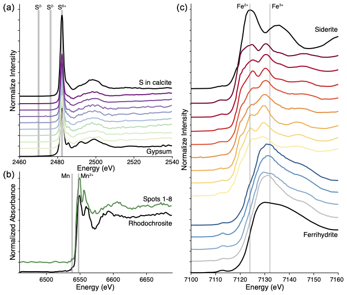
Figure 4 S, Fe, and Mn K-edge micro-X-ray absorption near edge structure (µ-XANES) spectra from PRR50504. (a) Sulfur K-edge µ-XANES spectra from eight spots in the upper section of PRR50504. All areas measured have a peak energy position that matches sulfate (S²⁺). Black spectra are sulfate-rich calcite (top) and gypsum (bottom) sulfate reference standards. (b) Mn K-edge µ-XANES spectra from eight Mn-rich spots in the upper section of PRR50504 (combined in the green spectrum) and a Mn-calcite standard (rhodochrosite, black spectrum). Both spectra have weak pre-edge peak at 6539 eV and an edge position at 6549 eV indicative of Mn²⁺ species (Schaub et al., 2023); the double-peak structure is characteristic of rhombohedral carbonate (Lee et al., 2002). (c) Iron K-edge µ-XANES spectra from 11 spots in the upper section of PRR50504 (colored red to blue) and a spectrum from three spots from the lower section of PRR50504 (combined into the single gray spectrum). Black spectra are from an Fe²⁺ reference standard (siderite, top) and an Fe³⁺ standard (ferrihydrite, bottom). Red spectra from the upper portion of the sample have peaks at 7124 and 7132 eV that indicate mixed Fe²⁺ and Fe³⁺. Blue and gray only have peaks at 7132 eV, indicating that they consist of just Fe³⁺.

High metal concentrations in opal can result from detrital inclusions or the substitution of metals such as Al³⁺, Fe³⁺, and Mn²⁺ into the Si⁴⁺ site (Gaillou et al., 2008). The opal layers above the unconformity are enriched in Fe and Mn, consistent with elevated concentrations of these metals in the parent solution. In contrast, elements like Cu and S are abundant in the post-TIII calcite but absent from the opal layers. The partition behavior of most elements in opal remains poorly constrained, making it difficult to assess whether the absence of certain elements reflects parent water conditions or other factors and limiting the ability to directly compare metal concentrations in opal versus calcite. Because element partitioning into carbonate is better understood, our discussion of parent water chemistry focuses on trace element concentrations in the calcite layers.

Calcite above the unconformity in PRR50504 is highly enriched in Fe, Mn, Cu, S, and Mo (Fig. 4). The µ-XANES spectra for S and Mn in these areas match patterns consistent with element incorporation into the calcite lattice (Fig. 5). Negative correlations between trace element concentrations and Si (Fig. S2), along with the lack of association with Al (Fig. S3), further indicate that Fe, Cu, and Mo are concentrated in the calcite rather than in detrital grains or clays. However, Fe and Cu may also be present in nanoparticles smaller than the 5 × 8 µm spot size used for XRF mapping, as Fe- and Cu-rich nanoparticles are known to form in subglacial waters (Hawkings et al., 2018; Sklute et al., 2022).

Calcite trace element concentrations often reflect parent water geochemistry or formation conditions. For example, sulfate incorporation into calcite is a function of the ${\mathrm{SO}}_{\mathrm{4}}^{-}/{\mathrm{CO}}_{\mathrm{3}}$ ratio of the parent fluid (Staudt and Schoonen, 1995) and is substituted into the calcite lattice at the carbonate ion site (Kontrec et al., 2004). Mn²⁺, Fe²⁺, and Cu²⁺ substitute for Ca²⁺ in the calcite lattice (Dromgoole and Walter, 1990; Schosseler et al., 1999). Mn-rich carbonate formation tends to occur in low-O₂ settings, where Mn enrichment can develop via reduction of Mn oxides, and may be associated with processes such as sulfur cycling or Fe oxidation in euxinic or ferruginous environments (Wittkop et al., 2020). Such processes have been observed in the Ca–Cl brines within Lake Vanda in Wright Valley, Antarctica (Webster, 1994). Similarly, formation of Fe-rich carbonates requires high Fe concentrations in anoxic or ferruginous conditions (Jiang and Tosca, 2019), while the formation and incorporation of metal-rich nanoparticles would also be indicative of suboxic to anoxic subglacial conditions (Hawkings et al., 2018). Molybdenum incorporation in calcite most often occurs through adsorption onto crystal surfaces rather than in the lattice (Midgley et al., 2020).

Mobilization of redox-sensitive elements beneath ice sheets has been attributed to suboxic or anoxic fluids where chemolithotrophic organisms drive chemical weathering of trace-metal-bearing phases (e.g., sulfides, Fe or Mn oxides) (Wadham et al., 2010). In PRR50504, we use Fe, Mn, and S K-edge µ-XANES spectra to explore the redox conditions in parent waters that led to the apparent trace metal cycling following TIII. First, Mn K-edge µ-XANES spectra show that Mn-rich areas at the top of the sample are a Mn²⁺ carbonate (Fig. 4c), formation of which requires reducing conditions where dissolution of Mn oxides from the bedrock substrate drive high concentrations of Mn²⁺ in solution (Calvert and Pedersen, 1993). Second, Fe and Mn concentrations are of similar magnitude (Fig. 3c), indicating that both Fe and Mn were highly concentrated in the parent waters. Based on Fe K-edge µ-XANES spectra, the detritus directly above the unconformity is mixed Fe²⁺ and Fe³⁺ silicates (Fig. 4b), consistent with glaciogenic sediments weathered in anoxic environments (Hawkings et al., 2018). Third, S K-edge µ-XANES spectra show that high concentrations of sulfur (Fig. 3b) are present as sulfate (Fig. 4a), with no evidence for precipitated sulfides, meaning that parent waters did not become sufficiently anoxic to drive sulfate reduction (i.e., sulfidic or euxinic conditions). Elevated Cu concentrations in the top of the sample coincide with high Mn and Fe concentrations (Figs. 3b, c; S6), consistent with Fe–Mn-oxide dissolution in a manganous or ferruginous environment (Scott and Lyons, 2012; Tribovillard et al., 2006). Finally, molybdenum is soluble in oxygenated waters (Boothman et al., 2022) and can adsorb onto Mn oxides (Scott and Lyons, 2012). As the solution transitions to reducing conditions, Mn oxides are dissolved, leading to both elevated Mo and Mn, as observed in PRR50504 (Fig. 3c). Collectively, these data show that the subglacial waters were near the redox boundary between manganous and ferruginous conditions during the deposition of the top section of the sample, driving redox-sensitive elements into solution.

Oxygen levels in the subglacial environment are controlled by the influx of oxygen from melted glacial ice (Lipenkov and Istomin, 2001) and its consumption through aerobic oxidation reactions (Michaud and Priscu, 2023; Vick-Majors et al., 2016). Direct sampling of subglacial and ice-covered lakes in Antarctica reveals suboxic conditions driven by microbial oxygen consumption (Christner et al., 2014) and indicates that oxygen is periodically replenished by upstream glacial melt (Faucher et al., 2021; Vick-Majors et al., 2016). These waters are along the ice sheet periphery, where subglacial meltwater flushing occurs on week-to-month timescales (Siegfried and Fricker, 2018). Even in these hydrologically active regions of the basal environment, oxygen consumption would deplete an oxic water body within years (Vick-Majors et al., 2016). In the subglacial environments beneath the interior of the ice sheet, where residence times can be centuries to millennia (Livingstone et al., 2022), oxygen levels are likely tied to the rates of melting and flow of basal water, which control the delivery of oxygen. On this basis, we attribute the transition in redox across TIII in PRR50504 (Fig. 3) to a shift from frequent to less frequent meltwater flow as demonstrated by the sample accumulation rate (Fig. 1e). In the next section, we test this hypothesis and discuss potential climate drivers for this change in subglacial water flushing rate across TIII.

3.4 Subglacial trace metal mobilization linked to climate through basal flushing rates

The change in subglacial water flushing rate and metal concentrations recorded in PRR50504 across TIII demonstrates a link between subglacial meltwater chemistry and glacial–interglacial climate cycles. The most likely forcing capable of such a shift is an ice dynamic response, which has a dominant influence on basal meltwater flow (Hayden and Dow, 2023). The precipitate record presented here reflects conditions in a single location beneath the David Glacier catchment, and with this dataset alone, it is not possible distinguish between local versus catchment-scale change in basal chemistry. However, as discussed below, changes in ice sheet motion following a termination could affect basal chemistry across the broader catchment. To fully support the hypothesis of a large-scale change in subglacial trace metal mobility would require observing this phenomenon in more samples from David Glacier and in areas around Antarctica, which is beyond the scope of this paper. Nevertheless, we explore the potential connection between large catchment-scale ice dynamics and basal meltwater flow using a simplified model of thermal energy balance beneath the Antarctic Ice Sheet (see Supplement Sect. S1).

We simulate the evolution of subglacial meltwater production across the period of time covered by PRR50504 (259.5 to 225 ka) (Fig. 1f). This model estimates how shear heating and conductive heat loss evolve during climate fluctuations and drive the heat budget of the ice–bed interface (see Supplement Sect. S1). Across the period of PRR50504 formation, the deposition rate (Fig. 1d) and depositional frequency of opal–calcite layers (Fig. 2) respond to trends in subglacial meltwater production. From 258 to 251 ka, increased meltwater availability leading up to TIII (Fig. 1e) drove the frequent centennial-scale opal–calcite transitions (Fig. 2) and higher deposition rates (Fig. 1e). At 251 ka the subglacial meltwater production reached a threshold value that was large enough to dilute the precipitate parent water to the point where it was no longer saturated with respect to opal and calcite, causing precipitate formation to cease (Fig. 1e). Following the TIII, meltwater production decreased rapidly, isolating PRR50504 parent waters along the periphery of the ice sheet from upstream subglacial meltwater. Eventually, this isolation allowed the parent water to again become saturated with respect to calcite and precipitate formation to restart, but the change in meltwater delivery rate resulted in reducing conditions and distinct parent water chemistries.

The trends in subglacial flushing rates across TIII evident in PRR50504 (Figs. 1; 2) are interpreted here as resulting from climate-driven changes in the ice sheet motion that modulate subglacial meltwater and oxygen supply through their impact on conductive heat loss and basal shear heating (Fig. 1e) (see Supplement Sect. S1). Similar climate-forced fluctuations in Antarctic subglacial hydrologic activity have been reported from precipitate samples covering a range of Late Pleistocene climatic conditions outside of terminations (Piccione et al., 2022). Pleistocene glacial terminations trigger thinning along the EAIS periphery (Wilson et al., 2018). Consequent subglacial shear heating and steepening of the ice surface gradient may have caused the highest influx of meltwater to the formation location of PRR50504 during TIII (Fig. 1e). Immediately following terminations, ice motion slowed, but slow ice surface accumulation rates behind the Transantarctic Mountains imply that it takes many millennia to re-establish peak glacial ice thickness and extent. This post-termination period of slow ice motion, thin ice, and low ice surface slopes along the Antarctic margins produces the lowest rates of subglacial meltwater production (Fig. 1e), and we interpret it as the cause of subglacial freezing and diminished meltwater flushing intensities recorded in our sample.

3.5 Potential climate-driven trends in Antarctic trace metal discharge to the Southern Ocean

The evidence presented here for high trace metal concentrations in subglacial waters beneath the EAIS suggests that metal-rich fluids formed in the subglacial aqueous system in which PRR50504 precipitated. Given the numerous instances and geographic distribution of metal-rich subglacial waters emanating from beneath ice in Antarctica (Annett et al., 2015; Forsch et al., 2021; Monien et al., 2017), the hydrologically isolated, suboxic environments that produce these metal-rich fluids are potentially ubiquitous in Antarctic basal environments, particularly in its peripheral regions where lower ice thicknesses favor basal freezing (e.g., Pattyn, 2010). The transition in PRR50504 from redox element-poor meltwater prior to TIII to metal-rich parent waters after TIII indicates that high metal concentrations can occur naturally in subglacial environments in response to changing hydrological connectivity or isolation, which control the availability of oxygen in subglacial waters.

Modern Antarctic basal waters have a range of Fe concentrations, ranging from Fe-poor, oxygenated waters (Vick-Majors et al., 2020) to suboxic, Fe-rich brines (Lyons et al., 2019). Modeling studies estimate modern Fe discharge rates of up to 1.4 Gmol yr⁻¹ by extrapolating these observed water compositions to the ice sheet scale (Hawkings et al., 2020), suggesting that subglacial meltwater may play an important role in fertilizing Southern Ocean ecosystems. The precipitate record presented here offers a well-dated geologic record illustrating how subglacial trace metal cycling may vary in response to global climate fluctuations, permitting similar estimates of Antarctic Fe discharge to the Southern Ocean on glacial–interglacial timescales.

We evaluate Antarctic Fe discharge rate across TIII by integrating results from our simplified model of meltwater discharge rate (Fig. 1e) with estimates of Fe concentration of subglacial waters, informed by the fluctuations in trace metal mobility observed in our subglacial precipitate record (Fig. 5c). Similar to previous models of Antarctic Fe discharge flux (Hawkings et al., 2020), this calculation is limited by the necessity to extrapolate observed water compositions to the continent-wide basal hydrologic system. Hence, this exercise represents a qualitative investigation of the sensitivity of Antarctic Fe flux to a range of meltwater Fe concentrations, representing the possible influence of climate-driven changes in subglacial trace metal mobility on Antarctic Fe discharge to the Southern Ocean.

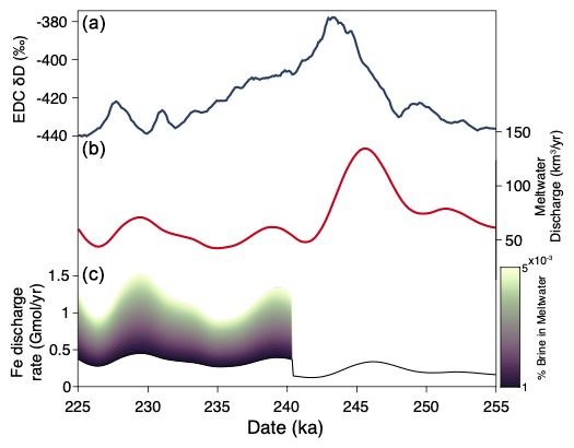
Figure 5 Simplified model of Antarctic subglacial Fe flux across TIII. (a) δD measured in the EPICA Dome C ice core (Jouzel et al., 2007; Veres et al., 2013). (b) Modeled meltwater production rates beneath Antarctica. (c) Modeled Antarctic subglacial Fe flux. Color scale represents the fraction of subglacial meltwater made up of Blood Falls-like brine compositions.

Prior to TIII, PRR50504 parent waters had low trace metal concentrations (0–10 ppm Mn; 0–15 ppm Fe; 0–10 ppm Cu), indicative of oxidized aqueous conditions. To simulate discharge of these Fe-poor waters, we set subglacial meltwater Fe concentration to those in modern Subglacial Lake Whillans (2504 nM Fe) (Vick-Majors et al., 2020) for the 15 kyr prior to TIII. The calculated Fe flux aligns with meltwater discharge rates in this pre-TIII period, increasing from 0.15 Gmol yr⁻¹ before the termination up to 0.33 Gmol yr⁻¹ during the termination (Fig. 5c). These values are consistent with previous estimates of Fe discharge that assume lower Fe concentrations in subglacial waters (Hawkings et al., 2014; Hodson et al., 2017) but are below an estimate of 1.4 Gmol yr⁻¹ made using Fe concentrations of Subglacial Lake Mercer (Hawkings et al., 2020).

As the climate cooled following TIII, PRR50504 parent waters became manganous/ferruginous. To represent the subglacial formation of Fe-rich waters in the 10 kyr after TIII, we set subglacial meltwater Fe concentrations for this period equal to a mixture of Subglacial Lake Whillans compositions plus a varying portion of Blood Falls brines. It is impossible to know the true magnitude of metal accumulation in subglacial waters across the continent. However, because our record shows metal accumulation in regions of the subglacial hydrologic system that become periodically isolated in response to glacial–interglacial cycles, we add brines only in the regions of the subglacial environment that can freeze and thaw on glacial–interglacial environments. Dawson et al. (2022) model this thawable region of the ice sheet bed. Based on their conservative estimates, approximately 0.5 %–1.5 % of the ice sheet base is susceptible to transition between freezing and thawing across period of major climate transition. To simulate subglacial metal accumulation on a catchment scale, we approximate that between 0.2 % and 1 % of waters in these thawable regions may accumulate metal in response changing ice dynamics following a termination. Therefore, we set the proportion of high concentration brine, similar to present-day Blood Falls, in post-TIII simulation to 0.001 % and 0.005 % of the total subglacial water.

The magnitude of Fe discharged from beneath the Antarctic Ice Sheet is highly sensitive to this increase in meltwater Fe concentration, with the average Fe flux maintaining peak termination values of approximately 0.3 Gmol yr⁻¹ when just 0.001 % of subglacial waters contain Fe concentrations equal to Blood Falls values. Total Fe flux increases by about 0.2 Gmol yr⁻¹ for every 0.001 % increase in the fraction of basal water made up of Blood Falls-like brine, increasing by an order of magnitude when subglacial waters contain 0.005 % brine (Fig. 5c). We stress that these Fe discharge estimates are meant to be schematic representations of the potential effect of climate-driven metal accumulation in subglacial waters. Ultimately, they demonstrate that a catchment-scale increase in trace metal mobility beneath the Antarctic Ice Sheet following glacial terminations could plausibly influence the subglacial meltwater Fe flux to the Southern Ocean.

The calcite layers in PRR50504 have a range of [${}^{\mathrm{234}}\mathrm{U}{/}^{\mathrm{238}}\mathrm{U}$]_i values between 2.42 and 2.64, indicating fluid residence times on the order of centuries to millennia (Blackburn et al., 2020). These prolonged residence times suggest that basal water flow in these upper regions of the David Glacier catchment are significantly slower than the more active peripheral regions. Consequently, the discharge of metal-rich fluids from the subglacial environment may lag behind their formation by several thousand years – a delay not accounted for in our Fe discharge model.

Parent water compositions from PRR50504 represent conditions in just one area of the subglacial environment. Therefore, Fe flux estimates are intended only to schematically illustrate the relative change in Fe discharge that may occur due to the emergence of widespread suboxic basal conditions following glacial terminations. However, the transition from centennial-scale subglacial flushing in PRR50504 parent waters before TIII to hydrologically more isolated conditions post-termination stems from a shift in the Antarctic basal hydrologic system in response to ice dynamic changes following the TIII. Previous studies have noted a comparable response of subglacial waters to Southern Hemisphere climate events, evident in various locations across the EAIS, indicating a catchment-wide phenomenon (Piccione et al., 2022). Therefore, the hydrologic shift that drove increased trace metal mobility following TIII may have occurred in other areas along the Antarctic periphery and thus may significantly increase Fe flux to the Southern Ocean during this period.

The precipitate record presented here demonstrates significant changes in subglacial trace metal mobility across a glacial termination, which may lead to large variations in the influx of limiting nutrients (e.g., Fe and Mn) to the Southern Ocean during a transition from interglacial to glacial conditions. Iron sourced from the Antarctic basal environment has been shown to be highly bioavailable, meaning that this meltwater flux can enhance marine productivity in regions where it is discharged (Hawkings et al., 2014, 2018). In the Antarctic zone of the Southern Ocean, nutrient supply is influenced from above (i.e., dust, iceberg-rafted detritus, and Antarctic meltwater) and below (i.e., upwelling of nutrient-dense bottom waters). Elemental and isotope analyses of marine sediment records from the Antarctic zone reveal that a shift from high upwellings during the warmest climate periods to stratification during glacial periods is the main driver of changes in primary productivity on glacial–interglacial cycles (Sigman et al., 2021; Studer et al., 2015). As stratification increases in the Antarctic zone, nitrate consumption in the surface ocean becomes more complete, suggesting the need for additional iron sources beyond deep marine Fe (Studer et al., 2015). While current data do not allow for an unequivocal identification of these Fe sources, increased Fe flux from Antarctic meltwater during climate cooling represents a potential origin for these nutrients.

4 Conclusions

A chemical precipitate from Elephant Moraine, East Antarctica, records a shift to slower subglacial meltwater flow and increased concentrations of redox-sensitive elements, including Fe and Mn, in subglacial waters beneath the David Glacier catchment following TIII. Prior to the termination, frequent flushing of upstream basal water supplied oxygen to this location. After the termination, reduced connectivity led to more isolated subglacial water, driving suboxic, ferruginous, and manganous conditions that promoted elevated trace metal concentrations. The post-TIII geochemical conditions preserved in PRR50504 demonstrate that suboxic water enriched in Fe and other transition metals can naturally develop in subglacial environments. We hypothesize that this increase in metal mobility resulted from an ice dynamic response to TIII that altered basal water flushing.

The precipitate record present here describes conditions in a single location beneath the David Glacier catchment. However, changes in ice sheet motion following a termination may affect the broader catchment. Reduced ice motion, shallower ice sheet surface slopes, and thinner ice following terminations can diminish subglacial meltwater production and flushing, leading to increased hydrologic isolation of subglacial waters on the ice sheet periphery from the broader hydrologic system in the ice sheet interior. Our record demonstrates that the consequent reduction in oxygen supply to peripheral subglacial waters can drive manganous/ferruginous conditions and high concentrations of trace metals in subglacial waters.

Collectively, our data suggest that climate-driven changes in ice motion may regulate trace metal mobility beneath the Antarctic Ice Sheet by altering the intensity of subglacial flushing, which in turn affects oxygen availability in peripheral subglacial waters. Based on observations from the David Glacier catchment, we hypothesize that trace metal mobility in Antarctic subglacial meltwaters peaks beneath a thinned, slow-moving ice sheet during the transition from interglacial to glacial periods. Warm climate periods promote increased subglacial meltwater production and flushing, leading to more oxygenated conditions and reduced mobility of redox-sensitive elements. Notably, while subglacial water discharge may be more voluminous during terminations than afterward, these waters may be more diluted in Fe and other nutrients. Given the potential for Antarctic meltwater discharge to fertilize Southern Ocean ecosystems (Death et al., 2014), our dataset linking subglacial trace metal flux to climate-driven meltwater production has important implications for the role of Antarctic micronutrients in the carbon cycle over glacial–interglacial timescales. Specifically, our findings suggest that Antarctic subglacial metal discharge may be highest as climate transitions to glacial periods, potentially enhancing carbon burial in the Southern Ocean and contributing to atmospheric CO₂ drawdown, reinforcing long-term cooling trends.