Fine-scale variability in iceberg velocity fields and implications for an ice-associated pinniped

Icebergs found in proglacial fjords serve as important habitats for pinnipeds in polar and subpolar regions. Environmental forcings can drive dramatic changes in the overall reduction in ice coverage across fjords in the circumpolar regions, with implications for pinnipeds that use ice for critical life-history functions, including pupping and molting. To better understand how pinnipeds respond to changes in iceberg habitat, we combine (i) iceberg velocity fields over hourly to monthly timescales, derived from high-rate time-lapse photogrammetry of Johns Hopkins Glacier and Inlet, Alaska, with (ii) aerial photographic surveys of harbor seals (Phoca vitulina richardii) conducted during the pupping (June) and molting (August) seasons. Iceberg velocities typically followed a similar diurnal pattern: flow was weak and variable in the morning and strong and unidirectional in the afternoon. The velocity fields tended to be highly variable in the inner fjord across a range of timescales due to changes in the strength and location of the subglacial outflow, whereas, in the outer fjord, the flow was more uniform, and eddies consistently formed in the same locations. During the pupping season, seals were generally more dispersed across the slow-moving portions of the fjord (with iceberg speeds of <0.2 m s⁻¹). In contrast, during the molting season, the seals were increasingly likely to be found on fast-moving icebergs in or adjacent to the glacier outflow plume. The use of slow-moving icebergs during the pupping season likely provides a more stable ice platform for nursing, caring for young, and avoiding predators. Periods of strong glacier runoff and/or katabatic winds may result in more dynamic and less stable ice habitats, with implications for seal behavior and distribution within the fjord.

1 Introduction

Ice, including sea ice and icebergs, provides an important habitat for marine mammals in subpolar and polar regions (Kelly, 2001; Laidre et al., 2015). For pinnipeds, ice provides a substrate for pupping, nursing young, avoiding predators, and reducing the likelihood of disease transmission (Fay, 1974). Given the overall reduction in ice coverage in the circumpolar regions and the reliance of pinnipeds on ice habitat (e.g., Fay, 1974; Kelly, 2001; Laidre et al., 2015; Gulland et al., 2022), an understanding of ice dynamics and variability across multiple spatial and temporal scales is essential for projecting how changes in climate may influence the distribution, abundance, behavior, and energy expenditure of pinnipeds within fjord regions.

In Alaska, tidewater glaciers produce icebergs that are used by harbor seals (Phoca vitulina richardii), the most widely distributed pinniped in the Northern Hemisphere. Icebergs in tidewater glacier fjords serve an important ecological function by providing a stable and extensive platform for critical life-history functions, including birthing and caring for newborn pups, molting, and predator avoidance. Icebergs may provide benefits over terrestrial habitats by providing a stable platform for nursing young that is not subject to tidal fluctuations and by reducing the risk of predation (Blundell et al., 2011). Although the availability of icebergs in fjords is dynamic, harbor seals exhibit high fidelity to tidewater glacier fjords during the pupping and molting seasons (Womble and Gende, 2013), representing some of the largest seasonal aggregations of harbor seals in the world (Jansen et al., 2015).

In Southeast Alaska, within the ancestral lands of the Tlingit people, Sít' Eetí Geeyi (or what is currently known as and hereafter referred to as Glacier Bay), harbor seals are monitored to assess their abundance and distribution. Aerial surveys are conducted six to eight times per year during the pupping (June) and molting (August) seasons (Womble et al., 2020, 2021). The surveys also provide important information regarding the ice habitat used by seals (McNabb et al., 2016; Womble et al., 2021; Kaluzienski et al., 2023); however, the aerial photographic methods were designed to estimate the abundance of seals over broad temporal and spatial scales (Ver Hoef and Jansen, 2015). While it is well-documented that tidewater glacier fjords provide important habitats for harbor seals, we lack an understanding of the physical processes and environmental factors that influence the fine-scale variability of iceberg habitats in the fjord and how this variability influences the distribution and behavior of seals.

Recent advances in camera and computer technologies have enabled the development of tools for tracking fine-scale spatial and temporal variability in iceberg habitat in tidewater glacier fjords with time-lapse photography (Kienholz et al., 2019) over time periods of minutes to years. Here, we use the methods in Kienholz et al. (2019) in order to characterize iceberg velocity fields during summer in Tsalxaan Niyaadé Wool'éex'i Yé (or what is currently known as and is hereafter referred to as Johns Hopkins Inlet), which is located in the northwestern corner of Glacier Bay (Fig. 1), and to relate the velocity fields to the abundance and distribution of seals within the fjord.

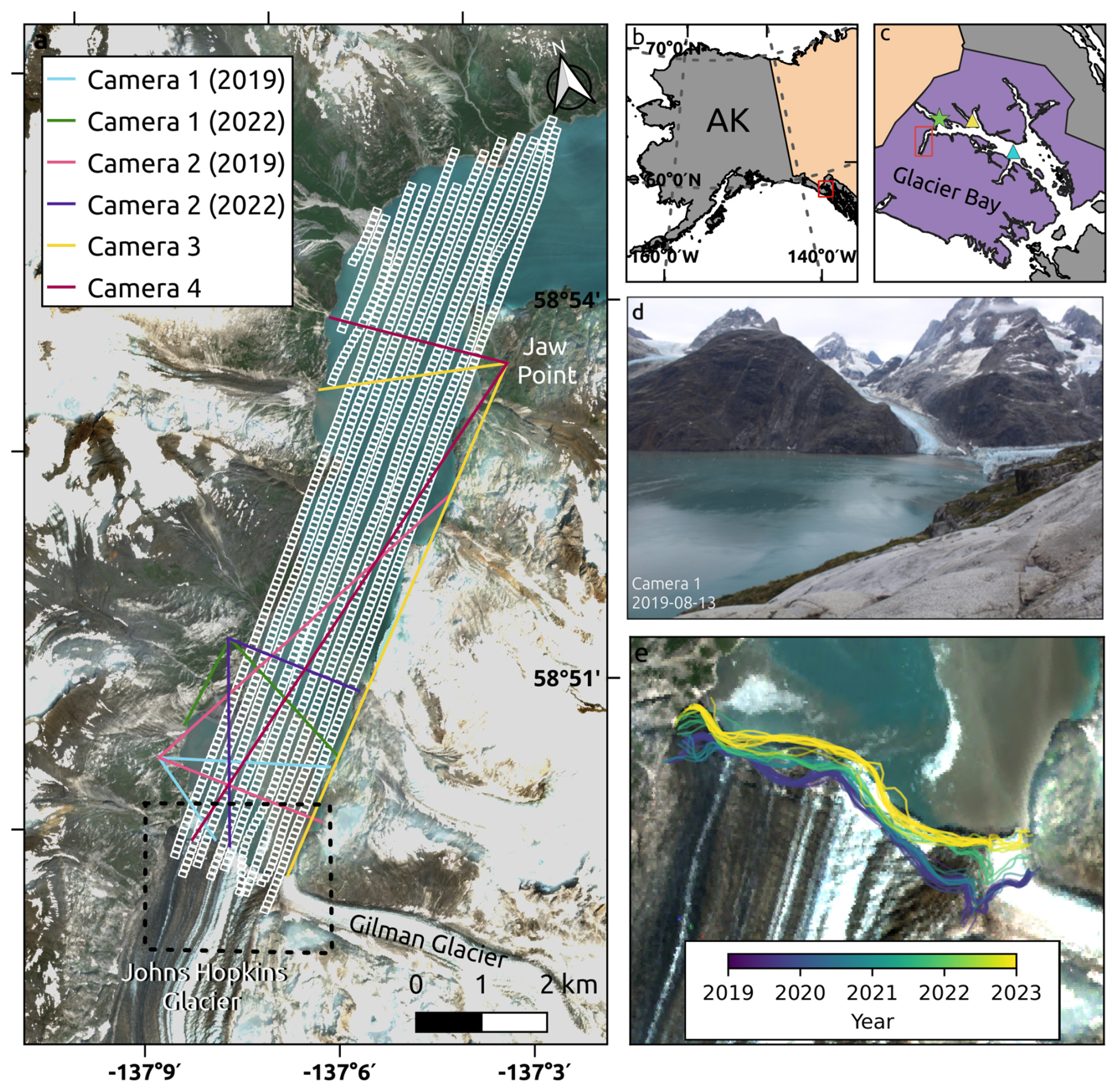
Figure 1 Map of the study site showing (a) Johns Hopkins Inlet and Glacier Bay and their location within (b) Alaska and (c) Glacier Bay National Park and Preserve. In (a), small white boxes indicate image footprints from an aerial survey flown on 29 July 2019, and colored lines denote each time-lapse camera's field of view. In (c), the green star indicates Tarr Inlet tidal station, and the yellow and blue triangles indicate Queen Inlet and Lone Island weather stations, respectively. (d) Example photos from camera 1, taken in 2019. The background image in (a) is a Sentinel-2 image from 2023 with the Alaska Albers projection (EPSG:3338). (e) Terminus positions for Johns Hopkins Glacier and Gilman Glacier during the summers of 2019–2023.

2 Study area and methods

Johns Hopkins Inlet (Fig. 1) is a tidewater glacier fjord in Glacier Bay National Park and Preserve in Southeast Alaska. We focus on the portion of the fjord that extends from Johns Hopkins Glacier to Jaw Point, which is about 9 km long and 1.5–2 km wide. Johns Hopkins Glacier, the primary tidewater glacier feeding into the fjord, reached a minimum extent in the 1920s following the disintegration of the Glacier Bay Icefield (Hall et al., 1995); it has since advanced 2 km and thickened by over 100 m in its lower reaches (Larsen et al., 2007; McNabb and Hock, 2014). In recent years, shoaling of the glacier's end moraine has reduced the iceberg flux into the fjord, thereby reducing the ice habitat for seals (Kaluzienski et al., 2023). Johns Hopkins Inlet is also fed by Gilman Glacier, whose terminus coalesces with that of Johns Hopkins Glacier. Gilman Glacier is an order of magnitude smaller than Johns Hopkins Glacier by area and is more stable, having advanced by about 200 m over the last century (McNabb and Hock, 2014). Thus, the impact of Gilman Glacier on iceberg production and habitat is relatively small compared to that of Johns Hopkins Glacier.

2.1 Time-lapse cameras

We deployed four time-lapse cameras in Johns Hopkins Inlet during the summers of 2019, 2021, and 2022. Due to camera malfunctions and a lack of overlapping aerial surveys in 2021, we focus exclusively on the data collected in 2019 and 2022. The time-lapse camera systems consisted of 18 mm Canon Rebel T3 or T5 single-lens reflex (SLR) cameras that were controlled by Harbortronics DigiSnap intervalometers. Two cameras were co-located in the inner fjord (<3 km from the glacier), and two cameras were co-located at Jaw Point (∼8.5 km from the glacier, Fig. 1). We changed the location of the cameras in the inner fjord after the 2019 season to a site that is more accessible and that has a better view of the glacier. The cameras were installed on survey-grade tripods that were stabilized with large piles of rocks, oriented to collectively observe the entire fjord and to have some overlap across photos, surveyed with geodetic-quality GNSS receivers (Emlid Reach RS2+), and programmed to take photos every minute for 14–16 h each day from June to September. One camera system malfunctioned each season due to either disturbance from terrestrial wildlife (e.g., bears) or electrical issues. Additionally, on six separate occasions, heavy fog or wind-driven rain obscured the camera lens, affecting time-lapse image data quality.

We calculated iceberg velocities from the time-lapse photos using the workflow described in detail in Kienholz et al. (2019), which involved building camera models, tracking features, and using the camera model to translate pixel displacements into map coordinates. We used a simple, planar camera model that has four free parameters: yaw, pitch, roll, and focal length (Krimmel and Rasmussen, 1986). We determined these parameters by digitizing the fjord waterline in a representative photo and projecting it into map-view coordinates using an initial guess for each of the four free parameters. The parameters were then iteratively adjusted to minimize the distance between the projected waterline and the waterline observed in a coincident Landsat 8 image. The process required knowledge of the camera's location, which was known from the GNSS surveys, and of its elevation relative to sea level. The GNSS solutions provided the camera's ellipsoidal elevation. We determined the ellipsoidal sea level elevation by shifting the NOAA tide prediction curve for the nearby Tarr Inlet (https://tidesandcurrents.noaa.gov/noaatidepredictions.html?id=9452749, last access: 2 August 2024) so that it agreed with the local ellipsoidal sea level elevations from IceSAT-2 ATL06 data (Smith et al., 2023). Comparison between the tide prediction and previous in situ tide measurements showed good agreement with the timing and magnitude of the tides in Johns Hopkins Inlet.

Once the camera models were determined, we applied a high-pass filter to the images, identified features with the Shi–Tomasi algorithm (Shi and Tomasi, 1994), and tracked the features with the Lucas–Kanade sparse-optical-flow algorithm (Lucas and Kanade, 1981) as implemented in OpenCV (https://opencv.org, last access: 20 November 2024). To filter erroneous calculations, we tracked features over four successive images and excluded any features that could not be tracked over all four images. The pixel displacements were then converted into map view; changes in tidal elevation were accounted for during this conversion. The resulting sparse-velocity field was gridded and used to create streamline plots and to plot velocity transects. Kienholz et al. (2019) demonstrated that this workflow can produce velocities with errors of less than 0.1 m s⁻¹ and that the error becomes smaller when the velocity fields are temporally averaged. In addition, they also demonstrated that small icebergs, such as those found in Johns Hopkins Inlet, serve as good tracers of surface water currents.

2.2 Aerial photographic surveys

Aerial photographic surveys have been conducted in Johns Hopkins Inlet since 2007 during the harbor seal pupping (June) and molting (August) periods (Womble et al., 2020, 2021). Typically, six to eight surveys are conducted each summer. For our time period of interest, aerial and time-lapse surveys overlapped during the pupping season (June) in 2019 and the molting season (August) in 2022. During 2019, the surveys were conducted from a de Havilland Canada DHC-2 Beaver single-engine high-winged aircraft (Ward Air Inc., Juneau, Alaska) following the methods developed by Jansen et al. (2006) and Ver Hoef and Jansen (2015). The aircraft was flown at ∼304 m and ∼90–95 kt along 12 established transects. The transects were spaced 200 m apart, were oriented perpendicularly to the terminus of Johns Hopkins Glacier, and spanned the length of the fjord from the terminus of the glacier to the opposite end of the fjord. During the 2019 aerial surveys, non-overlapping digital photographic images were taken directly under the plane using a vertically aimed digital single-lens reflex (DSLR) camera (Nikon D2X, 12.4 megapixel; Shinagawa, Tokyo, Japan) with a 60 mm focal length lens (Nikon AF Micro-NIKKOR, 2.8D). The camera was attached to a tripod head and mounted to a plywood platform that was secured in the belly porthole of the aircraft. The camera captured an image every 2 s using a digital timer (Nikon MC36) operated by an observer. The firing rate and spacing of the transects allowed for a gap between images of 15 m end to end and 70 m side to side to ensure that the images were separated from one another and that the seals were only sampled once. Each digital photograph (3216 pixel×2136 pixel JPEGs) covered approximately 80 m×120 m at the surface of the water, with a resolution of ∼3.24 cm pixel⁻¹. An onboard global positioning system (Garmin 76 CSX) was used to record the track line and position of the plane along the transects at 2 s intervals. The surveyed area encompasses approximately 48 % of the study area.

No surveys were conducted in 2020, and challenges associated with transitioning to a new camera system in 2021 precluded the collection of nadir photos that could be georeferenced. During 2022, aerial photographic surveys were conducted using a lightweight camera pod (WaldoAir XCAM Ultra50) that was attached to the wing strut of the aircraft (Cessna 206). The camera pod consisted of two Canon 5DS R 50.6 MP RGB cameras with a fixed-zoom 50 mm $f/\mathrm{1.4}$ lens, an integrated GPS unit, and a micro-controller to trigger capture events. The two cameras in the pod were synchronized by WaldoAir software and were programmed to capture images every 2 s. The width of each captured image was 470 m×159 m, with an altitude of ∼293 m, resulting in a resolution of ∼2.75 cm pixel⁻¹. Due to the larger photo footprint, only four transects were needed to cover an area similar in size to previous surveys, with an approximate distance of ∼210 m between transects. While the area coverage is similar between years, the 2022 data have larger horizontal gaps in terms of coverage (Fig. 2). Any overlap in the photo footprints was removed prior to image analysis to ensure that seals were not double-counted.

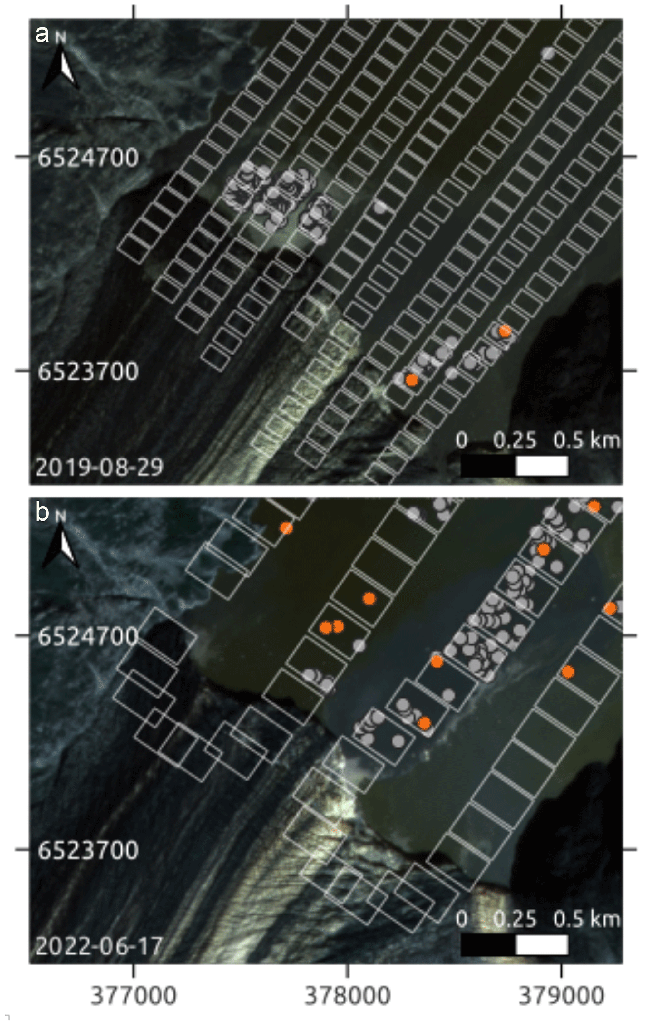
Figure 2 Footprints of aerial photographs in the terminus region during the 2019 and 2022 surveys. Orange and gray dots represent seals identified in the water and hauled out onto icebergs, respectively. Background images were taken by the Planet satellite on (a) 29 August 2019 and (b) 21 August 2022 and projected onto WGS84 UTM Zone 8N (EPSG:32608). Images from 2022 were visually inspected by a trained observer to account for and remove any overlap and to ensure that double-counting of seals did not occur. Images ©2019 and 2022 Planet Labs.

The latitude, longitude, and altitude from the track line were written to the EXIF headers of each image using RoboGEO V6.3 (Pretek Corporation, Christian, Tennessee, USA). Images from each survey were embedded as a raster layer in an ArcGIS project using ArcGIS (ESRI) and R (R Core Team 2017). Each photograph was examined by a trained observer using digital photographic software (ACDSEE Pro 4), and each seal was marked as a point feature in an ArcGIS shape file. After all seals were marked, “footprints” delineating the extent of each image were generated as polygons in a separate shape file. During the pupping season, distinct shapefiles were created for pups and non-pups. In the molting season, all seals were classified as non-pups in a single shapefile as pups had grown in size and mass, making them indistinguishable from adults.

Further details on the survey methods can be found in Womble et al. (2020). Aerial surveys were conducted under NOAA Fisheries Marine Mammal Protection Act (MMPA) permit nos. 358-1787-00, 358-1787-01, 358-1787-02, and 16094-02.

2.3 Relating seal distributions to fjord conditions

The speed of an iceberg that a seal is hauled out on depends on both the background flow speed of the fjord and the iceberg's location within the fjord. In order to quantify the likelihood of a seal being found on an iceberg or on the surface of relatively fast- or slow-moving water, we compare the velocity distribution of the seals to the background velocity distribution of the fjord. We first calculated the average iceberg velocity within each 50 m×50 m grid cell during the 3 h window of each aerial survey (“fjord velocity”) and then associated each seal with the velocity of the grid cell that it was located within (“seal velocity”). We next averaged the fjord velocity across each of the surveys during the 2019 molting and 2022 pupping seasons. These data were then used to compute complementary cumulative distribution functions (CCDFs), which indicate the likelihood that speed V of a randomly selected grid cell or seal will have a speed that is greater than v.

2.4 Auxiliary and meteorological data

To better understand fjord conditions during our aerial photographic surveys, we supplemented aerial surveys with 3 m resolution optical satellite imagery from PlanetScope, obtained through NASA's Commercial Satellite Data Acquisition Program (Planet Team, 2017) when available (Fig. 1). In particular, we manually digitized outlines of glacial sediment plumes and regions of recent calving events to compare with velocity patterns and seal locations within the fjord.

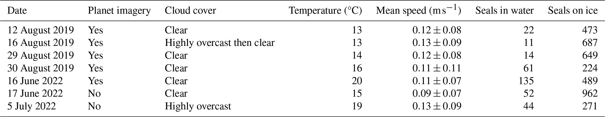
Table 1 Data availability, cloud cover, air temperature, daily average fjord speed, and number of seals in the water and on ice for the relevant aerial photographic surveys in June, July, and August of 2019 and 2022. Cloud cover and air temperature were recorded during aerial surveys.

To help interpret the variability in iceberg habitat that we observed, we also analyzed temperature and precipitation data at Lone Island and Queen Inlet (Fig. 1), which are 47 and 25 km away from Johns Hopkins Inlet, respectively, and are at elevations of 26 m and 319 $\mathrm{m}\mathrm{a}.\mathrm{s}.\mathrm{l}.$ (above sea level). Both sites consist of Campbell Scientific research-grade weather stations and are part of a long-term monitoring network to record weather and climate conditions in Glacier Bay and other coastal parks in Southeast Alaska (Bower et al., 2017). Temperature was measured within a naturally aspirated radiation shield (sensor tolerance of 0.2 °C) every 60 s and was averaged hourly; precipitation was measured continuously with a tipping bucket (resolution of 0.0254 cm) and was logged hourly. Due to instrument malfunction, we do not use the precipitation data from Lone Island, and, although the stations also recorded other meteorological parameters, such as wind speed and direction, we exclude these from our analysis due to the effects of local topography on winds.

3 Results

The iceberg-tracking algorithm produced spatially complete daily averaged velocity fields (Fig. 3) during approximately 80 % of the study period, which spanned from 20 July to 17 September 2019 and from 15 June to 26 August 2022. Large eddies commonly formed in the fjord and frequently formed at the three locations labeled I, II, and III in the streamline plots of Fig. 3. Eddy III was only observed during 2022. The eddies are also apparent in the time series of transverse velocity profiles of the fjord (Fig. 4). Periods with strong eddies appear as vertical slices containing deep-red and deep-blue colors. In the inner fjord, near the terminus of the glacier, the region of return flow shifted back and forth across the fjord, especially during 2022. In contrast, eddy II was present in the outer fjord on most days. Large eddies were also occasionally observed in the middle of the fjord (Fig. 3c and e and middle panel of Fig. 4).

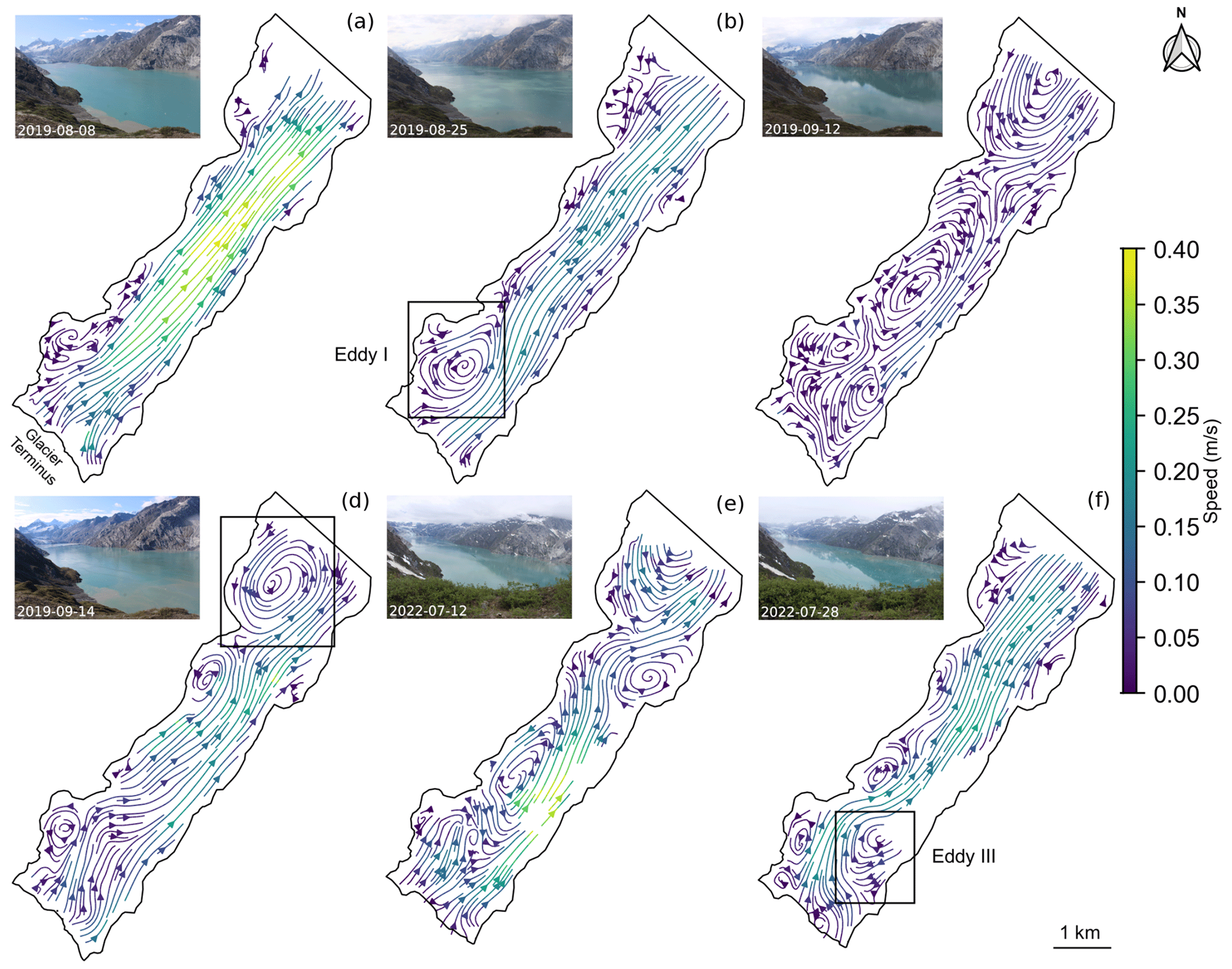
Figure 3 Streamlines derived from daily average velocity fields for select days that best characterized the range of velocity fields throughout the 2019 and 2022 field seasons. Inset photos taken from camera 3 show fjord conditions for each day. Prominent daily eddy formations that were frequently found throughout the time series are indicated in (b), (d), and (f). All maps are in WGS84 UTM Zone 8N (EPSG:32608).

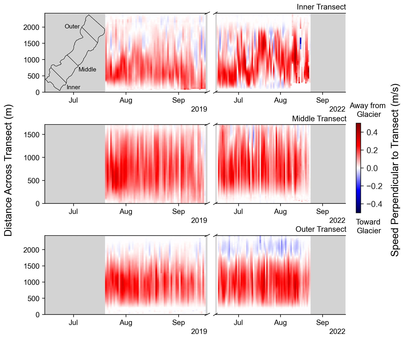
Figure 4 Time series of daily average speeds across inner, middle, and outer transects for the 2019 and 2022 field seasons. Each column represents the velocity perpendicular to the given transect on a specific date, with red colors indicating flow away from the glacier and blue colors indicating return flow toward the glacier. The inset map shows transect locations within the fjord. The distance across each transect is measured from the eastern side of the fjord.

On daily timescales, velocity fields typically experienced diurnal variations (Figs. 5 and 6). During morning hours between 05:00–13:00 (UTC-8), when runoff and katabatic (down-glacier) winds were likely to be weak, iceberg velocities were also weak and variable. The velocities typically became stronger and more uniform between 13:00–21:00 (UTC-8) as the air temperature rose and as runoff and winds increased. Tides did not appear to be a primary driver of flow variability at the fjord surface (Fig. 5).

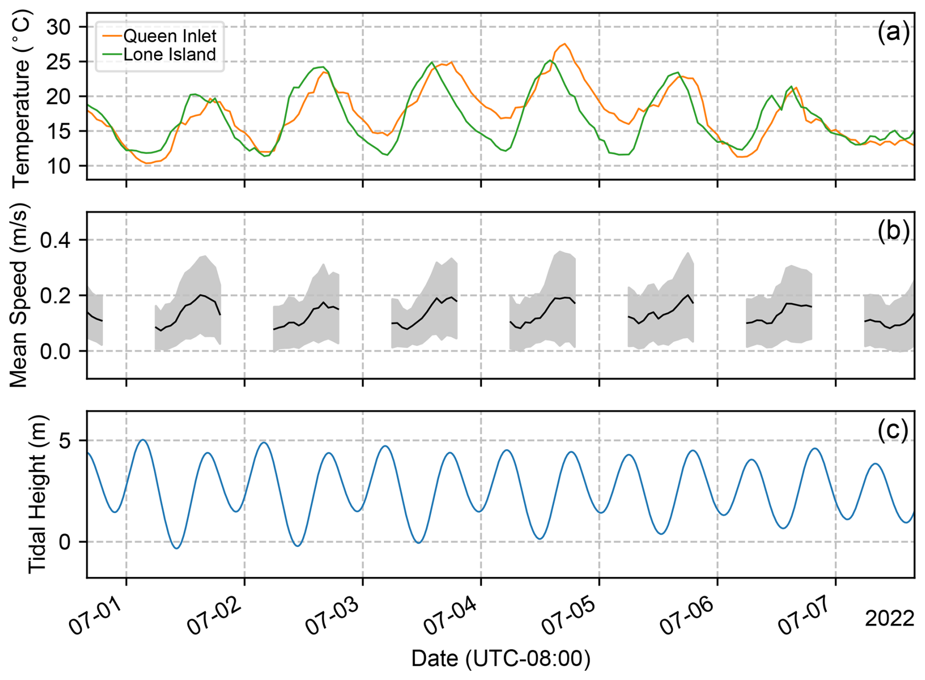
Figure 5 (a) Air temperature recorded at the Queen Inlet and Lone Island stations. The agreement between the temperatures recorded at both weather stations indicates that they are sufficient for quantifying synoptic-scale climate variability within Glacier Bay. (b) Mean and standard deviation of the flow speed within the fjord. (c) Predicted tide elevation for the Tarr Inlet tidal station.

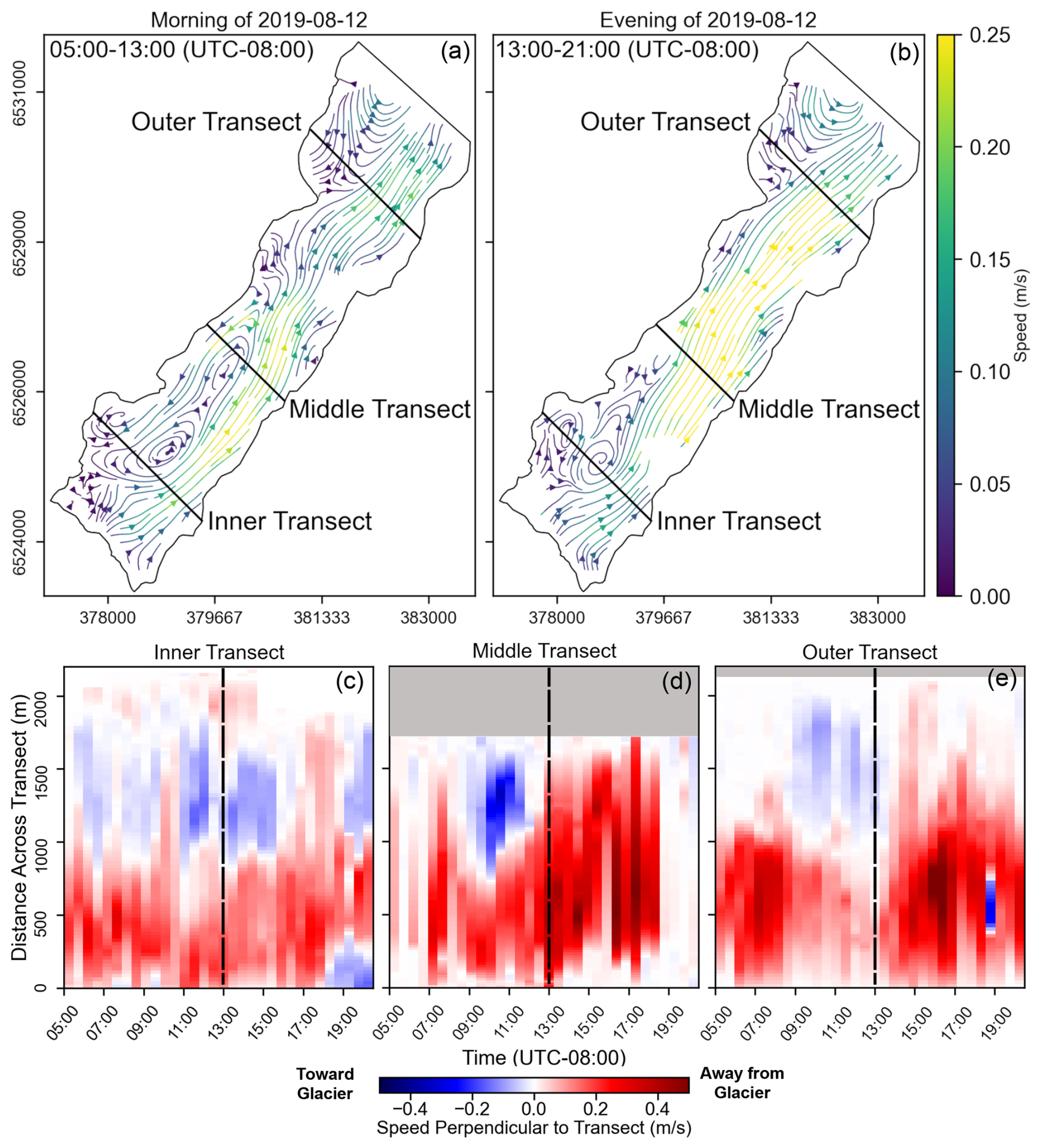
Figure 6 (a, b) Streamlines derived from velocity fields averaged over 6 h during the morning (a) and evening (b) of 12 August 2019. (c–e) Time series of hourly average speeds across the inner, middle, and outer transects for the same day. Colors represent the speed perpendicular to the transect, with red tones indicating positive (down-fjord) flow and blues indicating negative (up-fjord) flow. The distance across each transect is measured from the eastern side of the fjord.

On weekly or longer timescales, iceberg velocity patterns did not show a clear correlation with air temperature or precipitation (Fig. 7), suggesting that larger-scale circulation within Glacier Bay governs the baseline flow, upon which diurnal variations are superimposed. The fjord-averaged velocity was always in the down-fjord direction, with speeds typically ranging from 0.05 to 0.20 m s⁻¹, with a standard deviation of ∼0.1 m s⁻¹. Thus, iceberg residence times within the study area from Johns Hopkins Glacier to Jaw Point, a distance of 9 km, ranged from 0.5 to 2 d. Iceberg speed distributions were similar in June and August (average speed: 0.10 m s⁻¹) but were faster in July (average speed: 0.12 m s⁻¹).

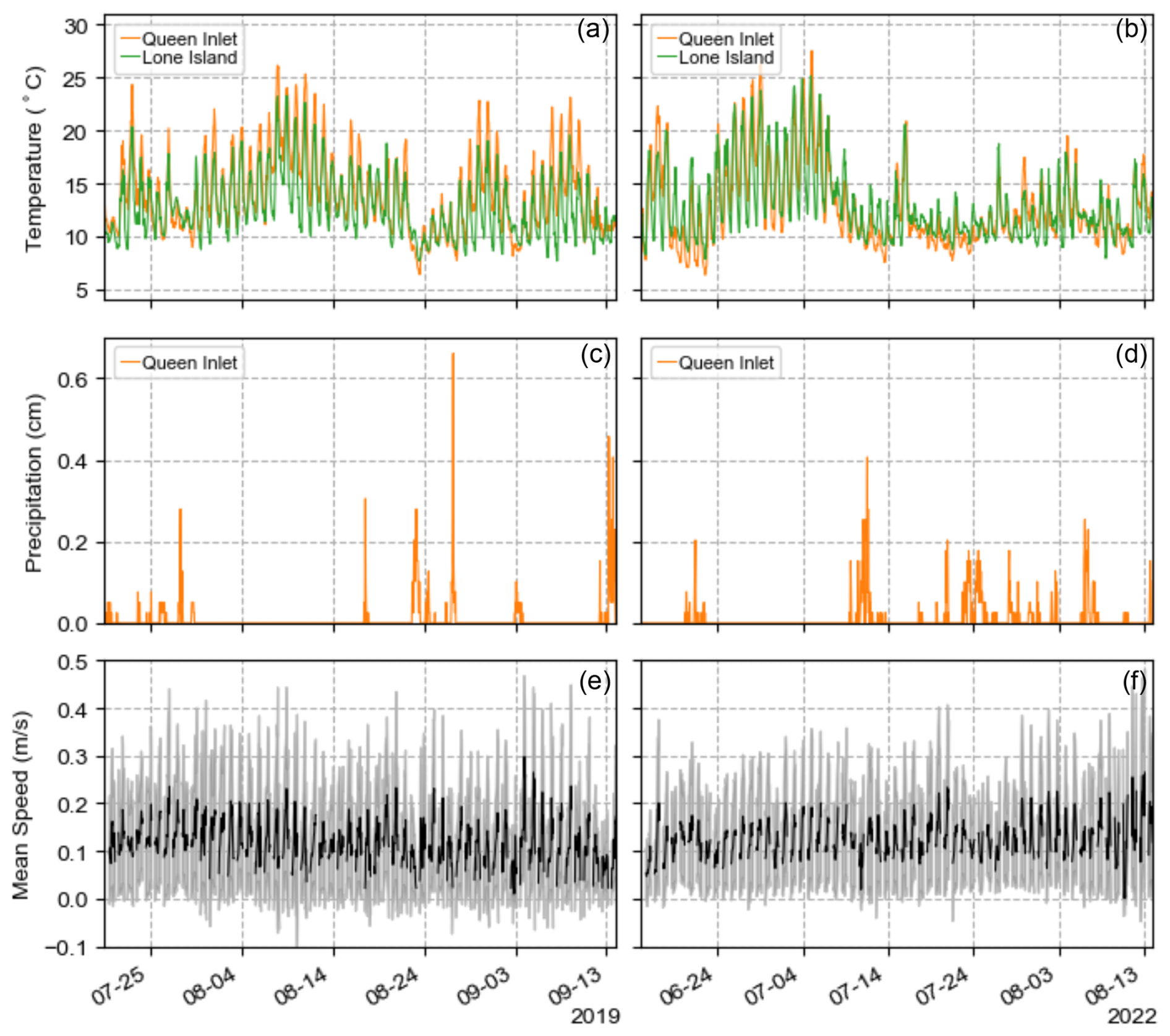
Figure 7 Meteorological data from Queen Inlet and Lone Island stations, including temperature (a, b) and precipitation (c, d) for 2019 and 2022 field seasons. (e, f) Concurrent hourly mean iceberg speed from iceberg tracking shown in black, along with standard deviation in gray.

An active glacial sediment plume was found on all aerial survey days with the available optical satellite imagery from PlanetScope (Table 1) and typically extended 4–5 km from the glacier terminus. The outflow of the plume primarily occurred on the eastern side (Fig. 8a and c) or in the central portion of the terminus (Fig. 8b). The plume location closely aligned with the velocity streamline data, with regions of faster flow within the plume extent and eddies forming along the periphery. Additionally, icebergs tended to cluster around the edges of the plume.

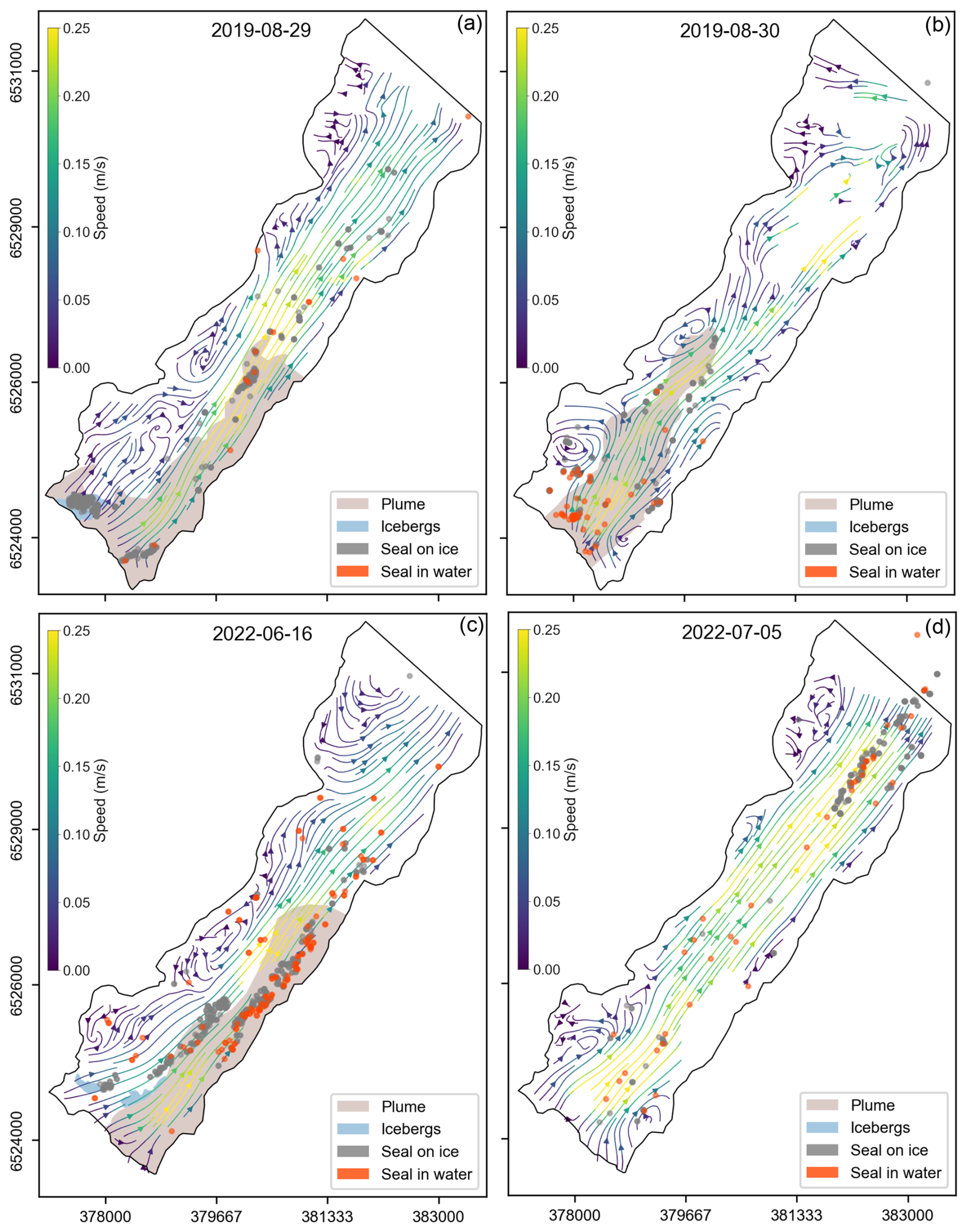
Figure 8 Streamlines derived from velocity fields averaged over 4 h periods that coincided with the timing of aerial seal surveys conducted during the molting season in 2019 (a, b) and the pupping season in 2022 (c, d). Time periods were centered on the midpoint of the aerial survey times. Seals spotted on icebergs and in surface waters are marked with gray and orange dots, respectively. Concurrent Planet satellite imagery was used to identify plume outlines and regions containing recently calved icebergs. Recently calved icebergs – defined as those near the terminus that have not yet dispersed throughout the fjord and that are likely to have calved within a few hours of the satellite image – are shown in blue, while plumes are indicated in brown. No plume data were available for 5 July 2022 due to poor satellite image quality.

Aerial photographic surveys of seals overlapped with the time-lapse photography campaign across seven dates (Table 1). During the molting period in 2019 (survey dates: 12, 16, 29, and 30 August), the majority of seals were hauled out onto icebergs in the inner portions of the fjord near the glacier terminus, where icebergs were present from recent calving events. However, on 29 August, the seals were distributed much more extensively along the length of the fjord in addition to two clusters of seals near the termini of the Johns Hopkins and Gilman glaciers. In contrast, during the pupping period in 2022 (survey dates: 16 and 17 June), seals were more uniformly distributed along the fjord and less clustered near the glacier terminus. On 5 July, the majority of the seals were found on icebergs in the outer portion of the fjord near Jaw Point and corresponded to increased iceberg speed. Occasionally, seals were observed in the water, traveling or floating at the surface, and were not hauled out onto icebergs. However, due to glacial silt in water, only seals that were in the upper meter of the water column were able to be detected during surveys.

We observed several patterns when linking seal locations to fjord velocities and plume extent. First, the seals were often located on icebergs within or along the edge of the plume and close to the glacier terminus (Fig. 8a–c), near regions of recently calved icebergs. When seals were observed in the water, they were predominantly found within the plume region. Second, when iceberg velocities were high (e.g., Fig. 8d), such as on 5 July, the seals were increasingly likely to be found in the outer part of the fjord, closer to Jaw Point, several kilometers from the glacier terminus. Finally, in the molting season, seals were more likely to be found on relatively fast-moving icebergs than during the pupping season.

The higher likelihood of finding seals on fast-moving icebergs can be seen by comparing the CCDFs of the fjord and seal velocities (Fig. 9). For both the 2019 molting and 2022 pupping seasons, about 20 % of the fjord surface was flowing faster than 0.22 m s⁻¹. Differences in the CCDFs of the seal velocities from 2019 to 2022 are largely attributable to differences in fjord circulation patterns during these two time periods. However, the CCDFs of the seal velocities do not exactly match those of the fjord velocities. When the CCDFs of the seal velocities lie above the respective curves for the fjord velocities then there is a higher probability of randomly selecting a seal at that velocity than there is of randomly selecting a fjord cell at that same velocity. The difference between the fjord velocity and seal velocity CCDFs is most apparent during the 2019 molting season. Approximately 15 % of the observed seals were located in regions of the fjord that were moving faster than 0.32 m s⁻¹, yet only 5 % of the fjord was moving at those speeds, suggesting that, during the 2019 molting period, seals tended to use icebergs in faster-flowing regions of the fjord (i.e., near the plume). In contrast, during the 2022 pupping period, fewer than 5 % of the seals were found in regions of the fjord that were flowing faster than 0.25 m s⁻¹, which is less than predicted from the fjord velocity distribution.

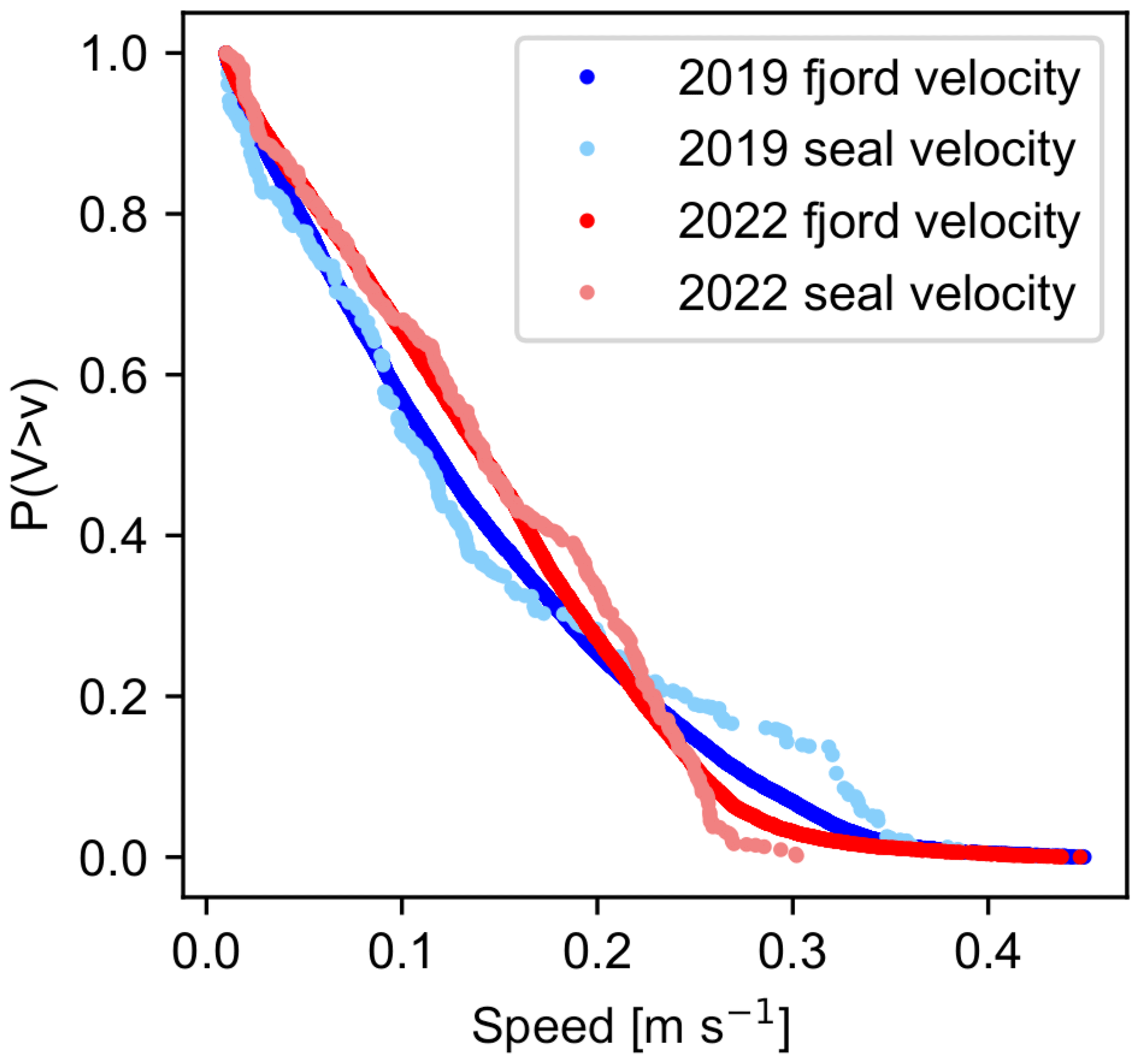
Figure 9 Complementary cumulative distribution plot for all aerial survey dates. The y axis indicates the likelihood that speed V of a randomly selected seal will have a speed that is greater than v, represented by the values along the x axis. All surveys in 2019 are from August, whereas all surveys in 2022 are from June and early July. We therefore treat 2019 data as being representative of the molting season and 2022 data as being representative of the pupping season.

4 Discussion

Freshwater runoff from tidewater glaciers emerges at depth; mixes with warm, salty water; and creates buoyant plumes that rise along glacier termini (Straneo and Cendese, 2015; Truffer and Motyka, 2016). Once a plume reaches neutral buoyancy, which typically occurs at the fjord surface in Alaska during summer (e.g., Walters et al., 1988; Bartholomaus et al., 2013; Jackson et al., 2022), it turns and flows down-fjord. The rising plumes carry nutrients and zooplankton that are utilized by seabirds, such as black-legged kittiwakes (Rissa tridactyla), and marine mammals (Lydersen et al., 2014; Stempniewicz et al., 2017; Urbanski et al., 2017; Bertrand et al., 2021). Black-legged kittiwakes from an active colony approximately 0.5 km from the terminus of Johns Hopkins Glacier are regularly observed foraging in the surface waters near the terminus after glacier-calving events. Kittiwakes use the “brown zone”, the area around the subglacial discharge that includes large amounts of suspended sediments, to forage for euphausiids, which has also been documented in numerous other fjords (Urbanski et al., 2017; Stempniewicz et al., 2017).

Our observations provide support for the idea that tidewater glacier termini are biological hotspots (Lydersen et al., 2014; Urbanski et al., 2017) and that physical processes occurring at and near glacier termini can play a role in influencing iceberg habitat and the distribution and behavior of harbor seals in the fjord. Whether hauled out on ice or swimming, seals are often found within a few hundred meters of Johns Hopkins Glacier, and their location extends throughout the fjord to Jaw Point. Depending upon the availability of iceberg habitat, seals are often either within or immediately adjacent to the outflowing plume (Fig. 8), consistent with observations of ringed seals (Pusa hispida) in Svalbard (Everett et al., 2018).

Data from our study suggest that additional factors, such as velocity fields, iceberg movement, plume proximity, and life-history constraints, may influence the selection of icebergs by seals. During the pupping season, seals were more commonly found on slow-moving icebergs, which are farther from the center of the plume, whereas, during the molting season, seals were more frequently observed on fast-flowing icebergs (>0.3 m s⁻¹). When adult females are caring for dependent pups, they may prefer slower and more stable icebergs as they spend more time hauled out during lactation. In contrast, during the molting period, adult females are no longer constrained by the presence of a dependent pup, and there is presumably less of a need to haul out onto ice that is more stable. Previous studies have also demonstrated the influence of covariates including the time of day, season, weather, and tide on the proportion of seals available to be counted (Boveng et al., 2003; Mathews and Pendleton, 2006). Collectively, the distribution and abundance of seals in tidewater glacier fjords likely reflects a complex combination of both abiotic and biotic factors.

As demonstrated by Kienholz et al. (2019), the iceberg velocity fields can be treated as estimates of fjord surface currents. The average currents that we observed (0.05–0.20 m s⁻¹) and even the maximum currents (0.4 m s⁻¹) are below the measured minimum cost of transport (MCOT) for swimming harbor seals. Davis et al. (1985) showed that the MCOT occurred in adult and juvenile harbor seals at swimming speeds between 1.0–1.4 m s⁻¹. Thus, surface currents in tidewater glacier fjords generally would not energetically impact swimming harbor seal adults. MCOT has not been measured for dependent pups, which are often observed swimming alongside their mothers, but it is unlikely that swimming against the average flow rate in Johns Hopkins Inlet would negatively impact pups.

To further illustrate these findings, we calculate the work required by an adult seal to swim against the current for the full length of the fjord (∼9 km from Jaw Point to Johns Hopkins Glacier). We approximate the drag force acting on a seal to be

$$\begin{array}{}\text{(1)}& {\displaystyle }{\displaystyle }{F}_{\mathrm{d}}={\displaystyle \frac{\mathrm{1}}{\mathrm{2}}}{C}_{\mathrm{d}}{\mathit{\rho }}_{\mathrm{w}}A{v}^{\mathrm{2}},\end{array}$$

where C_d is the drag coefficient, ρ_w is the density of water, A is the seal's frontal area, and v is the speed of the seal with respect to the water. Note that the values for C_d and A depend on how the seal area is defined, but the product of C_dA is unaffected by that definition. The work done by a seal to swim the length of fjord L is F_dΔx, where Δx is the distance that the seal swims with respect to the water, which is moving with velocity v_w:

$$\begin{array}{}\text{(2)}& {\displaystyle }{\displaystyle }\mathrm{\Delta }x=L\left({\displaystyle \frac{v}{v+v_{\mathrm{w}}}}\right).\end{array}$$

Thus, the work done is

$$\begin{array}{}\text{(3)}& {\displaystyle }{\displaystyle }W={\displaystyle \frac{\mathrm{1}}{\mathrm{2}}}{C}_{\mathrm{d}}{\mathit{\rho }}_{\mathrm{w}}A{v}^{\mathrm{2}}L\left({\displaystyle \frac{v}{v+v_{\mathrm{w}}}}\right).\end{array}$$

Williams and Kooyman (1985) investigated the hydrodynamics of harbor seals and found that C_d is around 0.1 and also reported that the cross-sectional area of harbor seals is about 0.1 m² and that typical swimming speeds range from about 1.5 to 2.0 m s⁻¹. Using these values along with $v_{\mathrm{w}}=-\mathrm{0.4}$ m s⁻¹ (the negative sign implies that a seal is swimming against the current) yields 33–55 kcal of work to overcome the drag forces acting on the seal (i.e., assuming 100 % efficiency). The total cost of transport for a harbor seal swimming at 1.5 m s⁻¹ is about 2.5 $\mathrm{J}{\mathrm{m}}^{-\mathrm{1}}{\mathrm{kg}}^{-\mathrm{1}}$ (Davis et al., 1985). Assuming a mass of 85 kg and using the distance in Eq. (2) results in a cost of transport of 200–220 kcal, which is a small fraction of the roughly 6000 kcal that seals consume every day (Härkönen and Heide-Jørgensen, 1991; Rosen and Renouf, 1998). Therefore, fjord currents likely have little direct impact on harbor seals. Currents have many indirect impacts, though, such as (i) affecting the distribution of water masses, nutrients, and small prey; (ii) contributing to the melting of glacier termini and icebergs, the former of which affects iceberg-calving rates (Ma and Bassis, 2019); and (iii) affecting the distribution of icebergs within a fjord.

5 Conclusions

High-rate time-lapse photography reveals that iceberg velocity fields in Johns Hopkins Inlet are highly variable, both temporally and spatially, during summer. During the morning hours, weak flow and large, slow-flowing eddies are generally observed. As the day progresses and temperatures and katabatic winds increase, the flow speeds increase and tend to become more uniform, with eddies becoming smaller and more icebergs being directed down-fjord towards Jaw Point. Eddy locations are variable in the inner fjord, ranging from one side of the fjord to the other, whereas eddies in the outer fjord are much more persistent. The mean velocity is always directed down-fjord and varies from 0.05 to 0.2 m s⁻¹, implying an iceberg residence time in the fjord of 0.5–2 d.

A lack of suitable climate, glaciological, and oceanographic measurements within Johns Hopkins Inlet preclude a detailed analysis of the mechanisms driving the observed flow variability. Nonetheless, our observations are consistent with a general understanding of fjord circulation that has emerged over the past 2 decades. Subglacial discharge from tidewater glaciers mixes with warm salty water at depth and drives a buoyancy-driven circulation (Straneo and Cendese, 2015; Truffer and Motyka, 2016). The strength of the buoyancy-driven circulation depends on the magnitude of the subglacial discharge (Carroll et al., 2015), which typically peaks in the afternoon on daily timescales and in middle to late summer on seasonal timescales (e.g., Jackson et al., 2022), and the location of the plume may vary seasonally as the subglacial drainage system evolves (e.g., Schild et al., 2016; Cook et al., 2020). Thus, the eddies near the terminus of Johns Hopkins Glacier appear to be controlled primarily by changes in the subglacial outlet, whereas eddies located in the outer fjord are a result of flow past topographic features. Other processes, such as winds (Straneo et al., 2010) and sill-generated mixing (Hager et al., 2022), can modify the buoyancy-driven circulation pattern so that there is not always a one-to-one correlation between subglacial discharge and fjord or iceberg velocities, especially over longer timescales. Nonetheless, subglacial discharge, through its effect on fjord circulation, appears to be an important driver of variability in iceberg habitat for seals, especially in the near-terminus region and over diurnal timescales.

Aerial photographic surveys of harbor seals that coincided with our time-lapse imagery suggest seasonal differences in the iceberg habitat used by seals. During the pupping season, the seals are rarely found on icebergs exceeding 0.2 m s⁻¹. In contrast, during the molting season, high concentrations of seals are found on icebergs exceeding 0.2 m s⁻¹. This suggests that mothers may prefer to stay in slow-flowing waters that provide safer and more stable iceberg habitats during the pupping season. However, later in summer, during the molting season, the stability of the ice habitat may be less important as pups have already been weaned and the fidelity of seals to the ice habitat is reduced. Since iceberg velocities and persistence in the fjord are linked to glacier runoff, changes in the timing and duration of the melt season or in the intensity of melt or precipitation events may influence harbor seals by reducing the availability of slow-flowing and stable icebergs during the pupping season, which may have implications for young pups that are vulnerable to predation and still dependent upon their mothers for energy. Furthermore, if ice is moving faster and is less persistent, seals may spend more time in the water swimming and repositioning to find more suitable and stable ice, which could result in increased energy expenditure, particularly for recently weaned pups that are at greater risk of a negative energy balance.

In addition to the higher likelihood of seals being found on fast-moving icebergs, we observed a strong connection between seal locations and plume extent. Seals on icebergs were often positioned within or along the edge of the plume, while seals in the water were predominantly found within the plume region. Future investigations should further explore the relationship between seal proximity to plume location to better predict where seals are likely to be found. In particular, using remote sensing techniques to spatially quantify water surface turbidity, such as the methodology presented in Hartl et al. (2025), would provide valuable insights. Additionally, expanding aerial survey efforts into July, particularly given the observed increase in surface currents during that month, could shed light on how faster glacial outflow currents influence seal distribution. Furthermore, our study was limited to aerial and time-lapse observations; incorporating oceanographic measurements in future research and focusing on a statistical analysis of seal distribution and its correlation to variables such as water temperature and salinity would provide a more comprehensive understanding of glacier runoff, ice–ocean interactions, and their implications for ice habitats.

Tidewater glacier fjords are dynamic and rapidly changing due to physical processes occurring along the ice–ocean interface that are driven by local environmental factors in combination with larger-scale climatic forcing. Collectively, these physical changes, which are rapidly occurring, will have downstream impacts and influence nutrient cycling, invertebrate and vertebrate species, food webs, and marine ecosystems in fjords (e.g., Straneo et al., 2019; Hopwood et al., 2020). Interdisciplinary studies that focus on linking the impacts of physical change to species and biological systems, coupled with long-term monitoring, will be essential to elucidating how climate change will influence tidewater glacier fjord systems.